Weight Reduction Finite Element Study of Selected Power Train Components for … · ·...
98
i Phase II Progress Report No. F/MAE/NG/-2016-02 Weight Reduction Finite Element Study of Selected Power Train Components for Heavy Duty Vehicles Submitted to FIERF and AISI By James Lowrie, Research Assistant Gracious Ngaile, Associate Professor North Carolina State University Department of Mechanical and Aerospace Engineering Advanced Metal Forming and Tribology Laboratory (AMTL) April 4, 2016 For Restricted Distribution Only (Approval must be requested from the AMTL authority prior to distribution to other organizations or individuals)
Transcript of Weight Reduction Finite Element Study of Selected Power Train Components for … · ·...

i
Phase II Progress Report No. F/MAE/NG/-2016-02
Weight Reduction Finite Element Study of Selected Power Train Components
for Heavy Duty Vehicles
Submitted to FIERF and AISI
By
James Lowrie, Research Assistant
Gracious Ngaile, Associate Professor
North Carolina State University
Department of Mechanical and Aerospace Engineering
Advanced Metal Forming and Tribology Laboratory (AMTL)
April 4, 2016
For Restricted Distribution Only
(Approval must be requested from the AMTL authority prior to distribution to other
organizations or individuals)

ii
FOREWORD This document has been prepared by the Advanced Metal Forming and Tribology Laboratory in
the Department of Mechanical and Aerospace Engineering at North Carolina State University. The
research focus of this Lab includes manufacturing process modeling and optimization, triboscience
and tribotechnology, tool design, and computational tools. In addition to conducting industry
relevant engineering research, the Lab has the objectives a) establish close cooperation between
industry and the university, b) train students, and c) transfer the research results to interested
companies.
This report, entitled “Weight Reduction Finite Element Study of Selected Power Train
Components for Heavy Duty Vehicles”, examines the potential for the reduction in the weight of
several heavy duty truck components through the finite element method. The loading conditions
on the parts are first established via a combination of surveys of individual parts and larger systems
and mathematical analysis. The several lightweight designs of some selected components are then
compared to the conventional part design to determine the potential weight savings that are
possible if the lightweight techniques were adopted.
For further information, contact Dr. Gracious Ngaile, located at North Carolina State University,
Department of Mechanical & Aerospace Engineering, 911 Oval Drive – 3160 Engineering
Building III, BOX 7910, Raleigh, NC, 27695-7910, phone: 919-515-5222,
email:[email protected], webpage:http://www.mae.ncsu.edu/ngaile.

iii
Table of Contents Chapter 1 Introduction, Motivation, and Objectives .................................................................. 1
Chapter 2 Load Map and Free Body Diagrams ......................................................................... 3
2.1 Engine Load Map ............................................................................................................. 5
2.2 Gearbox Load Map .......................................................................................................... 8
2.3 Rear Axle Load Map ...................................................................................................... 12
2.4 Summary ........................................................................................................................ 14
Chapter 3 Axle Shaft: Finite Element Study on Lightweight Shafts ....................................... 15
3.1 Introduction .................................................................................................................... 15
3.2 Solid Axle Shaft (Baseline) ............................................................................................ 16
3.3 Hollow Axle Shaft ......................................................................................................... 18
3.4 Bimetallic Axle Shaft ..................................................................................................... 24
3.5 Conclusion ..................................................................................................................... 30
Chapter 4 Input Shaft: Finite Element Study on Lightweight Shafts....................................... 31
4.1 Introduction .................................................................................................................... 31
4.2 Solid Input Shaft (Baseline) ........................................................................................... 33
4.3 Hollow Input Shaft ......................................................................................................... 35
4.4 Bimetallic Input Shaft .................................................................................................... 42
4.5 Conclusion ..................................................................................................................... 49
Chapter 5 Output Shaft: Finite Element Study on Lightweight Shafts .................................... 50
5.1 Introduction .................................................................................................................... 50
5.2 Solid Output Shaft (Baseline) ........................................................................................ 52
5.3 Hollow Output Shaft ...................................................................................................... 54
5.4 Bimetallic Output Shaft.................................................................................................. 60
5.5 Conclusion ..................................................................................................................... 67
iv
Chapter 6 Countershaft: Finite Element Study Light Weight Shafts ....................................... 68
6.1 Introduction .................................................................................................................... 68
6.2 Solid Countershaft (Baseline) ........................................................................................ 70
6.3 Hollow Countershaft ...................................................................................................... 74
6.4 Bimetallic Countershaft ................................................................................................. 80
6.5 Conclusions .................................................................................................................... 85
Chapter 7 Conclusions and Future Work ................................................................................. 87
References ............................................................................................................................ 89
v
Table of Figures
Figure 2-1: Loads acting on a Typical Tractor Trailer Configuration ........................................... 3
Figure 2-2: Loads on the Chassis and Drive Train Assembly [2].................................................. 4
Figure 2-3: Engine Load Map and Loading of Individual Engine Components ........................... 7
Figure 2-4: In Cylinder Pressure as a Function of the Crank Angle .............................................. 7
Figure 2-5: Slider Crank Mechanism ............................................................................................. 8
Figure 2-6: Gearbox Load Map and Loading of Individual Gearbox Components .................... 11
Figure 2-7: Rear Axle Load Map and Loading of Individual Gearbox Components .................. 13
Figure 3-1: Geometry and Loads on the Fully Floating Axle Shaft ............................................ 16
Figure 3-2: Geometry, Boundary Conditions, and Mesh used in the Baseline Simulations ....... 17
Figure 3-3: Stress [MPa] in the Solid Axle Shaft ........................................................................ 18
Figure 3-4: Cross Sectional View of the Stress Distribution in the Axle Shaft ............................ 18
Figure 3-5: Stress Distribution in a Hollow Shaft with an Outer Diameter of 47.6 mm [1.875 in]
and an Inner Diameter of 6.35 mm [0.25 in] .......................................................................... 19
Figure 3-6: Stress Distribution in a Hollow Shaft with an Outer Diameter of 47.6 mm [1.875] in
and an Inner Diameter of 31.75 [1.25 in] ................................................................................ 20
Figure 3-7: Stress Distribution in a Hollow Shaft with an Outer Diameter of 50.8 mm [2 in] and
an Inner Diameter of 6.78 mm [0.267 in] ............................................................................... 21
Figure 3-8: Stress Distribution in a Hollow Shaft with an Outer Diameter of 50.8 mm [2 in] and
an Inner Diameter of 33.8 mm [1.33 in] ................................................................................. 22
Figure 3-9: Maximum Stress in the Hollow Axle Shaft as a Function of Hole Aspect Ratio for
Various Diameter Shafts ......................................................................................................... 23
Figure 3-10: Mass of the Hollow Axle Shaft as a Function of Hole Aspect Ratio for Various
Diameter Shafts ....................................................................................................................... 23
Figure 3-11: Stress Distribution in a Bimetallic Shaft with an Outer Diameter of 47.6 mm [1.875
in] and an Inner Diameter of 6.35 mm [0.25 in] ..................................................................... 25
Figure 3-12: Stress Distribution in a Bimetallic Shaft with an Outer Diameter of 47.6 mm [1.875
in] and an Inner Diameter of 31.75mm [1.25 in] .................................................................... 26
Figure 3-13: Stress Distribution in a Bimetallic Shaft with an Outer Diameter of 50.8 mm [2 in]
and an Inner Diameter of 6.78 mm [0.267 in] ........................................................................ 27
vi
Figure 3-14: Stress Distribution in a Bimetallic Shaft with an Outer Diameter of 50.8 mm [2 in]
and an Inner Diameter of 33.8 mm [1.33 in] .......................................................................... 28
Figure 3-15: Maximum Stress in the Bimetallic Axle Shaft as a Function of Hole Aspect Ratio for
Various Diameter Shafts ......................................................................................................... 29
Figure 3-16: Mass of the Bimetallic Axle Shaft as a Function of Hole Aspect Ratio for Various
Diameter Shafts ....................................................................................................................... 29
Figure 4-1: Input Shaft in the Truck Gearbox .............................................................................. 32
Figure 4-2: Input Shaft Free Body Diagram ................................................................................. 32
Figure 4-3: Geometry, Boundary Conditions, and Mesh used in the Baseline Simulations ........ 33
Figure 4-4: Stress [MPa] in the Solid Input Shaft......................................................................... 34
Figure 4-5: Cross Sectional View of the Stress Distribution in the Input Shaft ........................... 35
Figure 4-6: Geometry, Boundary Conditions, and Mesh used in the Hollow Simulations .......... 35
Figure 4-7: Stress Distribution in a Hollow Shaft with an Outer Diameter of 38.1 mm [1.5 in] and
an Inner Diameter of 6.35mm [0.25 in] .................................................................................. 36
Figure 4-8: Stress Distribution in a Hollow Shaft with an Outer Diameter of 38.1 mm [1.5 in] and
an Inner Diameter of 18.3 mm [0.75 in] ................................................................................. 37
Figure 4-9: Stress Distribution in a Hollow Shaft with an Outer Diameter of 43.9 mm [1.73 in] and
an Inner Diameter of 7.37 mm [0.29 in] ................................................................................. 38
Figure 4-10: Stress Distribution in a Hollow Shaft with an Outer Diameter of 43.9 mm [1.73 in]
and an Inner Diameter of 22.1 mm [0.871 in] ........................................................................ 39
Figure 4-11: Maximum Stress in the Input Shaft as a Function of Hole Aspect Ratio for Various
Diameter Shafts ....................................................................................................................... 41
Figure 4-12: Mass of the Input Shaft as a Function of Hole Aspect Ratio for Various Diameter
Shafts....................................................................................................................................... 41
Figure 4-13: Geometry, Boundary Conditions, and Mesh used in the Bimetallic Simulations.... 42
Figure 4-14: Stress Distribution in a Bimetallic Shaft with an Outer Diameter of 38.1 mm [1.5 in]
and an Inner Diameter of 6.35mm [0.25 in] ........................................................................... 44
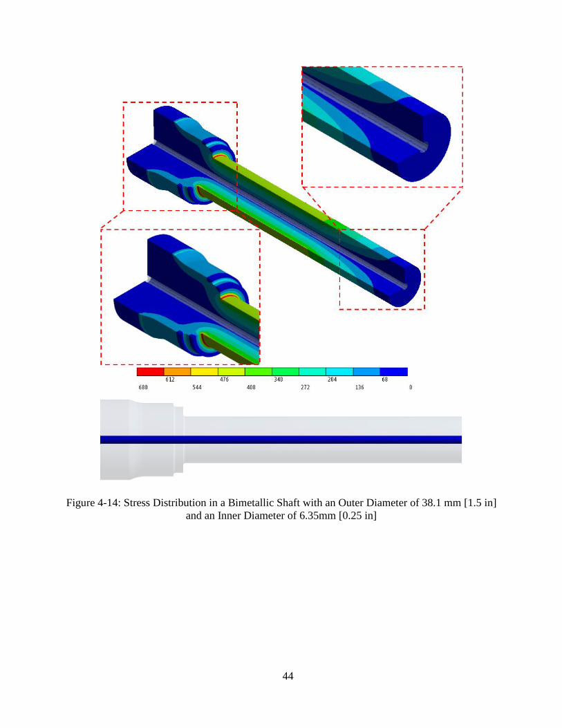
Figure 4-15: Stress Distribution in a Bimetallic Shaft with an Outer Diameter of 38.1 mm [1.5 in]
and an Inner Diameter of 18.3 mm [0.75 in] .......................................................................... 45
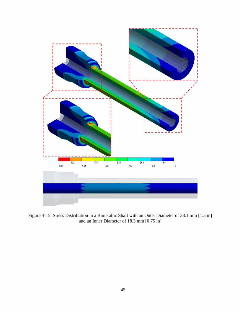
Figure 4-16: Stress Distribution in a Bimetallic Shaft with an Outer Diameter of 43.9 mm [1.73
in] and an Inner Diameter of 7.37 mm [0.29 in] ..................................................................... 46

vii
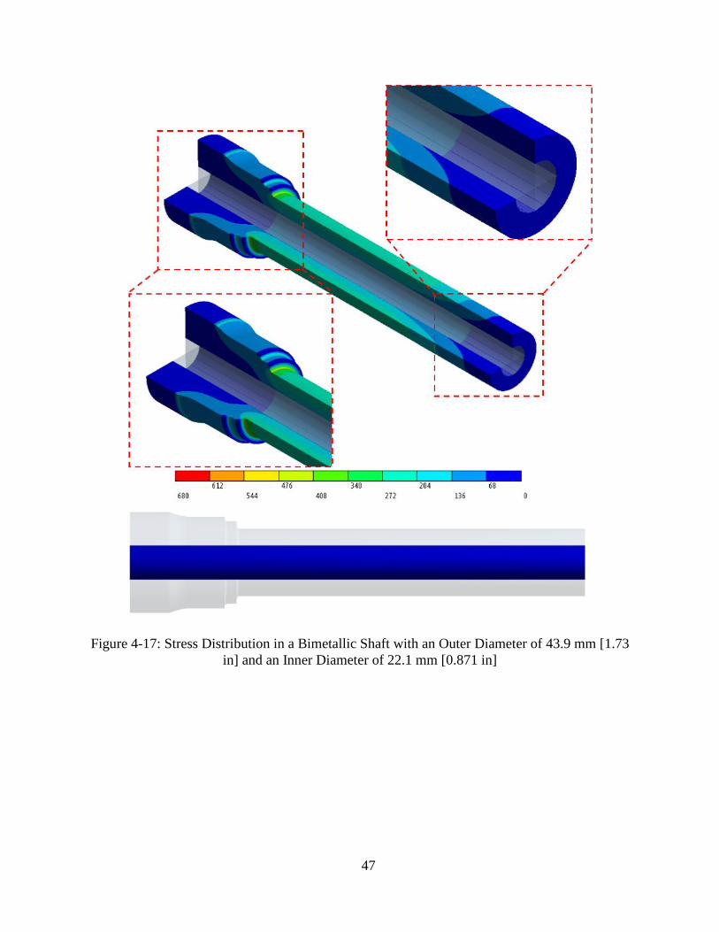
Figure 4-17: Stress Distribution in a Bimetallic Shaft with an Outer Diameter of 43.9 mm [1.73
in] and an Inner Diameter of 22.1 mm [0.871 in] ................................................................... 47
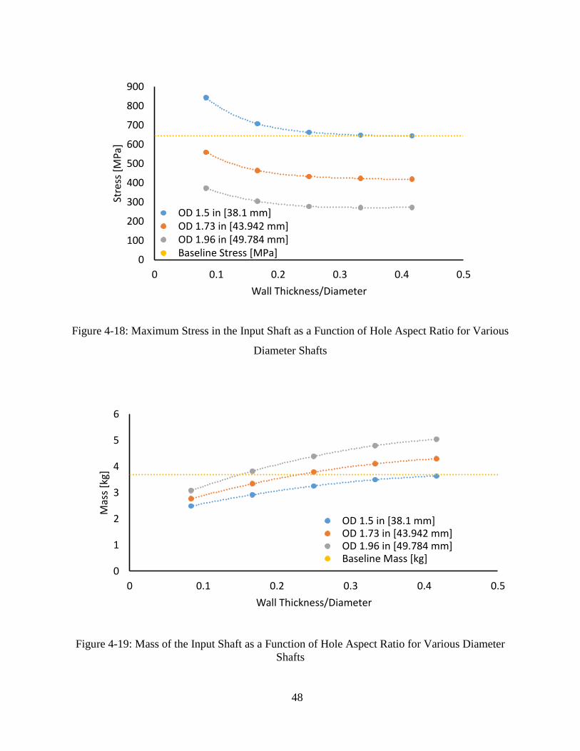
Figure 4-18: Maximum Stress in the Input Shaft as a Function of Hole Aspect Ratio for Various
Diameter Shafts ....................................................................................................................... 48
Figure 4-19: Mass of the Input Shaft as a Function of Hole Aspect Ratio for Various Diameter
Shafts....................................................................................................................................... 48
Figure 5-1: The output shaft in the truck engine........................................................................... 51
Figure 5-2: Output shaft FBD ....................................................................................................... 51
Figure 5-3: Geometry, Boundary Conditions, and Mesh used in the Baseline Simulations of the
Output Shaft ............................................................................................................................ 53
Figure 5-4: Stress [MPa] in the Solid Output Shaft ...................................................................... 54
Figure 5-5: Geometry, Boundary Conditions, and Mesh used in the Simulations of the Hollow
Output Shaft ............................................................................................................................ 55
Figure 5-6: Stress Distribution in a Hollow Output Shaft with an Outer Diameter of 49.78mm [1.96
in] and an Inner Diameter of 6.35mm [0.25 in] ...................................................................... 56
Figure 5-7: Stress Distribution in a Hollow Output Shaft with an Outer Diameter of 49.78mm [1.96
in] and an Inner Diameter of 25.4mm [1 in] .......................................................................... 57
Figure 5-8: Stress Distribution in a Hollow Output Shaft with an Outer Diameter of 57.15mm [2.25
in] and an Inner Diameter of 7.14mm [0.281 in] .................................................................... 58
Figure 5-9: Stress Distribution in a Hollow Output Shaft with an Outer Diameter of 57.15mm [2.25
in] and an Inner Diameter of 28.58mm [1.125 in] .................................................................. 58
Figure 5-10: Maximum Stress in the Hollow Output Shaft as a Function of Hole Aspect Ratio for
Various Diameter Shafts ......................................................................................................... 60
Figure 5-11: Mass of the Hollow Output Shaft as a Function of Hole Aspect Ratio for Various
Diameter Shafts ....................................................................................................................... 60
Figure 5-12: Geometry, Boundary Conditions, and Mesh used in the Simulations of the Bimetallic
Output Shaft. ........................................................................................................................... 62
Figure 5-13: Stress Distribution in a Bimetallic Output Shaft with an Outer Diameter of 49.78mm
[1.96 in] and an Inner Diameter of 6.35mm [0.25 in] ............................................................. 62
Figure 5-14: Stress Distribution in a Bimetallic Output Shaft with an Outer Diameter of 49.78mm
[1.96 in] and an Inner Diameter of 25.4mm [1 in] .................................................................. 63

viii
Figure 5-15: Stress Distribution in a Bimetallic Output Shaft with an Outer Diameter of 57.15mm
[2.25 in] and an Inner Diameter of 7.14mm [0.281 in] ........................................................... 64
Figure 5-16: Stress Distribution in a Bimetallic Output Shaft with an Outer Diameter of 57.15mm
[2.25 in] and an Inner Diameter of 28.58mm [1.125 in] ......................................................... 65
Figure 5-17: Maximum Stress in the Bimetallic Output Shaft as a Function of Hole Aspect Ratio
for Various Diameter Shafts ................................................................................................... 66
Figure 5-18: Mass of the Bimetallic Output Shaft as a Function of Hole Aspect Ratio for Various
Diameter Shafts ....................................................................................................................... 67
Figure 6-1: Mack 10 Speed Maxitorque ES T310 Gearbox with Simplified Boundary Conditions
used in Finite Element Analysis ............................................................................................. 70
Figure 6-2: Geometry and Loading on the Countershaft ............................................................. 71
Figure 6-3: (left) Countershaft with Gears, Spacers, and Key Simulated in the Baseline Finite
Element Analysis (right) Boundary Conditions applied to the Countershaft Assembly ....... 72
Figure 6-4: Mesh used in the Finite Element Simulation of the Solid Countershaft ................... 72
Figure 6-5: Stress Distribution on the Solid Countershaft (baseline) .......................................... 74
Figure 6-6: Representative Mesh used in the Finite Element Study of the Hollow Countershaft 75
Figure 6-7: Stress Distribution in a Hollow Countershaft with and Outer Diameter of 44.1mm
[1.735 in] and an internal Diameter of 6.35 mm [0.25 in] ...................................................... 76
Figure 6-8: Stress Distribution in a Hollow Countershaft with and Outer Diameter of 44.1mm
[1.735 in] and an internal Diameter of 25.4 mm [1 in] ........................................................... 77
Figure 6-9: Stress Distribution in a Hollow Countershaft with and Outer Diameter of 50.8 mm [2
in] and an internal Diameter of 7.32 mm [0.288 in] ............................................................... 78
Figure 6-10: Stress Distribution in a Hollow Countershaft with and Outer Diameter of 50.8 mm
[2 in] and an internal Diameter of 29.3 mm [1.153 in] ........................................................... 78
Figure 6-11: Maximum Stress in the Countershaft as a Function of the Wall Thickness to Outer
Diameter Ratio ........................................................................................................................ 79
Figure 6-12: Stress on Opposite Side of Keyway in the Hollow Countershaft as a Function of the
Wall Thickness to Outer Diameter Ratio ................................................................................ 80
Figure 6-13: Mass of the Countershaft as Function of Wall Thickness to Outer Diameter Ratio80
Figure 6-14: Mesh used in the Finite Element Simulation of the Bimetallic Countershaft ......... 81
ix
Figure 6-15: Stress Distribution in a Bimetallic Countershaft with and Outer Diameter of 44.1mm
[1.735 in] and an internal Diameter of 6.35 mm [0.25 in] ...................................................... 82
Figure 6-16: Stress Distribution in a Bimetallic Countershaft with and Outer Diameter of 44.1mm
[1.735 in] and an internal Diameter of 25.4 mm [1 in] ........................................................... 82
Figure 6-17: Stress Distribution in a Bimetallic Countershaft with and Outer Diameter of 50.8 mm
[2 in] and an internal Diameter of 7.32 mm [0.288 in] ........................................................... 83
Figure 6-18: Stress Distribution in a Bimetallic Countershaft with and Outer Diameter of 50.8 mm
[2 in] and an internal Diameter of 29.3 mm [1.153 in] ........................................................... 83
Figure 6-19: Maximum Stress in the Bimetallic Countershaft as a Function of the Wall Thickness
to Outer Diameter Ratio .......................................................................................................... 84
Figure 6-20: Stress on Opposite Side of Keyway in the Bimetallic Countershaft as a Function of
the Wall Thickness to Outer Diameter Ratio .......................................................................... 85
Figure 6-21: Mass of the Bimetallic Countershaft as Function of Wall Thickness to Outer
Diameter Ratio ........................................................................................................................ 85
1
Chapter 1
Introduction, Motivation, and Objectives
The main focus of the project is to reduce the weight of the components which make up class 7
and 8 trucks using innovative forging techniques, improved heat treatment techniques, material
substitution, and geometric changes. In order to determine which parts have the highest potential
for weight savings and to determine the potential lightweight techniques which should be
employed to achieve these weight reductions one must have a clear understanding of the geometry
of and loading on various truck parts. Therefore this report is focused on the numerical modeling
of several heavy duty truck components and the results of weight reduction studies carried out
using these models.
The study will focus on various shafts used to transmit torque in heavy duty trucks. Namely,
the input and output shafts, the countershaft, and the fully floating axle shaft. In the future, the
study will be extended to the other components, such as the connecting rod, crank shaft, and cam
shaft. The loads on these shafts will be determined through a combination of surveys of similar
parts and mathematical analysis of the load transfer from part to part. The numerical analysis will
be carried out using the commercial finite element software ANSYS Workbench and will disregard
dynamic loads and fatigue analysis in favor of static analysis of the maximum loading condition.
The light weight techniques which will be examined include making the shafts hollow or using a
bimetallic billet which utilizes as low density core. The main objectives of the study will be to i)
create a load map of the truck which can be used to determine the loads on the various components
for future simulation, ii) carry out a series of baseline simulations on the selected parts to determine
the stress level in a conventional part, iii) perform a series of simulations on the selected parts
which are modified to reduce their weight, and iv) determine the potential weight savings that can
be achieved by innovative lightweight fabrication techniques.
In order to accomplish these goals, the study is divided into two major parts. The first part is
dedicated to understanding the distribution and magnitude of the loads on the major heavy duty
truck systems and the components that make up these systems. In this part, the way that the loads
are transferred though the power train of the truck are mapped out and free body diagrams of the
individual components are created. The second part covers weight reduction finite element studies
2
of selected power train components. This part is divided into several chapters, each investigating
individual power train parts. Chapter 3 covers the study of the axle shaft, chapter 4 covers the
study of the gearbox input shaft, Chapter 5 covers the study of the gearbox output shaft, and
Chapter 6 covers the study of the gearbox countershaft. Finally, the content of the report is
summarized in a short conclusion chapter.
3
Chapter 2
Load Map and Free Body Diagrams
The loading of each of the class 7 and 8 truck components is critical for the evaluation
lightweight alternatives to the conventional parts. This will allow the performance of light weight
designs to be compared to the conventional components. The loading conditions on each of the
components can be determined by systematically determining the loads which are transferred from
the larger assemblies to the smaller assemblies and finally to the individual parts. In this way,
loads on individual engine components, gearbox parts, etc. can be determined from information
about the loads on the truck itself. The load maps presented in this chapter are based on a five axle
tractor trailer style truck with an engine capable of producing 2440 N m [1800 lb ft], a gearbox
with 10 speeds and rated at 2400 N m [1800 lb ft], and a tandem rear axle rated at 3550 N m [2600
lb ft].
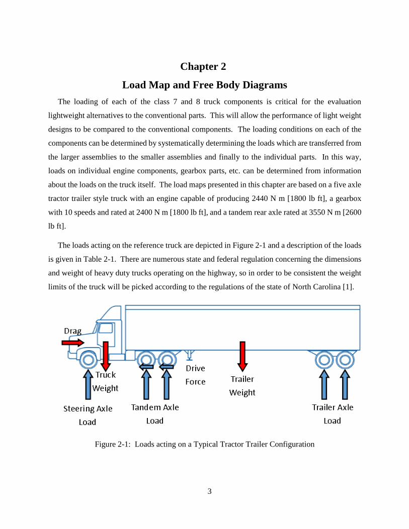
The loads acting on the reference truck are depicted in Figure 2-1 and a description of the loads
is given in Table 2-1. There are numerous state and federal regulation concerning the dimensions
and weight of heavy duty trucks operating on the highway, so in order to be consistent the weight
limits of the truck will be picked according to the regulations of the state of North Carolina [1].
Figure 2-1: Loads acting on a Typical Tractor Trailer Configuration

4
Table 2-1: Loads Acting on the Reference Vehicle
Steering Axle Load MAX 89,000 N [20,000 lbs]
Tandem Axle Load MAX 169,000 N [38,000 lbs]
Trailer Axle Load MAX 169,000 N [38,000 lbs]
Truck Weight Variable, Gross Vehicle Weight = 356 kN [80,000lbs]
Trailer Weight Variable, Gross Vehicle Weight = 356 kN [80,000lbs]
Drive Force 38,000 – 15,000 N [3,370 – 8,540 lbs]
Drag Dependent of Velocity and Wind Conditions
The focus of this investigation is to reduce the weight of the components in the heavy duty
truck, but this will not necessarily reduce the gross weight of the vehicle because as the weight of
the truck increases the weight of the cargo will be increased to maximize profits, in accordance to
state and federal weight regulations. Therefore, this study will mainly focus on components which
contribute to the weight of the unloaded truck with a special focus on the parts which can be
lightened using forging practices. By detaching the trailer and the cab to focus on these
components, a simplified free body diagram is created as shown in Figure 2-2.
Figure 2-2: Loads on the Chassis and Drive Train Assembly [2]

5
2.1 Engine Load Map
The engine is a complicated system with a high number of parts moving rapidly and with precise
timing. Based on a survey of major engine suppliers, the engines typically used in class 7 and 8
trucks are in an inline 6 configuration and have displacements of 11 to 16 L [670 to 980 in3]. They
can produce a maximum torque of anywhere from 1690 – 2780 N m [1250 – 2050 lb ft] and a
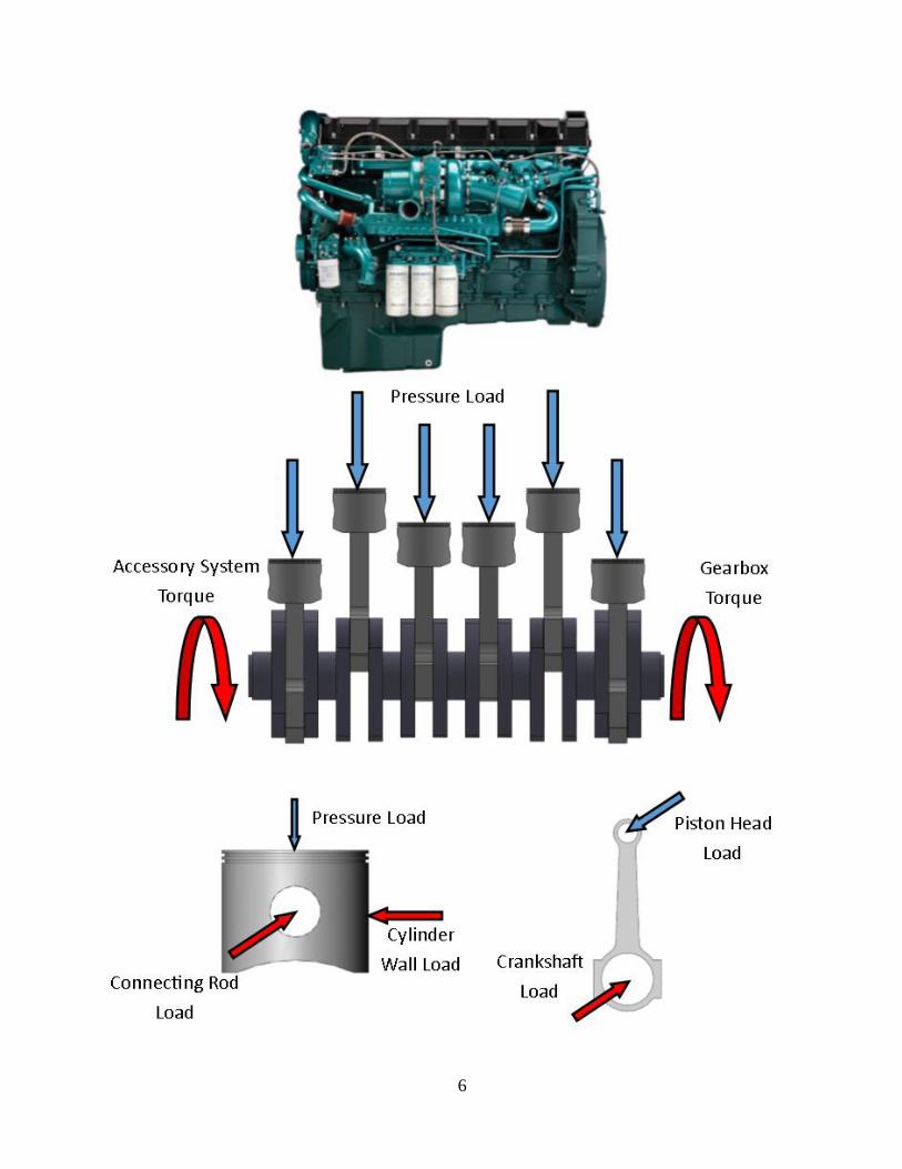
maximum power output of between 240 and 450 kW [325 and 600 HP] [3]- [5]. The parts
associated with power generation in the engine are the piston head, connecting rod, and the
crankshaft. The piston head creates a moving seal on the cylinder walls and transfers the force of
the expanding gasses from the combustion chamber to the connecting rod, which, in turn, transfers
the load onto the eccentric lobes of the crankshaft creating a torque. The majority of the torque is
then transferred to the gearbox, with the remaining torque being diverted to running the cam shafts
or auxiliary systems (e.g. air conditioning). The load transfer between the various engine
components is depicted in Figure 2-3 and information about the individual loads is given in Table
2-2.
The pressure load on the piston head depends on several parameters including the types of fuel
being used, compression ratio, type of aspiration, etc. and varies as a function of the angle of the
crank shaft. Large diesel engines are typically in a 4 stroke configuration meaning that loading on
the engine repeats itself every 720°. A typical pressure vs. crank angle plot is shown in Figure 2-4
[6]. Each of the cylinders is offset by a certain number of degrees on the crank angle to establish
the most even loading possible on the crankshaft, meaning that, in general, the pressures in the
various cylinders are not equal. Because the system is reciprocating rapidly, there are dynamic
loads which must be accounted for when determining the loads on the crank journals and piston
pins. A simplified way of accounting for the dynamics of the system is to consider the engine to
behave like a simple slider crank mechanism which is operated a constant angular velocity, as
shown in Figure 2-5.
6

7
Figure 2-3: Engine Load Map and Loading of Individual Engine Components
Table 2-2: Summary of Forces Acting on the Major Engine Components
Pressure Load MAX~15 MPa [2,175 psi] Function of Crank Angle
Gearbox Torque 2440 N – m [1800 ft – lbf]
Accessory System Torque Depends on Valve Actuating System + Other Loads from Engine
Cylinder Wall Load Function of Crank Angle and Engine Dynamics
Connecting Rod Load Function of Crank Angle and Engine Dynamics
Piston Head Load Equal and opposite to Connecting Rod Load
Crankshaft Load Function of Crank Angle and Engine Dynamics
Crankshaft Journal Loads Equal and Opposite to Individual Crankshaft Loads
Figure 2-4: In Cylinder Pressure as a Function of the Crank Angle

8
Figure 2-5: Slider Crank Mechanism
2.2 Gearbox Load Map
The gearbox is an intricate system designed to transmit an appropriate torque to the drive shaft
while keeping the engine speed in the optimal range. The gearboxes of modern day heavy duty
trucks can have as many as 15 forward speeds and 3 reverse speeds. This large number of gear
ratios is accomplished by combining 5 individual gear ratios with 3 range selectors. A simpler
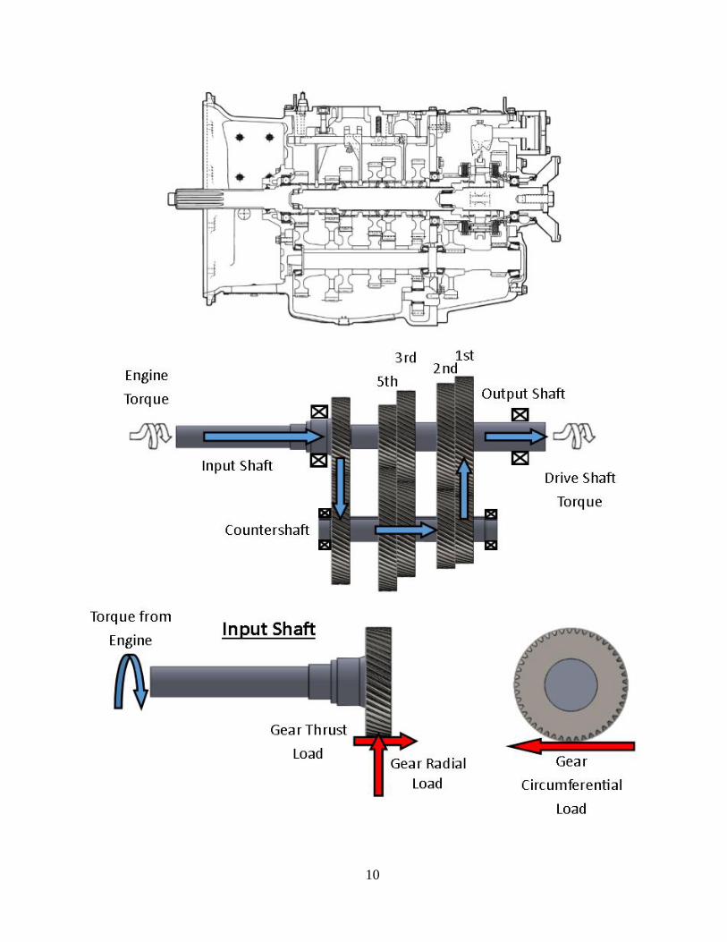
example of a gearbox with a range selection is shown in Figure 2-6 [7]. The gearbox depicted is
a 10 speed Mack T310 gearbox [8]. The torque from the engine is transmitted to the input shaft
through the splines and then transferred to the countershaft through the gear on the opposite side
of the shaft. The counter shaft receives the torque from its input gear which rotates the shaft and
all the gears on the shaft at the same speed, according to the gear ratio between the input gear and
the input shaft. The output gears of the countershaft are always engaged with the corresponding
gears on the output shaft, but only one gear transmits torque from the countershaft to the output
shaft at a time. The gear which is engaged is selected by meshing a sliding clutch on the output
shaft with the desired gear which forces the gear to rotate with the shaft, the rest of the gears on
the output shaft are free to rotate at a different speed than the shaft. The output shaft will either be
directly engaged with the drive shaft, or it will be engaged with another gear set with two to 3
speeds which allows the operator to select a gear range.
In order to transfer torque from gear to gear the meshing teeth apply forces to each other. The
magnitude of these forces is dependent on the diameter of the gear and the geometry of the teeth.
Modern day gearboxes typically have helical gears, though some gearboxes still utilize spur gears,
and most gears have a pressure angle of 20°. Table 2-3 summarizes the forces which might be
found on gears with the proportions shown in Figure 2-6. It should be noted that these loads are
determined based on the assumption that there is only one countershaft in order to properly
demonstrate the forces that are created from the meshing teeth. However, the real Mack T310

9
gearbox has 3 countershaft and many other gearboxes have 2 countershafts which allows them to
reduce the loads on the gear teeth by 1
# 𝑜𝑓 𝑐𝑜𝑢𝑛𝑡𝑒𝑟𝑠ℎ𝑎𝑓𝑡𝑠 and eliminate the bending loads on the input
and output shafts through proper balancing of the radial and circumferential loads.
10

11
Figure 2-6: Gearbox Load Map and Loading of Individual Gearbox Components
Table 2-3: Summary of Forces Acting on the Major Gearbox Components
General
Engine Torque 2,440 N – m [1,800 ft – lbf]
Drive Shaft Torque (6th Gear) 6,520 N – m [4,810 ft – lbs]
Input Shaft
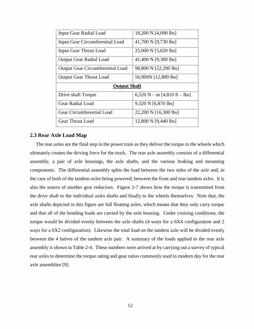
Gear Radial Load 18,200 N [4,090 lbs]
Gear Circumferential Load 41,700 N [9,730 lbs]
Gear Thrust Load 25,000 N [5,620 lbs]
Countershaft
12
Input Gear Radial Load 18,200 N [4,090 lbs]
Input Gear Circumferential Load 41,700 N [9,730 lbs]
Input Gear Thrust Load 25,000 N [5,620 lbs]
Output Gear Radial Load 41,400 N [9,300 lbs]
Output Gear Circumferential Load 98,800 N [22,200 lbs]
Output Gear Thrust Load 56,900N [12,800 lbs]
Output Shaft
Drive shaft Torque 6,520 N – m [4,810 ft – lbs]
Gear Radial Load 9,320 N [6,870 lbs]
Gear Circumferential Load 22,200 N [16,300 lbs]
Gear Thrust Load 12,800 N [9,440 lbs]
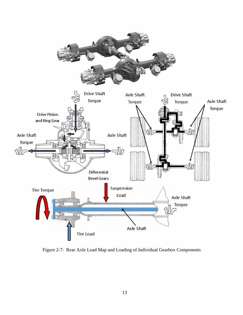
2.3 Rear Axle Load Map
The rear axles are the final step in the power train as they deliver the torque to the wheels which
ultimately creates the driving force for the truck. The rear axle assembly consists of a differential
assembly, a pair of axle housings, the axle shafts, and the various braking and mounting
components. The differential assembly splits the load between the two sides of the axle and, in
the case of both of the tandem axles being powered, between the front and rear tandem axles. It is
also the source of another gear reduction. Figure 2-7 shows how the torque is transmitted from
the drive shaft to the individual axles shafts and finally to the wheels themselves. Note that, the
axle shafts depicted in this figure are full floating axles, which means that they only carry torque
and that all of the bending loads are carried by the axle housing. Under cruising conditions, the
torque would be divided evenly between the axle shafts (4 ways for a 6X4 configuration and 2
ways for a 6X2 configuration). Likewise the total load on the tandem axle will be divided evenly
between the 4 halves of the tandem axle pair. A summary of the loads applied to the rear axle
assembly is shown in Table 2-4. These numbers were arrived at by carrying out a survey of typical
rear axles to determine the torque rating and gear ratios commonly used in modern day for the rear
axle assemblies [9].
13
Figure 2-7: Rear Axle Load Map and Loading of Individual Gearbox Components

14
Table 2-4: Summary of the Loads Acting on the Rear Axle Assembly
Drive Shaft Torque 3,550 N m [2,620 lb ft]
Axle Shaft Torque 8630 to 21,900 N m [6,370 to 16,200 lb ft]
Tire Torque Equal and Opposite to Axle Shaft Torque
Suspension Load 42,300 N [9,500 lbs]
Tire Load 42,300 N [9,500 lbs]
2.4 Summary
The loads on the truck are used to determine the loads on the major systems which make up the
truck powertrain. The loads are determined through a combination surveys of engines, gearboxes,
and rear axles and calculations based on gear ratios, geometry, and dynamic analysis. Using the
loads mapped out in this chapter detailed finite element models of the components outlined in this
report were created and employed in the study of lightweight designs of selected power train
components.
15
Chapter 3
Axle Shaft: Finite Element Study on Lightweight Shafts
3.1 Introduction
Using the loads determined in chapter 2, it is possible to create a finite element model of the
axle shaft. This finite element model is first used to examine the distribution of stresses in the
conventional, solid axle shaft. These stresses are then used as a baseline to define the required
performance of a light weight design. Two methods for reducing the weight of the shaft are then
investigated and evaluated in regards to the baseline study. Finally, the chapter is concluded with
an outlook on the possible weight savings that could be achieved by adopting the lightweight
techniques investigated.
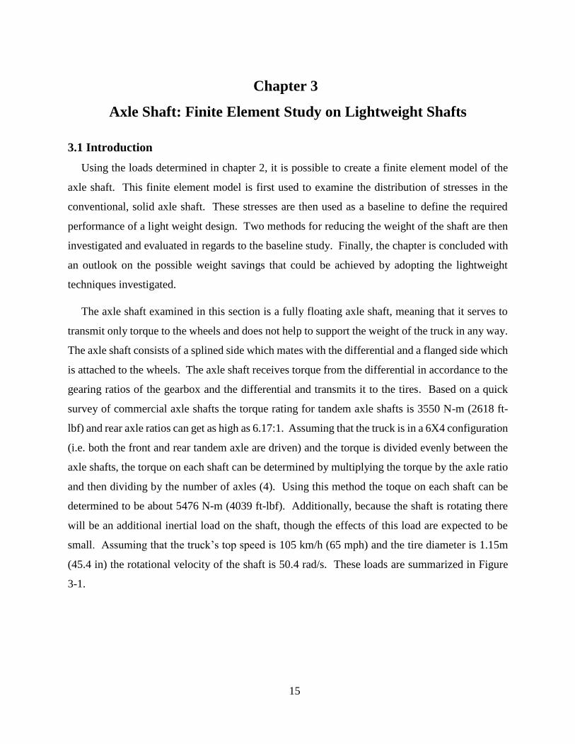
The axle shaft examined in this section is a fully floating axle shaft, meaning that it serves to
transmit only torque to the wheels and does not help to support the weight of the truck in any way.
The axle shaft consists of a splined side which mates with the differential and a flanged side which
is attached to the wheels. The axle shaft receives torque from the differential in accordance to the
gearing ratios of the gearbox and the differential and transmits it to the tires. Based on a quick
survey of commercial axle shafts the torque rating for tandem axle shafts is 3550 N-m (2618 ft-
lbf) and rear axle ratios can get as high as 6.17:1. Assuming that the truck is in a 6X4 configuration
(i.e. both the front and rear tandem axle are driven) and the torque is divided evenly between the
axle shafts, the torque on each shaft can be determined by multiplying the torque by the axle ratio
and then dividing by the number of axles (4). Using this method the toque on each shaft can be
determined to be about 5476 N-m (4039 ft-lbf). Additionally, because the shaft is rotating there
will be an additional inertial load on the shaft, though the effects of this load are expected to be
small. Assuming that the truck’s top speed is 105 km/h (65 mph) and the tire diameter is 1.15m
(45.4 in) the rotational velocity of the shaft is 50.4 rad/s. These loads are summarized in Figure
3-1.
16
Figure 3-1: Geometry and Loads on the Fully Floating Axle Shaft
3.2 Solid Axle Shaft (Baseline)
The baseline simulations of the axle shaft serve to establish the nominal stresses in a
conventional axle shaft under its maximum loading conditions. These stresses can then be
compared to the stresses observed in later simulations which utilize lightweight concepts. This
allows for the evaluations of individual light weight designs and provides some idea of the
necessary performance of the light weight component.
The geometry of the simulated axle shaft was taken from drawings of a full floating axle shaft
and the diameter of the smallest cross-section of the shaft was 47.6 mm [1.875 in]. However,
features like splines were ignored in order to simplify the simulation. It was meshed with
tetrahedral elements and the mesh was refined in areas where stress concentration were expected
(i.e. the radii) as shown in Figure 3-2. The material was approximated by ANSYS’s structural
steel model which has a Young’s Modulus of 200 GPa [29,000 ksi] and a Poisson’s ratio of 0.3.
Only the material’s elastic behaviors were simulated, as plastic deformation of the part would be
considered failure. The torque load was applied as a moment boundary condition on the area of
the shaft into which splines would be cut, and the shaft was held in place via fixed displacement
boundary conditions in the holes to which the tires are mounted on the flange. A rotational velocity
was applied to the entire shaft to simulate the inertial loads on the shaft.

17
Figure 3-2: Geometry, Boundary Conditions, and Mesh used in the Baseline Simulations
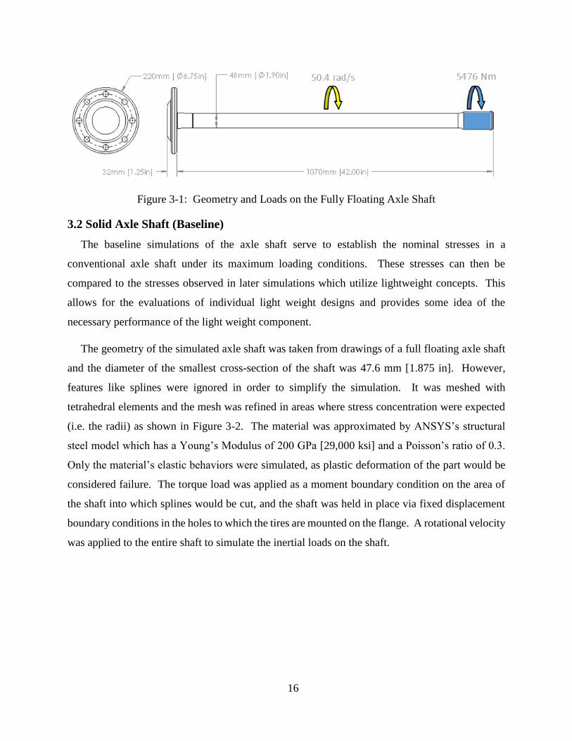
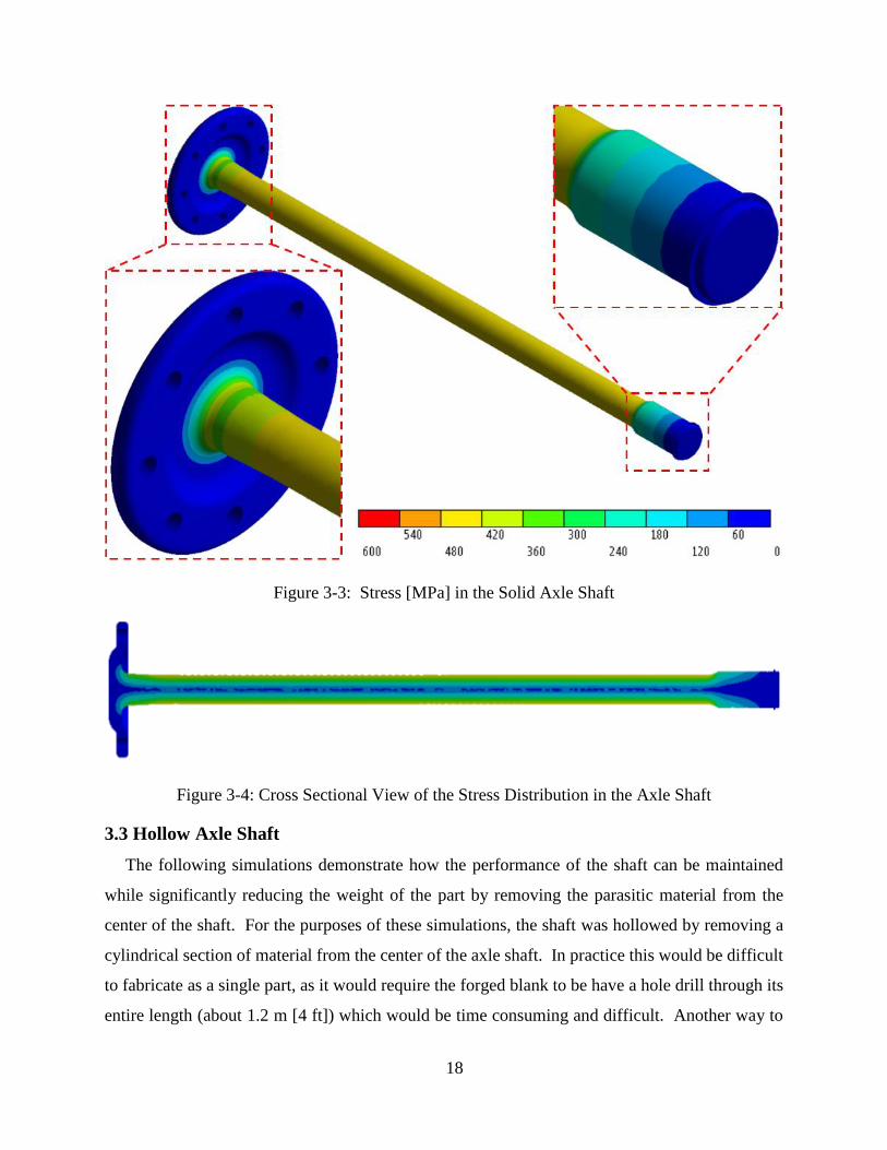
After the completion of the simulation the stress contours were plotted as shown in Figure 3-3.
The maximum stress fell into the 480 - 420 MPa [69.6 – 60.9 ksi] range and occurred in the thinnest
section of the axle shaft. Due to stress concentrations caused by the changes in diameter on the
shaft the stress was slightly higher around the transitions from the small diameter section of the
shaft to the flange and the splines. It is interesting to note that the stresses in the shaft are
concentrated on the outer diameter of the shaft and that the stress in the middle of the shaft is
almost zero, as shown in Figure 3-4. Thus the material in the middle of the shaft increases the
weight of the part without contributing significantly to its strength. The weight of the shaft could
be significantly reduced by removing this parasitic material from the inside of the shaft or by
replacing it with a lower density material.
18
Figure 3-3: Stress [MPa] in the Solid Axle Shaft
Figure 3-4: Cross Sectional View of the Stress Distribution in the Axle Shaft
3.3 Hollow Axle Shaft
The following simulations demonstrate how the performance of the shaft can be maintained
while significantly reducing the weight of the part by removing the parasitic material from the
center of the shaft. For the purposes of these simulations, the shaft was hollowed by removing a
cylindrical section of material from the center of the axle shaft. In practice this would be difficult
to fabricate as a single part, as it would require the forged blank to be have a hole drill through its
entire length (about 1.2 m [4 ft]) which would be time consuming and difficult. Another way to

19
fabricate this shaft would be to start with a thick tube and weld a flange onto its end although this
too would come at the cost of additional required equipment manufacturing steps. Perhaps the
most attractive way to fabricate this shaft would be to come up with an innovative way to forge a
flange onto a tubular blank, eliminating the need for time consuming joining and machining steps.
The first simulation which was carried out had the same outside dimensions as the baseline axle
shaft, but had a 6.35 mm [0.25 in] hole through the center of the part. The stress distribution in
this part is given in Figure 3-5. The change in the maximum stress in the part is nearly unnoticeable
with the maximum stress again falling into the 480 to 420 MPa [69.6 to 60.9 ksi] range. However,
there was also not a significant weight savings from the removal of this small amount of material
(the weight of the part was only reduced by 0.18 kg [0.4 lbs]). Clearly more material must be
removed to see significant weight savings.
Figure 3-5: Stress Distribution in a Hollow Shaft with an Outer Diameter of 47.6 mm [1.875 in]
and an Inner Diameter of 6.35 mm [0.25 in]
The effects of removing a significant amount of material were investigated in the next
simulation. Once again the outside geometry of the shaft was kept the same as the baseline
20
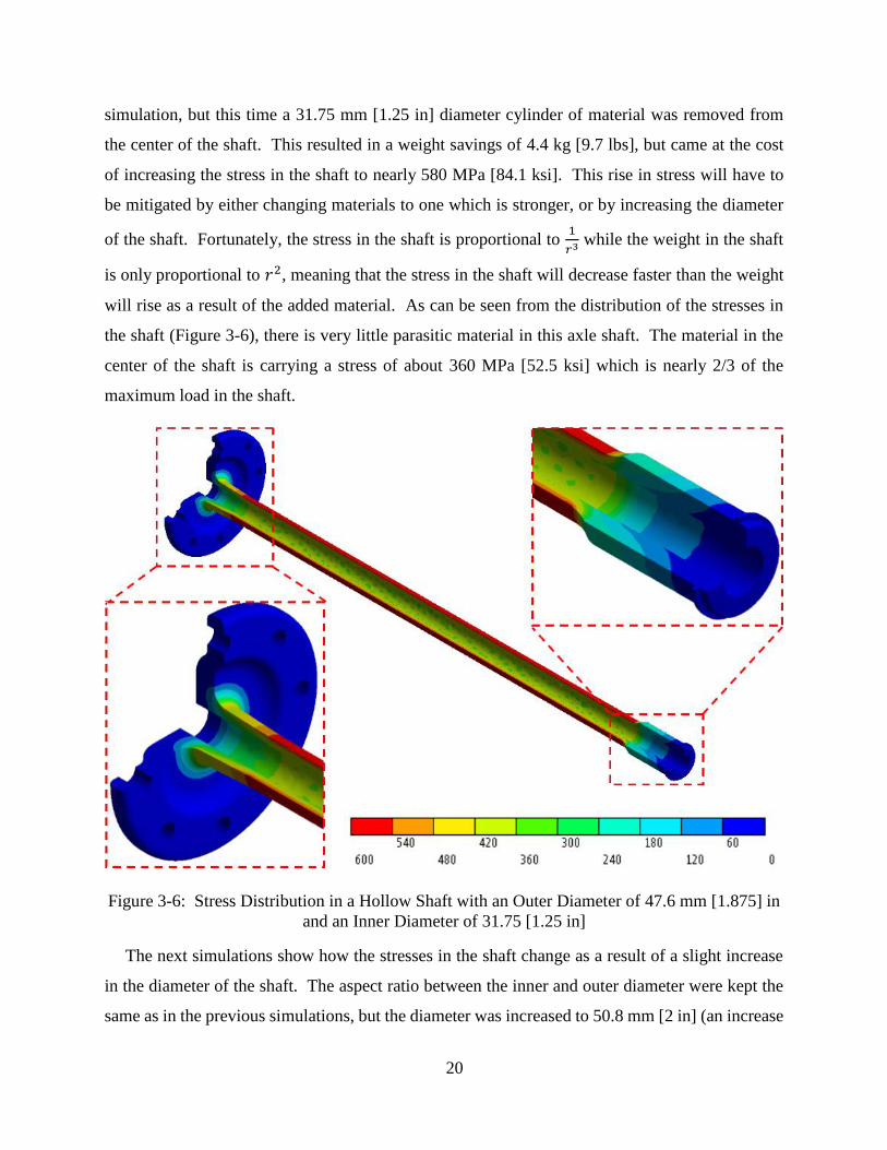
simulation, but this time a 31.75 mm [1.25 in] diameter cylinder of material was removed from
the center of the shaft. This resulted in a weight savings of 4.4 kg [9.7 lbs], but came at the cost
of increasing the stress in the shaft to nearly 580 MPa [84.1 ksi]. This rise in stress will have to
be mitigated by either changing materials to one which is stronger, or by increasing the diameter
of the shaft. Fortunately, the stress in the shaft is proportional to 1
𝑟3 while the weight in the shaft
is only proportional to 𝑟2, meaning that the stress in the shaft will decrease faster than the weight
will rise as a result of the added material. As can be seen from the distribution of the stresses in
the shaft (Figure 3-6), there is very little parasitic material in this axle shaft. The material in the
center of the shaft is carrying a stress of about 360 MPa [52.5 ksi] which is nearly 2/3 of the
maximum load in the shaft.
Figure 3-6: Stress Distribution in a Hollow Shaft with an Outer Diameter of 47.6 mm [1.875] in
and an Inner Diameter of 31.75 [1.25 in]
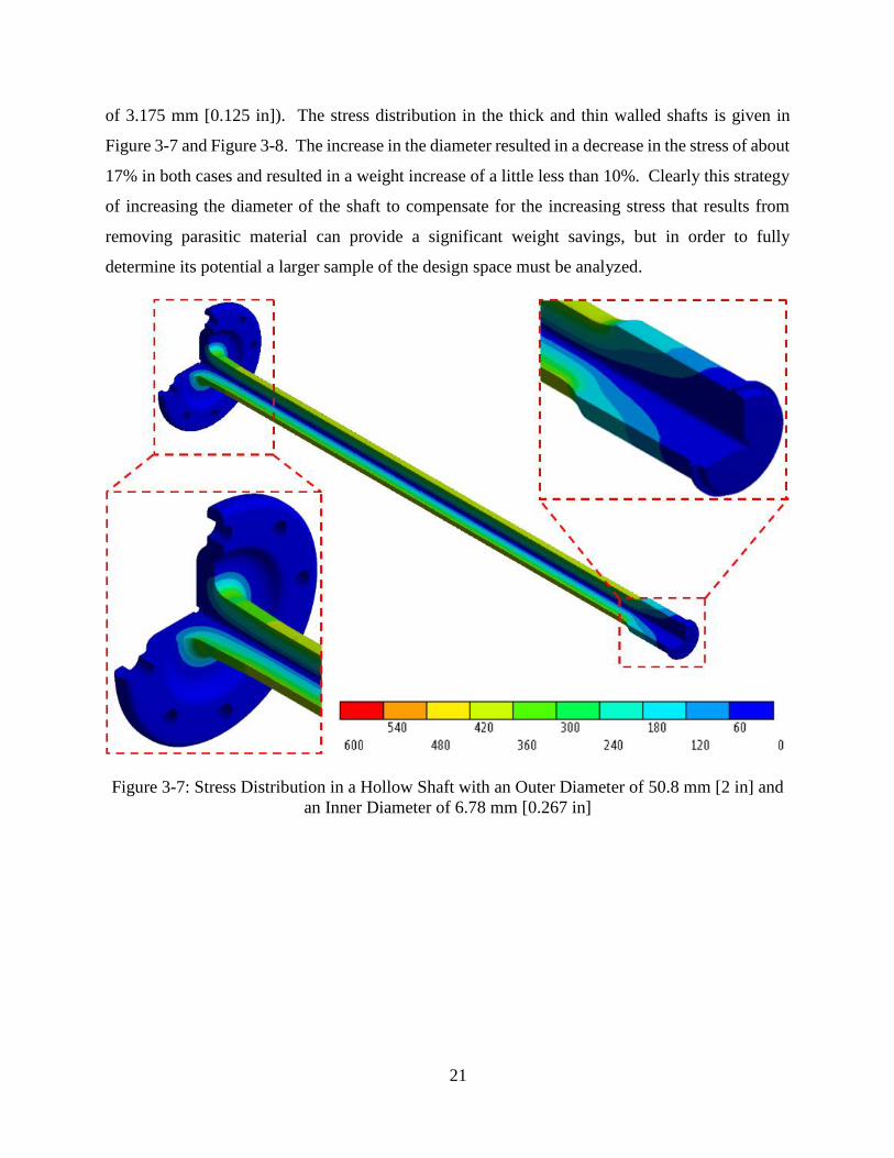
The next simulations show how the stresses in the shaft change as a result of a slight increase
in the diameter of the shaft. The aspect ratio between the inner and outer diameter were kept the
same as in the previous simulations, but the diameter was increased to 50.8 mm [2 in] (an increase
21
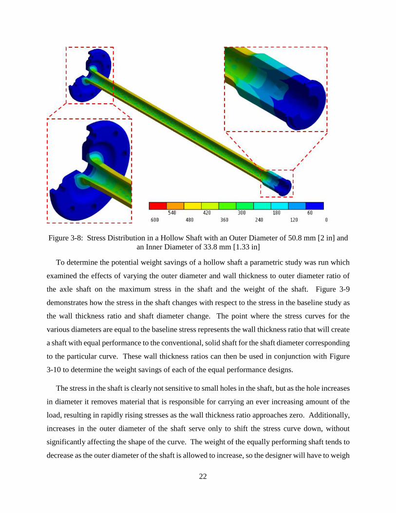
of 3.175 mm [0.125 in]). The stress distribution in the thick and thin walled shafts is given in
Figure 3-7 and Figure 3-8. The increase in the diameter resulted in a decrease in the stress of about
17% in both cases and resulted in a weight increase of a little less than 10%. Clearly this strategy
of increasing the diameter of the shaft to compensate for the increasing stress that results from
removing parasitic material can provide a significant weight savings, but in order to fully
determine its potential a larger sample of the design space must be analyzed.
Figure 3-7: Stress Distribution in a Hollow Shaft with an Outer Diameter of 50.8 mm [2 in] and
an Inner Diameter of 6.78 mm [0.267 in]
22
Figure 3-8: Stress Distribution in a Hollow Shaft with an Outer Diameter of 50.8 mm [2 in] and
an Inner Diameter of 33.8 mm [1.33 in]
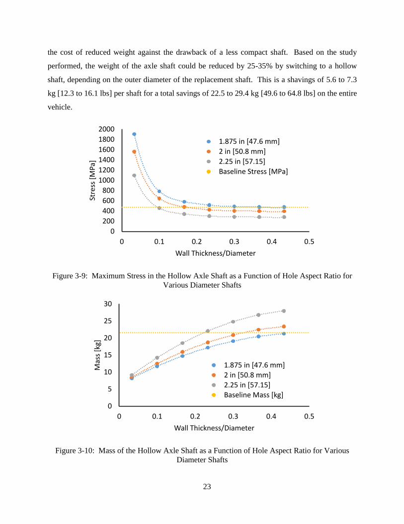
To determine the potential weight savings of a hollow shaft a parametric study was run which
examined the effects of varying the outer diameter and wall thickness to outer diameter ratio of
the axle shaft on the maximum stress in the shaft and the weight of the shaft. Figure 3-9
demonstrates how the stress in the shaft changes with respect to the stress in the baseline study as
the wall thickness ratio and shaft diameter change. The point where the stress curves for the
various diameters are equal to the baseline stress represents the wall thickness ratio that will create
a shaft with equal performance to the conventional, solid shaft for the shaft diameter corresponding
to the particular curve. These wall thickness ratios can then be used in conjunction with Figure
3-10 to determine the weight savings of each of the equal performance designs.
The stress in the shaft is clearly not sensitive to small holes in the shaft, but as the hole increases
in diameter it removes material that is responsible for carrying an ever increasing amount of the
load, resulting in rapidly rising stresses as the wall thickness ratio approaches zero. Additionally,
increases in the outer diameter of the shaft serve only to shift the stress curve down, without
significantly affecting the shape of the curve. The weight of the equally performing shaft tends to
decrease as the outer diameter of the shaft is allowed to increase, so the designer will have to weigh
23
the cost of reduced weight against the drawback of a less compact shaft. Based on the study
performed, the weight of the axle shaft could be reduced by 25-35% by switching to a hollow
shaft, depending on the outer diameter of the replacement shaft. This is a shavings of 5.6 to 7.3
kg [12.3 to 16.1 lbs] per shaft for a total savings of 22.5 to 29.4 kg [49.6 to 64.8 lbs] on the entire
vehicle.
Figure 3-9: Maximum Stress in the Hollow Axle Shaft as a Function of Hole Aspect Ratio for
Various Diameter Shafts
Figure 3-10: Mass of the Hollow Axle Shaft as a Function of Hole Aspect Ratio for Various
Diameter Shafts
0
200
400
600
800
1000
1200
1400
1600
1800
2000
0 0.1 0.2 0.3 0.4 0.5
Stre
ss [
MPa
]
Wall Thickness/Diameter
1.875 in [47.6 mm]
2 in [50.8 mm]
2.25 in [57.15]
Baseline Stress [MPa]
0
5
10
15
20
25
30
0 0.1 0.2 0.3 0.4 0.5
Mas
s [k
g]
Wall Thickness/Diameter
1.875 in [47.6 mm]
2 in [50.8 mm]
2.25 in [57.15]
Baseline Mass [kg]
24
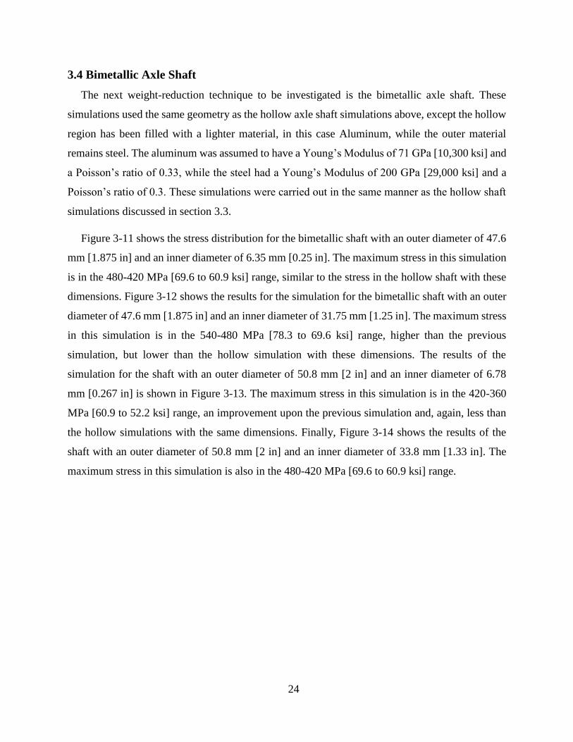
3.4 Bimetallic Axle Shaft
The next weight-reduction technique to be investigated is the bimetallic axle shaft. These
simulations used the same geometry as the hollow axle shaft simulations above, except the hollow
region has been filled with a lighter material, in this case Aluminum, while the outer material
remains steel. The aluminum was assumed to have a Young’s Modulus of 71 GPa [10,300 ksi] and
a Poisson’s ratio of 0.33, while the steel had a Young’s Modulus of 200 GPa [29,000 ksi] and a
Poisson’s ratio of 0.3. These simulations were carried out in the same manner as the hollow shaft
simulations discussed in section 3.3.
Figure 3-11 shows the stress distribution for the bimetallic shaft with an outer diameter of 47.6
mm [1.875 in] and an inner diameter of 6.35 mm [0.25 in]. The maximum stress in this simulation
is in the 480-420 MPa [69.6 to 60.9 ksi] range, similar to the stress in the hollow shaft with these
dimensions. Figure 3-12 shows the results for the simulation for the bimetallic shaft with an outer
diameter of 47.6 mm [1.875 in] and an inner diameter of 31.75 mm [1.25 in]. The maximum stress
in this simulation is in the 540-480 MPa [78.3 to 69.6 ksi] range, higher than the previous
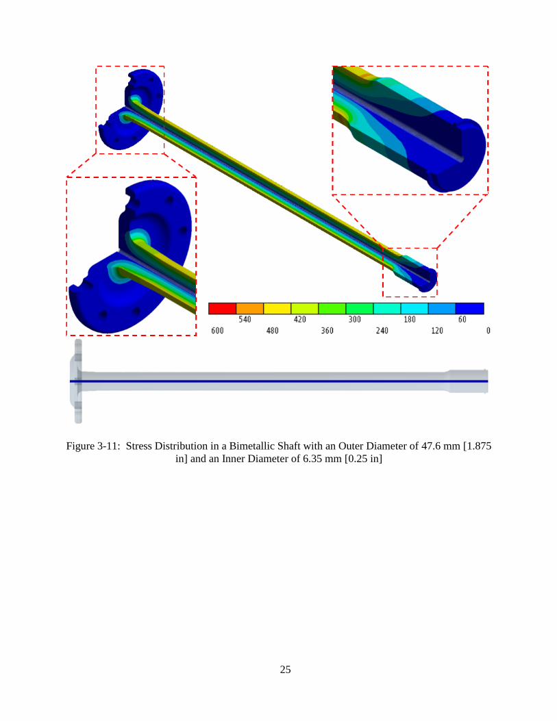
simulation, but lower than the hollow simulation with these dimensions. The results of the
simulation for the shaft with an outer diameter of 50.8 mm [2 in] and an inner diameter of 6.78
mm [0.267 in] is shown in Figure 3-13. The maximum stress in this simulation is in the 420-360
MPa [60.9 to 52.2 ksi] range, an improvement upon the previous simulation and, again, less than
the hollow simulations with the same dimensions. Finally, Figure 3-14 shows the results of the
shaft with an outer diameter of 50.8 mm [2 in] and an inner diameter of 33.8 mm [1.33 in]. The
maximum stress in this simulation is also in the 480-420 MPa [69.6 to 60.9 ksi] range.
25
Figure 3-11: Stress Distribution in a Bimetallic Shaft with an Outer Diameter of 47.6 mm [1.875
in] and an Inner Diameter of 6.35 mm [0.25 in]

26
Figure 3-12: Stress Distribution in a Bimetallic Shaft with an Outer Diameter of 47.6 mm [1.875
in] and an Inner Diameter of 31.75mm [1.25 in]
27
Figure 3-13: Stress Distribution in a Bimetallic Shaft with an Outer Diameter of 50.8 mm [2 in]
and an Inner Diameter of 6.78 mm [0.267 in]

28
Figure 3-14: Stress Distribution in a Bimetallic Shaft with an Outer Diameter of 50.8 mm [2 in]
and an Inner Diameter of 33.8 mm [1.33 in]
Another parametric study was performed on the bimetallic axle shafts in a similar manner as
the study performed on the hollow shafts. Figure 3-15 below shows the maximum stress in the
bimetallic axle shaft as a function of the aspect ratio of the hole (wall thickness to diameter) for
three different outer diameter shafts. It can be seen that for each aspect ratio, the larger outer
diameter has a lower maximum stress. It can also be seen that for each outer diameter, the stress
decreases as the hole aspect ratio increases (wall thickness increases). Figure 3-16 shows the mass
of the bimetallic axle shaft as a function of the hole aspect ratio. At each aspect ratio, it can be
seen that the shaft with the larger outer diameter will have the highest mass. For each outer
diameter, as the aspect ratio increases, the mass will also increase. By using Figure 3-15 one can
determine what the internal dimensions of the shaft are that will create a shaft that performs equally

29
with a solid steel shaft, for a given outer diameter. This information can be used in conjunction
with Figure 3-16 to determine the potential weight savings that can be achieved by switching from
a solid steel axle shaft to a slightly larger bimetallic axle shaft. In this case it appears that the
weight of the axle shaft can be reduced by 4 to 4.8 kg [8.8 to 10.55 lbs], for a total vehicle shavings
of 16 to 19.2 kg [35.2 to 42.2 lbs].
Figure 3-15: Maximum Stress in the Bimetallic Axle Shaft as a Function of Hole Aspect Ratio
for Various Diameter Shafts
Figure 3-16: Mass of the Bimetallic Axle Shaft as a Function of Hole Aspect Ratio for Various
Diameter Shafts
0
100
200
300
400
500
600
700
800
900
1000
0 0.1 0.2 0.3 0.4 0.5
Stre
ss [
MPa
]
Wall Thickness/ Diameter
1.875 in [47.6 mm]2 in [50.8 mm]2.25 in [57.15]Baseline Stress [MPa]
0
5
10
15
20
25
30
0 0.1 0.2 0.3 0.4 0.5
Mas
s [k
g]
Wall Thickness/ Diameter
1.875 in [47.6 mm]2 in [50.8 mm]2.25 in [57.15]Baseline Mass [kg]
30
3.5 Conclusion
The total weight of the four axle shafts used in tandem rear axles is 86kg [189 lbs], meaning
there is a possibility for significant weight savings in the heavy duty axle shafts. Because the
weight of the vehicle is supported by the axle housing in the fully floating axle design the only
load on the axle shaft is the torsional load. This means that the stress is concentrated on the outside
surface of the part, leading to a high amount of material that carries almost no load. The removal
of this parasitic material has the potential to remove 22.5 to 29.4 kg [49.6 to 64.8 lbs] of
unnecessary weight from the vehicle, depending on the degree to which the diameter of the shaft
is allowed to expand. Making the axle shaft out of a bimetallic billet also has the potential to
reduce the weight of the vehicle by 16 to 19.2 kg [35.2 to 42.2 lbs], depending on the acceptable
level of diameter increase for the shaft. Clearly the hollow shaft would be the ideal choice, but the
decision on what modifications to make to the axle shaft cannot be made until the methods (and
costs) of manufacturing these shaft variants have been determined.

31
Chapter 4
Input Shaft: Finite Element Study on Lightweight Shafts
4.1 Introduction
The loads on the gearbox input shaft determined in chapter 2 are used as the starting point for
the finite element study of the shaft. However, because the gearbox transmission system
investigated has a triple countershaft configuration the bending loads can be ignored on the input
shaft, as explained in section 2.2. The finite element model will first be employed to study the
stress distribution in the conventional, solid shaft. This stress distribution will then be used as a
baseline for which the performance of lightweight input shafts can be compared. Two lightweight
techniques will be investigated, hollow shaft geometry and a bimetallic shaft configuration in
which the center of the shaft is composed of a low density material. The chapter will be concluded
with some remarks about the potential weight savings brought about by these lightweight designs
and a summary of the study itself.
The input shaft takes the torque from the engine and sends it to the gearbox. The engine torque
is transferred to the input shaft via the splines on the small diameter side of the shaft. The torques
is then given to the counter shaft(s) in the gearbox via a gear which is either mounted on to the
large end of the shaft or machined into a flange created during the forging of the shaft.
Additionally, there is an inertial load on the shaft created by the rotational velocity of the shaft,
which is equal to the rotational speed of the engine. The shaft is supported by a tapered roller
bearing where it meets the gearbox casing.
In order to model the input shaft these loads and supports were transferred to a finite element
model of the shaft operating under its maximum loading condition (i.e. maximum torque rating for
the gearbox). The geometry used in the finite element model is shown in Figure 4-3 along with
the boundary conditions applied to the model. The torque from the engine was simulated as a
moment about the splined area of the shaft and the reaction from the counter shaft(s) is simulated
by a displacement boundary condition that prevents the shaft from rotating, but leaves it free to
move radially and axially. The rigid body motion on the shaft is prevented by applying a

32
frictionless support to the areas of the shaft in contact with the bearing. A rotational velocity was
applied to the entire shaft to simulate the centripetal forces on the shaft.
Figure 4-1: Input Shaft in the Truck Gearbox
Figure 4-2: Input Shaft Free Body Diagram
33
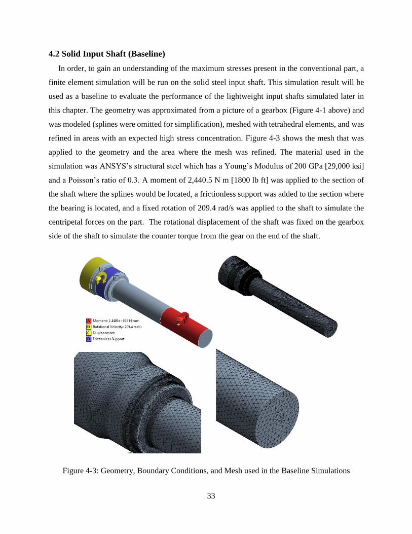
4.2 Solid Input Shaft (Baseline)
In order, to gain an understanding of the maximum stresses present in the conventional part, a
finite element simulation will be run on the solid steel input shaft. This simulation result will be
used as a baseline to evaluate the performance of the lightweight input shafts simulated later in
this chapter. The geometry was approximated from a picture of a gearbox (Figure 4-1 above) and
was modeled (splines were omitted for simplification), meshed with tetrahedral elements, and was
refined in areas with an expected high stress concentration. Figure 4-3 shows the mesh that was
applied to the geometry and the area where the mesh was refined. The material used in the
simulation was ANSYS’s structural steel which has a Young’s Modulus of 200 GPa [29,000 ksi]
and a Poisson’s ratio of 0.3. A moment of 2,440.5 N m [1800 lb ft] was applied to the section of
the shaft where the splines would be located, a frictionless support was added to the section where
the bearing is located, and a fixed rotation of 209.4 rad/s was applied to the shaft to simulate the
centripetal forces on the part. The rotational displacement of the shaft was fixed on the gearbox
side of the shaft to simulate the counter torque from the gear on the end of the shaft.
Figure 4-3: Geometry, Boundary Conditions, and Mesh used in the Baseline Simulations

34
Figure 4-4 and Figure 4-5 below show the results of the simulation of the baseline input shaft.
The maximum stress from the simulation is 645 MPa [93.5 ksi]. This stress concentration occurs
at the radius of the flange due to the diameter change. Most of the stress on the shaft is concentrated
along the outer diameter, with very little stress being located in the center, implying that material
in the shaft’s center increases the weight of the shaft without adding significant strength to the
part. The weight of the input shaft could be reduced by applying weight reduction techniques such
as hollowing out the center, or filling the center with a lighter metal material.
Figure 4-4: Stress [MPa] in the Solid Input Shaft
35
Figure 4-5: Cross Sectional View of the Stress Distribution in the Input Shaft
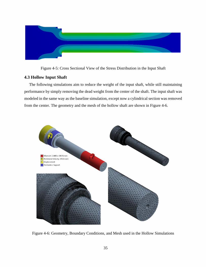
4.3 Hollow Input Shaft
The following simulations aim to reduce the weight of the input shaft, while still maintaining
performance by simply removing the dead weight from the center of the shaft. The input shaft was
modeled in the same way as the baseline simulation, except now a cylindrical section was removed
from the center. The geometry and the mesh of the hollow shaft are shown in Figure 4-6.
Figure 4-6: Geometry, Boundary Conditions, and Mesh used in the Hollow Simulations
36
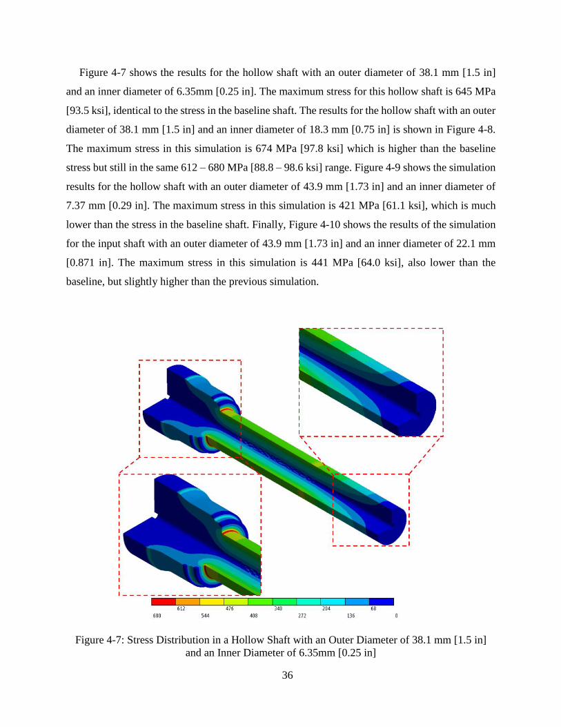
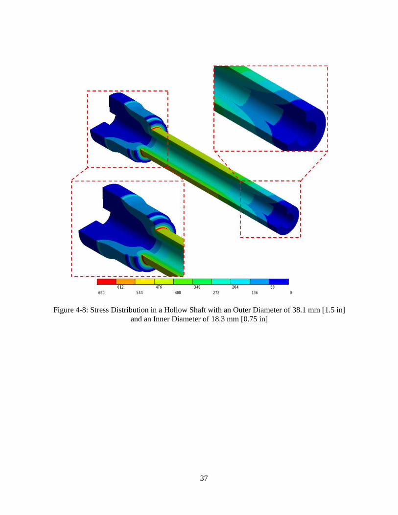
Figure 4-7 shows the results for the hollow shaft with an outer diameter of 38.1 mm [1.5 in]
and an inner diameter of 6.35mm [0.25 in]. The maximum stress for this hollow shaft is 645 MPa
[93.5 ksi], identical to the stress in the baseline shaft. The results for the hollow shaft with an outer
diameter of 38.1 mm [1.5 in] and an inner diameter of 18.3 mm [0.75 in] is shown in Figure 4-8.
The maximum stress in this simulation is 674 MPa [97.8 ksi] which is higher than the baseline
stress but still in the same 612 – 680 MPa [88.8 – 98.6 ksi] range. Figure 4-9 shows the simulation
results for the hollow shaft with an outer diameter of 43.9 mm [1.73 in] and an inner diameter of
7.37 mm [0.29 in]. The maximum stress in this simulation is 421 MPa [61.1 ksi], which is much
lower than the stress in the baseline shaft. Finally, Figure 4-10 shows the results of the simulation
for the input shaft with an outer diameter of 43.9 mm [1.73 in] and an inner diameter of 22.1 mm
[0.871 in]. The maximum stress in this simulation is 441 MPa [64.0 ksi], also lower than the
baseline, but slightly higher than the previous simulation.
Figure 4-7: Stress Distribution in a Hollow Shaft with an Outer Diameter of 38.1 mm [1.5 in]
and an Inner Diameter of 6.35mm [0.25 in]
37
Figure 4-8: Stress Distribution in a Hollow Shaft with an Outer Diameter of 38.1 mm [1.5 in]
and an Inner Diameter of 18.3 mm [0.75 in]

38
Figure 4-9: Stress Distribution in a Hollow Shaft with an Outer Diameter of 43.9 mm [1.73 in]
and an Inner Diameter of 7.37 mm [0.29 in]

39
Figure 4-10: Stress Distribution in a Hollow Shaft with an Outer Diameter of 43.9 mm [1.73 in]
and an Inner Diameter of 22.1 mm [0.871 in]
A parametric study was run to determine the potential weight savings of a hollow input shaft.
The study varied the outer diameter and wall thickness of the shaft to see how the stress and weight
were affected.
Figure 4-11 shows the maximum stress in the hollow input shaft as a function of the aspect ratio
of the hole, (wall thickness to outer diameter) for three different values of the shaft’s outer
diameter. It can be seen that at any given aspect ratio, the smaller outer diameter shafts experience
a higher maximum stress, while the larger outer diameter shafts experience a lower maximum
stress. It can also be seen that for each outer diameter, the maximum stress experienced decreases

40
exponentially as the wall thickness to outer diameter ratio increases (as the inner diameter hole
becomes smaller).
Figure 4-12 shows the mass of the input shaft as a function of that same aspect ratio. It can be
seen that the larger outer diameter shafts have more mass than the smaller outer diameter shafts at
any given aspect ratio. It is also shown that for each outer diameter, as the aspect ratio increases
(the hole gets smaller), the mass also increases. By using both graphs together the potential weight
savings for the hollow input shaft can be determined. First the dimensions of the hollow shaft with
equal performance to the solid steel shaft must be determined, and then the weight of this geometry
must be determined. Based on these results, a potential weight savings of 1.75 kg (3.85 lbs) or
more can be achieved, which is a savings of 48%.

41
Figure 4-11: Maximum Stress in the Input Shaft as a Function of Hole Aspect Ratio for
Various Diameter Shafts
Figure 4-12: Mass of the Input Shaft as a Function of Hole Aspect Ratio for Various Diameter
Shafts
0
200
400
600
800
1000
1200
0 0.1 0.2 0.3 0.4 0.5
Stre
ss [
MPa
]
Wall Thickness/Diameter
OD 1.5 in [38.1 mm]OD 1.73 in [43.942 mm]OD 1.96 in [49.784 mm]Baseline Stress [MPa]
0
1
2
3
4
5
6
0 0.1 0.2 0.3 0.4 0.5
Mas
s [k
g]
Wall Thickness/Diameter
OD 1.5 in [38.1 mm]OD 1.73 in [43.942 mm]OD 1.96 in [49.784 mm]Baseline Mass [kg]

42
4.4 Bimetallic Input Shaft
For the bimetallic simulations, the two materials used were steel for the outer shaft material and
aluminum for the inner shaft material. The same steel used for the baseline and hollow simulation
was used here. The aluminum material had a Young’s Modulus of 71 GPa [10,300 ksi] and a
Poisson’s ratio of 0.33. These shafts were modeled in the same way as the hollow shafts, but
instead of leaving the cylindrical section in the center empty, it was filled in with the aluminum
material, while the outer geometry of the shaft had the steel properties applied. The geometry and
the mesh can be seen in Figure 4-13 below.
Figure 4-13: Geometry, Boundary Conditions, and Mesh used in the Bimetallic Simulations
Figure 4-14 shows the stress distribution for the bimetallic shaft with an outer diameter of 38.1
mm [1.5 in] and an inner diameter of 6.35mm [0.25 in]. The maximum stress in this simulation is
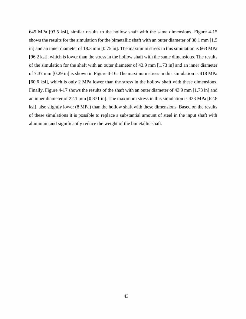
43
645 MPa [93.5 ksi], similar results to the hollow shaft with the same dimensions. Figure 4-15
shows the results for the simulation for the bimetallic shaft with an outer diameter of 38.1 mm [1.5
in] and an inner diameter of 18.3 mm [0.75 in]. The maximum stress in this simulation is 663 MPa
[96.2 ksi], which is lower than the stress in the hollow shaft with the same dimensions. The results
of the simulation for the shaft with an outer diameter of 43.9 mm [1.73 in] and an inner diameter
of 7.37 mm [0.29 in] is shown in Figure 4-16. The maximum stress in this simulation is 418 MPa
[60.6 ksi], which is only 2 MPa lower than the stress in the hollow shaft with these dimensions.
Finally, Figure 4-17 shows the results of the shaft with an outer diameter of 43.9 mm [1.73 in] and
an inner diameter of 22.1 mm [0.871 in]. The maximum stress in this simulation is 433 MPa [62.8
ksi], also slightly lower (8 MPa) than the hollow shaft with these dimensions. Based on the results
of these simulations it is possible to replace a substantial amount of steel in the input shaft with
aluminum and significantly reduce the weight of the bimetallic shaft.
44
Figure 4-14: Stress Distribution in a Bimetallic Shaft with an Outer Diameter of 38.1 mm [1.5 in]
and an Inner Diameter of 6.35mm [0.25 in]
45
Figure 4-15: Stress Distribution in a Bimetallic Shaft with an Outer Diameter of 38.1 mm [1.5 in]
and an Inner Diameter of 18.3 mm [0.75 in]
46
Figure 4-16: Stress Distribution in a Bimetallic Shaft with an Outer Diameter of 43.9 mm [1.73
in] and an Inner Diameter of 7.37 mm [0.29 in]
47
Figure 4-17: Stress Distribution in a Bimetallic Shaft with an Outer Diameter of 43.9 mm [1.73
in] and an Inner Diameter of 22.1 mm [0.871 in]
48
Figure 4-18: Maximum Stress in the Input Shaft as a Function of Hole Aspect Ratio for Various
Diameter Shafts
Figure 4-19: Mass of the Input Shaft as a Function of Hole Aspect Ratio for Various Diameter
Shafts
0
100
200
300
400
500
600
700
800
900
0 0.1 0.2 0.3 0.4 0.5
Stre
ss [
MP
a]
Wall Thickness/Diameter
OD 1.5 in [38.1 mm]OD 1.73 in [43.942 mm]OD 1.96 in [49.784 mm]Baseline Stress [MPa]
0
1
2
3
4
5
6
0 0.1 0.2 0.3 0.4 0.5
Mas
s [k
g]
Wall Thickness/Diameter
OD 1.5 in [38.1 mm]OD 1.73 in [43.942 mm]OD 1.96 in [49.784 mm]Baseline Mass [kg]

49
Another parametric study was performed on the bimetallic shafts, investigating the same
parameters as the study done on the hollow shafts.
Figure 4-18 shows the maximum stress in the bimetallic input shaft as a function of the aspect
ratio of the hole for the three different outer diameter shafts. It can be seen that for each aspect
ratio, the smaller outer diameter shafts experience a higher maximum stress, while the larger outer
diameter shafts experience a lower maximum stress, similar to the results of the hollow shafts. It
can also be seen that for each outer diameter, the maximum stress experienced decreases
exponentially as the wall thickness to outer diameter ratio increases, also similar to the hollow
shaft results.
Figure 4-19 shows the mass of the input shaft as a function of the hole aspect ratio. It can be
seen that the larger outer diameter shafts have more mass than the smaller outer diameter shafts at
any given aspect ratio and that for each outer diameter, as the aspect ratio increases, the mass also
increases. These results follow the same trends observed in the parametric study done on the
hollow shafts. Based on the amount of weight which can be saved by switching from the solid
steel shafts to the bimetallic shafts is about 0.9 kg [2 lbs] or 25%.
4.5 Conclusion
The mass of a single input shaft is small (only about 3.7 kg or 8.14 lbs), so the total weight
which can be saved by switching to a light weight design is also small. However, the reduction in
the shaft’s weight is an important part of a larger total weight reduction which can be achieved
when considering all of the small savings in the gearbox. The finite element studies carried out
revealed that the weight of the shaft could be reduced by 1.75 kg [3.85 lbs] if hollow geometry
was employed and 0.9 kg [2 lbs] if the bimetallic variant of the shaft was used. These savings
would require the diameter of the shaft to be increased by a mere 15%. Greater savings could be
expected for shafts with larger outer diameters. The small weight savings achievable on the input
shaft must be weighed against the cost of updating the manufacturing process to create the light
weight components.
50
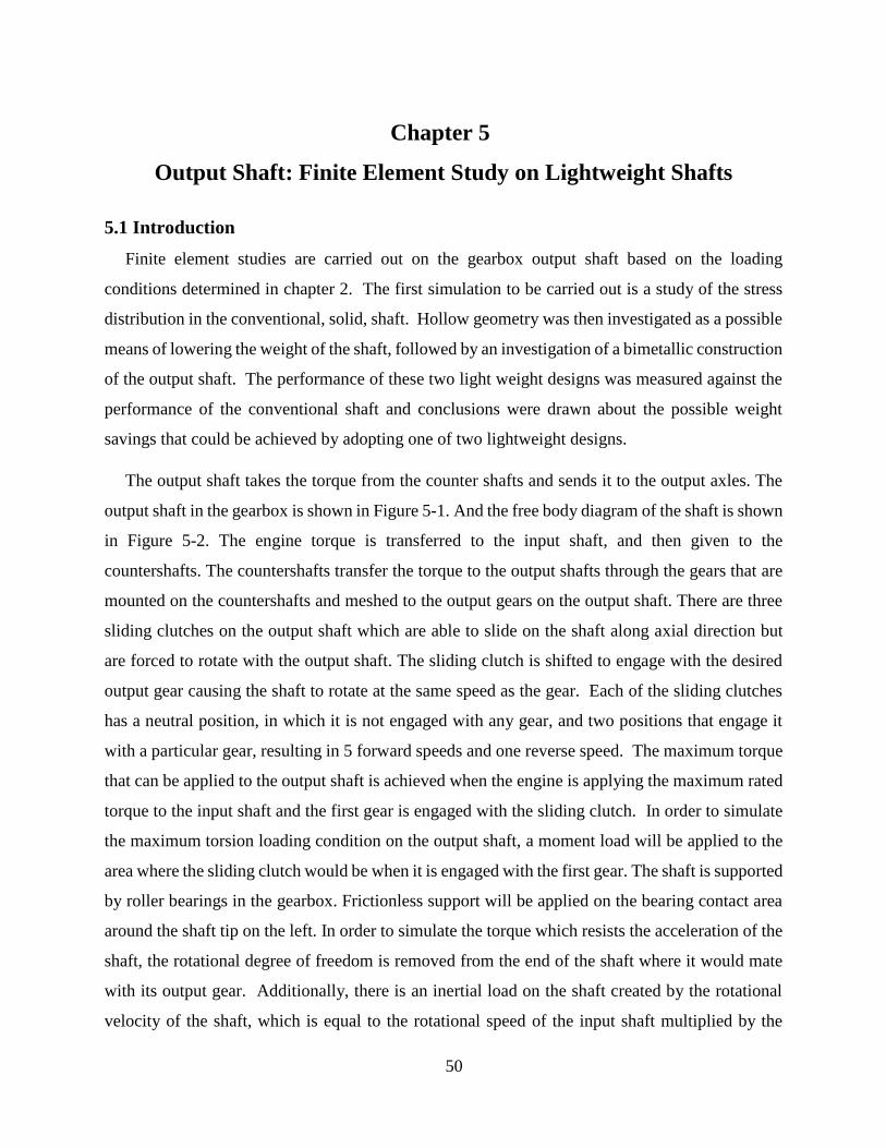
Chapter 5
Output Shaft: Finite Element Study on Lightweight Shafts
5.1 Introduction
Finite element studies are carried out on the gearbox output shaft based on the loading
conditions determined in chapter 2. The first simulation to be carried out is a study of the stress
distribution in the conventional, solid, shaft. Hollow geometry was then investigated as a possible
means of lowering the weight of the shaft, followed by an investigation of a bimetallic construction
of the output shaft. The performance of these two light weight designs was measured against the
performance of the conventional shaft and conclusions were drawn about the possible weight
savings that could be achieved by adopting one of two lightweight designs.
The output shaft takes the torque from the counter shafts and sends it to the output axles. The
output shaft in the gearbox is shown in Figure 5-1. And the free body diagram of the shaft is shown
in Figure 5-2. The engine torque is transferred to the input shaft, and then given to the
countershafts. The countershafts transfer the torque to the output shafts through the gears that are
mounted on the countershafts and meshed to the output gears on the output shaft. There are three
sliding clutches on the output shaft which are able to slide on the shaft along axial direction but
are forced to rotate with the output shaft. The sliding clutch is shifted to engage with the desired
output gear causing the shaft to rotate at the same speed as the gear. Each of the sliding clutches
has a neutral position, in which it is not engaged with any gear, and two positions that engage it
with a particular gear, resulting in 5 forward speeds and one reverse speed. The maximum torque
that can be applied to the output shaft is achieved when the engine is applying the maximum rated
torque to the input shaft and the first gear is engaged with the sliding clutch. In order to simulate
the maximum torsion loading condition on the output shaft, a moment load will be applied to the
area where the sliding clutch would be when it is engaged with the first gear. The shaft is supported
by roller bearings in the gearbox. Frictionless support will be applied on the bearing contact area
around the shaft tip on the left. In order to simulate the torque which resists the acceleration of the
shaft, the rotational degree of freedom is removed from the end of the shaft where it would mate
with its output gear. Additionally, there is an inertial load on the shaft created by the rotational
velocity of the shaft, which is equal to the rotational speed of the input shaft multiplied by the

51
specific gear ratio. Since there are three balanced countershafts, the bending loads that result from
the meshing of the gears of the countershafts with the gear on the output shaft cancel out and only
a net torsional load is applied to the output shaft.
Figure 5-1: The output shaft in the truck engine
Figure 5-2: Output shaft FBD
52
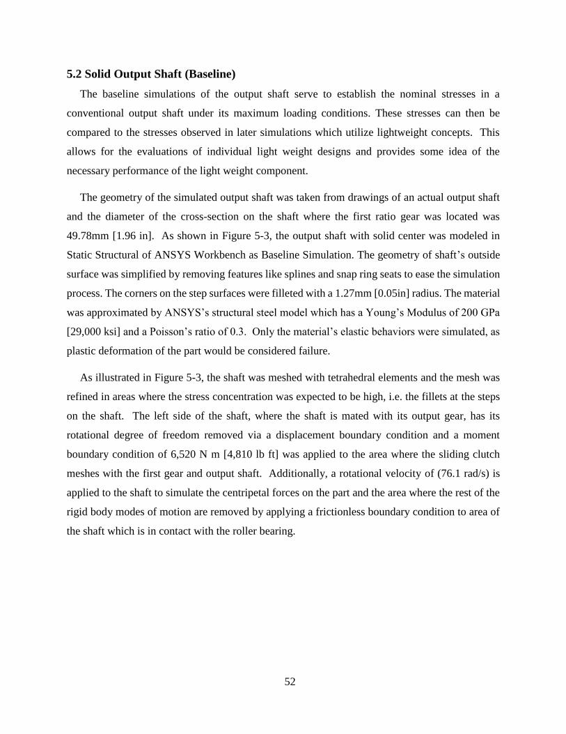
5.2 Solid Output Shaft (Baseline)
The baseline simulations of the output shaft serve to establish the nominal stresses in a
conventional output shaft under its maximum loading conditions. These stresses can then be
compared to the stresses observed in later simulations which utilize lightweight concepts. This
allows for the evaluations of individual light weight designs and provides some idea of the
necessary performance of the light weight component.
The geometry of the simulated output shaft was taken from drawings of an actual output shaft
and the diameter of the cross-section on the shaft where the first ratio gear was located was
49.78mm [1.96 in]. As shown in Figure 5-3, the output shaft with solid center was modeled in
Static Structural of ANSYS Workbench as Baseline Simulation. The geometry of shaft’s outside
surface was simplified by removing features like splines and snap ring seats to ease the simulation
process. The corners on the step surfaces were filleted with a 1.27mm [0.05in] radius. The material
was approximated by ANSYS’s structural steel model which has a Young’s Modulus of 200 GPa
[29,000 ksi] and a Poisson’s ratio of 0.3. Only the material’s elastic behaviors were simulated, as
plastic deformation of the part would be considered failure.
As illustrated in Figure 5-3, the shaft was meshed with tetrahedral elements and the mesh was
refined in areas where the stress concentration was expected to be high, i.e. the fillets at the steps
on the shaft. The left side of the shaft, where the shaft is mated with its output gear, has its
rotational degree of freedom removed via a displacement boundary condition and a moment
boundary condition of 6,520 N m [4,810 lb ft] was applied to the area where the sliding clutch
meshes with the first gear and output shaft. Additionally, a rotational velocity of (76.1 rad/s) is
applied to the shaft to simulate the centripetal forces on the part and the area where the rest of the
rigid body modes of motion are removed by applying a frictionless boundary condition to area of
the shaft which is in contact with the roller bearing.

53
Figure 5-3: Geometry, Boundary Conditions, and Mesh used in the Baseline Simulations of the
Output Shaft
After the completion of the simulation the stress contours were plotted as shown in Figure 5-4.
Due to numerical error cause by the simplification of the real loading conditions to the boundary
conditions used in the finite element simulations, specifically the fixed rotation condition, the
stress was higher around the transitions from the free surface to the fixed surface on the shaft.
Ignoring the numerical error around the fixed boundary condition, the maximum stress on the
output shaft was about 466 MPa [67.6 ksi]. The shaft only sees stress in a relatively localized area
because only the first gear is engaged. If, for instance, the fourth gear were engaged, instead of
the first, the entire shaft would be subjected to stress.
As was the case in the previous chapters, the stresses in the output shaft are concentrated on the
outer diameter of the shaft and that the stress in the middle of the shaft is almost zero, as shown in
Figure 5-4. Thus the material in the middle of the shaft increases the weight of the part without
contributing significantly to its strength. The weight of the shaft could be significantly reduced by
removing this parasitic material from the inside of the shaft or by replacing it with a lower density
material.

54
Figure 5-4: Stress [MPa] in the Solid Output Shaft
5.3 Hollow Output Shaft
The following simulations demonstrate how the performance of the shaft can be maintained
while significantly reducing the weight of the part by removing the parasitic material from the
center of the shaft. As shown in Figure 5-5, for the purposes of these simulations, the shaft was
hollowed by removing a section of material from the center of the output shaft which was similar
to the outer diameter of the shaft. The ratios between the outside diameters and inside diameters
for each main cross section are kept the same (𝐷𝑜 𝐷𝑖⁄ = 𝐶𝑜𝑛𝑠𝑡𝑎𝑛𝑡). In practice this would be
difficult to fabricate as a single part, as it would require the forged blank to have a drilled hole
with multiple diameters which would be time consuming and difficult for machining. A possible
and attractive way to fabricate this shaft would be to start with a thick tube and forge the tube into
shafts with the correct inner to outer diameter ratios.
The first hollow shaft simulation which was carried out had the same outside dimensions as the
baseline output shaft, but had a 6.35mm [0.25 in] hole on the large diameter section of the part
where the first ratio gear was connected. The stress distribution in this part is given in Figure 5-6.
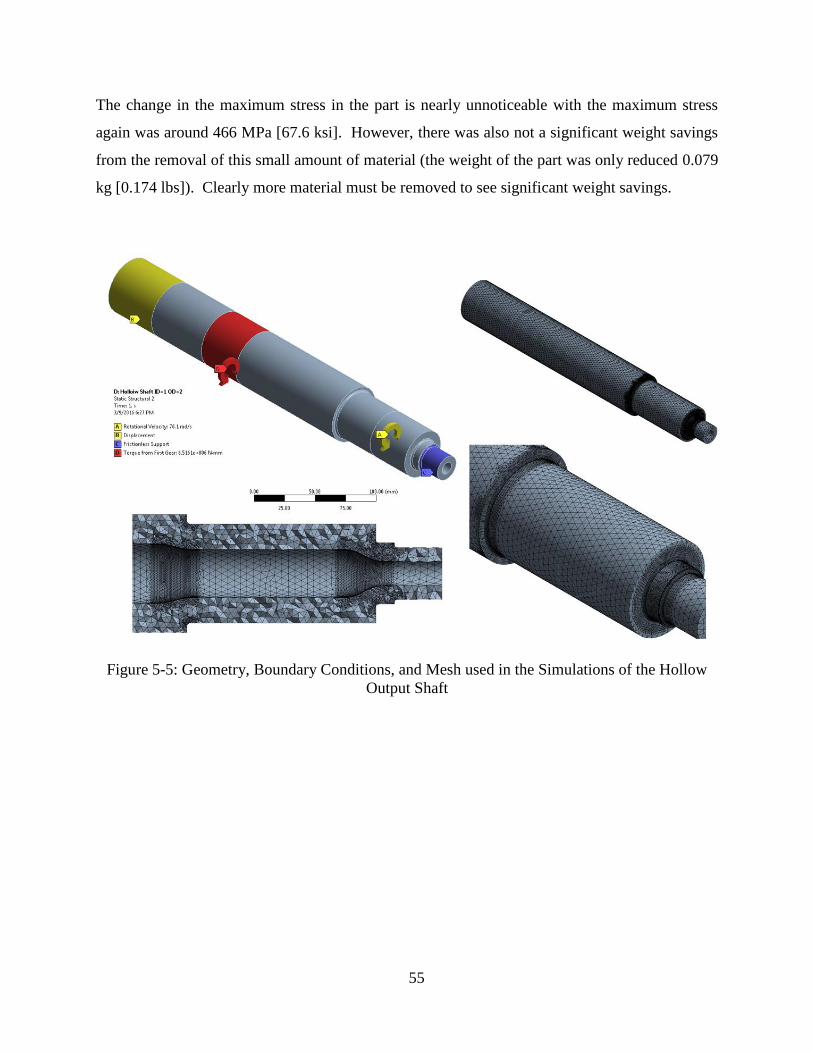
55
The change in the maximum stress in the part is nearly unnoticeable with the maximum stress
again was around 466 MPa [67.6 ksi]. However, there was also not a significant weight savings
from the removal of this small amount of material (the weight of the part was only reduced 0.079
kg [0.174 lbs]). Clearly more material must be removed to see significant weight savings.
Figure 5-5: Geometry, Boundary Conditions, and Mesh used in the Simulations of the Hollow
Output Shaft
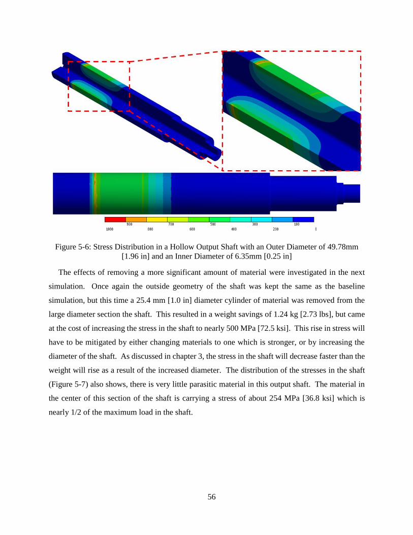
56
Figure 5-6: Stress Distribution in a Hollow Output Shaft with an Outer Diameter of 49.78mm
[1.96 in] and an Inner Diameter of 6.35mm [0.25 in]
The effects of removing a more significant amount of material were investigated in the next
simulation. Once again the outside geometry of the shaft was kept the same as the baseline
simulation, but this time a 25.4 mm [1.0 in] diameter cylinder of material was removed from the
large diameter section the shaft. This resulted in a weight savings of 1.24 kg [2.73 lbs], but came
at the cost of increasing the stress in the shaft to nearly 500 MPa [72.5 ksi]. This rise in stress will
have to be mitigated by either changing materials to one which is stronger, or by increasing the
diameter of the shaft. As discussed in chapter 3, the stress in the shaft will decrease faster than the
weight will rise as a result of the increased diameter. The distribution of the stresses in the shaft
(Figure 5-7) also shows, there is very little parasitic material in this output shaft. The material in
the center of this section of the shaft is carrying a stress of about 254 MPa [36.8 ksi] which is
nearly 1/2 of the maximum load in the shaft.
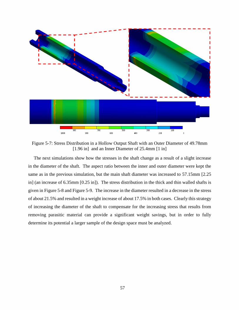
57
Figure 5-7: Stress Distribution in a Hollow Output Shaft with an Outer Diameter of 49.78mm
[1.96 in] and an Inner Diameter of 25.4mm [1 in]
The next simulations show how the stresses in the shaft change as a result of a slight increase
in the diameter of the shaft. The aspect ratio between the inner and outer diameter were kept the
same as in the previous simulation, but the main shaft diameter was increased to 57.15mm [2.25
in] (an increase of 6.35mm [0.25 in]). The stress distribution in the thick and thin walled shafts is
given in Figure 5-8 and Figure 5-9. The increase in the diameter resulted in a decrease in the stress
of about 21.5% and resulted in a weight increase of about 17.5% in both cases. Clearly this strategy
of increasing the diameter of the shaft to compensate for the increasing stress that results from
removing parasitic material can provide a significant weight savings, but in order to fully
determine its potential a larger sample of the design space must be analyzed.

58
Figure 5-8: Stress Distribution in a Hollow Output Shaft with an Outer Diameter of 57.15mm
[2.25 in] and an Inner Diameter of 7.14mm [0.281 in]
Figure 5-9: Stress Distribution in a Hollow Output Shaft with an Outer Diameter of 57.15mm
[2.25 in] and an Inner Diameter of 28.58mm [1.125 in]

59
To determine the potential weight savings of a hollow output shaft, a parametric study was run
which examined the effects of varying the outer diameter and wall thickness to outer diameter ratio
of the output shaft on the maximum stress in the shaft and the weight of the shaft. Figure 3-9
demonstrates how the stress in the shaft changes with respect to the stress in the baseline study as
the wall thickness ratio and shaft diameter change. The point where the stress curves for the
various diameters are equal to the baseline stress represents the wall thickness ratio that will create
a shaft with equal performance to the conventional, solid shaft for the shaft diameter corresponding
to the particular curve. These wall thickness ratios can then be used in conjunction with Figure
3-10 to determine the weight savings of each of the equal performance designs.
The stress in the shaft is clearly not sensitive to small holes in the shaft, but as the hole increases
in diameter it removes material that is responsible for carrying an ever increasing amount of the
load, resulting in rapidly rising stresses as the wall thickness ratio approaches zero. Additionally,
increases in the outer diameter of the shaft serve only to shift the stress curve down, without
significantly affecting the shape of the curve. The weight of the equally performing shaft tends to
decrease as the outer diameter of the shaft is allowed to increase, so the designer will have to weigh
the cost of reduced weight against the drawback of a less compact shaft. Based on the study
performed the weight of the axle shaft could be reduced by 35-44% by switching to a hollow shaft,
depending on the outer diameter of the replacement shaft. This is a savings of 1.7 to 2.2 kg [3.74
to 4.84 lbs] for the output shaft.

60
Figure 5-10: Maximum Stress in the Hollow Output Shaft as a Function of Hole Aspect Ratio
for Various Diameter Shafts
Figure 5-11: Mass of the Hollow Output Shaft as a Function of Hole Aspect Ratio for Various
Diameter Shafts
5.4 Bimetallic Output Shaft
The following simulations demonstrate how the performance of the shaft can be maintained
while significantly reducing the weight of the part by replacing the parasitic material in the center
with light metals like aluminum. As shown in Figure 5-12, the geometry of the bimetallic output
0
100
200
300
400
500
600
700
800
0 0.1 0.2 0.3 0.4 0.5
Stre
ss [
MPa
]
Wall Thickness/Diameter
OD 2in [50.8mm]OD 2.125in [54.0mm]OD 2.25in [57.2mm]Baseline [MPa]
0
1
2
3
4
5
6
7
0 0.1 0.2 0.3 0.4 0.5
Mas
s [k
g]
Wall Thickness/Diameter
OD 2in [50.8mm]OD 2.125in [54.0mm]OD 2.25in [57.2mm]Baseline [kg]
61
shaft is nearly identical to the hollow shaft geometry, except for the empty portion of the shaft is
replaced with an aluminum material, which was assumed to have a Young’s Modulus of 71 GPa
[10,300 ksi] and a Poisson’s ratio of 0.33. This would be a challenging part to fabricate as the two
parts must be well bonded so that the core can assist in carrying the torsional load applied to the
shaft. It is possible that a high quality bond could be established by forging the shaft out of a
bimetallic billet, which could make the bond as strong as the shear strength of the weaker material.
The first bimetallic simulation which was carried out had the same outside dimensions as the
baseline output shaft, but had a 6.35mm [0.25 in] aluminum core in large diameter portion of the
shaft. As a reminder, the geometry of the aluminum core is identical to the geometry of the hole
in the hollow shaft simulations. The stress distribution in this part is given in Figure 5-13. The
change in the maximum stress in the part is nearly unnoticeable with the maximum stress again
was around 466 MPa [67.6 ksi] range. However there was also not a significant weight savings
from replacing this small amount of parasitic steel material with aluminum (the weight of the part
was only reduced 0.05 kg [0.11 lbs]). Clearly more material can be replaced to see significant
weight savings.
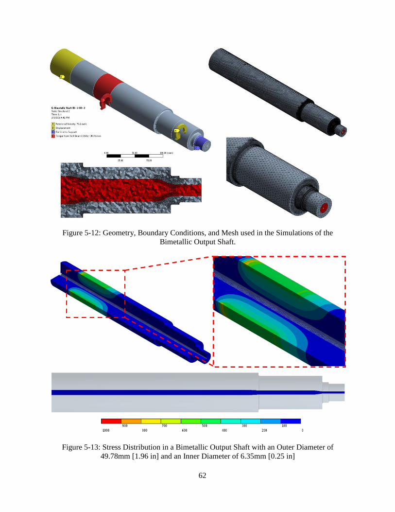
62
Figure 5-12: Geometry, Boundary Conditions, and Mesh used in the Simulations of the
Bimetallic Output Shaft.
Figure 5-13: Stress Distribution in a Bimetallic Output Shaft with an Outer Diameter of
49.78mm [1.96 in] and an Inner Diameter of 6.35mm [0.25 in]
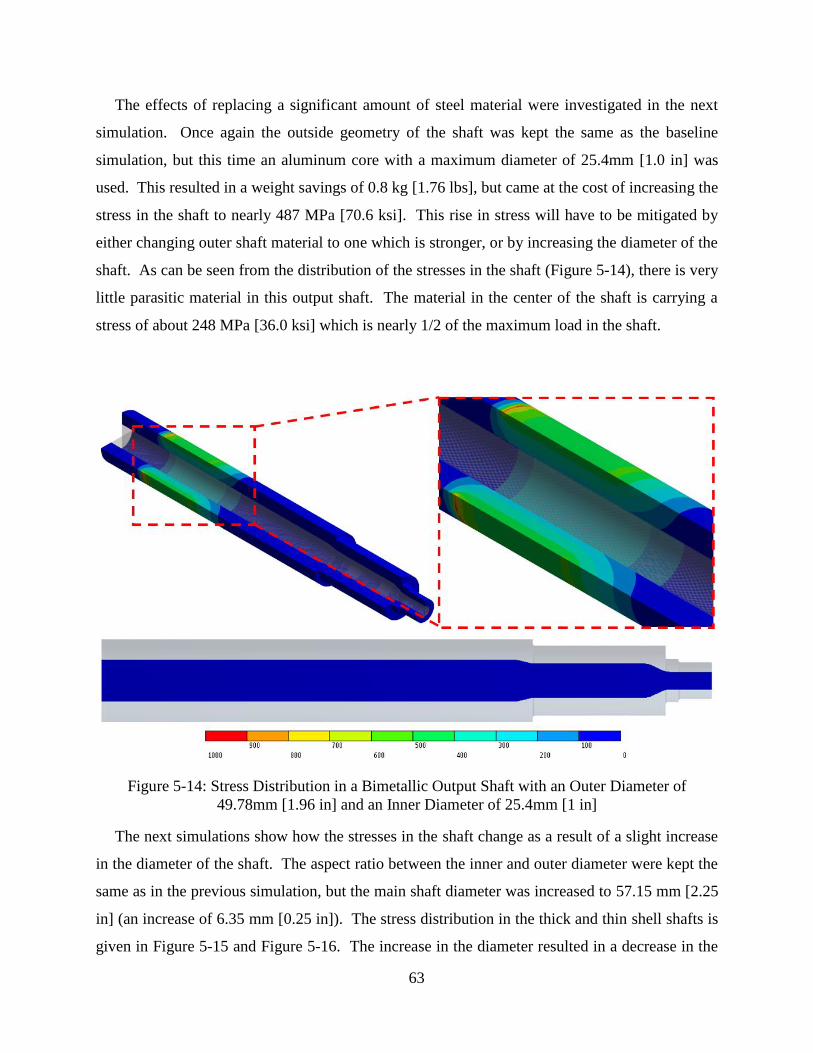
63
The effects of replacing a significant amount of steel material were investigated in the next
simulation. Once again the outside geometry of the shaft was kept the same as the baseline
simulation, but this time an aluminum core with a maximum diameter of 25.4mm [1.0 in] was
used. This resulted in a weight savings of 0.8 kg [1.76 lbs], but came at the cost of increasing the
stress in the shaft to nearly 487 MPa [70.6 ksi]. This rise in stress will have to be mitigated by
either changing outer shaft material to one which is stronger, or by increasing the diameter of the
shaft. As can be seen from the distribution of the stresses in the shaft (Figure 5-14), there is very
little parasitic material in this output shaft. The material in the center of the shaft is carrying a
stress of about 248 MPa [36.0 ksi] which is nearly 1/2 of the maximum load in the shaft.
Figure 5-14: Stress Distribution in a Bimetallic Output Shaft with an Outer Diameter of
49.78mm [1.96 in] and an Inner Diameter of 25.4mm [1 in]
The next simulations show how the stresses in the shaft change as a result of a slight increase
in the diameter of the shaft. The aspect ratio between the inner and outer diameter were kept the
same as in the previous simulation, but the main shaft diameter was increased to 57.15 mm [2.25
in] (an increase of 6.35 mm [0.25 in]). The stress distribution in the thick and thin shell shafts is
given in Figure 5-15 and Figure 5-16. The increase in the diameter resulted in a decrease in the
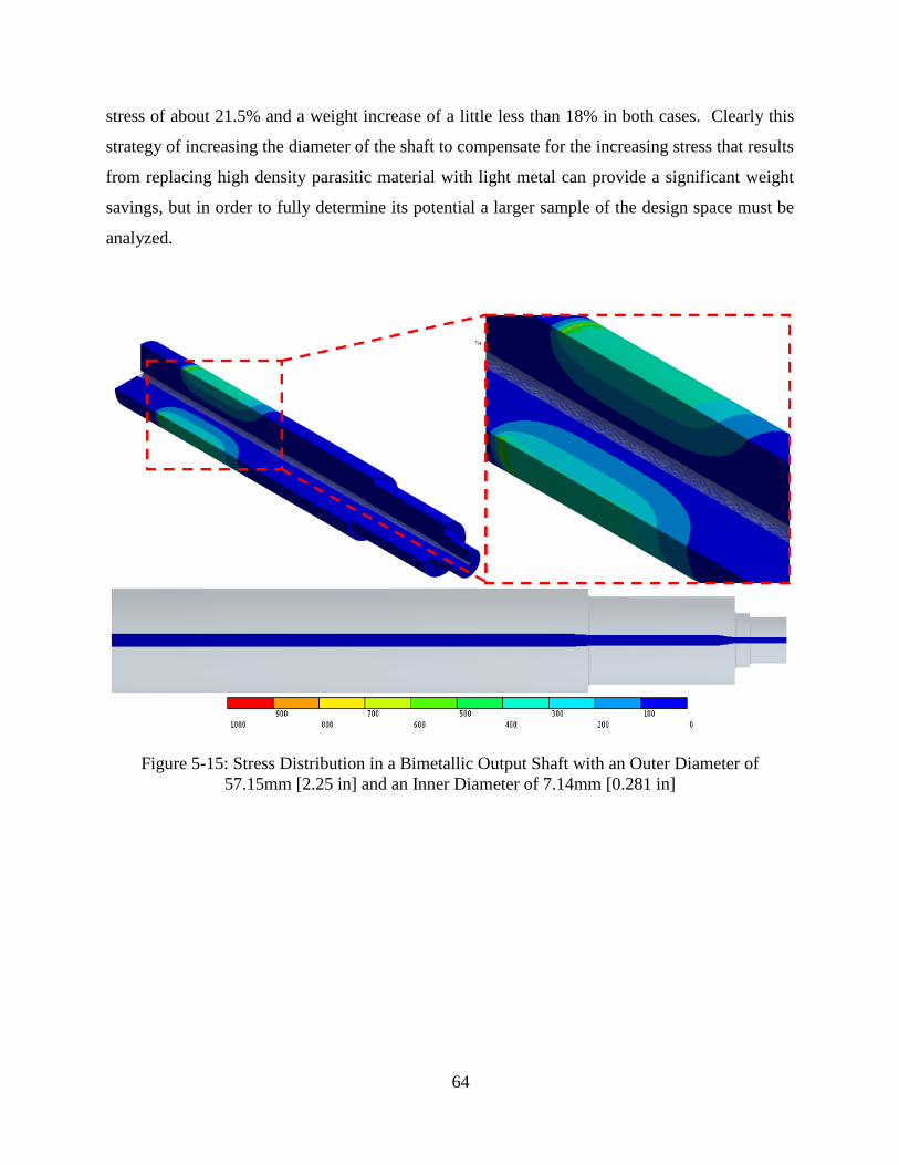
64
stress of about 21.5% and a weight increase of a little less than 18% in both cases. Clearly this
strategy of increasing the diameter of the shaft to compensate for the increasing stress that results
from replacing high density parasitic material with light metal can provide a significant weight
savings, but in order to fully determine its potential a larger sample of the design space must be
analyzed.
Figure 5-15: Stress Distribution in a Bimetallic Output Shaft with an Outer Diameter of
57.15mm [2.25 in] and an Inner Diameter of 7.14mm [0.281 in]
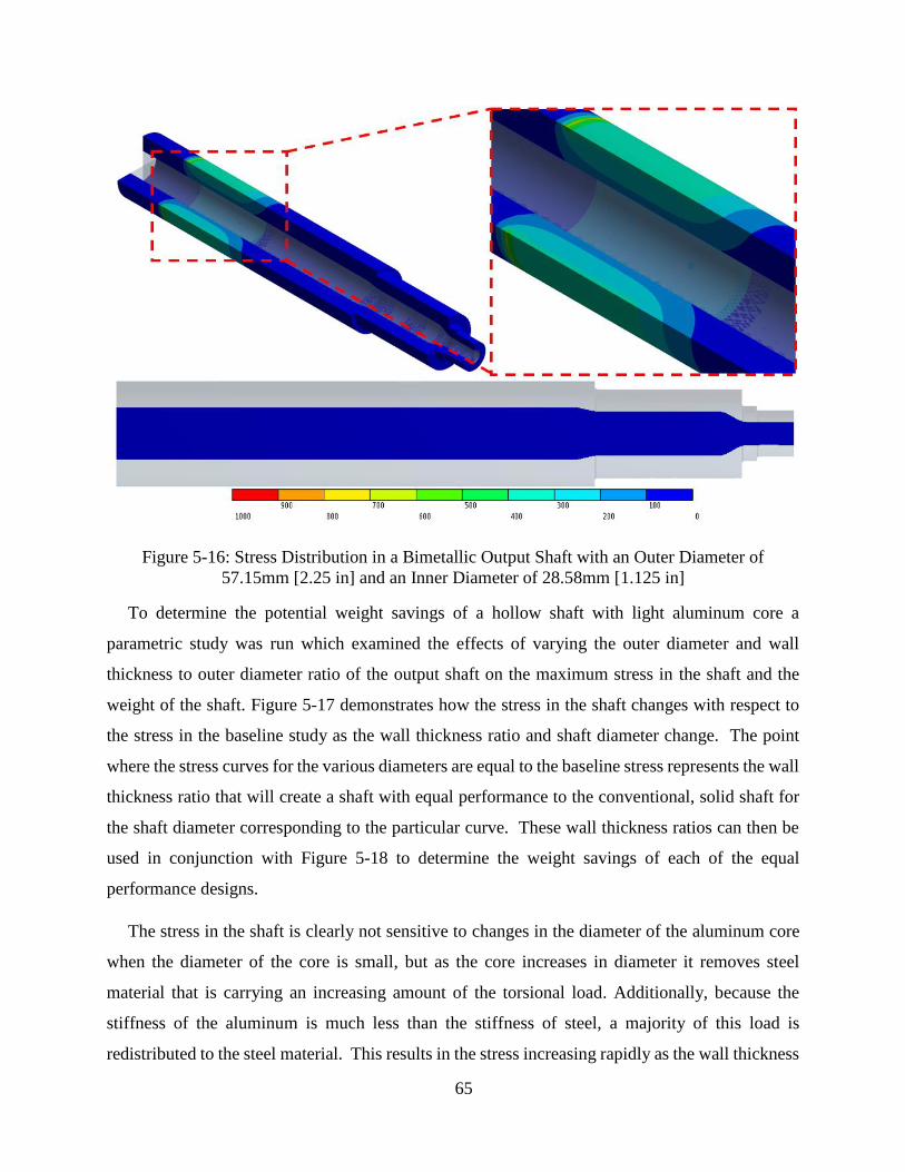
65
Figure 5-16: Stress Distribution in a Bimetallic Output Shaft with an Outer Diameter of
57.15mm [2.25 in] and an Inner Diameter of 28.58mm [1.125 in]
To determine the potential weight savings of a hollow shaft with light aluminum core a
parametric study was run which examined the effects of varying the outer diameter and wall
thickness to outer diameter ratio of the output shaft on the maximum stress in the shaft and the
weight of the shaft. Figure 5-17 demonstrates how the stress in the shaft changes with respect to
the stress in the baseline study as the wall thickness ratio and shaft diameter change. The point
where the stress curves for the various diameters are equal to the baseline stress represents the wall
thickness ratio that will create a shaft with equal performance to the conventional, solid shaft for
the shaft diameter corresponding to the particular curve. These wall thickness ratios can then be
used in conjunction with Figure 5-18 to determine the weight savings of each of the equal
performance designs.
The stress in the shaft is clearly not sensitive to changes in the diameter of the aluminum core
when the diameter of the core is small, but as the core increases in diameter it removes steel
material that is carrying an increasing amount of the torsional load. Additionally, because the
stiffness of the aluminum is much less than the stiffness of steel, a majority of this load is
redistributed to the steel material. This results in the stress increasing rapidly as the wall thickness

66
ratio approaches zero, but the stress does not approach infinity as it did with the hollow shaft.
Rather, it approaches the stress that a steel would reach as it approached the strain in a 100%
aluminum shaft under the same loading. It is also noted that increases in the outer diameter of the
shaft serve only to shift the stress curve down, without significantly affecting the shape of the
curve. The weight of the equally performing shaft tends to decrease as the outer diameter of the
shaft is allowed to increase, so the designer will have to weigh the cost of reduced weight against
the drawback of a less compact shaft. Based on the study performed the weight of the axle shaft
could be reduced by 26% by switching to a hollow shaft, depending on the outer diameter of the
replacement shaft. This is a savings of 1.29 kg [2.84 lbs] for the output shaft.
Figure 5-17: Maximum Stress in the Bimetallic Output Shaft as a Function of Hole Aspect Ratio
for Various Diameter Shafts
0
100
200
300
400
500
600
700
0 0.1 0.2 0.3 0.4 0.5
Stre
ss [
MPa
]
Wall Thickness/Diameter
OD 2in [50.8mm]OD 2.125in [54.0mm]OD 2.25in [57.2mm]Baseline [MPa]
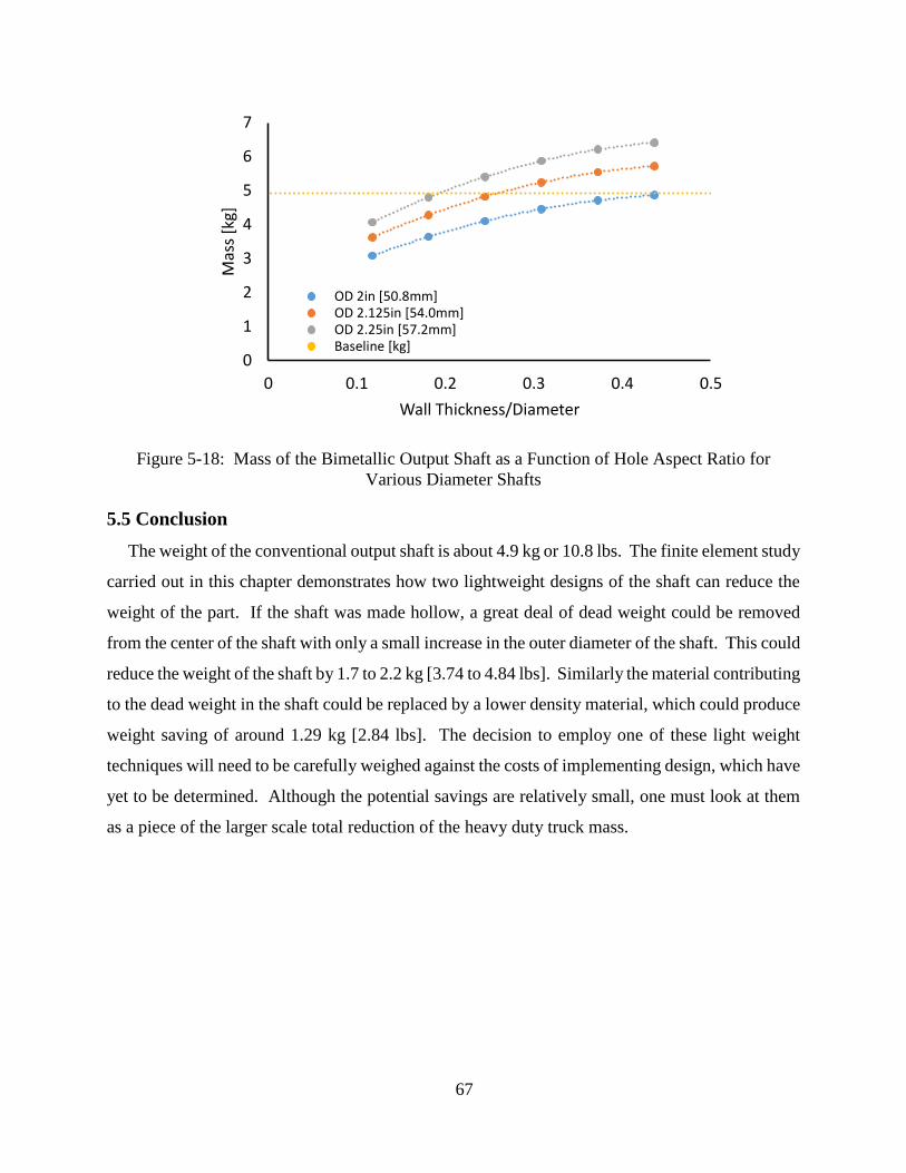
67
Figure 5-18: Mass of the Bimetallic Output Shaft as a Function of Hole Aspect Ratio for
Various Diameter Shafts
5.5 Conclusion
The weight of the conventional output shaft is about 4.9 kg or 10.8 lbs. The finite element study
carried out in this chapter demonstrates how two lightweight designs of the shaft can reduce the
weight of the part. If the shaft was made hollow, a great deal of dead weight could be removed
from the center of the shaft with only a small increase in the outer diameter of the shaft. This could
reduce the weight of the shaft by 1.7 to 2.2 kg [3.74 to 4.84 lbs]. Similarly the material contributing
to the dead weight in the shaft could be replaced by a lower density material, which could produce
weight saving of around 1.29 kg [2.84 lbs]. The decision to employ one of these light weight
techniques will need to be carefully weighed against the costs of implementing design, which have
yet to be determined. Although the potential savings are relatively small, one must look at them
as a piece of the larger scale total reduction of the heavy duty truck mass.
0
1
2
3
4
5
6
7
0 0.1 0.2 0.3 0.4 0.5
Mas
s [k
g]
Wall Thickness/Diameter
OD 2in [50.8mm]OD 2.125in [54.0mm]OD 2.25in [57.2mm]Baseline [kg]

68
Chapter 6
Countershaft: Finite Element Study Light Weight Shafts
6.1 Introduction
This chapter describes the finite element study carried out on both the conventional countershaft
and two lightweight designs of the countershaft. The loads on the countershaft are detailed in
chapter 2, although due to the triple countershaft layout of the reference gearbox the loads are
lower than those described previously. The first part of the finite element study was to determine
the stress distribution in the conventional, solid countershaft. This information was then used as
a baseline to compare the results of the finite element analysis of the lightweight designs. The two
lightweight designs investigated were a hollow shaft geometry and a bimetallic shaft, which
utilized a low density core material.
The countershaft is a gearbox component which transmits torque from the input shaft to the
output shaft. Gears are fixed to the shaft either through a press fit or machined into the shaft itself,
so that they always rotate at the same speed as the countershaft. Additionally, the gears are always
engaged with their corresponding gears on the input and output shafts. Typically, the input and
output shaft are coaxial and the countershaft rotates next to the shafts on a parallel axis. Heavy
duty vehicle gearboxes come with a large variety of countershaft configurations having as few as
one and as many as three counter shafts. Having multiple countershafts serves two main purposes.
First, because the load being transmitted from the input shaft to the output shaft is divided into
multiple paths, the load on the gear teeth and the counter shaft itself is reduced by a factor of the
number of counter shafts engaged. Second, having multiple countershafts allows the bending
forces from the meshing gears to be balanced in such a way that there is not bending moment on
the input or output shafts. However, bending moments on the countershaft cannot be avoided.
The countershaft in a Mack 10 speed Maxitorque is highlighted in Figure 6-1. This particular
gearbox has three countershafts, a torque rating of 2,440 N m [1,800 lb ft], and the first/sixth gear
ratio (not including the high/low range adjustment) is 2.67. Based on measurements taken of the
shaft the gear ratio between the input shaft and the countershaft is about 1.43 meaning that the
total torque carried by the countershafts is 3,490 N m [2,580 lb ft], or 1,163 N m [858 lb ft] per
shaft. As stated previously there will be bending loads on the counter shaft. These loads can be

69
calculated based on the torque carried by the shaft and the size of the input and output gears. In
this case the input gear and output gear corresponding to first/sixth gear have pitch circle diameters
of about 163 mm [6.43 in] and 96.8 mm [3.81 in], respectively. The circumferential forces on the
gears can be calculated by dividing the torque produced by the gear by the radius of the gear and
the radial forces can be calculated by multiplying the circumferential force by the tangent of the
pressure angle of the gears. Assuming a pressure angle of 20°, the circumferential and radial loads
on the input gear are 14,230 N [3,200 lbf] and 5178 N [1,164 lbf], respectively. The corresponding
loads on the output shaft are 24,060 N [5410 lbf] and 8760 N [1969 lbf], respectively. It is
important to remember that the circumferential loads from the gears must balance the torque on
the shaft, so they will be applied in opposite directions. Additionally, if the gears are helical,
instead of spur gears, the radial load will be slightly different and there will be an axial load on the
shaft as well, due to the additional helix angle on the gear teeth. For the purposes of this
investigation the loading conditions for spur gears will be used because the reference gearbox uses
spur gears. Finally, the shaft has inertial loads corresponding to rotational at speeds of 1400 RPM
and is supported on either end by tapered roller bearings.

70
Figure 6-1: Mack 10 Speed Maxitorque ES T310 Gearbox with Simplified Boundary Conditions
used in Finite Element Analysis
6.2 Solid Countershaft (Baseline)
The geometry of and loads applied to the countershaft in the Mack ES T310 gearbox shown in
Figure 6-1 are summarized in Figure 6-2. In order to establish a baseline from which studies of
light weight countershafts can be compared, a solid shaft with the dimensions shown in Figure 6-2
will be simulated via the finite element method. In addition to the shaft itself, the gears, spacers
and key must simulated. This is because the gears and spacers have no space to slide on the shaft
and will, therefore, serve to help the shaft resist the bending load created by the meshing gears.
The key and keyway on the shaft are simulated because they transmit the load to the shaft unevenly
and may have a significant effect on the stresses in the shaft. Contact conditions between the
various simulated parts are as follows: i) the gears have frictionless contact with each other and
the countershaft, ii) the key is bonded to the gears and the key way in the countershaft. The

71
circumferential and radial loads are applied as force boundary conditions to the outside surfaces
of the input and output gears (this is acceptable because the analysis is focused on the countershaft
and not the gears). The torque on the shaft is applied as a moment on the surface of the input gear
and is countered by a using a displacement boundary condition to prevent the output gear from
turning. The shaft is held in place by two frictionless supports on the ends of the shaft where the
bearing would be placed on the real shaft. The simulated geometry and boundary conditions are
illustrated in Figure 6-3. The mesh used to discretize the shaft, gears, and key is given in Figure
6-4.
Figure 6-2: Geometry and Loading on the Countershaft

72
Figure 6-3: (left) Countershaft with Gears, Spacers, and Key Simulated in the Baseline Finite
Element Analysis (right) Boundary Conditions applied to the Countershaft Assembly
Figure 6-4: Mesh used in the Finite Element Simulation of the Solid Countershaft
After the simulation was run, the stress distribution on the shaft was plotted (Figure 6-5) and
examined. The maximum stress on the shaft was 565 MPa [81.8 ksi] and this stress occurred on
the outer radius of the keyway around the area where the output gear counters the torque produced
by the input gear. The maximum stress elsewhere on the shaft is relatively low (about 110 MPa
[16 ksi]). This is interesting as this stress is much lower than the stresses observed in the

73
simulations of the other parts examined. It is likely that the stresses in the shaft could achieve a
more appreciable fraction of the yield strengths of typical automotive grades of steel if the key
way was removed in favor of a coupling method which produced a smaller stress concentration.
Unlike the studies of the other investigated parts, a cross sectional view of the countershaft shows
a high amount of ‘parasitic’ material on not just in the middle of the shaft, but also in the areas
which are far from the keyway. It is very likely that the shaft’s weight can be reduced without
significantly affecting its strength by removing this material, or replacing it with a lower density
material. Additionally, more efficient use of the strength of the material could be made by
changing the joining method of the gears and shaft.

74
Figure 6-5: Stress Distribution on the Solid Countershaft (baseline)
6.3 Hollow Countershaft
The following simulations demonstrate the behavior of the countershaft as material is removed
from its center. The diameter of the cylindrical section of material removed from the center of the
shaft and the outer diameter of the shaft were varied to determine how the weight of the shaft can
be reduced without affecting the performance of the shaft. These simulations used the same
boundary conditions and meshing parameters as the baseline study, so that the only difference
between the two studies is the geometry. A representative mesh is given in Figure 6-6. Due to the
complexity of the simulation the amount of time required for each simulation was quite high and
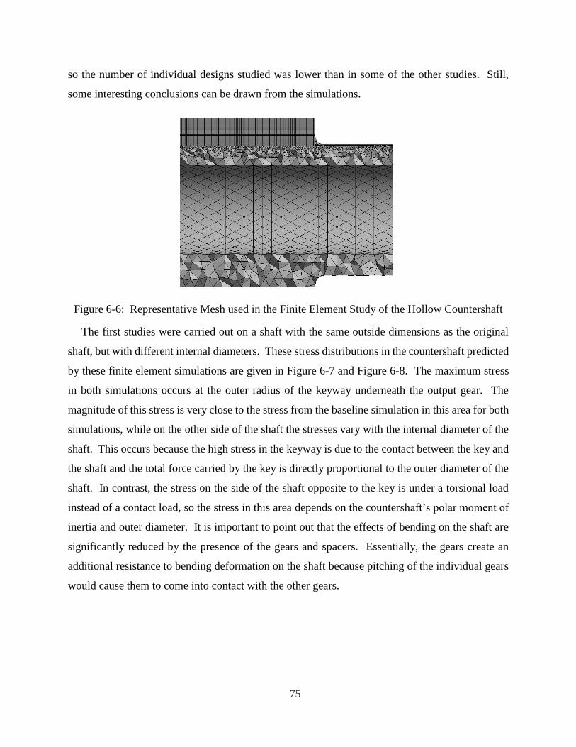
75
so the number of individual designs studied was lower than in some of the other studies. Still,
some interesting conclusions can be drawn from the simulations.
Figure 6-6: Representative Mesh used in the Finite Element Study of the Hollow Countershaft
The first studies were carried out on a shaft with the same outside dimensions as the original
shaft, but with different internal diameters. These stress distributions in the countershaft predicted
by these finite element simulations are given in Figure 6-7 and Figure 6-8. The maximum stress
in both simulations occurs at the outer radius of the keyway underneath the output gear. The
magnitude of this stress is very close to the stress from the baseline simulation in this area for both
simulations, while on the other side of the shaft the stresses vary with the internal diameter of the
shaft. This occurs because the high stress in the keyway is due to the contact between the key and
the shaft and the total force carried by the key is directly proportional to the outer diameter of the
shaft. In contrast, the stress on the side of the shaft opposite to the key is under a torsional load
instead of a contact load, so the stress in this area depends on the countershaft’s polar moment of
inertia and outer diameter. It is important to point out that the effects of bending on the shaft are
significantly reduced by the presence of the gears and spacers. Essentially, the gears create an
additional resistance to bending deformation on the shaft because pitching of the individual gears
would cause them to come into contact with the other gears.

76
Figure 6-7: Stress Distribution in a Hollow Countershaft with and Outer Diameter of 44.1mm
[1.735 in] and an internal Diameter of 6.35 mm [0.25 in]
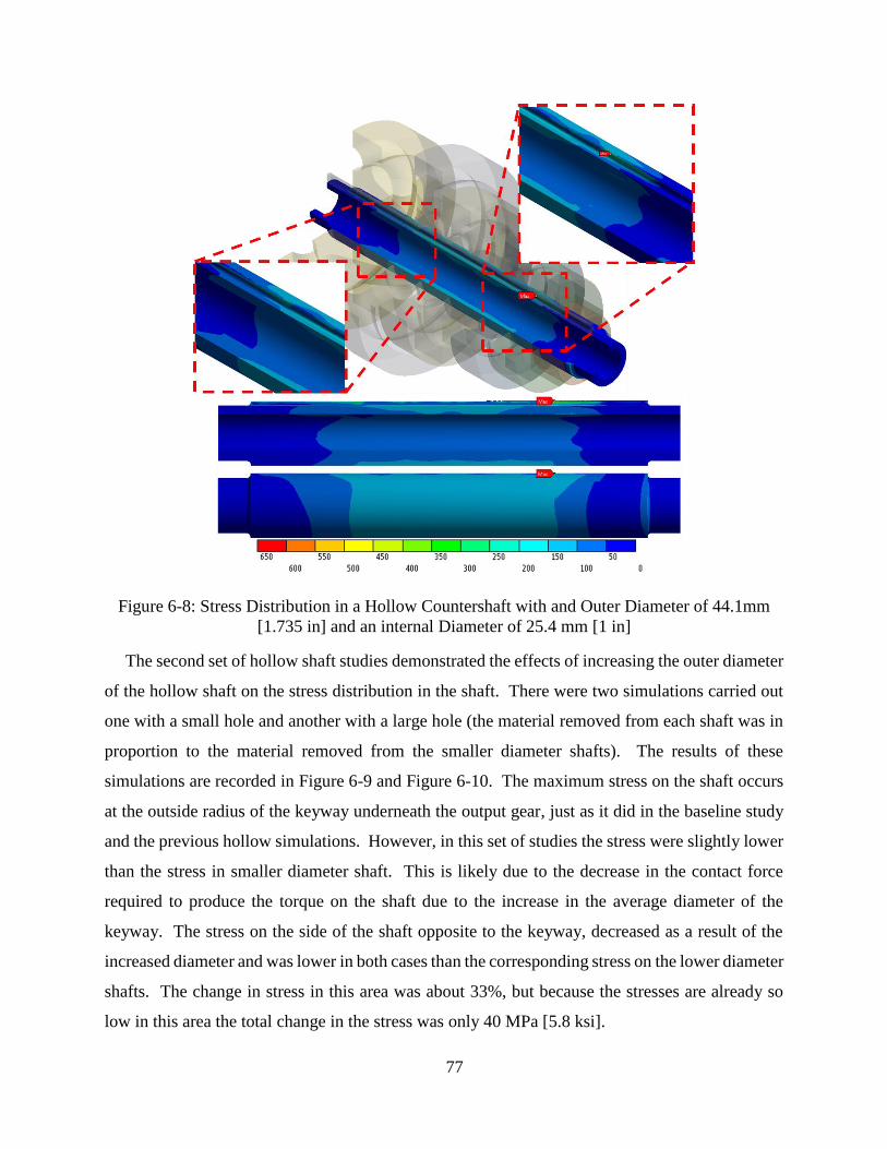
77
Figure 6-8: Stress Distribution in a Hollow Countershaft with and Outer Diameter of 44.1mm
[1.735 in] and an internal Diameter of 25.4 mm [1 in]
The second set of hollow shaft studies demonstrated the effects of increasing the outer diameter
of the hollow shaft on the stress distribution in the shaft. There were two simulations carried out
one with a small hole and another with a large hole (the material removed from each shaft was in
proportion to the material removed from the smaller diameter shafts). The results of these
simulations are recorded in Figure 6-9 and Figure 6-10. The maximum stress on the shaft occurs
at the outside radius of the keyway underneath the output gear, just as it did in the baseline study
and the previous hollow simulations. However, in this set of studies the stress were slightly lower
than the stress in smaller diameter shaft. This is likely due to the decrease in the contact force
required to produce the torque on the shaft due to the increase in the average diameter of the
keyway. The stress on the side of the shaft opposite to the keyway, decreased as a result of the
increased diameter and was lower in both cases than the corresponding stress on the lower diameter
shafts. The change in stress in this area was about 33%, but because the stresses are already so
low in this area the total change in the stress was only 40 MPa [5.8 ksi].

78
Figure 6-9: Stress Distribution in a Hollow Countershaft with and Outer Diameter of 50.8 mm
[2 in] and an internal Diameter of 7.32 mm [0.288 in]
Figure 6-10: Stress Distribution in a Hollow Countershaft with and Outer Diameter of 50.8 mm
[2 in] and an internal Diameter of 29.3 mm [1.153 in]

79
A few more simulations were carried out on the hollow countershaft with even more material
removed from the shaft so that trends in the changes in the stresses could be better examined. The
numerical results of these simulations are plotted in addition to the results of the four simulations
examined previously in this section in Figure 6-11 through Figure 6-13. One can see a very tight
grouping between the maximum stress in the baseline and the 44.1 mm [1.735 in] and 50.8 mm [2
in] diameter hollow shafts. The stress on the opposite side of the keyway, however, demonstrates
a much larger spacing (percentage wise). The amount of weight which could be removed from
the shaft depends on whether one makes the decision based on the stresses on the keyway or based
on the stresses elsewhere in the shaft. If the maximum stress is the deciding factor, the weight can
only be reduced by about 0.5 kg [1.1 lbs] per shaft or 1.5 kg [3.3 lbs] total. However, if the stress
in the keyway is ignored, the weight saved could be upwards of 2 kg [4.4 lbs] per shaft or 6 kg
[13.2 lbs] total. The major source of stress on the countershaft in this particular gearbox is the
keyway. Using a lower stress alternative to the keyway, like a splined shaft or directly machining
the gears onto flanges in the shaft, would allow the designer to take full advantage of the material’s
strength to greatly reduce the shaft’s weight.
Figure 6-11: Maximum Stress in the Countershaft as a Function of the Wall Thickness to Outer
Diameter Ratio
0
100
200
300
400
500
600
700
800
0 0.1 0.2 0.3 0.4 0.5
Stre
ss [
MPa
]
Wall Thickness/Diameter
OD 1.735 in [44.069 mm]OD 2 in [50.8 mm]Baseline [MPa]

80
Figure 6-12: Stress on Opposite Side of Keyway in the Hollow Countershaft as a Function of the
Wall Thickness to Outer Diameter Ratio
Figure 6-13: Mass of the Countershaft as Function of Wall Thickness to Outer Diameter Ratio
6.4 Bimetallic Countershaft
In this section the simulations are focused on bimetallic counter shafts. Instead of removing
the material from the inside it will be replaced with material which has a much lower density. This
may allow for the weight reduction of complicated parts that are difficult to forge in a hollow
configuration. The geometry used in these simulations is identical to the geometry used in the
0
20
40
60
80
100
120
140
160
0 0.1 0.2 0.3 0.4 0.5
Stre
ss o
n O
pp
osi
te S
ide
of
Keyw
ay
[MPa
]
Wall Thickness/Diameter
OD 1.735 in [44.069 mm]
OD 2 in [50.8 mm]
Baseline [MPa]
0
0.5
1
1.5
2
2.5
3
3.5
4
4.5
5
0 0.1 0.2 0.3 0.4 0.5
Mas
s [k
g]
Wall Thickness/Diameter
OD 1.735 in [44.069 mm]
OD 2 in [50.8 mm]
Baseline [kg]
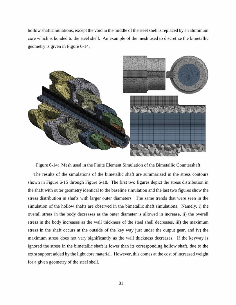
81
hollow shaft simulations, except the void in the middle of the steel shell is replaced by an aluminum
core which is bonded to the steel shell. An example of the mesh used to discretize the bimetallic
geometry is given in Figure 6-14.
Figure 6-14: Mesh used in the Finite Element Simulation of the Bimetallic Countershaft
The results of the simulations of the bimetallic shaft are summarized in the stress contours
shown in Figure 6-15 through Figure 6-18. The first two figures depict the stress distribution in
the shaft with outer geometry identical to the baseline simulation and the last two figures show the
stress distribution in shafts with larger outer diameters. The same trends that were seen in the
simulation of the hollow shafts are observed in the bimetallic shaft simulations. Namely, i) the
overall stress in the body decreases as the outer diameter is allowed in increase, ii) the overall
stress in the body increases as the wall thickness of the steel shell decreases, iii) the maximum
stress in the shaft occurs at the outside of the key way just under the output gear, and iv) the
maximum stress does not vary significantly as the wall thickness decreases. If the keyway is
ignored the stress in the bimetallic shaft is lower than its corresponding hollow shaft, due to the
extra support added by the light core material. However, this comes at the cost of increased weight
for a given geometry of the steel shell.

82
Figure 6-15: Stress Distribution in a Bimetallic Countershaft with and Outer Diameter of
44.1mm [1.735 in] and an internal Diameter of 6.35 mm [0.25 in]
Figure 6-16: Stress Distribution in a Bimetallic Countershaft with and Outer Diameter of
44.1mm [1.735 in] and an internal Diameter of 25.4 mm [1 in]

83
Figure 6-17: Stress Distribution in a Bimetallic Countershaft with and Outer Diameter of 50.8
mm [2 in] and an internal Diameter of 7.32 mm [0.288 in]
Figure 6-18: Stress Distribution in a Bimetallic Countershaft with and Outer Diameter of 50.8
mm [2 in] and an internal Diameter of 29.3 mm [1.153 in]

84
A few additional simulations were run on the bimetallic counter shafts to better determine the
trends in the stress and weight of the component. The numerical results are plotted with the
numerical results from the simulations which were previously discussed in this section. Figure
6-19 illustrates how the maximum stress in the counter shaft varies as the ratio of the steel wall
thickness to the outer diameter of the shaft changes. The trend in these simulations is less clear
than it is in the simulations of the other parts in this study, but there appears to be a slight increase
in the stress as the wall thickness in the steel shell decreases. The stress on the opposite side of
the keyway is plotted against the steel wall thickness to outer diameter ratio in Figure 6-20. The
trend in this plot is much clearer and follow a similar path as the other parts simulated in this study.
However, it is clear that the material is not being loaded to anywhere near yield strength of typical
automotive steel grades, which means that it is not being fully utilized. Based on Figure 6-21 the
weight which can be saved by switching from a solid shaft to a bimetallic shaft is about 0.5 kg [1.1
lbs] per shaft, or 1.5 kg [3.3 lbs] total, if the stress at the keyway is made to match the baseline
simulations. If the magnitude of the stress concentration is reduced by replacing the key with a
lower stress joining technique a great deal more weight can be saved. A better joining technique
would allow the material to be loaded to higher stress levels, reducing the need for large shaft and
gear dimensions.
Figure 6-19: Maximum Stress in the Bimetallic Countershaft as a Function of the Wall Thickness
to Outer Diameter Ratio
0
100
200
300
400
500
600
700
0 0.1 0.2 0.3 0.4 0.5
Stre
ss [
MPa
]
Wall Thickness/Diameter
OD 1.735 in [44.069 mm]OD 2 in [50.8 mm]Baseline [MPa]
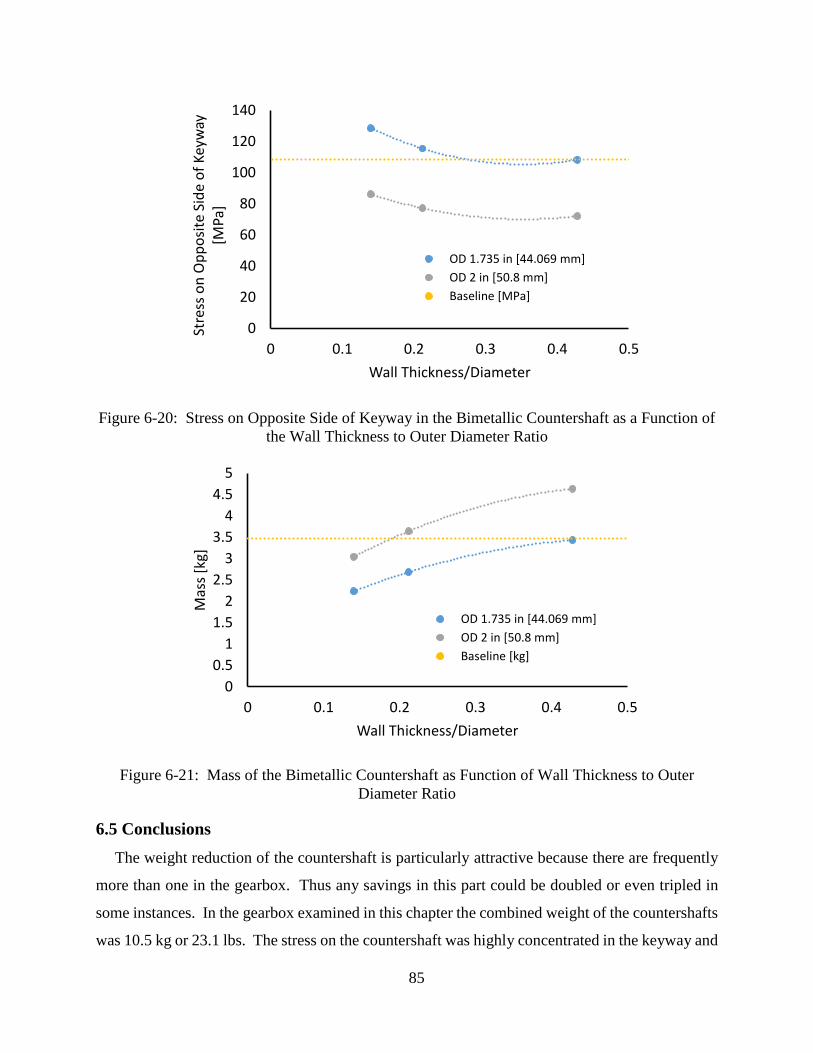
85
Figure 6-20: Stress on Opposite Side of Keyway in the Bimetallic Countershaft as a Function of
the Wall Thickness to Outer Diameter Ratio
Figure 6-21: Mass of the Bimetallic Countershaft as Function of Wall Thickness to Outer
Diameter Ratio
6.5 Conclusions
The weight reduction of the countershaft is particularly attractive because there are frequently
more than one in the gearbox. Thus any savings in this part could be doubled or even tripled in
some instances. In the gearbox examined in this chapter the combined weight of the countershafts
was 10.5 kg or 23.1 lbs. The stress on the countershaft was highly concentrated in the keyway and
0
20
40
60
80
100
120
140
0 0.1 0.2 0.3 0.4 0.5
Stre
ss o
n O
pp
osi
te S
ide
of
Keyw
ay
[MPa
]
Wall Thickness/Diameter
OD 1.735 in [44.069 mm]
OD 2 in [50.8 mm]
Baseline [MPa]
0
0.5
1
1.5
2
2.5
3
3.5
4
4.5
5
0 0.1 0.2 0.3 0.4 0.5
Mas
s [k
g]
Wall Thickness/Diameter
OD 1.735 in [44.069 mm]
OD 2 in [50.8 mm]
Baseline [kg]
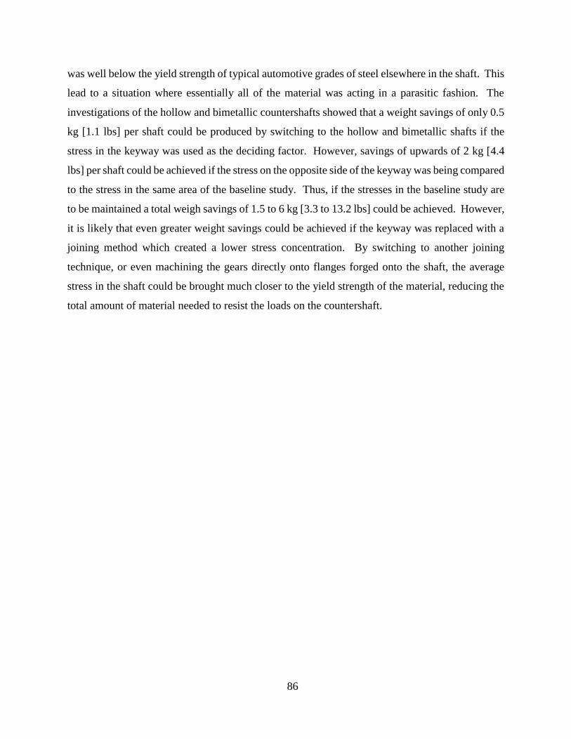
86
was well below the yield strength of typical automotive grades of steel elsewhere in the shaft. This
lead to a situation where essentially all of the material was acting in a parasitic fashion. The
investigations of the hollow and bimetallic countershafts showed that a weight savings of only 0.5
kg [1.1 lbs] per shaft could be produced by switching to the hollow and bimetallic shafts if the
stress in the keyway was used as the deciding factor. However, savings of upwards of 2 kg [4.4
lbs] per shaft could be achieved if the stress on the opposite side of the keyway was being compared
to the stress in the same area of the baseline study. Thus, if the stresses in the baseline study are
to be maintained a total weigh savings of 1.5 to 6 kg [3.3 to 13.2 lbs] could be achieved. However,
it is likely that even greater weight savings could be achieved if the keyway was replaced with a
joining method which created a lower stress concentration. By switching to another joining
technique, or even machining the gears directly onto flanges forged onto the shaft, the average
stress in the shaft could be brought much closer to the yield strength of the material, reducing the
total amount of material needed to resist the loads on the countershaft.
87
Chapter 7
Conclusions and Future Work
In the first section of the report, load maps are created that depict how the loads are transmitted
from system to system and part to part. The forces and moments which are applied to the
individual heavy duty truck components are evaluated in this section. The next section is
composed of several investigations into the weight reduction of several gearbox shafts and the axle
shafts. Two lightweight design techniques were examined: i) a hollow shaft geometry, and ii) a
bimetallic shaft configuration which utilized a low density core material.
The largest weight savings in the study were achieved by replacing the conventional, solid axle
shaft with lightweight axle shafts. The weight savings were very large because the combined
weight of the axle shafts in the heavy duty truck in much greater than the weight of the other parts
examined. Specifically, 22.5 to 29.4 kg [49.6 to 64.8 lbs] of material can be removed if the hollow
shaft design is used and 16 to 19.2 kg [35.2 to 42.2 lbs] can be removed from the vehicle if the
bimetallic variant is used. These savings are dependent on the acceptable increase in the shaft’s
diameter and feasibility of fabricating the designs.
The lightweight designs for the gear box input shaft also showed some promise, but due to the
low weight of the conventional part the actual weight removed from the vehicle is small. The
hollow input shaft design saved 1.75 kg [3.85 lbs] of weight and the bimetallic input shaft design
reduced the weight of the component by 0.9 kg [2 lbs]. It is important to note that even this small
shavings could be an important part of an aggregate weight savings created by making a series of
minor weight improvements.
The output shaft has slightly higher prospects for reducing the weight of the heavy duty truck
than the input shaft due to its larger initial weight. It was determined that a weight savings of 1.7
to 2.2 kg [3.74 to 4.84 lbs] could be achieved by switching from a solid shaft to a hollow shaft and
a savings of 1.29 kg [2.84 lbs] could be achieved if a bimetallic variant of the output shaft was
utilized. This is, of course, assuming that the lightweight designs could be fabricated and that a
slight increase in the diameter of the shaft is acceptable.
88
The countershaft examined in this report is harder to make a judgement about than the other
power train parts examined due to the high stress concentrations induced by the keyway. It was
discovered that a majority of the material in the countershaft in the reference gearbox was carrying
a stress which was much less than the yield strength of typical automotive grades of steel. The
exception to this generalization is the stress of the material in the keyway which reached very high
levels. If the stress is to be maintained at levels near the solid countershaft examined combined
weight savings of only 1.5 kg [3.3 lbs] are possible. However, if a method of joining the gears to
the shaft was adopted that had a smaller stress concentration than the keyway, it is very likely that
the size of the countershaft and gears on the shaft could be significantly reduced. This would result
in a better utilization of the strong, but heavy, steel and an overall reduced weight.
Overall, it was determined that by applying these techniques to the investigated parts that a total
weight savings of 38.4 kg [86.6 lbs] could be reached. This is, of course, subject to the feasibility
of actually fabricating the lightweight designs.
In the next phase of the project will focus on the forging techniques which will be needed to
create some of the light weight parts suggested in this report. It will help to determine the
feasibility of the designs in light of up to date forging practices and materials as well as identify
any potential problems or limitations that may arise during the development of these new heavy
duty light weight parts.

89
References
[1] "§ 20-118. Weight of Vehicles and Load." North Carolina General Statutes. North Carolina
General Assembly. Web.
<http://www.ncleg.net/EnactedLegislation/Statutes/HTML/BySection/Chapter_20/GS_20-
118.html>.
[2] Nash, Michael. "SuperTruck Highlights Potential for Further Truck Efficiency, Says DTNA."
Automotive World. 11 June 2015. Web.
<http://www.automotiveworld.com/analysis/supertruck-highlights-potential-truck-efficiency-
says-dtna/>.
[3] "Detroit Engines Brochure." Demand Detroit. Detroit Diesel Corporation, 2014. Web. 23 Mar.
2016. <https://www.demanddetroit.com/pdf/Engines/0814-Detroit_Engines_Brochure.pdf>.
[4] "Powertrain | Volvo Trucks.” Volvo Trucks, 2016. Web.
<http://www.volvotrucks.us/powertrain/>.
[5] "Cummins 2013 ISX15 For Truck Applications." On-Highway Brochures. Cummins Inc.,
2013. Web. <http://cumminsengines.com/brochure-download.aspx?brochureid=265>.
[6] Ali, Y.; Hanna, M. A.; Borg, J. E. “In-cylinder pressure characteristics of a CI engine using
blends of diesel fuel and methyl esters of beef tallow”. Trans. ASAE 1996, 39, 799- 804
[7] "Mack ES T310 ServiceManual." Global Transmission Supply. Mack Trucks, Inc., 2002. Web.
<http://globaltransmissionsupply.com/pdf/transmissions/Mack_ES_T310_Service_Manual.p
df>.
[8] "Mack Maxitorque ES 10 Speed Transmission T310m." Global Transmission Supply. Mack
Trucks, Inc., 2002. Web.
<http://www.globaltransmissionsupply.com/pdf/transmissions/mack-maxitorque-es-10-
speed-transmission-t310m.pdf>.
[9] "Driveline Specifications for the New Volvo FMX." Volvo Trucks Egypt. Volvo Trucks, 2011.
Web. <http://www.volvotrucks.com/trucks/egypt-market/en-eg/trucks/volvo-fmx-euro-
3/Specifications/Pages/driveline.aspx>.