Weierstraß-Institutfür Angewandte Analysis und StochastikLeibniz-Institut im Forschungsverbund Berlin e. V.

Preprint ISSN 0946 – 8633

Global higher integrability of minimizers of variational

problems with mixed boundary conditions

Alice Fiaschi 1, Dorothee Knees 2, Sina Reichelt 2

submitted: November 22, 2011

1 IMATI-CNRvia Ferrata 1I-27100 PaviaItalyE-Mail: alice.fiaschi@imati.cnr.it

2 Weierstrass InstituteMohrenstr. 3910117 BerlinGermanyE-Mail: dorothee.knees@wias-berlin.de

sina.reichelt@wias-berlin.de

No. 1664

Berlin 2011

2010 Mathematics Subject Classification. 74C05, 49N60, 49S05, 35B65.

Key words and phrases. Higher integrabilty of gradients of minimizers, p-growth, mixed boundary conditions, dam-age, uniform Caccioppoli-like inequality.

This research was supported by the Deutsche Forschungsgemeinschaft via the project C35 Global higher integra-bility of minimizers of variational problems with mixed boundary conditions of the Research Center MATHEON andthe FP7-IDEAS-ERC-StG Grant 200497 BioSMA: Mathematics for Shape Memory Technologies in Biomechanics.

Edited byWeierstraß-Institut für Angewandte Analysis und Stochastik (WIAS)Leibniz-Institut im Forschungsverbund Berlin e. V.Mohrenstraße 3910117 BerlinGermany

Fax: +49 30 2044975E-Mail: preprint@wias-berlin.deWorld Wide Web: http://www.wias-berlin.de/

Abstract

We consider functionals of the type

F(u) :=

∫Ω

F (x, u,Du) dx,

where Ω ⊂ Rn is a Lipschitz domain with mixed boundary conditions such that ∂Ω =

∂DΩ ∪ ∂NΩ. The aim of this paper is to prove that, under uniform estimates within certain

classes of p-growth and coercivity assumptions on the density F , the minimizers u are of

higher integrability order, meaning u ∈ W 1,p+ε(Ω;RN ) for a uniform ε > 0. The results are

applied to a model describing damage evolution in a nonlinear elastic body and to a model

for shape memory alloys.

1 Introduction

This paper investigates integrability properties for vector-valued minimizers of integral function-

als on nonsmooth domains with densities having p-growth and with mixed boundary conditions.

The natural regularity for minimizers of such functionals is W 1,p-regularity.

However, in many applications further regularity properties for minimizers, or for solutions

to PDEs are desirable. It is well-known that, in the case of solutions to PDEs, higher regularity

properties of solutions allow, for instance, to predict convergence rates of numerical schemes for

PDEs, or to derive first order necessary conditions in optimal control problems. Analogously, for

minimizers of functionals of the type we are considering, it is fundamental in many applications

to obtain higher integrability. In particular, higher integrability properties of minimizers are

important in the discussion of elasticity problems which are coupled with further phenomena

like phase separation or damage processes, and where the elasticity coefficients depend on the

phase field or damage variables.

Since in typical applications the domain representing the model reference configuration has a

nonsmooth boundary with corners and edges and since different types of boundary conditions

may be imposed on different parts of the boundary, regularity results are needed that take into

account all these peculiarities. We also highlight that in the applications to elasticity models

with state-dependent coefficients, it is of great interest to study the robustness of the higher

integrability properties with respect to classes of coefficients satisfying uniform bounds. Uniform

bounds are required as well in general time-dependent models, in homogenization problems and

in general problems where a further passage to the limit has to be performed.

The paper focuses on minimizers of integral functionals of the type

F(u) =

∫ΩF (x, u,Du) dx, (1.1)

where u : Ω → RN is a vector-valued function and Ω is the n-dimensional physical domain.

The energy density F shall have p-growth and satisfy a suitable coercivity estimate. Convexity

or differentiability of F in Du are not required. As main result, we derive the global higher

1

integrability of minimizers and their gradients on nonsmooth domains, with mixed boundary

conditions and with nonsmooth coefficients, i.e. we show that there exists q > p such that the

minimizers belong to W 1,q(Ω). Moreover, we provide results and estimates, which are uniform

within certain classes of functionals.

We are aware that the higher integrability result itself is not “surprising”. However, for

systems with mixed boundary conditions on nonsmooth domains, no results are available in the

literature, as we point out here below.

The investigation of higher integrability of solutions to elliptic PDEs and of minimizers of

integral functionals has a long tradition. For scalar linear elliptic equations (i.e. p = 2) of

second order with L∞-coefficients and mixed boundary conditions a general integrability result

was proved in [Gro89], stating that there exists a q > 2 such that the differential operator is an

isomorphism between the Sobolev spaces W 1,qD (Ω) =

u ∈ W 1,q(Ω)

∣∣u|∂DΩ = 0

and W−1,q(Ω)

with suitable boundary conditions. This result was extended in [HMW11] to the system of linear

elasticity and a closely related strongly monotone system for nonlinear elasticity (p = 2). The

arguments used are localization principles, fixed point and reflection arguments and rely on a

generalized Garding inequality for the Laplace operator [Sim72].

A different approach was followed by Giaquinta and Giusti [GG82, Giu03] who in a first

step showed, for the vector-valued case and general p, that minimizers of integral-functionals

satisfy a Caccioppoli inequality which is a reverse Holder inequality on increasing domains.

Subsequently, a generalized Gehring-type lemma due to Giaquinta and Modica [GM79] allows

to conclude the higher integrability of minimizers meaning that there exists q > p such that

minimizers belong toW 1,q(Ω). The results are proved for nonsmooth domains with pure Dirichlet

boundary conditions for quite general functionals satisfying suitable upper p-growth estimates

and a coercivity estimate. In [NW91] these arguments were extended to nonlinear elliptic systems

of second order with mixed boundary conditions, with the Sobolev space W 1,2(Ω) as the basic

space (i.e. p = 2). In [SW94], the elasticity system is studied on smooth domains with similar

techniques. Further, refined estimates for smooth domains under strong convexity assumptions

on the energy density can be found in [KM06]. To our knowledge, for the general vector-valued

case with energy densities of general p-growth (p 6= 2) on nonsmooth domains with mixed

boundary conditions no global integrability results are available in the literature.

In the proof of our main result, we follow the general lines of Naumann-Wolff’s proof of higher

integrability for systems of elliptic PDEs ([NW91]). More precisely, we use the localization

techniques introduced in [Gro89] and we are interested in deriving Caccioppoli-like estimates

for model problems on cubes with mixed boundary conditions. However, we do not deal with

PDEs, but with minimizers of possibly non-differentiable functionals with general p-growth and

more general coercivity assumptions, allowing to treat also elasticity models with symmetric

gradients. For these reasons, the proof of the Caccioppoli-type inequality in our case is more

delicate, compared to [NW91], and we need to adapt the tools presented in [Giu03] to the

situation with mixed boundary condition. In view of the applications we have in mind, special

2

attention is devoted to the uniformity of our estimates.

In the last part of the paper, we apply our Main Theorem 3.1 to time-dependent elastic models

with internal parameters. In particular, we prove the higher integrability of the displacement

field of a rate-independent damage model. This model is based on a quasi-convex elastic energy,

a multiplicative coupling between the damage variable and the elastic fields and an inequality

constraint on the damage variable preventing self-healing. We also use the higher integrability

result to generalize the boundary condition considered in the models analyzed in [Fia10, FKS11]

for phase transitions and damage evolution, respectively. The evolution considered there is writ-

ten in terms of Young measures and to prove the stability condition, in particular, continuity

properties along suitable sequences of minimizers are needed. This continuity is actually ob-

tained thanks to the uniform higher integrability of the solutions to the discrete minimization

problem. With similar arguments, the uniform global higher integrability finally is derived for

the displacements and the internal variables of so-called stable states, cf. [FM06], occurring in

the energetic formulation of rate-independent processes, see Section 4.5.

2 Setting of the problem and assumptions

Let Cr(y) = y + (−r, r)n ⊂ Rn be the open cube with side length 2r centered in y.

Definition 2.1 (Regular domain [Gro89]). A set G ⊂ Rn is called regular, if G is a bounded

domain and if for every x0 ∈ ∂G there exist subsets Ux0 ⊂ Rn and a bi-Lipschitz transformation

Tx0 : Ux0 → C1(0) such that Ux0 is an open neighborhood of x0 ∈ Rn and Tx0(Ux0) = C1(0).

Furthermore, Tx0(x0) = 0 and the image Tx0(Ux0 ∩G) is one of the following sets:

E1 := y ∈ Rn | |y|∞ < 1, yn > 0,E2 := y ∈ Rn | |y|∞ < 1, yn ≥ 0,E3 := y ∈ E2 | yn > 0 or y1 > 0.

Here, | · |∞ denotes the supremum norm so that Ei, i = 1, 2, 3, are n-dimensional cuboids.

On regular domains in the sense of Definition 2.1, the Sobolev embedding theorems and there-

fore Poincare type inequalities are valid, e.g. see Theorems 3.11, 3.12 and 3.13 in [Giu03]. In

the proofs of the underlying Theorems 3.6 and 3.10 in [Giu03], one can easily check that the

assumptions on the boundary therein are not more restrictive than in Definition 2.1. We set

Ω =G, ∂NΩ =

(G\Ω) for the Neumann boundary and

∂DΩ = ∂Ω\∂NΩ for the Dirichlet boundary.(2.1)

Definition 2.2 (Admissible test function [Gro89]). For p ∈ (1,∞), we call ϕ an admissible test

function on Ω, if ϕ ∈W 1,pD (Ω;RN ) with

W 1,pD (Ω;RN ) :=

ϕ ∈W 1,p(Ω;RN )

∣∣ϕ|∂DΩ = 0.

3

The functional F : W 1,pD (Ω;RN ) → R that will be subject to our upcoming investigations is

defined as

F(u) :=

∫ΩF (x, u,Du) dx,

with a density F : Ω× RN × Rn×N → R, which will be specified later. The following definition

of Q-minimizers is in the spirit of quasi-minimizers as in Definition 6.1 in [Giu03].

Definition 2.3 (Q-minimizer). We call u ∈W 1,pD (Ω;RN ) a Q-minimizer of F for some Q ≥ 1,

if for all compact sets K ⊂ Rn and all ϕ ∈W 1,pD (Ω;RN ) such that ϕ|Ω\K = 0 there holds∫

Ω∩KF (x, u,Du) dx ≤ Q

∫Ω∩K

F (x, u+ ϕ,D(u+ ϕ)) dx.

Obviously, every global minimizer of F with respect to W 1,pD (Ω;RN ) is a Q-minimizer with

Q = 1. Throughout the paper the following assumptions should hold true.

Assumption on the domain Ω:

(A1) The set G ⊂ Rn, n ≥ 2 is regular as in Definition 2.1 and Ω, ∂DΩ, ∂NΩ are given as in

(2.1). Note that ∂DΩ or ∂NΩ may possibly be empty.

Assumptions on the integrand F :

(A2) The volume density F : Ω × RN × Rn×N → R is a Caratheodory function satisfying for

p ∈ (1,∞), c0 > 0 and almost all x ∈ Ω and all u ∈ RN , A ∈ Rn×N the upper estimate

|F (x, u,A)| ≤ c0 (|A|+ ϑ(x, u))p ,

where ϑ(x, u)p = b1(x)|u|γ + b2(x) for some

γ ∈

(0, p∗) with p∗ = pnn−p , if p < n,

(0,∞), if p ≥ n.(2.2)

Here, the functions b1 and b2 satisfy b2 ∈ L1(Ω) and b1 ∈ Lσ(Ω) with b1, b2 ≥ 0 and

σ =

p∗

p∗−γ , if p < n,

1 + δ, if p = n,

1, if p > n,

(2.3)

for some arbitrary δ > 0.

We define for p ≤ n:

p∗ :=

pnn−p , if p < n,γ(1+δ)

δ , if p = n,(2.4)

with γ, δ as in (A2). Observe that W 1,p(Ω) is continuously embedded in Lp∗(Ω) for p ≤ n and

for p > n, we find W 1,p(Ω) ⊂ L∞(Ω).

4

(A3) There exists a function F : Rn×N → R such that

(a) F (0) = 0,

(b) there exist constants ν > 0, c1 ≥ 0 such that for every ϕ ∈W 1,pD (Ω;RN ) there holds∫

ΩF (Dϕ) dx ≥ ν‖Dϕ‖pLp(Ω) − c1‖ϕ‖pLp(Ω),

(c) for almost all x ∈ Ω and all u ∈ RN , z ∈ Rn×N the lower estimate

F (x, u,A) ≥ F (A)− ϑ(x, u)p

is valid.

Remark 2.1. According to Theorem 4.3.1 in [Zie89], an element ` of the dual space

W 1,pD (Ω;RN )∗ can be represented by a pair (H0, H1) ∈ Lp′(Ω;RN )× Lp′(Ω;Rn×N ) with

1p + 1

p′ = 1 such that

〈`, u〉 =

∫ΩH0 · u+H1 : ∇u dx for all u ∈W 1,p

D (Ω;RN ).

Here, A : B = tr (ATB) for A,B ∈ Rn×N . If the assumptions (A2)-(A3) hold true for a function

F : Ω× RN × Rn×N → R, then for every (H0, H1), the function

F (x, u,A) := F (x, u,A)−H0 · u−H1 : A

satisfies (A2)-(A3), too, with γ, b1, b2 and˜F as given below:

Case γ ∈ (0, 1) : γ = 1, σ =

p∗

p∗−1 , if p < n,

1 + δ for some δ > 0, if p = n,

1, if p > n,

c0 = c(c0, p, γ) and ϑ(x, u)p = b1|u|γ + b2 with

b1 = b(1−σ(1−γ))γ−1

1 + |H0| ∈ Lσ(Ω), b2 = b2 + bσ1 + |H1|p′ ∈ L1(Ω).

Case γ ∈ [1, p∗) : γ = γ, σ = σ

c0 = c(c0, p, γ) and ϑ(x, u)p = b1|u|γ + b2 with

b1 = b1 + |H0|p−γp−1 ∈ Lσ(Ω), b2 = b2 + |H0|p

′+ |H1|p

′ ∈ L1(Ω).

In any case:˜F (A) = F (A)− ν

2 |A|p, ν = ν2 and c1 = c1.

For the sake of Remark 2.1, we can absorb linear functionals of the type u 7→ 〈`, u〉 into the

density F .

5

Definition 2.4. For a set G ⊂ Rn satisfying (A1) and a set of parameters and functions

(p, ν, c0, c1, b1, b2, γ) with p ∈ (1,∞), ν, c0 > 0, c1 ≥ 0, b1 ∈ Lσ(Ω), b2 ∈ L1(Ω) with σ and γ as

in (2.3) and (2.2), respectively, we introduce the class of functionals

F(Ω, p, ν, c0, c1, b1, b2, γ) :=

functionals F(u) =

∫ΩF (x, u,Du) dx with densities F fulfilling

assumptions (A2)-(A3) with the set of parameters and functions (p, ν, c0, c1, b1, b2, γ).

3 Main Theorem and proof

The main result of this paper is the following theorem, which states the uniform higher integra-

bility for the gradient Du of Q-minimizers u.

Theorem 3.1 (Main Theorem). Assume (A1) holds true and let the set of parameters and

functions (p, ν, c0, c1, b1, b2, γ) be chosen according to Definition 2.4. Further, let Q ≥ 1, p∗ as

in (2.4), σ as in (2.3) and assume that,

there exists t > 1 such that bσ1 , b2 ∈ Lt(Ω). (3.1)

Let further Cb ≥ 0. Then there exist constants c > 0 and q > 1 such that for all

F ∈ F(Ω, p, ν, c0, c1, b1, b2, γ) and all Q-minimizers u ∈W 1,pD (Ω;RN ) of F satisfying

‖u‖W 1,p(Ω) ≤ Cb, (3.2)

it holds: Du ∈ Lpq(Ω;Rn×N ). Moreover, if p ≤ n there holds∫Ω

(|Du|p + |u|p∗

)qdx ≤ c

(∫Ω|Du|p + |u|p∗ dx

)q+

∫Ω

(bσ1 + b2 + 1)q dx

, (3.3)

and if p > n ∫Ω|Du|pq dx ≤ c

(∫Ω|Du|p dx

)q+

∫Ω

(bσ1 + b2 + 1)q dx

. (3.4)

Remark 3.1. In consideration of the upcoming Remarks 3.3 and A.1 in the Appendix, the

constants c and q in Theorem 3.1 only depend on the parameters Q, p, ν, c0, c1, γ, Cb and the full

norm ‖bσ1 + b2‖L1(Ω), but not on local properties of b1 and b2.

The Main Theorem provides uniform higher integrability estimates for all minimizers of func-

tionals belonging to certain classes F(Ω, p, ν, c0, c1, b1, b2, γ) and admitting the same upper bound

Cb. A sufficient condition leading to such uniform bounds is formulated in Lemma 3.1, here be-

low.

Lemma 3.1. Assume that Ω satisfies assumption (A1) and λn−1(∂DΩ) > 0. Let the set of

parameters and functions (p, ν, c0, c1, b1, b2, γ) be chosen as in Definition 2.4 with γ < p and

6

c1 = 0. Let further Q ≥ 1. Then there exists a constant c > 0 such that for all F from

F(Ω, p, ν, c0, c1, b1, b2, γ) and all Q-minimizers u ∈W 1,pD (Ω;RN ) of F , we have

‖u‖pW 1,p(Ω)

≤ c(‖b1‖αLσ(Ω) + ‖b2‖L1(Ω)

),

where α = pp−γ ∈ (1,∞) and c only depend on the parameters p, ν, c0, γ and Q.

Proof. Let u ∈ W 1,pD (Ω;RN ) be a Q-minimizer of F for an arbitrary F belonging to

F(Ω, p, ν, c0, c1, b1, b2, γ). By choosing ϕ = −u and K such that Ω ∩ K = Ω in Definition

2.3, we find

F(u) ≤ QF(0) ≤ Q∫

Ωc0ϑ(x, 0)p dx = Qc(c0)‖b2‖L1(Ω). (3.5)

Now we derive a lower estimate for F(u) by exploiting the assumption (A3) with c1 = 0:

F(u) ≥∫

ΩF (Du)− ϑ(x, u)p dx ≥ ν‖Du‖pLp(Ω) −

∫Ωb1|u|γ + b2 dx. (3.6)

Combining (3.5)-(3.6), one obtains

ν‖Du‖pLp(Ω) ≤ c(Q, c0)‖b2‖L1(Ω) +

∫Ωb1|u|γ dx. (3.7)

In the case p ≤ n, applying Holder’s inequality with σ and σ′ = p∗

γ and taking into account the

embedding W 1,p(Ω) ⊂ Lp∗(Ω) in combination with the Poincare inequality gives

ν‖Du‖pLp(Ω) ≤ c(Q, p, c0)(‖b2‖L1(Ω) + ‖b1‖Lσ(Ω)‖Du‖γLp(Ω)

). (3.8)

In the case p > n, similar considerations based on the embedding W 1,p(Ω) ⊂ L∞(Ω) yield (3.8),

as well. We apply Young’s inequality to the second term on the right-hand side in (3.8) with

α = pp−γ ∈ (1,∞) and α′ = p

γ so that we obtain for every ε > 0

ν‖Du‖pLp(Ω) ≤ c(Q, p, c0)(‖b2‖L1(Ω) + C(ε)‖b1‖αLσ(Ω) + ε‖Du‖pLp(Ω)

). (3.9)

If we now choose ε < ν2c , we obtain by the classical Poincare inequality

‖u‖pW 1,p(Ω)

≤ 2c(Q, p, ν, c0, γ)(‖b2‖L1(Ω) + ‖b1‖αLσ(Ω)

).

The proof of the Main Theorem 3.1 will now be given in several steps and follows the structure

of [NW91]:

1. Transformation of the open sets Ux0 ⊂ Rn onto cubes C1(0) with a one-to-one Lipschitz

mapping Tx0 .

2. Proof of a Caccioppoli-type inequality in the spirit of Theorem 6.5 in [Giu03] for a model

problem on the half cube E3 (Lemmata 3.2 and 3.3).

7

3. Extension of the estimates from half cubes to full cubes by reflection (Corollary 3.1).

4. Deriving from Caccioppoli’s inequality the higher integrability of the gradient Du by ap-

plying a result from Giaquinta and Modica (Theorem A.3), which is based on Gehring’s

lemma.

3.1 The Transformation T

We recall that C1(0) is the unit cube with side length 2 centered in 0 and C+1 (0) is its upper half.

For x0 ∈ ∂Ω, let Tx0 be the bi-Lipschitz transformation Tx0 : Ux0 ∩Ω→ C+1 (0) with Tx0(x) = y,

existing after (A1). Since the domain Ω is compact, there exists an open covering of Ω of the

form

Ω ⊂ Ω0 ∪N⋃i=1

T−1x0i

(C18(0)), (3.10)

for a finite number of x0i ∈ ∂Ω and some set Ω0 ⊂⊂ Ω. In the following, we focus on the

boundary sets Ux0 . The higher integrability result for Ω0 can be found in Definition 6.3 and

Theorem 6.7 in [Giu03]. Further, there exist 0 < λ0 ≤ λ∗ <∞ such that for

λi(y) := |det DT−1x0i

(y)|

we have λi ∈ L∞(C1(0)) with λ0 ≤ λi(y) ≤ λ∗ almost everywhere. For x0 ∈ x0i Ni=1 fixed, we

set

v := u T−1x0

and F (y, v, A) := F (T−1x0

(y), v, ADTx0 |T−1

x0(y))λi(y). (3.11)

In the following, we suppress the dependency of the transformation Tx0 on x0. The transforma-

tion formula yields for T−1(C+1 (0)) = Ux0 ∩ Ω:∫

Ux0∩ΩF (x, u(x),Dxu(x)) dx

=

∫C+

1 (0)F (T−1(y), u(T−1(y)),Dxu(T−1(y))DT |T−1(y))|det DT−1(y)| dy

=

∫C+

1 (0)F (y, v(y),Dyv(y)) dy.

Next we show that there exist constants and functions ν, c0, c1, b1, b2 with ν, c0 > 0, c1 ≥ 0,

b1 ∈ Lσ(C+1 (0)), b2 ∈ L1(C+

1 (0)) such that for all F ∈ F(Ω, p, ν, c0, c1, b1, b2, γ) and all x0 ∈x0

i Ni=1 it holds

F(w) :=

∫C+

1 (0)F (y, w,Dw) dy ∈ F(C+

1 , p, ν, c0, c1, b1, b2, γ).

Indeed, let us set

˜F (y,A) := F (ADT |T−1(y))λi(y) and ϑ(y, w) := ϑ(T−1(y), w)λi(y)

1p .

Then it obviously holds for almost all y ∈ C+1 (0) and all v ∈ RN , A ∈ Rn×N that

8

(A2∗) |F (y, w,A)| ≤ c(p, c0, λ∗, ρ∗)

(|A|+ ϑ(y, w)

)p, where ρ∗ = max

x0

1, ε

p2 | ε is the biggest

eigenvalue of the matrix (DTx0)T (DTx0)

,

(A3∗) F (y, w,A) ≥ ˜F (y,A)− ϑ(y, w)p. Moreover, given a function ψ ∈W 1,p(C+1 (0);RN ) with

ψ|∂C+1 (0)\(Ei∩yn=0) = 0, (3.12)

where Ei = T (Ux0 ∩ G), there holds for ϕ(x) := ψ(T (x)) with the extension ϕ = 0 on

Ω\Ux0 :∫C+

1 (0)

˜F (y,Dyψ) dy =

∫Ux0∩Ω

F (Dxϕ(x)) dx

=

∫ΩF (Dxϕ(x)) dx (since F (0) = 0)

≥(A3)

ν

∫Ux0

|Dxϕ(x)|p dx− c1

∫Ux0

|ϕ(x)|p dx

= ν

∫C+

1 (0)

∣∣Dψ(y)DT |x=T−1(y)

∣∣p| det DT−1(y)|dy

−c1

∫C+

1 (0)|ψ(y)|p|det DT−1(y)|dy

≥ νλ0ρ0

∫C+

1 (0)|Dψ(y)|p dy − c1λ

∗∫C+

1 (0)|ψ(y)|p dy,

where ρ0 = minx0

εp2 | ε is the smallest eigenvalue of the matrix (DTx0)T (DTx0)

.

Remark 3.2. Let u ∈ W 1,pD (Ω;RN ) be a Q-minimizer of F . Then v = (u|Ux0∩Ω) T−1 ∈

W 1,p(C+1 (0);RN ) is a Q-minimizer of the functional F with

F(w) :=

∫C+

1 (0)F (y, w,Dw) dy

with F as in (3.11), in the following sense: For every compact set K ⊂ Rn and every ψ ∈W 1,p(C+

1 (0);RN ) satisfying (3.12) and with ψC+1 (0)\K = 0 it holds∫

C+1 (0)∩K

F (y, v,Dv) dy ≤ Q∫C+

1 (0)∩KF (y, v + ψ,D(v + ψ)) dy.

Indeed, let ψ ∈ W 1,p(C+1 (0);RN ) satisfy (3.12) and ψ|C+

1 (0)\K = 0. Then the function ϕ : Ω →RN defined by

ϕ(x) :=

ψ(T (x)), if x ∈ T−1(C+

1 (0)),

0, if x ∈ Ω\T−1(C+1 (0)),

9

is an admissible test function for F in W 1,pD (Ω;RN ) with ϕ|

Ω\T−1(C+1 (0)∩K)

= 0 and since u is a

Q-minimizer, it follows that∫C+

1 (0)∩KF (y, v,Dv) dy =

∫T−1(C+

1 (0)∩K)F (x, u,Du) dx

≤ Q∫T−1(C+

1 (0)∩K)F (x, u+ ϕ,D(u+ ϕ)) dx = Q

∫C+

1 (0)∩KF (y, v + ψ,D(v + ψ)) dy.

From now on, we denote F with f for shortness.

3.2 A Caccioppoli-type inequality on E3

Depending on the choice of x0 ∈ ∂Ω, we are left with three different cases:

1. For x0 ∈ ∂DΩ, we have Tx0(Ux0 ∩G) = E1,

2. For x0 ∈ ∂NΩ, we have Tx0(Ux0 ∩G) = E2,

3. For x0 ∈ ∂DΩ ∩ ∂NΩ, we have Tx0(Ux0 ∩G) = E3,

where we concentrate on the last case. The other cases can be seen as special cases of the third

one. If x0 ∈ Ω0, see (3.10), the subsequent considerations can be adapted to this case in a

straightforward manner. We will now study a model problem on E3, defining

ΓD := y ∈ Rn | y1 < 0 and yn = 0 and ΓN := y ∈ Rn | y1 ≥ 0 and yn = 0

as the images of the Dirichlet and Neumann boundary under the transformation with Tx0 .

Further, we define the set of admissible test functions by

W 1,pad (C+

1 (0);RN ) :=ψ ∈W 1,p(C+

1 (0);RN )∣∣ψ|∂C+

1 (0)\ΓN = 0.

A Caccioppoli-type inequality will be derived for functions v ∈W 1,pΓD

(C+1 (0);RN ), where

W 1,pΓD

(C+1 (0);RN ) :=

ψ ∈W 1,p(C+

1 (0);RN )∣∣ψ|ΓD = 0

,

satisfying for some Q ≥ 1 and all compact sets K ⊂ Rn and all ψ ∈ W 1,pad (C+

1 (0);RN ) with

ψ|C+1 (0)\K = 0 the inequality∫

C+1 (0)∩K

f(y, v,Dv) dy ≤ Q∫C+

1 (0)∩Kf(y, v + ψ,D(v + ψ)) dy. (3.13)

Let us introduce further notation of open cuboids by setting

C+r (y0) := Cr(y

0) ∩ E1 and C−r (y0) := Cr(y0)\C+

r (y0).

Hence for y0 ∈ C+1/4(0) and 0 < r < 1

4 , we have C3r(y0) ⊂ C1(0). In Lemmata 3.2 and 3.3, here

below, we distinguish two cases for the test cuboid C+r (y0):

10

y1

yn

0

C+14

(0)C+r (y0)

C−r (y0) ΓNΓD

C1(0)

y0

Figure 1: Position of the cube C+r (y0) in the Case (II).

(I) The test cuboid C+r (y0) has no Dirichlet boundary: Cr(y

0) ∩ ΓD = ∅.

(II) The test cuboid C+r (y0) has a Dirichlet boundary: Cr(y

0) ∩ ΓD 6= ∅.

Lemma 3.2. Let y0 ∈ C+1/4(0) and 0 < r < 1

4 . Assume (I) and let p = pnn+p . For every Q ≥ 1

and Cb ≥ 0, there exists a constant c > 0, independent of r and y0 such that for all functions

v ∈W 1,pΓD

(C+1 (0);RN ) with ‖v‖W 1,p(C+

1 ) ≤ Cb satisfying (3.13) for some

F(w) =

∫C+

1

f(y, w,Dw) dy ∈ F(C+1 , p, ν, c0, c1, b1, b2, γ)

it holds: If p ≤ n and p∗ as in (2.4)

∫C+r2

(y0)|Dv|p + |v|p∗ dy ≤ c

1

rp

(∫C+r (y0)

(|Dv|p + |v|p∗

) pp

dy

)pp

+

∫C+r (y0)

bσ1 + b2 + 1 dy

.

(3.14)

In the case p > n it holds

∫C+r2

(y0)|Dv|p dy ≤ c

1

rp

(∫C+r (y0)

|Dv|p dy

)pp

+

∫C+r (y0)

b1 + b2 + 1 dy

. (3.15)

Remark 3.3. The constant c in Lemma 3.2 only depends on the parameters Q, p, ν, c0, c1, γ and

the uniform bound Cb. Either Cb is given or derived depending on the given data as in Lemma

3.1. In any case, Cb is independent of local properties of the given data b1 and b2 and so is c.

11

Observe that, for all p ∈ (1,∞), there holds p ≤ p and we find p∗ = p, i.e. W 1,p(Ω) ⊂ Lp(Ω).

Proof. Let y0 ∈ C+1/4(0) and 0 < r < 1

4 so that C3r(y0) ⊂ C1(0) and assume that Cr(y

0)∩ΓD =

∅. In the following we omit the variable y0 and just write Cr instead of Cr(y0) and C+

r instead

of C+r (y0). Assume v ∈ W 1,p

ΓD(C+

1 ;RN ) is a Q-minimizer satisfying (3.13) for some arbitrary

F ∈ F(C+1 , p, ν, c0, c1, b1, b2, γ). Let r

2 ≤ t < s ≤ r. Moreover, let ς ∈ C1(Rn; [0, 1]) be a cut-off

function such that

ς|Ct = 1, ς|Rn\Cs = 0 and |Dς| ≤ ωs−t , (3.16)

with ω > 0, independent of t and s. We set ψ := (v − vC)ς, where vC = −∫C+sv dy is the mean

value of v, and we observe that ψ ∈ W 1,pad (C+

1 ;RN ) is an admissible test function on C+s . The

gradient for the difference v − ψ = vC + (1− ς)(v − vC) satisfies

D(v − ψ) = (vC − v)Dς + (1− ς)Dv. (3.17)

Further, we estimate the gradient |Dv|p with Dv = Dψ on C+t by using (A3) as follows:∫

C+t

|Dv|p dy ≤∫C+s

|Dψ|p dy

≤ c(ν)

∫C+s

f(y, v,Dψ) + ϑ(y, v)p + c1|ψ|p dy

= c(ν)

∫C+s

f(y, v,Dv) + f(y, v,Dψ)− f(y, v,Dv) + ϑ(y, v)p + c1|ψ|p dy. (3.18)

The proof will now be given for the cases p ≤ n and p > n, separately. We start with the first

case following the argumentation of Theorem 6.5 in [Giu03] closely.

Case p ≤ n: We recall that from the definition of p∗ in (2.4) and the Sobolev embedding

theorems, it follows that W 1,p(C+1 ;RN ) is continuously embedded in Lp

∗(C+

1 ;RN ). Next we add

the quantity µ∫C+t|v|p∗ dy to both sides of (3.18) and choose the constant µ > 0 later on so that

we have for now∫C+t

|Dv|p + µ|v|p∗ dy ≤ c(ν)

∫C+s

f(y, v,Dv) + µ|v|p∗︸ ︷︷ ︸Step 1

+ f(y, v,Dψ)− f(y, v,Dv) + ϑ(y, v)p + c1|ψ|p︸ ︷︷ ︸Step 2

dy. (3.19)

We continue to estimate the right-hand side of (3.19) from above in three steps.

Step 1. By exploiting (3.13) with K = C+s , we obtain∫

C+s

f(y, v,Dv) dy ≤ Q∫C+s

f(y, v − ψ,D(v − ψ)) dy. (3.20)

12

Reinserting the term µ∫C+s|v|p∗dy in (3.20) yields∫

C+s

f(y, v,Dv) + µ|v|p∗ dy ≤ c(Q)

∫C+s

|f(y, v − ψ,D(v − ψ))|+ µ|v|p∗ dy

≤

(A2)c(Q, c0)

∫C+s

|D(v − ψ)|p + ϑ(y, v − ψ)p + µ|v|p∗ dy

≤

(3.17)c(Q, p, c0)

∫C+s

|(vC − v)Dς|p + |(1− ς)Dv|p + µ|v|p∗ + b1|v − ψ|γ + b2 dy

. (3.21)

By applying Young’s inequality with ε1 > 0, the estimation of the product b1|v − ψ|γ yields

(with σ > 1 and σ′ = p∗

γ )

b1|v|γ ≤ C(ε1)bσ1 + γp∗ ε

p∗

γ1 |v|p

∗. (3.22)

Introducing the triangle inequalities |v−ψ| ≤ |v− vC |+ |vC | as well as |v| ≤ |v− vC |+ |vC | and

remembering the assumptions on the cut-off function ς, inequality (3.21) takes the form∫C+s

f(y, v,Dv) + µ|v|p∗ dy ≤ c(Q, p, ν, c0, γ)

∫C+s

1

(s− t)p |v − vC |p

+ c(µ, ε1)(|v − vC |p

∗+ |vC |p

∗)

+ C(ε1)bσ1 + b2 dy +

∫C+s \C+

t

|Dv|p dy

, (3.23)

where c(µ, ε1) =(µ+ ε

p∗

γ1

). The factor γ

p∗ is absorbed by the first constant c(Q, p, ν, c0, γ). We

are now treating the difference |v − vC |p∗

by applying Lemma A.1 with a constant Ce,P > 0

independent of s so that we obtain

∫C+s

|v − vC |p∗dy ≤ Cp∗e,P

(∫C+s

|Dv|p dy

)p∗

p

= Cp∗

e,P

(∫C+s

|Dv|p dy

)p∗−pp(∫

C+s

|Dv|p dy

)≤ Cp∗e,PC

p∗−pp

b

∫C+s

|Dv|p dy, (3.24)

where Cb is the uniform bound for v assumed in Lemma 3.2. Inserting (3.24) in (3.23) and

splitting the integral∫C+s|Dv|p dy in one part with C+

s \C+t and another with C+

t , we arrive at

∫C+s

f(y, v,Dv) + µ|v|p∗ dy ≤ c(Q, p, ν, c0, γ, Cb, Ce,P )

∫C+s

1

(s− t)p |v − vC |p + c(µ, ε1)|vC |p

∗

+ C(ε1)bσ1 + b2 dy + (1 + c(µ, ε1))

∫C+s \C+

t

|Dv|p dy + c(µ, ε1)

∫C+t

|Dv|p dy

. (3.25)

13

Step 2. We return to inequality (3.19) and, using assumption (A2) and Dψ = Dv on C+t , we

continue to estimate as follows∫C+s

f(y, v,Dψ)− f(y, v,Dv) + ϑ(y, v)p + c1|ψ|p dy

=

∫C+s \C+

t

f(y, v,Dψ)− f(y, v,Dv) dy +

∫C+s

ϑ(y, v)p + c1|ψ|p dy

≤ c(c0)

∫C+s \C+

t

|Dψ|p + |Dv|p dy +

∫C+s

ϑ(y, v)p + c1|ψ|p dy

≤ c(p, c0)

∫C+s

1

(s− t)p |v − vC |p dy +

∫C+s \C+

t

|Dv|p dy +

∫C+s

ϑ(y, v)p + c1|ψ|p dy

.

(3.26)

Applying once more Young’s inequality with ε2 > 0 and p∗

p ∈ (1,∞) yields analogously to (3.22)∫C+s

|ψ|p dy ≤∫C+s

1 · |v − vC |p dy

≤ c(ε2)

∫C+s

|v − vC |p∗

dy + C(ε2)

∫C+s

1 dy, (3.27)

where c(ε2) = pp∗ ε

p∗

p2 . The first term in (3.27) can be treated analogously to (3.24). The term

including ϑ in (3.26) can now be estimated analogously to (3.22) and (3.24) so that (3.26) can

be written as∫C+s

f(y, v,Dψ)− f(y, v,Dv) + ϑ(y, v)p + c1|ψ|p dy

≤ c(Q, p, ν, c0, c1, γ, Cb)

∫C+s

1

(s− t)p |v − vC |p + c(ε2)|vC |p

∗+ C(ε1, ε2) (bσ1 + 1) + b2 dy

+ (1 + c(µ, ε1) + c(ε2))

∫C+s \C+

t

|Dv|p dy + (c(µ, ε1) + c(ε2))

∫C+t

|Dv|p dy

. (3.28)

We are now in the position to return to inequality (3.19) by combining the results (3.25) and

(3.28). Choosing µ, ε1 and ε2 such that c(Q, p, ν, c0, c1, γ, Cb)(c(µ, ε1) + c(ε2)) = 12 , we can

subtract the term 12

∫C+t|Dv|pdy from the right-hand side such that we obtain∫

C+t

|Dv|p + |v|p∗ dy ≤ c∫

C+s

1

(s− t)p |v − vC |p + bσ1 + b2 + 1 dy + |C+

s ||vC |p∗

+

∫C+s \C+

t

|Dv|p dy

, (3.29)

where c = c(Q, p, ν, c0, c1, γ, Cb, Ce,P ).

14

Step 3. To conclude (3.14) from (3.29), we aim to apply Lemma A.3. Since r2 < s ≤ r, we

estimate, by applying Holder’s inequality with p∗ pp ∈ (1,∞),

|C+s ||vC |p

∗ ≤ 2np∗ |C+

r |(−∫C+r

|v|dy)p∗

≤ 2np∗ |C+

r |(−∫C+r

|v|p∗ pp dy

)pp

≤ 2n(p∗+1) rn(r−n

)n+pn︸ ︷︷ ︸

r−p

(∫C+r

|v|p∗ pp dy

)pp

. (3.30)

Further, applying Poincare’s inequality (Lemma A.1) with p∗ = p, we find∫C+s

|v − vC |p dy ≤∫C+r

|v − vC |p dy ≤ Cpe,P(∫

C+r

|Dv|p dy

)pp. (3.31)

Enlarging the right-hand side term∫C+s \C+

t|Dv|pdy in (3.29) to

∫C+s \C+

t|Dv|p + |v|p∗dy, adding

on both sides c∫C+t|Dv|p + |v|p∗dy and then dividing by c+ 1, yields with (3.30) and (3.31)

∫C+t

|Dv|p + |v|p∗ dy ≤ c

c+ 1

1

(s− t)p(∫

C+r

|Dv|p dy

)pp

+1

rp

(∫C+r

|v|p∗ pp dy

)pp

+

∫C+r

bσ1 + b2 + 1 dy

+

c

c+ 1

∫C+s

|Dv|p + |v|p∗ dy. (3.32)

Finally, observing 0 < cc+1 < 1 and setting β := 1 < p, Z(t) :=

∫C+t|Dv|p + |v|p∗ dy as well as

A :=

(∫C+r

|Dv|p dy

)pp, B := 0 and C :=

1

rp

(∫C+r

|v|p∗ pp dy

)pp

+

∫C+r

bσ1 + b2 + 1 dy,

we find using Lemma A.3 that

∫C+r2

|Dv|p + |v|p∗ dy ≤ c

1

rp

(∫C+r

|Dv|p dy

)pp

+1

rp

(∫C+r

|v|p∗ pp dy

)pp

+

∫C+r

bσ1 + b2 + 1 dy

.

(3.33)

From (3.33) follows (3.14) directly, where the constant c only depends on the parameters Q, p,

ν, c0, c1, γ and the uniform bound Cb, which finishes the proof of the case p ≤ n.

Case p > n: Reviewing (3.18), we start our estimations from the inequality∫C+t

|Dv|p dy ≤ c(ν)

∫C+s

f(y, v,Dv)︸ ︷︷ ︸Step 1

+ f(y, v,Dψ)− f(y, v,Dv) + ϑ(y, v)p + c1|ψ|p︸ ︷︷ ︸Step 2

dy, (3.34)

and we will, as in the case p ≤ n, continue in three steps.

15

Step 1. Analogously to (3.21), we find from (3.20) that it holds∫C+t

f(y, v,Dv) dy ≤ c(Q, p, c0)

∫C+s

|(vC − v)Dς|p + |(1− ς)Dv|p + b1|v − ψ|γ + b2 dy

≤ c(Q, p, c0, γ)

∫C+s

1

(s− t)p |v − vC |p + b1 (|v − vC |γ + |vC |γ) + b2 dy

+

∫C+s \C+

t

|Dv|p dy

. (3.35)

At first, we discuss the product b1 (|v − vC |γ + |vC |γ) in two steps. Exploiting the embedding

W 1,p(C+1 ;RN ) ⊂ L∞(C+

1 ;RN ) with constant Ce > 0, we obtain∫C+s

b1|vC |γ dy = |vC |γ‖b1‖L1(C+s ) ≤ ‖v‖

γ

L∞(C+1 )‖b1‖L1(C+

s )

≤ Ce‖v‖γW 1,p(C+1 )‖b1‖L1(C+

s ) ≤ CeCγb ‖b1‖L1(C+

s ),

where Cb is the uniform bound assumed in Lemma 3.2. The other term including b1 can be

estimated analogously:∫C+s

b1|v − vC |γ dy ≤ ‖v − vC‖γL∞(C+1 )‖b1‖L1(C+

s ) ≤ 2CeCγb ‖b1‖L1(C+

s ). (3.36)

Thus, we can finish Step 1 by stating the inequality∫C+t

f(y, v,Dv) dy ≤ c(Q, p, ν, c0, c1, γ, Cb)

∫C+s

1

(s− t)p |v − vC |p + b1 + b2 dy

+

∫C+s \C+

t

|Dv|p dy

. (3.37)

Step 2 and Step 3 follow completely analogously to the case p ≤ n by neglecting the term |v|p∗

and estimating ∫C+s

|ψ|p dy ≤∫C+s

|v − vC |p dy

as in (3.36) (with b1 = 1). Thus, Lemma 3.2 is proven for all p ∈ (1,∞).

Lemma 3.3. Let y0 ∈ C+1/4(0) and 0 < r < 1

4 . Assume (II) and let p = pnn+p . For every

Q ≥ 1 and Cb ≥ 0, there exists a constant c > 0 independent of r and y0 such that for

all functions v ∈ W 1,pΓD

(C+1 (0);RN ) with ‖v‖W 1,p(C+

1 ) ≤ Cb satisfying (3.13) for some F ∈F(C+

1 , p, ν, c0, c1, b1, b2, γ) it holds: If p ≤ n and p∗ as in (2.4), then

∫C+r2

(y0)|Dv|p + |v|p∗ dy ≤ c

1

rp

(∫C+

3r(y0)

(|Dv|p + |v|p∗

) pp

dy

)pp

+

∫C+

3r(y0)bσ1 + b2 + 1 dy

.

(3.38)

16

For p > n it holds

∫C+r2

(y0)|Dv|p dy ≤ c

1

rp

(∫C+

3r(y0)|Dv|p dy

)pp

+

∫C+

3r(y0)bσ1 + b2 + 1 dy

. (3.39)

Proof. The structure of the proof is the same as in the proof for Lemma 3.2 so that we will

only outline the modifications here. Let r2 ≤ t < s ≤ r and let further denote ς the cut-off

function satisfying (3.16). Assume v ∈ W 1,pΓD

(C+1 (0);RN ) is a Q-minimizer according to (3.13)

and we choose ψ := vς ∈W 1,pad (C+

1 (0);RN ) as an admissible test function on C+s .

Since Cr ∩ΓD 6= ∅ in case (II) and v|Cr∩ΓD = 0, we now apply Theorem A.2 and Lemma A.2,

instead of Theorem A.1 and Lemma A.1 used in Case (I). In order to obtain a uniform bound

for the constants involved, the estimates will be done for the cubes C+3s instead of C+

s :

Let r2 < s ≤ r. Then we find a constant c(n) > 0 such that for all s and y0

λn−1(C3s ∩ ΓD)

λn−1(∂C3s)≥

r2(3r)n−2

c(n)(6r)n−1=

22−n

12c(n)

is a uniform lower bound for the part of the Dirichlet boundary C3s ∩ ΓD with respect to ∂C+3s.

Thus, by Lemma A.2, with p∗

γ being the conjugate exponent to σ from (A2), there exists a

constant Ce,P > 0 such that for all s ∈(r2 , r]

it holds for p ≤ n

∫C+

3s

|v|p∗ dy ≤ Ce,PCp∗−pp

b

∫C+

3s

|Dv|p dy and

∫C+

3s

|v|p dy ≤ CP(∫

C+3s

|Dv|p dy

)pp

.

Similar calculations can be carried out also for the case p > n. Having this in mind, Lemma 3.3

can now be derived in the same way as Lemma 3.2.

3.3 Reflection

We are now going to extend the estimates from Lemmata 3.2 and 3.3 to full cubes C3r(y0). For

this purpose, we extend v from C+1 (0) onto C−1 (0) by reflection at the hyperplane

y ∈ Rn | yn = 0 = ΓD ∪ ΓN : Defining for almost all y ∈ C1(0)

v(y) :=

v(y1, . . . , yn), if y ∈ C+

1 (0),

v(y1, . . . , yn−1,−yn), if y ∈ C−1 (0),

we obtain v ∈ W 1,p(C1(0);RN ), by Lemma 3.4 in [Giu03]. The functions b1 and b2 need to be

extended as well, but since their extensions b1 and b2 satisfy under reflection the same properties

assumed in (A2)-(A3) for b1 and b2, we will not distinguish them in notation.

It is an immediate observation that (3.14)-(3.15) hold true as well with C+3r(y

0) instead of

C+r (y0) on the right-hand side as in (3.38)-(3.39). We are now merging the Cases (I) and (II),

considered in the Lemmata 3.2 and 3.3, in Corollary 3.1, here below.

17

Corollary 3.1. Let the inequalities (3.38)-(3.39) hold true for y0 ∈ C+1/4(0), 0 < r < 1

4 and

p ≤ n, p > n, respectively. Then we have for y0 ∈ C1/4(0), 0 < r < 14 and p ≤ n

∫Cr

2(y0)|Dv|p + |v|p∗ dy ≤ c

1

rp

(∫C3r(y0)

(|Dv|+ |v|p∗

) pp

dy

)pp

+

∫C3r(y0)

bσ1 + b2 + 1 dy

,

(3.40)

and for p > n

∫Cr

2(y0)|Dv|p dy ≤ c

1

rp

(∫C3r(y0)

|Dv|p dy

)pp

+

∫C3r(y0)

bσ1 + b2 + 1 dy

, (3.41)

where c is a positive constant depending on the same parameters as in the Lemmata 3.2 and 3.3

(independent of r and y0).

Proof. We will distinguish again two cases.

Case 1.

The cube Cr(y0) lies entirely in C+

1 (0) or C−1 (0) such that Cr(y0) ∩ y ∈ Rn | yn = 0 = ∅.

a) Let y0n > 0. Then we have C+

r (y0) = Cr(y0) and v = v so that Corollary 3.1 follows directly

from Lemma 3.2.

b) Let y0n < 0. We define y0 := (y0

1, . . . , y0n−1,−y0

n) so that we obtain Cr(y0) ⊂ y ∈ Rn | yn > 0

and ∫Cr(y0)

|Dv|p dy =

∫Cr(y0)

|Dv|p dy =

∫Cr(y0)

|Dv|p dy. (3.42)

Again Corollary 3.1 follows directly from Lemma 3.2.

Case 2.

The cube Cr(y0) crosses the hyperplane ΓD ∪ ΓN such that Cr(y

0) ∩ y ∈ Rn | yn = 0 6= ∅.a) Let y0

n ≥ 0. In this case we have∫Cr

2(y0)|Dv|p dy ≤ 2

∫C+r2

(y0)|Dv|p dy = 2

∫C+r2

(y0)|Dv|p dy (3.43)

as well as ∫C+

3r(y0)|Dv|p dy ≤

∫C3r(y0)

|Dv|p dy. (3.44)

Now we apply Lemma 3.2 or Lemma 3.3 to the right-hand side in (3.43) and then apply (3.44)

in order to obtain (3.40)-(3.41).

b) Let y0n < 0. We define y0 as in Case 1b). With the help of (3.42), we are reduced to the Case

2a) so that we have∫Cr

2(y0)|Dv|p dy =

(3.42)

∫Cr

2(y0)|Dv|p dy ≤

(3.43)2

∫C+r2

(y0)|Dv|p dy

18

as well as ∫C+r (y0)

|Dv|p dy ≤(3.44)

∫C3r(y0)

|Dv|p dy =(3.42)

∫C3r(y0)

|Dv|p dy.

The inequalities (3.40)-(3.41) follow analogously to the Case 2a) and Corollary 3.1 is proved.

3.4 Deriving the higher integrability of the gradient

We wish to apply the Giaquinta-Modica Theorem to Corollary 3.1 in order to derive the higher

integrability of the gradient and inequalities (3.3)-(3.4), which finishes the proof of Theorem 3.1.

Let us start with the case p ≤ n. Dividing both sides of inequality (3.40) by |Cr/2| = rn, we

arrive with pp = n+p

n and (rn)(n+p)/n

rnrp = 1 at

−∫Cr

2(y0)

(|Dv|p + |v|p∗

)dy ≤ c

(−∫C3r(y0)

(|Dv|p + |v|p∗

) pp

dy

)pp

+−∫C3r(y0)

bσ1 + b2 + 1 dy

.

Now we can apply a variant of Theorem A.3 with pairs of cubes Q, Q as in Remark A.1. Thus

let Q = Cr/2(y0) ⊂ Q = C3r(y0) ⊂⊂ C1/4(0), y0 ∈ C1/4(0) and r ∈ (0, 1

4). Let further m = pp ,

g = |Dv|p + |v|p∗ and h = bσ1 + b2 + 1. Recalling assumption (3.1), there exist, by Theorem A.3,

constants c > 0 and q > 1 such that we have

−∫C1

8

(0)

(|Dv|p + |v|p∗

)qdy ≤ c

(−∫C1

4

(0)|Dv|p + |v|p∗ dy

)q+−∫C1

4

(0)(bσ1 + b2 + 1)q dy

. (3.45)

Multiplying with |C1/8| = (14)n and using |C1/4| = (1

2)n, we deduce from (3.45)

∫C1

8

(0)

(|Dv|p + |v|p∗

)qdy ≤ c

(∫C1

4

(0)|Dv|p + |v|p∗ dy

)q+

∫C1

4

(0)(bσ1 + b2 + 1)q dy

.

Restriction to upper half cubes and a back transformation with T−1x0

from Section 3.1 finally

yields ∫T−1

x0(C1

8

)∩Ω

(|Du|p + |u|p∗

)qdy ≤ c

(∫T−1

x0(C1

4

)∩Ω|Du|p + |u|p∗ dy

)q

+

∫T−1

x0(C1

4

)∩Ω(bσ1 + b2 + 1)q dy

,

and therefore (3.3) follows, since there exists a finite number of sets T−1x0

(C1/8), which cover Ω.

An analog argument can be used in the case p > n in order to derive (3.4) from (3.41). Thus,

Theorem 3.1 is proved.

19

4 Discussion and applications

4.1 Discussion of the assumptions

Let us first comment on assumption (A1) on the domain Ω. In the case of pure Dirichlet

boundary conditions, i.e. ∂Ω = ∂DΩ, higher integrability results are derived for more general

domains than those described by our assumption (A1). Following e.g. Section 6.5 in [Giu03], in

the case of pure Dirichlet conditions it is sufficient to consider domains with the property

λn(Cr(x0)\Ω) ≥ α0r

n (4.1)

for all x0 ∈ ∂Ω and cubes Cr(x0). This implies e.g. that the domain has no interior cusps, but

exterior cusps are not excluded. Condition (4.1) moreover guarantees uniform constants in the

Poincare inequality on sets Ω ∩ Cr(x0).

Our assumption (A1) is mainly a regularity assumption on the hypersurface that separates the

Dirichlet boundary from the Neumann boundary: It means roughly speaking that the separating

set is a Lipschitzian hypersurface in ∂Ω, see Remark 1 in [Gro89]. The assumption (A1) implies

that the constants in the Poincare inequality are uniform with respect to the sets Ω ∩ Cr(x0)

for 0 < r < R and x0 ∈ ΓD ∩ ΓN . Domains Ω that have a Lipschitz continuous boundary

∂Ω in the sense of graphs satisfy in particular (A1). Domains satisfying (A1) are Lipschitz

domains in the sense of bi-Lipschitz maps. Let us note that also more general assumptions

on the boundary between ∂DΩ and ∂NΩ give uniform constants in the Poincare inequality:

For example, “interior hyper-cusps” with respect to the Dirichlet boundary still give uniform

constants, while for “exterior hyper-cusps” the constants degenerate at balls centered in the tip

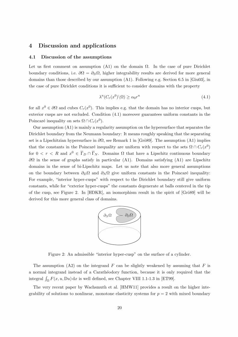
of the cusp, see Figure 2. In [HDKR], an isomorphism result in the spirit of [Gro89] will be

derived for this more general class of domains.

∂DΩ∂NΩ

Figure 2: An admissible “interior hyper-cusp” on the surface of a cylinder.

The assumption (A2) on the integrand F can be slightly weakened by assuming that F is

a normal integrand instead of a Caratheodory function, because it is only required that the

integral∫

Ω F (x, u,Du) dx is well defined, see Chapter VIII 1.1-1.3 in [ET99].

The very recent paper by Wachsmuth et al. [HMW11] provides a result on the higher inte-

grability of solutions to nonlinear, monotone elasticity systems for p = 2 with mixed boundary

20

conditions and it states invertibility properties of the corresponding differential operators in

W 1,p-spaces. We provide an exemplary energy density that satisfies the assumptions (A2)-(A3)

in our paper for p = 2, but is not included in the considerations in [HMW11].

Let p = n = N = 2 and assume pure Dirichlet boundary conditions, i.e. ∂Ω = ∂DΩ. Let the

energy density W : R2×2 → R be defined as

W (A) := 12 |A|2 + g(detA),

where g ∈ C2(R; [0,∞)) with g(1) = 0 and supa∈R |g′(a)| < ∞. Furthermore, g is convex,

nonlinear and satisfies for C > 0 and all a ∈ R the growth condition

g(a) ≤ C(1 + |a|).

The first summand of W , A 7→ 12 |A|2, is differentiable and strictly convex, whereas the second

summand A 7→ g(detA) is differentiable and quasi-convex, but no longer convex. There exists

c > 0 such that it holds for all A ∈ R2×2

12 |A|2 ≤W (A) ≤ 1

2 |A|2 + C(1 + | detA|) ≤ c(1 + |A|)2,

whatfrom (A2)-(A3) follow.

Let now u ∈ H10 (Ω) be a minimizer of the functional F , where

F(u) =

∫ΩW (∇u) dx.

Then there holds DF(u)[v] = 0 for all v ∈ H10 (Ω). The derivative of the energy density W is

given by

DW (A) =

A+ g′(detA) cof A, if det(A) 6= 0,

A, if det(A) = 0,

where cof A = detA ·A−T is the cofactor matrix. Hence, there holds for all v ∈ H10 (Ω)

0 = DF(u)[v] =

∫Ω

DW (∇u) : ∇v dx.

However, we now show that g can be chosen in such a way that DW : R2×2 → R2×2 is not

monotone and hence the analysis from [HMW11] cannot be applied here. Our Main Theorem

is applicable to F . Indeed, chose A1 = Id and A2 =(

0 − 12

1 0

). Then cof A1 = Id, detA1 = 1,

cof A2 =(

0 −112

0

), detA2 = 1

2 and we obtain with g′(1) = 0 that

(DW (A1)−DW (A2)) : (A1 −A2) =(

Id +g′(1) Id−(

0 − 12

1 0

)− g′(1

2)(

0 −112

0

)):(

112

−1 1

)= 13

4 + g′(12).

Now, for functions g as described above with g′(12) < −13

4 , the monotonicity condition from

[HMW11] is violated.

21

4.2 Damage of nonlinear elastic materials at small strains

In this section, we will show an application of the Main Theorem to a quasistatic evolution

model describing damage accumulation in an elastic body. In particular, we will prove on the

basis of Theorem 3.1 higher integrability of the deformation gradient ∇u, for the damage of

nonlinear elastic materials, presented in [TM10].

At first, we briefly recall the main aspects of the model: Let Ω ⊂ Rn and ∂DΩ ⊂ ∂Ω satisfy

assumption (A1) from Section 2 with λn−1(∂DΩ) > 0. The state space Q := U × Z is defined

for p, r ∈ (1,∞) by

U := W 1,pD (Ω;Rn) and Z := W 1,r(Ω).

We define the energy functional E : [0, T ]×Q → R by

E(t, u, z) :=

∫ΩW (x,∇u, z) + κ

r |∇z|r + χ[0,1](z) dx− 〈`(t), u〉, (4.2)

where κ > 0 is a material constant and ` ∈ C1([0, T ];W−1,p′(Ω;Rn)), 1p + 1

p′ = 1, represents the

volume and surface forces. The dissipation distance D : Z × Z → R∞ is defined as

D(z1, z2) :=

∫Ω ρ(x)(z1(x)− z2(x)) dx, if z2(x) ≤ z1(x) a.e.,

∞, else.(4.3)

There, ρ ∈ L∞(Ω) with 0 < ρ0 ≤ ρ almost everywhere is again a material dependent function

and can be interpreted as a kind of fracture toughness.

We aim to consider the constraint z ∈ [0, 1], whereby the value z = 1 corresponds to intact

material and z = 0 represents maximal damage. Due to the asymmetric definition of the

dissipation distance, the damage variable z is monotonically decreasing in time, as will be clear

from the evolution model (S) & (E), here below.

Hypotheses on the energy functional E:

(H1) Caratheodory function: W (x, ·, ·) ∈ C0(Rn×n × R) for almost every x ∈ Ω and

W (·, A, z) is measurable in Ω for all (A, z) ∈ Rn×n × R.

(H2) Quasi-convexity: For almost every x ∈ Ω and every z ∈ R the function A 7→W (x,A, z)

is quasi-convex.

(H3) p-growth and coercivity: For almost all x ∈ Ω and all z ∈ R we have W (x, ·, z) ∈C1(Rn×n) and there exists a constant C > 0 such that for almost every x ∈ Ω and every

(A, z) ∈ Rn×n × R we have W (x,A, z) ≤ C(1 + |A|p).Moreover, there exist W : Rn×n → R with W (0) = 0 and a constant ν > 0 such that for

every element u ∈ U there holds∫ΩW (∇u) dx ≥ ν

∫Ω|∇u|p dx

and for almost all x ∈ Ω and all (A, z) ∈ Rn×n × R it holds W (x,A, z) ≥ W (A).

22

(H4) Monotonicity: There exists constants k1 > 0, k2 ≤ 0 so that for almost every x ∈ Ω and

all (A, z), (A, z) ∈ Rd×dsym × [0, 1] with z ≤ z, we have

W (x,A, z) ≤W (x,A, z) ≤ k1(W (x,A, z) + k2).

Example for an admissible energy: For some δ ∈ (0, 1) let gδ : R→ R be defined as

gδ(z) :=

δ, if z < 0,

δ + (1− δ)z, if 0 ≤ z ≤ 1,

1, if z > 1.

Moreover, let C ∈ L∞(Ω; Lin(Rn×nsym ;Rn×nsym )) denote the elasticity tensor satisfying for some

constant ν > 0 and all e1, e2 ∈ Rn×nsym

Ce1 : e2 = Ce2 : e1 and Ce1 : e1 ≥ ν|e1|2. (4.4)

An exemplary energy density is then given by W (x,A, z) := 12gδ(z)C(x)Asym : Asym, where

Asym = 12(A+AT ) denotes the symmetric part. Then the energy

E(t, u, z) =

∫Ω

12gδ(z)Ce(u) : e(u) + κ

r |∇z|r + χ[0,1](z) dx− 〈`(t), u〉,

where e(u) = 12(∇u + ∇uT ) is the linearized strain tensor, satisfies (H1)-(H4) with p = 2 and

F (A) = |Asym|2.

Definition 4.1 (Energetic solution, Definition 2.1 in [TM10]). A pair (u, z) : [0, T ]→ Q is called

energetic solution for the rate-independent process (Q, E ,D), if t 7→ ∂tE(t, u(t), z(t)) ∈ L1(0, T )

and if for all t ∈ [0, T ] we have E(t, u(t), z(t)) <∞, stability (S) and energy balance (E):

(S) for all (u, z) ∈ Q holds: E(t, u(t), z(t)) ≤ E(t, u(t), z(t)) +D(z(t), z),

(E) E(t, u(t), z(t)) + DissD(z, [0, t]) = E(0, u(0), z(0)) +

∫ t

0∂tE(τ, u(τ), z(τ)) dτ,

where DissD(z, [0, t]) := sup∑M

j=1D(z(τj−1), z(τj)) and the supremum is taken over all partitions

of the interval [0, t].

An element (t, u, z) ∈ [0, T ]×Q such that (u, z) satisfies (S) in t is called stable. We will say

that (u, z) is a stable state at time t.

From the energy balance follows directly that there holds DissD(z, [0, t]) <∞ for all t ∈ [0, T ].

Hence, the asymmetric definition of the dissipation distance D implies that the damage variable

z is monotonically decreasing. In particular, there holds DissD(z; [0, t]) =∫

Ω ρ(z0 − z(t)) dx

for all monotonically decreasing functions z. Observe that, by setting z = z(t) in the stability

condition (S), we deduce

u(t) ∈ U(t, z(t)) := Argminv∈U

E(t, v, z(t)) = Argminv∈U

∫ΩW (x,∇v, z(t)) dx− 〈`(t), v〉 (4.5)

23

for all t ∈ [0, T ]. Since the term κr |∇z(t)|r is constant in v, we can neglect it while minimizing

with respect to v. Our damage model is a particular case of the model introduced in [TM10]

in the following sense: The hypothesis (H3) here is stronger than coercivity (H3)TM and stress

control (H4)TM in [TM10]: By (H2)-(H3), we find c > 0 such that there holds for almost all

x ∈ Ω and all (A, z) ∈ Rn×n × R that |∂AW (x,A, z)| ≤ c(1 + |A|p−1), which implies (H4)TM in

[TM10]. In [TM10, Theorem 3.1], the following existence result is shown:

Proposition 4.1 (Existence of energetic solutions). Let Q = U ×Z be defined as before, E as in

(4.2) with (H1)-(H4) and D as in (4.3). Then, for every stable initial state (u0, z0) ∈ Q, there

exists an energetic solution for the rate-independent process defined by (Q, E ,D).

As for the irreversibility of the damage process, it is clear that z(t) ≤ z0 ≤ 1 for all t ∈ [0, T ].

We will now proceed to prove the higher integrability of the deformation gradient ∇u.

Theorem 4.1 (Higher integrability for u). Assume that Ω ⊂ Rn satisfies (A1) and that the

external forces are of the form 〈`(t), v〉 =∫

ΩH0(t) ·v+H1(t) : ∇vdx with Hi ∈ C0([0, T ];Lr(Ω))

for some r > p. Then there exist constants q1 > p and c > 0 such that for all (t, z) ∈ [0, T ]×Zwith 0 ≤ z ≤ 1 and for all u ∈ U satisfying

u ∈ U(t, z) = Argminv∈U

∫ΩW (x,∇v, z) dx− 〈`(t), v〉,

it holds u ∈W 1,q1(Ω;Rn) and ‖u‖W 1,q1 (Ω) ≤ c.

Proof. We deduce the higher integrability for u by applying Theorem 3.1. Let (t, z) ∈ [0, T ]×Zbe arbitrarily fixed with 0 ≤ z ≤ 1, then u ∈ U(t, z) is a global minimizer of the functional

Ft(u) :=∫

ΩW (x,∇u, z) dx−〈`(t), u〉. The domain Ω satisfies (A1) by assumption. Due to (H1)

and (H3), the assumptions (A2)-(A3) are obviously satisfied for the energy density W . Due to

the assumptions on `, we can find uniform bounds, independent of t so that (A2)-(A3) hold

independently of t and z and Ft ∈ F(Ω, p, ν, c0, c1, b1, b2, γ) as given in Remark 2.1.

Since the Dirichlet boundary ∂DΩ has positive measure, 1 = γ < p and c1 = 0, we obtain from

Lemma 3.1 a uniform bound Cb ≥ 0 such that ‖u‖W 1,p(Ω) ≤ Cb for all t and z. The right-hand

side function b2 ≡ 1 ∈ L∞(Ω) is obviously higher integrable and therefore, Theorem 3.1 yields

u ∈W 1,q1(Ω;Rn) for some q1 > p.

This means in particular that for any energetic solution (u, z) the displacement satisfies

u(t) ∈W 1,q1(Ω;Rn) for all t ∈ [0, T ] and some q1 > p, independently of t and z.

4.3 Damage model without gradient of the damage variable

A further investigation of the damage model presented in [TM10] has been proposed in [FKS11],

where no nonlocal damage effects are present, and consequently no compactifying terms depen-

ding on the gradient of the damage variable appear in the energy functional. In this case, hard

24

technical difficulties prevent to obtain an existence result for the evolution in usual function

spaces. Instead, a Young measure evolution notion is presented, satisfying a weaker version of

the stability condition and a complete energy balance. We do not want to enter in the details of

this definition here, and we refer the interested reader to [FKS11, Definition 4.1]. We just recall

that, in order to perform the passage to the limit which provides the stability condition and

to obtain the lower energy estimate, the higher integrability of approximate strains is crucial,

and the related estimate is needed to be uniform with respect to the time-step chosen in the

approximation (see [FKS11, estimate (5.7)]). Whereas the uniform higher integrability is easily

obtained with the argument by Giaquinta and Giusti ([Giu03]) in the case where a fully Dirichlet

boundary condition is imposed and no external forces are present, the more general case of mixed

boundary conditions and external loads requires the higher integrability result proven in this

paper.

4.4 Phase transitions

It is also possible to apply Theorem 3.1 to the phase-transition model presented in [Fia10]. In

this paper a crystal material with finitely many phases and an elastic energy with quadratic

growth (p = 2) is considered. As in the damage case, we deal with the deformation gradient

∇v and an internal variable z, playing the role of a phase indicator. Since we consider a

multiphase material, a multiwell potential energy is to be expected. In [Fia10] no regularizing

term depending on the gradient of the internal variable z is considered, therefore the lack of

convexity of the energy functional is responsible for hard technical difficulties, which can be

overcome by considering a suitable notion of Young measure quasi-static evolution (see [Fia10,

Definition 6.2]).

In order to prove the convergence of the approximate solutions to a Young measure quasistatic

evolution, a suitable higher integrability property for the approximate deformation gradients

is needed (see [Fia10, Lemma 7.3]). This further regularity is proved in [Fia10] for a fully

Dirichlet boundary condition and no external forces, by applying the results by Giaquinta and

Giusti. Our higher integrability result allows us to consider the more general case of a Dirichlet

boundary condition imposed just on a part ∂DΩ of the boundary, and a nonzero external load

` ∈ C1([0, T ];W 1,1D (Ω)∗).

The proof of the desired higher integrability properties for the approximate deformation gra-

dients follows closely the argument in [Fia10, Lemma 7.2]. The reason why we need a more

regular external load than in the model analyzed in Section 4.2 is related to the fact that, in

the phase-transition case, Young measures need to be introduced from the very beginning in

the proof of the existence result, in order to construct approximate solutions. This makes the

application of the higher integrability result more delicate. In particular we need lower semicon-

tinuity of the functional u→ 〈`(t), u〉 with respect to the strong topology of W 1,1D (Ω), for every

t ∈ [0, T ], to apply Ekeland’s principle to the energy functional.

25

4.5 Higher integrability for a model describing shape memory alloys

As a further application of Theorem 3.1 we prove the uniform higher integrability of the stable

states related to a rate-independent model describing shape memory alloys. Let Ω ⊂ Rn satisfy

(A1) with λn−1(∂DΩ) > 0. Within the Souza-Auricchio model (see [SMZ98, AP02]) the state of a

shape memory material occupying the domain Ω is completely characterized by the displacement

field u : [0, T ]×Ω→ Rn and the internal variable z : [0, T ]×Ω→ Rn×ndev describing the mesoscopic

transformation strain. Here, Rn×ndev is the set of symmetric n × n tensors with vanishing trace.

Let the state space be given by Q = U ×Z with U = W 1,2D (Ω;Rn) and Z = W 1,2(Ω;Rn×ndev ). For

given time dependent loading ` ∈ C0([0, T ];U∗) and (v, ξ) ∈ U × Z the stored energy is defined

as

E(t, v, ξ) =

∫Ω

12C(e(v)− ξ) : (e(v)− ξ)dx− 〈`(t), v〉

+

∫Ω

g0(x)

2|∇z|2 + g1(x) |z|+ g2(x) |z|2 + χ(z)dx, (4.6)

where C ∈ L∞(Ω;R(n×n)×(n×n)) is the elasticity tensor satisfying the symmetry and positivity

properties from (4.4). Moreover, e(v) = 12(∇v +∇v>) denotes the linearized strain tensor. The

transformation strains z take their values in the compact, convex set Z =z ∈ Rn×ndev

∣∣ |z| ≤ σ0

,

where σ0 is a positive constant. This constraint enters into the energy functional through the

corresponding indicator function χ : Rn×ndev → 0,∞ with χ(ξ) = 0 if ξ ∈ Z and χ(ξ) = ∞otherwise. The energy that is dissipated when switching between different transformation strains

is taken into account via the dissipation functional R(ξ) =∫

Ω ρ(x) |ξ(x)| dx for ξ ∈ Z and fixed

ρ ∈ L∞(Ω) with ρ(x) ≥ ρ0 > 0 a.e. Analogously to the damage model discussed in Section

4.2, the pair (u, z) : [0, T ] → Q is called an energetic solution to the rate-independent process

defined by (Q, E ,R) if for all t it satisfies the stability condition (S) and the energy balance (E),

specified in Definition 4.1. The existence and uniqueness of energetic solutions is investigated

in [AMS08, MP07]. Here, we study the uniform higher integrability of the stable states. We

recall that a pair (u, z) ∈ U × Z is called a stable state at time t if (u, z) ∈ S(t), where the set

of stable states at time t is defined as

S(t) = (u, z) ∈ Q | E(t, u, z) ≤ E(t, v, ξ) +R(z − ξ) for all (v, ξ) ∈ Q.

Theorem 4.2. Assume that Ω ⊂ Rn satisfies (A1) and that the functions gi in (4.6) belong

to L∞(Ω) with gi(x) ≥ α > 0 for a.e. x and 0 ≤ i ≤ 2. Assume furthermore that the external

forces are of the form 〈`(t), v〉 =∫

ΩH0(t) · v + H1(t) : ∇vdx with Hi ∈ C0([0, T ];Lr(Ω)) for

some r > 2.

Then there exist q1, q2 > 2 and a constant c > 0 such that for all t ∈ [0, T ] and all stable states

(u, z) ∈ S(t) it holds u ∈W 1,q1(Ω;Rn), z ∈W 1,q2(Ω;Rn×ndev ) and ‖u‖W 1,q1 (Ω) + ‖z‖W 1,q2 (Ω) ≤ c.

In particular this theorem implies that energetic solutions of the Souza-Auricchio model are

higher integrable in space, uniformly in time.

26

Proof. First, we prove the higher integrability for the displacement field as in Section 4.2 and

subsequently for the internal variable. Observe that due to the stability condition (S) there

exists a constant Cb > 0 such that the uniform estimate

supt∈[0,T ],(u,z)∈S(t)

‖u‖W 1,2(Ω) + ‖z‖W 1,2(Ω) ≤ Cb (4.7)

is valid. Now in the same way as in the proof of Theorem 4.1 the uniform higher integrability

can be deduced for the displacement field u.

As for the higher integrability of z, we show that z can be interpreted as a Q-minimizer of

a suitable functional, and then apply again Theorem 3.1. For this we proceed in the spirit of

Example 6.4 in [Giu03]. Let (u, z) ∈ S(t) and let the functional Fu,z : W 1,2(Ω;Rn×ndev ) → R be

defined as

Fu,z(ξ) =

∫Ω

12C(e(u)− ξ) : (e(u)− ξ) + g1 |ξ|+ g2 |ξ|2 +

g0

2|∇ξ|2 dx+

∫Ωρ|z − ξ|dx

=

∫ΩFu,z(x, ξ) +

g0(x)

2|∇ξ|2 dx,

where Fu,z(x, ξ) = 12C(e(u(x))−ξ) : (e(u(x))−ξ)+g1 |ξ|+g2 |ξ|2+ρ|z(x)−ξ|. Since (u, z) ∈ S(t),

it holds

z ∈ ArgminFu,z(ξ) | ξ ∈W 1,2(Ω;Rn×ndev ), ξ(x) ∈ Z. (4.8)

Let now K ⊂ Rn be compact and η ∈W 1,2(Ω;Rn×ndev ) with η|Ω\K = z. We define η := PZ(η(x)),

where PZ : Rn×ndev → Z is the projection onto the convex and closed set Z. Observe that

η ∈ W 1,2(Ω;Rn×ndev ) with η|Ω\K = z and hence it is admissible for the minimization problem

(4.8). Therefore, with M := x ∈ Ω | η(x) ∈ Z the following estimate is valid:∫Ω∩K

Fu,z(x, z) +g0

2|∇z|2 dx ≤

∫Ω∩K

Fu,z(x, η) +g0

2|∇η|2 dx

=

∫Ω∩K∩M

Fu,z(x, η) +g0

2|∇η|2 dx+

∫(Ω∩K)\M

Fu,z(x, η) +g0

2|∇η|2 dx.

From the uniform bound (4.7) for u, the boundedness of the set Z and the Lipschitz continuity

of the projection PZ, it follows that there exist constants κ,C1 > 0, which are independent of

η, t, z and K such that∫(Ω∩K)\M

Fu,z(x, PZ(η)) +g0

2|∇PZ(η)|2dx ≤ κ

∫(Ω∩K)\M

C1(1 + |∇u|2) +g0

2|∇η|2dx.

Altogether it follows that∫Ω∩K

Fu,z(x, z) +g0

2|∇z|2dx ≤ (1 + κ)

∫Ω∩K

Fu,z(x, η) +g0

2|∇η|2 + C1(1 + |∇u|2)dx.

27

For x ∈ Ω and ξ ∈ Rn×ndev , we define F 0u,z(x, ξ) := Fu,z(x, ξ) + C1(1 + |∇u(x)|2). The above

calculations show that z is a Q-minimizer of (the functional)

F0u,z(η) :=

∫ΩF 0u,z(x, η) +

g0

2|∇η|2dx

with respect to W 1,2(Ω;Rn×ndev ) and for Q = 2 + κ. It can easily be checked that F0u,z satisfies

the assumptions of Theorem 3.1, which finishes the proof of Theorem 4.2.

Remark 4.1. The considerations can immediately be extended to quasiconvex energy densities

and with general compact, convex constraints Z ⊂ Rm, covering in this way the rate-independent

models studied in [FM06, Section 4].

A Appendix

Theorem A.1 (Poincare type inequality). Let Ω ⊂ Rn be a bounded domain with Lipschitz

boundary ∂Ω, p = pnn+p and uΩ the mean value defined by

uΩ :=1

|Ω|

∫Ωu dx = −

∫Qu dx.

Then there exists a constant CP > 0, only depending on n, p and Ω such that there holds for all

u ∈W 1,p(Ω;RN )

‖u− uΩ‖Lp(Ω) ≤ CP ‖Du‖Lp(Ω) .

Proof. See Theorem 3.15 in [Giu03].

Lemma A.1. Let p ≤ n, we define p∗ = pnn−p , if p < n and p∗ = γ(1+δ)

δ with γ, δ > 0 from (A2),

if p = n . There exists a constant Ce,P > 0 such that for all s ∈ (0, 12 ], y0 ∈ C+

1/2(0) (notation

from Section 3.1) it holds for all u ∈W 1,p(C+s (y0);RN )

‖u− uC+s (y0)‖Lp∗ (C+

s (y0)) ≤ Ce,P ‖Du‖Lp(C+s (y0)).

Proof. The proof relies on a scaling argument. For s ∈ (0, 12 ] and y0 ∈ C+

1/2(0), we define the

affine transformation Ts,y0 : C+1 → C+

s (y0) by

Ts,y0(x) := As,y0x+ bs,y0 ,

where As,y0 :=

s 0

. . ....

s 0

0 · · · 0 s+ miny0n, s

∈ Rn×n

and bs,y0 ∈ Rn is a suitable translation. Observe that it holds sn ≤ |det DTs,y0 | ≤ 2sn. Since we

have|det DTs,y0 ||C+s (y0)| =

sn−1(s+ miny0n, s)

(2s)n−1(s+ miny0n, s)

=1

2n−1=

1

|C+1 |,

28

the transformation formula reveals for the mean values that uC+s (y0) = (u Ts,y0)C+

1. By exploi-

ting the transformation formula, the embedding W 1,p(Ω;RN ) → Lp∗(Ω;RN ) and the classical

Poincare inequality, calculating the norm for p < n yields

‖u− uΩ‖p∗

Lp∗ (C+s )

=

∫C+

1

|u(Ts,y0(x))− (u Ts,y0)C+1|p∗ · | det DTs,y0 |dx

≤ 2Ce|s|n(∫

C+1

|u(Ts,y0(x))− (u Ts,y0)C+1|p + |Dxu(Ts,y0(x))|p dx

)p∗

p

≤ 2Ce,P |s|n(∫

C+1

|Dxu(Ts,y0(x))|p dx

)p∗

p

≤ 4Ce,P |s|n+p∗(∫

C+s

|Dyu(y)|p · | det DT−1s,y0| dy)p∗

p

≤ 4Ce,P ‖Du‖p∗

Lp(C+s ),

where n+ p∗ − np∗p = 0 . For p = n the last line reads Ce,P |s|n‖Du‖p∗

Lp(C+s )≤ 4Ce,P ‖Du‖p

∗

Lp(C+s )

,

since n+ p∗ − np∗p = n and s ≤ 1.

Theorem A.2 (Poincare-Friedrichs type inequality). Let Ω ⊂ Rn be a bounded domain with

Lipschitz boundary ∂Ω and p = pnn+p . Then, for every u ∈W 1,p(Ω) taking the value zero in a set

A ⊂ ∂Ω of positive measure, we have ‖u‖Lp(Ω) ≤ CP ‖Du‖Lp(Ω) , where CP is a positive constant

only depending on n, p,A and Ω.

Proof. See Theorem 5.4.3 in [ABM06].

Lemma A.2. Let ΓD be as introduced in Section 3 and p ≤ n. Then there exists a constant

Ce,P > 0 such that for all s ∈ (0, 12 ], y0 ∈ C+

1/2(0) with λn−1(Cs(y0)∩ΓD)λn−1(∂Cs(y0))

≥ κ0 > 0 it holds for all

u ∈W 1,p(C+s (y0);RN ) with u|ΓD = 0

‖u‖Lp∗ (C+s (y0)) ≤ Ce,P ‖Du‖Lp(C+

s (y0)).

Proof. According to the assumptions, we have

λn−1(Cs(y0) ∩ ΓD)

λn−1(∂Cs(y0))=

(2s)n−2hs,y0

c(n)(2s)n−1≥ κ0,

where c(n) is a dimension dependent constant and hs,y0 is the length of the Dirichlet boundary

projected on the y1-axis so that we arrive at hs,y0 ≥ 2κ0c(n). Thus, we find

A := y ∈ ΓD | y1 ≤ −1 + min1, 2κ0c(n) ⊂ T−1s,y0

(Cs(y

0) ∩ ΓD)⊂ ∂C+

1 (0),

with λn−1(A) ≥ min1, 2κ0c(n) > 0 independently of s and y0. The proof is now completely

analog to the one of Lemma A.1, if one applies Theorem A.2 instead of Theorem A.1.

29

Lemma A.3 (Lemma 6.1, [Giu03]). Let Z(t) be a bounded non-negative function in the interval

[ρ,R]. Assume that for ρ ≤ t < s ≤ R, we have

Z(t) ≤[A(s− t)−α +B(s− t)−β + C

]+ ϑZ(s)

with A,B,C ≥ 0, α > β > 0 and 0 ≤ ϑ < 1. Then

Z(ρ) ≤ c(α, ϑ)[A(R− ρ)−α +B(R− ρ)−β + C

].

Theorem A.3 (Giaquinta and Modica, Theorem 6.6 in [Giu03]). Let g, h ∈ L1(QR) with

g, h ≥ 0 almost everywhere and assume that for every pair of concentric cubes Q ⊂ Q ⊂⊂ QR,

where Q has the double diameter of Q, we have for some constant B > 0

−∫Qg dx ≤ B

(−∫Qgm dx

) 1m

+−∫Qh dx

, (A.1)

with 0 < m < 1. Assume the function h belongs to Ls(QR) for some s > 1. Then there exist

constants c > 0 and q > 1 such that g ∈ Lq(QR/2) and

−∫QR

2

gq dx ≤ c(−∫QR

g dx

)q+−∫QR

hq dx

. (A.2)

Remark A.1. As remarked in [NW91], a close inspection of the proof of Theorem 6.6 in [Giu03]

shows that the result remains valid if Q has six times the diameter of Q instead of two times.

The constant B in (A.1) is proportional to the Ciaccoppoli constant c from Corollary 3.1 with

B = B(c, n) ∼ 4nc and the constants c and q in (A.2) only depend on the parameters m and B

and not on local properties of the datum h.

References

[ABM06] H. Attouch, G. Buttazzo, and G. Michaille. Variational Analysis in Sobolev and BV Spaces.

MPS-SIAM Series on Optimization, 2006.

[AMS08] Ferdinando Auricchio, Alexander Mielke, and Ulisse Stefanelli. A rate-independent model for

the isothermal quasi-static evolution of shape-memory materials. Math. Models Methods Appl.

Sci., 18(1):125–164, 2008.

[AP02] Ferdinando Auricchio and Lorenza Petrini. Improvements and algorithmical considerations on

a recent three-dimensional model describing stress-induced solid phase transformations. Int.

J. Numer. Methods Eng., 55(11):1255–1284, 2002.

[ET99] I. Ekeland and R. Temam. Convex Analysis and Variational Problems. SIAM Classics In

Applied Mathematics, 1999.

[Fia10] A. Fiaschi. Rate-independent phase transitions in elastic materials: A Young-measure ap-

proach. Netw. Heterog. Media, 5(2):257–298, 2010.

30

[FKS11] A. Fiaschi, D. Knees, and U. Stefanelli. Young measure quasi-static damage evolution. Arch.

Ration. Mech. Anal., 2011. accepted.

[FM06] G. Francfort and A. Mielke. Existence results for a class of rate-independent material models

with nonconvex elastic energies. J. reine angew. Math., 595:55–91, 2006.

[GG82] M. Giaquinta and E. Giusti. On the regularity of the minima of variational integrals. Acta

Math., 148:31–46, 1982.

[Giu03] E. Giusti. Direct methods in the calculus of variations. Singapore: World Scientific, 2003.

[GM79] M. Giaquinta and G. Modica. Regularity results for some classes of higher order non linear

elliptic systems. J. Reine Angew. Math., 311-312:145–169, 1979.

[Gro89] K. Groger. A W 1,p-estimate for solutions to mixed boundary value problems for second order

elliptic differential equations. Math. Annalen, 283(4):679–687, 1989.

[HDKR] R. Haller-Dintelmann, D. Knees, and J. Rehberg. On function spaces related to mixed bound-

ary value problems. In preparation.

[HMW11] R. Herzog, C. Meyer, and G. Wachsmuth. Integrability of displacement and stresses in linear

and nonlinear elasticity with mixed boundary conditions. J. Math. Anal. Appl., 382(2):802–

813, 2011.

[KM06] J. Kristensen and G. Mingione. The singular set of minima of integral functionals. Arch.

Ration. Mech. Anal., 180(3):331–398, 2006.

[MP07] Alexander Mielke and Adrien Petrov. Thermally driven phase transformation in shape-memory

alloys. Adv. Math. Sci. Appl., 17(2):667–685, 2007.

[NW91] J. Naumann and M. Wolff. On a global Lq-gradient estimate on weak solutions of nonlinear

elliptic systems. Technical report, Dip. di Matematica, Universita degli Studi di Catania, 1991.

[Sim72] C.G. Simader. On Dirichlet’s boundary value problems, volume 268 of Lecture notes in Math-

ematics. Springer Verlag, 1972.

[SMZ98] Angela C. Souza, Edgar N. Mamiya, and Nestor Zouain. Three-dimensional model for solids

undergoing stress-induced phase transformations. Eur. J. Mech., A, Solids, 17(5):789–806,

1998.

[SW94] P. Shi and S. Wright. Higher integrability of the gradient in linear elasticity. Math. Ann.,

299(3):435–448, 1994.

[TM10] M. Thomas and A. Mielke. Damage of nonlinear elastic materials at small strain - existence

and regularity results -. Z. Angew. Math. Mech., 90:88–112, 2010.

[Zie89] W.P. Ziemer. Weakly Differentiable Functions. Springer-Verlag New York, 1989.

31