1

ENSC3003 – Fluid Mechanics

Semester 1, 2015

Week 2 Lecture Notes

Fluid Properties

© Dr Jeremy W. Leggoe February 2015

2

2.1 Momentum Transport In chemical engineering, the study of fluid mechanics is often regarded as one of the three “transport phenomena” courses (the other two being heat transfer, which deals with energy transport, and mass transfer, which deals with the transport of mass across phase interfaces and concentration gradients). One of the great chemical engineering textbooks, “Transport Phenomena”, by Bird, Stewart and Lightfoot (2002), combines the three transport courses into a single text. That text, which is on of the recommended texts for this unit is divided into three parts, and the part that deals with fluid mechanics is entitled “Momentum Transport”. This distinction is not necessarily intuitively obvious to many students. After all, in fluid mechanics we are often concerned with the movement of fluid masses, and the principle of conservation of mass is indeed still essential; the continuity equation, which derives from the principle of conservation of mass, is one of the fundamental equations governing fluid motion. To fully understand the way in which flow fields develop, however, it is essential to understand the manner in which momentum is transported within a fluid body. Momentum is transported in a fluid via molecular (or in some cases atomic) interactions Consider a solid body, such as a pen. If you hold one end of the pen and start to move it by moving your fingers, the remainder of the pen translates along with the portion where your fingers are in contact with the pen. Momentum is transported with more or less perfect efficiency along the pen, due to the effectively rigid bonds between the molecules in the materials that make up the pen. In other words, if you move one end of the pen, the rest of the pen comes along at the same velocity. Now consider a fluid – say, water in a pot or a bowl. If you put a spoon into the water and move it, the water immediately adjacent to the spoon will move immediately, but the water further from the spoon will move later (if at all), and with diminished velocity. In the absence of significant bonding between molecules, momentum is transported less efficiently than in a solid body, but it is still transferred as individual molecules interact with those adjacent to them. Consider two adjacent layers of fluid moving at different velocities (U and U+dU), as in figure 2.1 overleaf. The faster moving molecules in the upper layer will interact with the slower molecules in the lower layer, imparting momentum. Thus momentum is “transported” from the faster moving fluid to the slower moving fluid. It can be seen that wherever a velocity gradient exists, momentum will be transported – and it will be transported in the direction of decreasing velocity.

3

Figure 2.1 The faster moving molecules in the upper layer impart momentum to the slower moving molecules in the adjacent layer through molecular interactions. Thus, momentum is transported from the faster moving fluid to the slower moving fluid. Momentum is transported in the direction of decreasing velocity.

2.2 Viscosity The viscosity of a fluid characterizes the efficiency with which a fluid is able to transport momentum. Naturally, viscosity will depend on the intensity and frequency of the molecular interactions within a fluid – as can be seen from the typical viscosity values presented in Table 1 below. As you would expect, solids exhibit the highest viscosity. Liquid viscosities vary widely, depending on the nature of the molecules in the liquid and the nature of their interactions (entanglement, polarity, etc). Gas viscosities are relatively low, and are orders of magnitude lower than those exhibited by liquids, as would be expected given the much wider spacing of gas molecules. One intuitive way to think of viscosity is to think of it as characterising the resistance to flow exhibited by a fluid – “the more viscous a fluid is, the harder it is to make it flow”. This is a logical alternative way of thinking, given that the slower moving molecules do draw momentum from the faster moving particles, diminishing their ability to move freely and reducing “flow”. It is important, though to remember that this is just another way of thinking about the momentum transport that is happening.

4

Phase Viscosity

Range Pa.s

Description

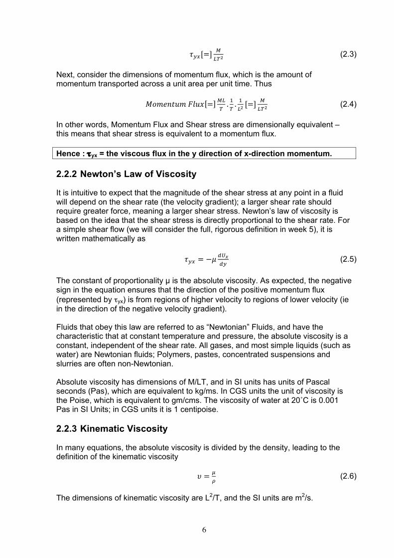
Solid Up to ≈∞ Rigid bonds give virtually perfect momentum transport in many materials – but many glasses (polymer and ceramic) exhibit high but finite viscosities, and flow slowly

Liquid 100 – 10-2 High viscosity liquids – polymers such as glycerol (0.9 Pas), which have long entangled chains, high density fluids such as Mercury and sulphuric acid (2.5 x 10-2 Pas).

10-3 – 10-4 Moderate viscosity – low molecular weight liquids, such as water (10-3 Pas at room temperature) and butanol (2.8 x 10-4 Pas at room temperature)

Gas 10-4 – 10-6 Low viscosity – widely separated molecules, (relatively) infrequent interactions. Sample values – Isobutane: 8 x 10-6 Pas at standard atmospheric conditions (SAC), Air: 1.8 x 10-5 Pas at SAC

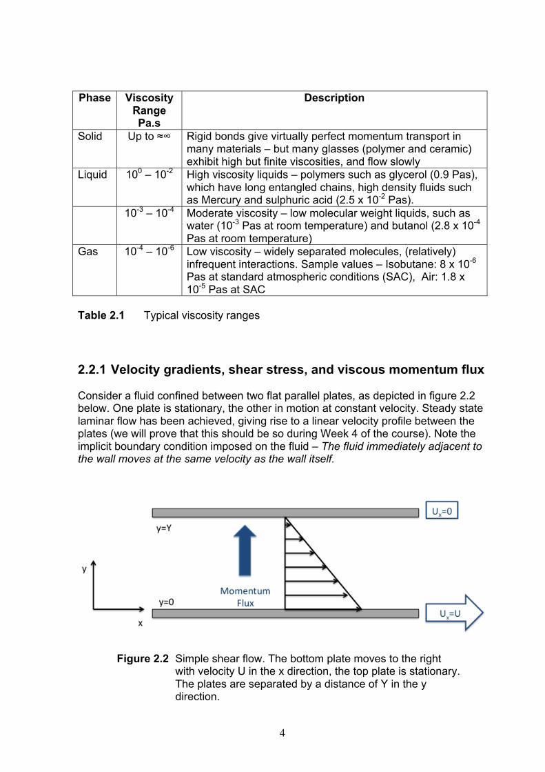
Table 2.1 Typical viscosity ranges 2.2.1 Velocity gradients, shear stress, and viscous momentum flux Consider a fluid confined between two flat parallel plates, as depicted in figure 2.2 below. One plate is stationary, the other in motion at constant velocity. Steady state laminar flow has been achieved, giving rise to a linear velocity profile between the plates (we will prove that this should be so during Week 4 of the course). Note the implicit boundary condition imposed on the fluid – The fluid immediately adjacent to the wall moves at the same velocity as the wall itself.

Figure 2.2 Simple shear flow. The bottom plate moves to the right with velocity U in the x direction, the top plate is stationary. The plates are separated by a distance of Y in the y direction.

5

Given a linear velocity profile, the velocity gradient, or “shear rate” is given by: !!!

!"= − !

! (2.1)

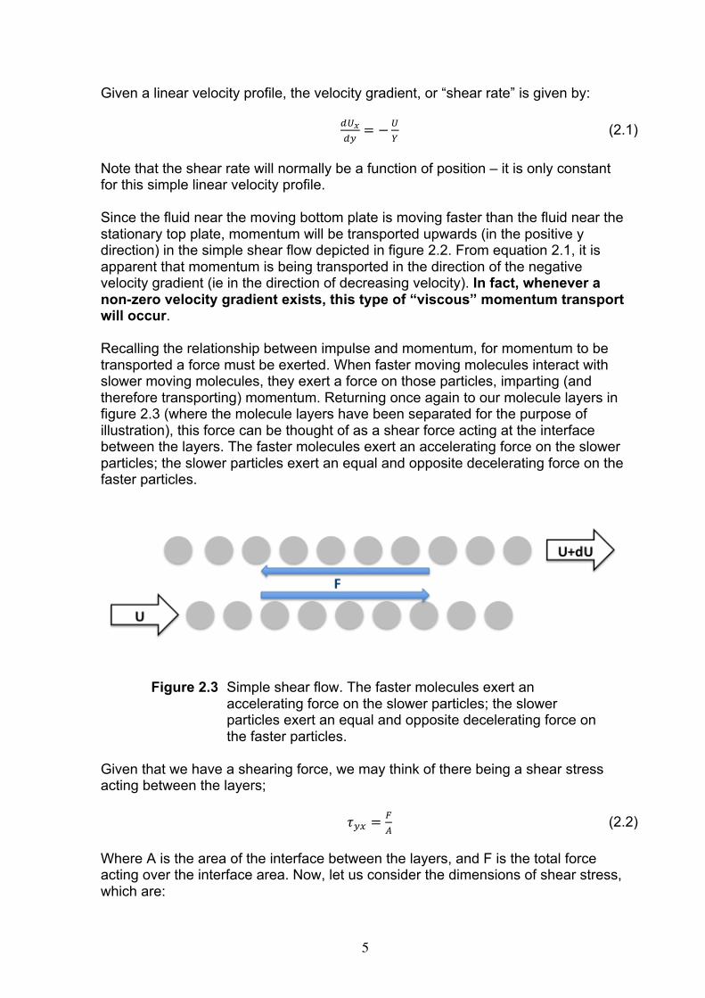
Note that the shear rate will normally be a function of position – it is only constant for this simple linear velocity profile. Since the fluid near the moving bottom plate is moving faster than the fluid near the stationary top plate, momentum will be transported upwards (in the positive y direction) in the simple shear flow depicted in figure 2.2. From equation 2.1, it is apparent that momentum is being transported in the direction of the negative velocity gradient (ie in the direction of decreasing velocity). In fact, whenever a non-zero velocity gradient exists, this type of “viscous” momentum transport will occur. Recalling the relationship between impulse and momentum, for momentum to be transported a force must be exerted. When faster moving molecules interact with slower moving molecules, they exert a force on those particles, imparting (and therefore transporting) momentum. Returning once again to our molecule layers in figure 2.3 (where the molecule layers have been separated for the purpose of illustration), this force can be thought of as a shear force acting at the interface between the layers. The faster molecules exert an accelerating force on the slower particles; the slower particles exert an equal and opposite decelerating force on the faster particles.

Figure 2.3 Simple shear flow. The faster molecules exert an accelerating force on the slower particles; the slower particles exert an equal and opposite decelerating force on the faster particles.

Given that we have a shearing force, we may think of there being a shear stress acting between the layers; 𝜏!" =

!! (2.2)

Where A is the area of the interface between the layers, and F is the total force acting over the interface area. Now, let us consider the dimensions of shear stress, which are:

6

𝜏!"[=]!!!!

(2.3) Next, consider the dimensions of momentum flux, which is the amount of momentum transported across a unit area per unit time. Thus 𝑀𝑜𝑚𝑒𝑛𝑡𝑢𝑚  𝐹𝑙𝑢𝑥 = !"

!. !!. !!![=] !

!!! (2.4)

In other words, Momentum Flux and Shear stress are dimensionally equivalent – this means that shear stress is equivalent to a momentum flux. Hence : τyx = the viscous flux in the y direction of x-direction momentum. 2.2.2 Newton’s Law of Viscosity It is intuitive to expect that the magnitude of the shear stress at any point in a fluid will depend on the shear rate (the velocity gradient); a larger shear rate should require greater force, meaning a larger shear stress. Newton’s law of viscosity is based on the idea that the shear stress is directly proportional to the shear rate. For a simple shear flow (we will consider the full, rigorous definition in week 5), it is written mathematically as 𝜏!" = −𝜇 !!!

!" (2.5)

The constant of proportionality µ is the absolute viscosity. As expected, the negative sign in the equation ensures that the direction of the positive momentum flux (represented by τyx) is from regions of higher velocity to regions of lower velocity (ie in the direction of the negative velocity gradient). Fluids that obey this law are referred to as “Newtonian” Fluids, and have the characteristic that at constant temperature and pressure, the absolute viscosity is a constant, independent of the shear rate. All gases, and most simple liquids (such as water) are Newtonian fluids; Polymers, pastes, concentrated suspensions and slurries are often non-Newtonian. Absolute viscosity has dimensions of M/LT, and in SI units has units of Pascal seconds (Pas), which are equivalent to kg/ms. In CGS units the unit of viscosity is the Poise, which is equivalent to gm/cms. The viscosity of water at 20˚C is 0.001 Pas in SI Units; in CGS units it is 1 centipoise. 2.2.3 Kinematic Viscosity In many equations, the absolute viscosity is divided by the density, leading to the definition of the kinematic viscosity 𝜐 = !

! (2.6)

The dimensions of kinematic viscosity are L2/T, and the SI units are m2/s.

7

2.2.4 Non-Newtonian Fluids For most of this course, we will deal with Newtonian fluids, BUT as mentioned previously there are fluids of practical importance that are not Newtonian. Analysis of non-Newtonian fluid flow is a matter for advanced courses in transport phenomena, but it is important to be aware of the various types of non-Newtonian behaviour. A generalized definition of viscosity may be written as: 𝜏!" = −𝜂 !!!

!" (2.7)

Now η is not a constant, independent of the shear rate – it can be a function of the shear stress and the shear rate.

Figure 2.4 Schematic plots of shear stress vs shear rate for Newtonian and non-Newtonian fluids.

8

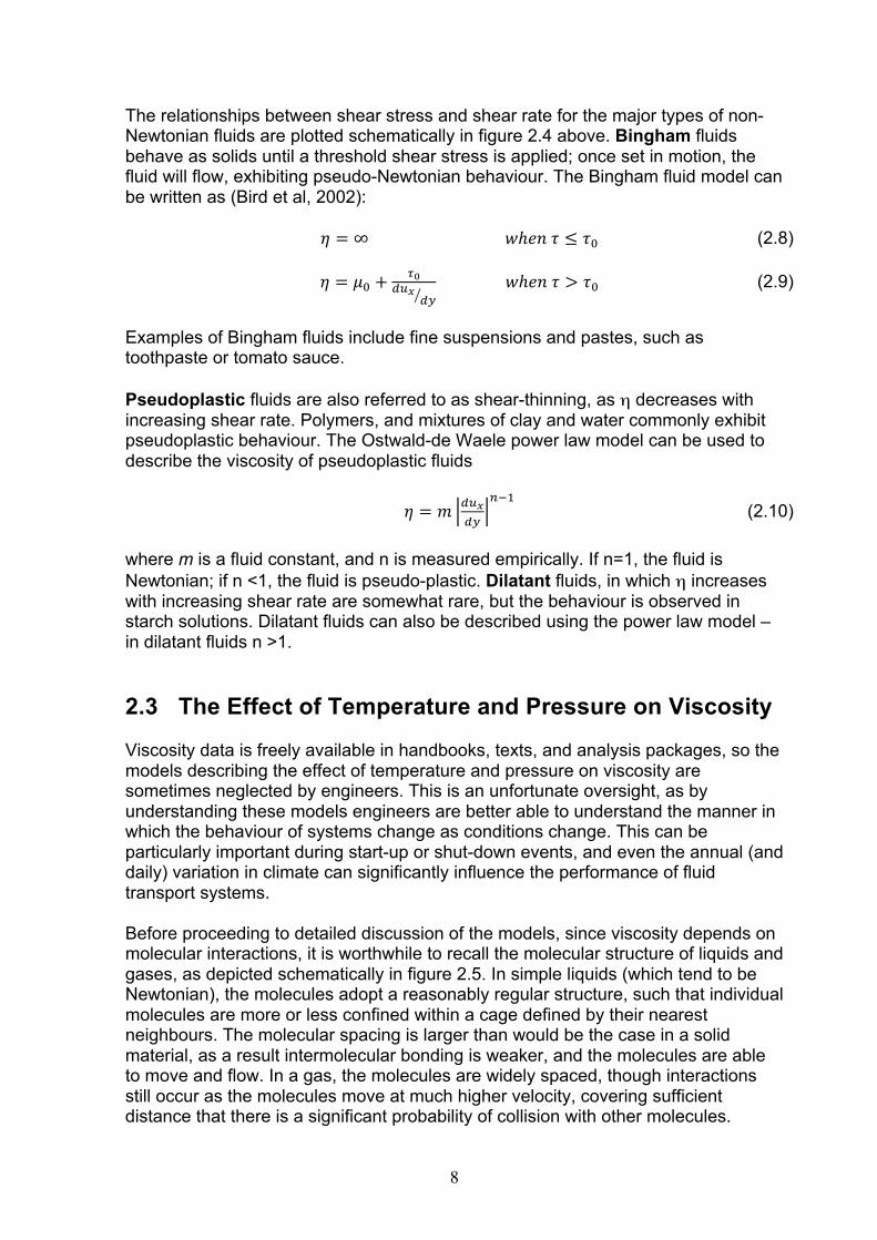
The relationships between shear stress and shear rate for the major types of non-Newtonian fluids are plotted schematically in figure 2.4 above. Bingham fluids behave as solids until a threshold shear stress is applied; once set in motion, the fluid will flow, exhibiting pseudo-Newtonian behaviour. The Bingham fluid model can be written as (Bird et al, 2002): 𝜂 = ∞                                                                      𝑤ℎ𝑒𝑛  𝜏 ≤ 𝜏! (2.8) 𝜂 = 𝜇! +

!!!"!

!"                                  𝑤ℎ𝑒𝑛  𝜏 > 𝜏! (2.9)

Examples of Bingham fluids include fine suspensions and pastes, such as toothpaste or tomato sauce. Pseudoplastic fluids are also referred to as shear-thinning, as η decreases with increasing shear rate. Polymers, and mixtures of clay and water commonly exhibit pseudoplastic behaviour. The Ostwald-de Waele power law model can be used to describe the viscosity of pseudoplastic fluids

𝜂 = 𝑚 !"!!"

!!! (2.10)

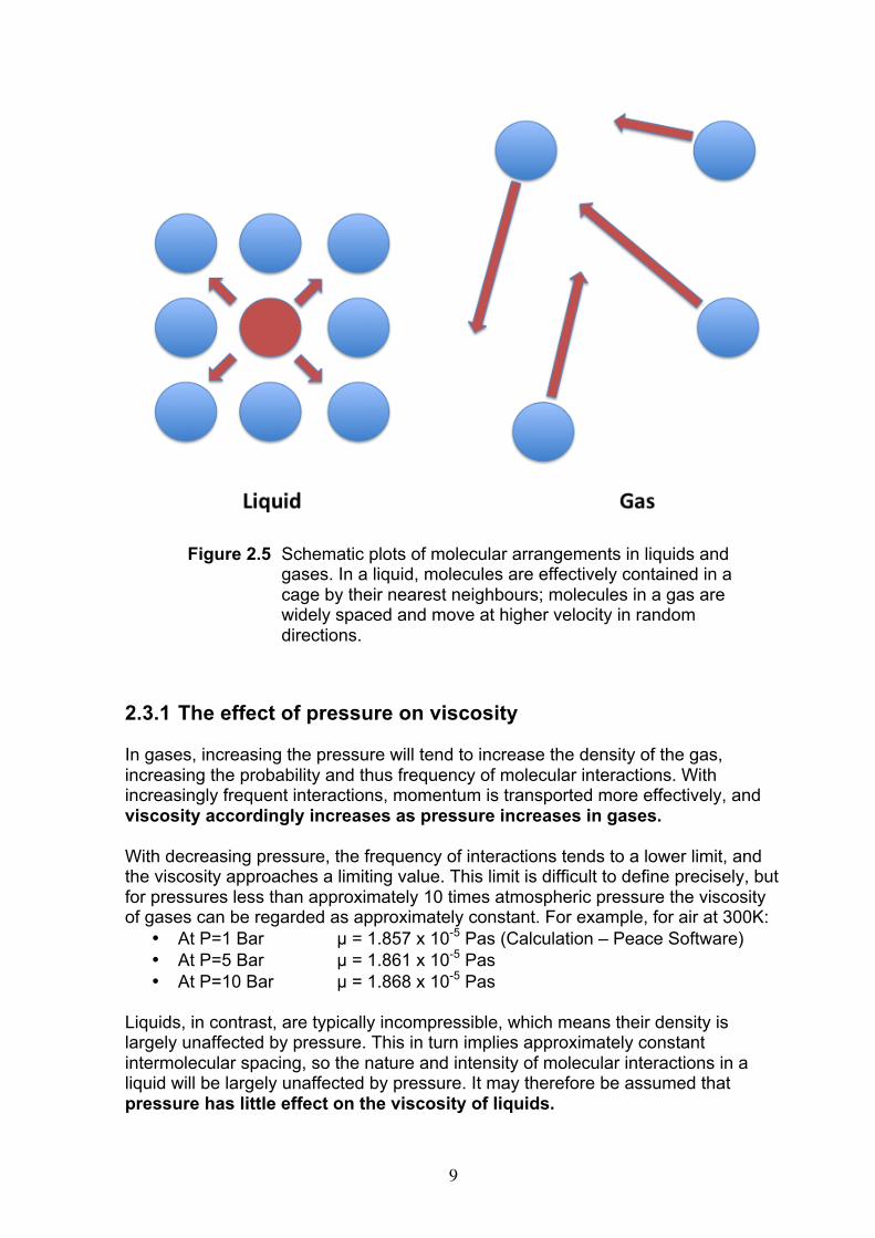
where m is a fluid constant, and n is measured empirically. If n=1, the fluid is Newtonian; if n <1, the fluid is pseudo-plastic. Dilatant fluids, in which η increases with increasing shear rate are somewhat rare, but the behaviour is observed in starch solutions. Dilatant fluids can also be described using the power law model – in dilatant fluids n >1. 2.3 The Effect of Temperature and Pressure on Viscosity Viscosity data is freely available in handbooks, texts, and analysis packages, so the models describing the effect of temperature and pressure on viscosity are sometimes neglected by engineers. This is an unfortunate oversight, as by understanding these models engineers are better able to understand the manner in which the behaviour of systems change as conditions change. This can be particularly important during start-up or shut-down events, and even the annual (and daily) variation in climate can significantly influence the performance of fluid transport systems. Before proceeding to detailed discussion of the models, since viscosity depends on molecular interactions, it is worthwhile to recall the molecular structure of liquids and gases, as depicted schematically in figure 2.5. In simple liquids (which tend to be Newtonian), the molecules adopt a reasonably regular structure, such that individual molecules are more or less confined within a cage defined by their nearest neighbours. The molecular spacing is larger than would be the case in a solid material, as a result intermolecular bonding is weaker, and the molecules are able to move and flow. In a gas, the molecules are widely spaced, though interactions still occur as the molecules move at much higher velocity, covering sufficient distance that there is a significant probability of collision with other molecules.

9

Figure 2.5 Schematic plots of molecular arrangements in liquids and gases. In a liquid, molecules are effectively contained in a cage by their nearest neighbours; molecules in a gas are widely spaced and move at higher velocity in random directions.

2.3.1 The effect of pressure on viscosity In gases, increasing the pressure will tend to increase the density of the gas, increasing the probability and thus frequency of molecular interactions. With increasingly frequent interactions, momentum is transported more effectively, and viscosity accordingly increases as pressure increases in gases. With decreasing pressure, the frequency of interactions tends to a lower limit, and the viscosity approaches a limiting value. This limit is difficult to define precisely, but for pressures less than approximately 10 times atmospheric pressure the viscosity of gases can be regarded as approximately constant. For example, for air at 300K:

• At P=1 Bar µ = 1.857 x 10-5 Pas (Calculation – Peace Software) • At P=5 Bar µ = 1.861 x 10-5 Pas • At P=10 Bar µ = 1.868 x 10-5 Pas

Liquids, in contrast, are typically incompressible, which means their density is largely unaffected by pressure. This in turn implies approximately constant intermolecular spacing, so the nature and intensity of molecular interactions in a liquid will be largely unaffected by pressure. It may therefore be assumed that pressure has little effect on the viscosity of liquids.

10

2.3.2 The effect of temperature on viscosity For gases at low pressure (ie around atmospheric pressure), the viscosity of a gas will increase with increasing temperature. This can be understood by considering the effect of temperature on molecular motion. Increasing the temperature of a gas will increase the velocity of the molecules, increasing the mean free path travelled by the molecules, and therefore increasing the probability of molecular interactions. Increasing the incidence of molecular interactions increases the effectiveness of momentum transport, thereby increasing the viscosity. The viscosity of gases at low pressure (<10 atm) can be predicted using the Chapman-Enskog equation (Bird et al, 2002). The equation was derived for monatomic gases, but works reasonably well for polyatomic gases, and is given by: 𝜇 = 2.6693×10!! !!!

!!!! (2.11)

Where • Mw is molecular weight (in gm/mol) • T is the absolute temperature (in K) • σ is the collision diameter (in Angstroms) • Ωµ is the collision integral

The last two quantities must be determined from tables in the literature – they are available in Tables E1 and E2 in Bird, Stewart and Lightfoot (2002). Written in this form, the equation gives an answer in Pas, as long as the correct units are used for each of the variables. Note that the constant is not dimensionless, so different values are needed for different unit combinations (the text “Transport Phenomena”, for example, uses a different constant that yields viscosity in Poise). It appears from the equation that the viscosity is roughly proportional to the square root of the temperature; in fact once the effect of temperature on the other variables is taken into account it turns out the viscosity is proportional to between T0.6 and T1.0, depending on the temperature and the gas in question. Determining the viscosity of mixtures of gases is also of practical importance – for starters, atmospheric air is a mixture of gases. For mixtures of gases at low pressure (ie around atmospheric pressure) the viscosity of a gas mixture having N components can be estimated using: 𝜇!"# =

!!!!!!!!"!

!

!! (2.12)

where xi is the mole fraction of component i of the mixture, and the interaction parameter φij is given by

𝜙!" =!!1+ !!

!!

!!/!1+ !!

!!

!/! !!

!!

!/! !

(2.13)

Mi is the molecular weight of component i of the mixture.

11

The effect of temperature on the viscosity of liquids can be estimated using the Eyring equation [Bird et al, 2002]:

𝜇 = !!!𝑒!.!

!!! (2.14)

Where

• 𝑁 is Avogadro’s Number (6.023 x 1023) • h is the Planck Constant (6.626 x 10-34 J/s) • 𝑉 is the specific molar volume • Tb is the boiling temperature of the liquid (in K) • T is the temperature of the liquid (in K)

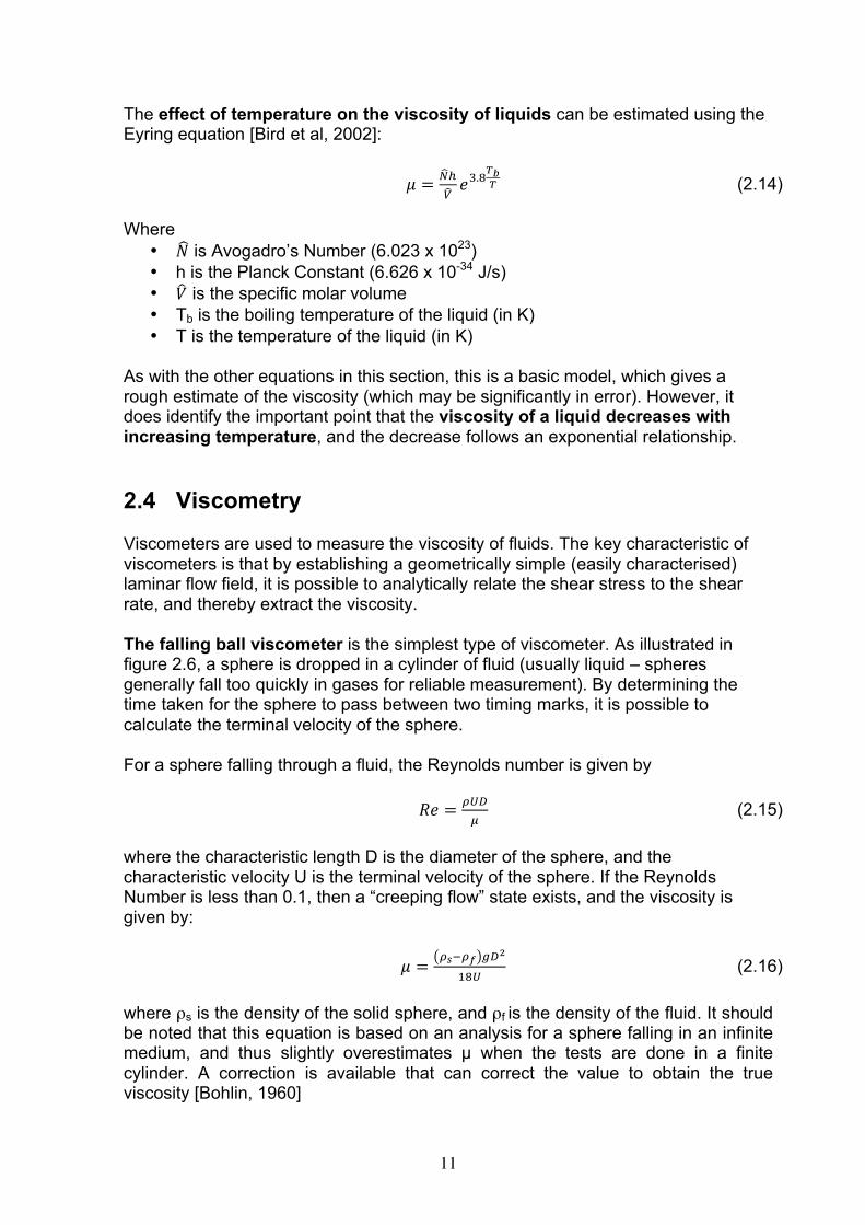
As with the other equations in this section, this is a basic model, which gives a rough estimate of the viscosity (which may be significantly in error). However, it does identify the important point that the viscosity of a liquid decreases with increasing temperature, and the decrease follows an exponential relationship. 2.4 Viscometry Viscometers are used to measure the viscosity of fluids. The key characteristic of viscometers is that by establishing a geometrically simple (easily characterised) laminar flow field, it is possible to analytically relate the shear stress to the shear rate, and thereby extract the viscosity. The falling ball viscometer is the simplest type of viscometer. As illustrated in figure 2.6, a sphere is dropped in a cylinder of fluid (usually liquid – spheres generally fall too quickly in gases for reliable measurement). By determining the time taken for the sphere to pass between two timing marks, it is possible to calculate the terminal velocity of the sphere. For a sphere falling through a fluid, the Reynolds number is given by 𝑅𝑒 = !"#

! (2.15)

where the characteristic length D is the diameter of the sphere, and the characteristic velocity U is the terminal velocity of the sphere. If the Reynolds Number is less than 0.1, then a “creeping flow” state exists, and the viscosity is given by: 𝜇 = !!!!! !!!

!"! (2.16)

where ρs is the density of the solid sphere, and ρf is the density of the fluid. It should be noted that this equation is based on an analysis for a sphere falling in an infinite medium, and thus slightly overestimates µ when the tests are done in a finite cylinder. A correction is available that can correct the value to obtain the true viscosity [Bohlin, 1960]

12

Figure 2.6 Schematic illustration of a falling ball viscometer, where a solid sphere of diameter D falls in a cylinder of diameter d. Terminal velocity is determined by measuring the time taken for the sphere to fall a defined distance L.

A capillary viscometer uses a tube of small diameter, in which it is easier to maintain a laminar flow, to measure viscosity. For a laminar flow in a tube there are simple analytical relationships relating the pressure loss to the volume flow rate and the fluid viscosity. Examples include the Cannon-Fenske (two tube) and Ubbelohde (3 tube) viscometers, in which the time taken for the fluid to drain out of a capillary tube is measured. This is then converted into a viscosity using calibration charts established for the individual viscometer being used (Each viscometer design has its own calibration). To design a capillary viscometer, it is essential to ensure a laminar flow. This is done by ensuring that the Reynolds number for the flow is less than 2000. For a capillary tube: 𝑅𝑒 = !"#

! (2.17)

where the characteristic length D is the diameter of the tube, and the characteristic velocity U is the average velocity of the flow in the tube. For a vertical tube (the usual test configuration), the volume flow rate in the tube is given by: 𝑄 = !!! !!!!!!  !"#

!"#!" (2.18)

where the L is the length of the tube, and Po and PL are the pressures at the inlet and outlet of the tube.

13

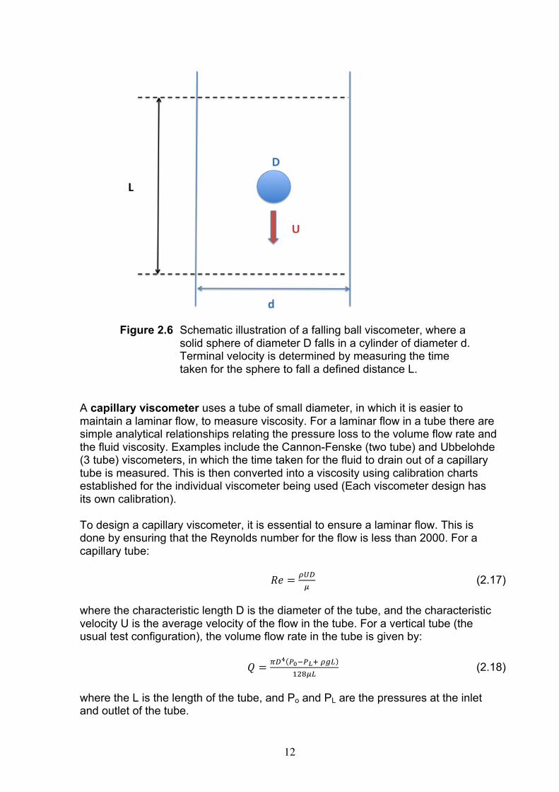
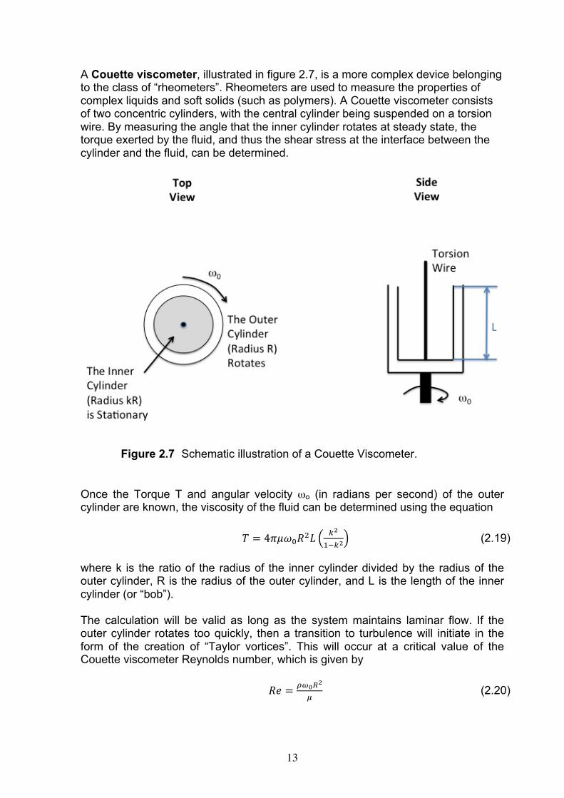
A Couette viscometer, illustrated in figure 2.7, is a more complex device belonging to the class of “rheometers”. Rheometers are used to measure the properties of complex liquids and soft solids (such as polymers). A Couette viscometer consists of two concentric cylinders, with the central cylinder being suspended on a torsion wire. By measuring the angle that the inner cylinder rotates at steady state, the torque exerted by the fluid, and thus the shear stress at the interface between the cylinder and the fluid, can be determined.

Figure 2.7 Schematic illustration of a Couette Viscometer. Once the Torque T and angular velocity ωo (in radians per second) of the outer cylinder are known, the viscosity of the fluid can be determined using the equation 𝑇 = 4𝜋𝜇𝜔!𝑅!𝐿

!!

!!!! (2.19)

where k is the ratio of the radius of the inner cylinder divided by the radius of the outer cylinder, R is the radius of the outer cylinder, and L is the length of the inner cylinder (or “bob”). The calculation will be valid as long as the system maintains laminar flow. If the outer cylinder rotates too quickly, then a transition to turbulence will initiate in the form of the creation of “Taylor vortices”. This will occur at a critical value of the Couette viscometer Reynolds number, which is given by 𝑅𝑒 = !!!!!

! (2.20)

14

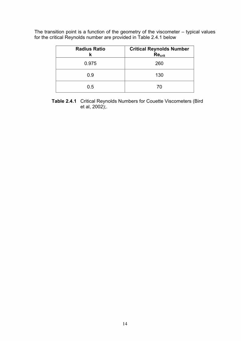
The transition point is a function of the geometry of the viscometer – typical values for the critical Reynolds number are provided in Table 2.4.1 below

Radius Ratio k

Critical Reynolds Number Recrit

0.975 260

0.9 130

0.5 70

Table 2.4.1 Critical Reynolds Numbers for Couette Viscometers (Bird

et al, 2002);.

15

References R.B. Bird, W.E. Stewart & E.N. Lightfoot, “Transport phemonena”, Second Edition, John Wiley and Sons, New York, 2002 T. Bohlin, “Terminal velocities of solid spheres in cylindrical enclosures”, Transactions of the Royal Institute of Technology, Stockholm, Report #155, 1960