niasra.uow.edu.auweb/@inf/@math/... · Submitted to the Annals of Statistics arXiv: math.PR/0000000...

Copyright © 2008 by the Centre for Statistical & Survey Methodology, UOW. Work in progress, no part of this paper may be reproduced without permission from the Centre.

Centre for Statistical & Survey Methodology, University of Wollongong, Wollongong NSW 2522. Phone +61 2 4221 5435, Fax +61 2 4221 4845. Email: [email protected]

Centre for Statistical and Survey Methodology

The University of Wollongong

Working Paper

04-10

ASYMPTOTIC NORMALITY AND VALID INFERENCE FOR

GAUSSIAN VARIATIONAL APPROXIMATION

Hall, P., Pham, T., Wand,M.P. and Wang, S.S.J.

Submitted to the Annals of StatisticsarXiv: math.PR/0000000

ASYMPTOTIC NORMALITY AND VALID INFERENCE FOR GAUSSIAN

VARIATIONAL APPROXIMATION

By Peter Hall ∗, Tung Pham † M.P. Wand †

and S.S.J. Wang †

University of Melbourne∗ and University of Wollongong†

9th November, 2010

We derive the precise asymptotic distributional behavior of Gaus-sian variational approximate estimators of the parameters in a single-predictor Poisson mixed model. These results are the deepest yetobtained concerning the statistical properties of a variational ap-proximation method. Moreover, they give rise to asymptotically validstatistical inference. A simulation study demonstrates that Gaussianvariational approximate confidence intervals possess good to excel-lent coverage properties, and with precision similar to their exactlikelihood counterparts.

1. Introduction. Variational approximation methods are enjoying an increasing amountof development and use in statistical problems. This raises questions regarding their statisticalproperties, such as consistency of point estimators and validity of statistical inference. We makesignificant inroads into answering such questions via thorough theoretical treatment of one ofthe simplest non-trivial settings for which variational approximation is beneficial: the Poissonmixed model with a single predictor variable and random intercept. We call this the modelsimple Poisson mixed model.

The model treated here is also treated in [5], but there attention is confined to bounds andrates of convergence. We improve upon their results by obtaining the asymptotic distributions ofthe estimators. The results reveal that the estimators are asymptotically normal, have negligiblebias, and that their variances decay at least as fast as m−1, where m is the number of groups.For the slope parameter, the faster (mn)−1 rate is obtained, where n is the number of repeatedmeasures.

An important practical ramification of our theory is asymptotically valid statistical inferencefor the model parameters. In particular, a form of studentization leads to theoretically justifi-able confidence intervals for all model parameters. Unlike those based on the exact likelihood,all Gaussian variational approximate point estimates and confidence intervals can be computedwithout the need for numerical integration. Simulation results reveal that the confidence inter-vals have good to excellent coverage and have about the same length as exact likelihood-basedintervals.

Variational approximation methodology is now a major research area with Computer Science;see, for example, Chapter 10 of [2]. It is beginning to have a presence in Statistics as well (e.g.[8], [11]) A summary of the topic from a statistical perspective is given in [10]. Late 2010saw the first non-beta release of a software library, Infer.NET [9], for facilitation of variationalapproximate inference. A high proportion of variational approximation methodology is framedwithin Bayesian hierarchical structures and offers itself as a faster alternative to Markov chainMonte Carlo methods. The chief driving force is applications where speed is at a premium andsome accuracy can be sacrificed. Examples of such applications are cluster analysis of gene-expression data [13], fitting spatial models to neuroimage data [4], image segmentation [3] and

AMS 2000 subject classifications: Primary 62F12; secondary 62F25Keywords and phrases: Generalized linear mixed models, Longitudinal data analysis, Maximum likelihood es-

timation, Poisson mixed models

1

2 P. HALL, T. PHAM, M.P. WAND AND S.S.J. WANG

genome-wide association analysis [6].As explained in [2] and [10], there are many types of variational approximations. The most

popular is variational Bayes (also known as mean field approximation), which relies on productrestrictions applied to the joint posterior densities of a Bayesian model. The present article isconcerned with Gaussian variational approximation in frequentist models containing randomeffects. There are numerous models of this general type. One of their hallmarks is the difficultyof exact likelihood-based inference for the model parameters due to presence of non-analyticintegrals. Generalized linear mixed models (e.g. Chapter 7 of [7]) form a large class of modelsfor handling within-group correlation when the response variable is non-Gaussian. The simplePoisson mixed model lies within this class. From a theoretical standpoint, the simple Poissonmixed model is attractive because it possesses the computational challenges that motivate Gaus-sian variational approximation — exact likelihood-based inference requires quadrature — butits simplicity makes it amenable to deep theoretical treatment. We take advantage of this sim-plicity to derive the asymptotic distribution of the Gaussian variational approximate estimators,although the derivations are still quite intricate and involved. These results represent the deepeststatistical theory yet obtained for a variational approximation method.

Moreover, for the first time, asymptotically valid inference for a variational approximationmethod is manifest. Our theorem reveals that each estimator is asymptotically normal, centeredon the true parameter value and with a studentizable variance. Replacement of the unknownquantities by consistent estimators results in asymptotically valid confidence intervals and Waldhypothesis tests. A simulation study shows that Gaussian variational approximate confidenceintervals possess good to excellent coverage properties — especially in the case of the slopeparameter.

Section 2 describes the simple Poisson mixed model and Gaussian variational approximation.An asymptotic normality theorem is presented in Section 3. In Section 4 we discuss the implica-tions for valid inference and perform some numerical evaluations. Section 5 contains the proofof the theorem.

2. Gaussian variational approximation for the simple Poisson mixed model. Thesimple Poisson mixed model that we study here is identical to that treated in [5]. Section 2 ofthat paper provides a detailed description of the model and the genesis of Gaussian variationalapproximation for estimation of the model parameters. Here we give just a rudimentary accountof the model and estimation strategy.

The simple Poisson mixed model is

Yij |Xij , Ui independent Poisson with mean exp(β00 + β0

1Xij + Ui),(2.1)Ui independent N(0,σ2

0).(2.2)

The Xij and Ui, for 1 ≤ i ≤ m and 1 ≤ j ≤ n, are totally independent random variables, withthe Xijs distributed as X. We observe values of (Xij , Yij), 1 ≤ i ≤ m, 1 ≤ j ≤ n, whilst the Ui

are unobserved latent variables. See, for example, Chapter 7 and Section 14.3 of [7] for furtherdetails on this model and its use in longitudinal data analysis. In applications it is typically thecase that m� n.

Let β ≡ (β0,β1) be the vector of fixed effects parameters. The conditional log-likelihood of(β,σ2) is the logarithm of the joint probability mass function of the Yij ’s, given the Xij ’s, as afunction of the parameters:

�(β,σ2) =m�

i=1

n�

j=1

{Yij(β0 + β1 Xij)− log(Yij !)}− m2 log(2πσ2)(2.3)

+m�

i=1

log� ∞

−∞exp

n�

j=1

Yiju− eβ0+β1 Xij+u − u2

2σ2

du.

VALID GAUSSIAN VARIATIONAL APPROXIMATE INFERENCE 3

Maximum likelihood estimation is hindered by the presence of m intractable integrals in (2.3).One of several ways around this is Gaussian variational approximation, in which (2.3) is replacedby:

�(β,σ2,µ,λ) =m�

i=1

n�

j=1

{Yij(β0 + β1Xij + µi)− eβ0+β1Xij+µi+12λi(2.4)

− log(Yij !)}−m

2log(σ2)− 1

2σ2

m�

i=1

(µ2i + λi) + 1

2

m�

i=1

log(λi)

and the vectors µ = (µ1, . . . , µm) and λ = (λ1, . . . ,λm) contain introduced variational param-eters. The Gaussian variational approximate maximum likelihood estimators are:

(�β, �σ2) = (β,σ2) component of argmaxβ,σ2,µ,λ

�(β,σ2,µ,λ).

3. Asymptotic normality results. Consider random variables (Xij , Yij , Ui) satisfying(2.1) and (2.2). Put

Yi • =n�

i=1

Yij and Bi =n�

j=1

exp(β0 + β1 Xij)

and consider the following decompositions of the exact log-likelihood and its Gaussian variationalapproximation:

�(β,σ2) = �0(β,σ2) + �1(β,σ2) + DATA ,

�(β,σ2,µ,λ) = �0(β,σ2) + �2(β,σ2,µ,λ) + DATA ,

where

�0(β,σ2) =m�

i=1

n�

j=1

Yij (β0 + β1 Xij)− 12 m log σ2 ,(3.1)

�1(β,σ2) =m�

i=1

log� � ∞

−∞exp

�Yi • u−Bi e

u − 12 σ−2 u2� du

�,

�2(β,σ2,µ,λ) =m�

i=1

�µi Yi • −Bi exp

�µi + 1

2 λi��

−12 σ−2

m�

i=1

�µ2

i + λi�+ 1

2

m�

i=1

log λi .(3.2)

and DATA denotes a quantity depending on the Yij alone, and not on β or σ2. Note that

�(β,σ2) = maxµ,λ

�(β,σ2,µ,λ) = �0(β,σ2) + maxµ,λ

�2(β,σ2,µ,λ).

Our upcoming theorem relies on the following assumptions:

(A1) the moment generating function of X, φ(t) = E{exp(tX)}, is well-defined on the wholereal line;

(A2) the mapping that takes β to φ�(β)/φ(β) is invertible;(A3) in some neighbourhood of β0

1 (the true value of β1), (d2/dβ2) log φ(β) does not vanish;(A4) m = m(n) diverges to infinity with n, such that n/m→ 0 as n→∞;(A5) and, for a constant C > 0, m = O(nC) as m and n diverge.


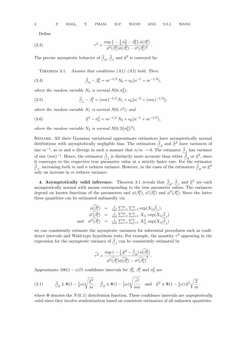
Define

(3.3) τ2 =exp

�− 1

2 σ20 − β0

0

�φ(β0

1)φ��(β0

1)φ(β01)− φ�(β0

1)2.

The precise asymptotic behavior of �β0, �β

1and �σ2 is conveyed by:

Theorem 3.1. Assume that conditions (A1)–(A5) hold. Then:

(3.4) �β0− β0

0 = m−1/2 N0 + op�n−1 + m−1/2),

where the random variable N0 is normal N(0,σ20);

(3.5) �β1− β0

1 = (mn)−1/2 N1 + op{n−2 + (mn)−1/2},

where the random variable N1 is normal N(0, τ2); and

(3.6) �σ2 − σ20 = m−1/2 N2 + op(n−1 + m−1/2),

where the random variable N2 is normal N(0, 2{σ20}2).

Remark. All three Gaussian variational approximate estimators have asymptotically normaldistibutions with asymptotically negligible bias. The estimators �β

0and �σ2 have variances of

size m−1, as m and n diverge in such a manner that n/m → 0. The estimator �β1

has varianceof size (mn)−1. Hence, the estimator �β

1is distinctly more accurate than either �β

0or �σ2, since

it converges to the respective true parameter value at a strictly faster rate. For the estimator�β

1, increasing both m and n reduces variance. However, in the cases of the estimators �β

0or �σ2

only an increase in m reduces variance.

4. Asymptotically valid inference. Theorem 3.1 reveals that �β0, �β

1and �σ2 are each

asymptotically normal with means corresponding to the true parameter values. The variancesdepend on known functions of the parameters and φ(β0

1), φ�(β01) and φ��(β0

1). Since the latterthree quantities can be estimated unbiasedly via

�φ(β01) = 1

mn

�mi=1

�nj=1 exp(Xij

�β1),

�φ�(β01) = 1

mn

�mi=1

�nj=1 Xij exp(Xij

�β1)

and �φ��(β01) = 1

mn

�mi=1

�nj=1 X2

ij exp(Xij�β

1)

we can consistently estimate the asymptotic variances for inferential procedures such as confi-dence intervals and Wald-type hypothesis tests. For example, the quantity τ2 appearing in theexpression for the asymptotic variance of �β

1can be consistently estimated by

�τ2 =exp

�− 1

2 �σ2 − �β0

� �φ(β01)

�φ��(β01) �φ(β0

1)− �φ�(β01)

2 .

Approximate 100(1− α)% confidence intervals for β00 , β0

1 and σ20 are

(4.1) �β0± Φ(1− 1

2α)

��σ2

m, �β

0± Φ(1− 1

2α)

��τ2

mnand �σ2 ± Φ(1− 1

2α) �σ2

�2m

.

where Φ denotes the N(0, 1) distribution function. These confidence intervals are asymptoticallyvalid since they involve studentization based on consistent estimators of all unknown quantities.


We ran a simulation study to evaluate the coverage properties of the Gaussian variational ap-proximate confidence intervals (4.1). The true parameter vector (β0

0 ,β01 ,σ2

0) was allowed to varyover {(−0.3, 0.2, 0.5), (2.2,−0.1, 0.16), (1.2, 0.4, 0.1), (0.02, 1.3, 1), (−0.3, 0.2, 0.1)} and the distri-bution of the Xij was taken to be either N(0, 1) or Uniform(−1, 1), the uniform distributionover the interval (−1, 1). The number groups m varied over 100, 200, . . . , 1000 with n fixed atm/10 throughout the study. For each of the ten possible combinations of true parameter vec-tor and Xij distribution, and sample size pairs, we generated 1000 samples and computed 95%confidence intervals based on (4.1).

Figure 4 shows the actual coverage percentages for the nominally 95% confidence intervals. Inthe case of β0

1 , the actual and nominal percentages are seen to have very good agreement — evenfor (m,n) = (100, 10). This is also the case for β0

0 for the first four true parameter vectors. Forthe fifth one, which has a relatively low amount of within-subject correlation, the asymptoticstake a bit longer to become apparent and we see that m ≥ 400 is required to get the actualcoverage above 90%, i.e. within 5% of the nominal level. For σ2

0, a similar comment applies, butwith m ≥ 800. The superior coverage of the β0

1 confidence intervals is in keeping with the fasterconvergence rate apparent from Theorem 3.1.

Lastly, we ran a smaller simulation study to check whether or not the lengths of the Gaussianvariational approximate confidence intervals are compromised in achieving the good coverageapparent in Figure 4. For each of the same settings used to produce that figure we generated100 samples and computed the exact likelihood-based confidence intervals using adaptive Gauss-Hermite quadrature (via the R language [12] package lme4 [1]). In almost every case, the Gaussianvariational approximate confidence intervals were slightly shorter than their exact counterparts.This reassuring result indicates that the good coverage performance is not accompanied by adecrease in precision.

value of m (n is fixed at m/10)

cove

rage

per

cent

age

85

90

95

( 00 = 0.3, 1

0 = 0.2, 02 = 0.5)

Xij ~ N(0, 1)

200 400 600 800 1000

( 00 = 2.2, 1

0 = 0.1, 02 = 0.16)

Xij ~ N(0, 1)

( 00 = 1.2, 1

0 = 0.4, 02 = 0.1)

Xij ~ N(0, 1)

200 400 600 800 1000

( 00 = 0.02, 1

0 = 1.3, 02 = 1)

Xij ~ N(0, 1)

( 00 = 0.3, 1

0 = 0.2, 02 = 0.1)

Xij ~ N(0, 1)

200 400 600 800 1000

( 00 = 0.3, 1

0 = 0.2, 02 = 0.5)

Xij ~ Uniform( 1, 1)

( 00 = 2.2, 1

0 = 0.1, 02 = 0.16)


200 400 600 800 1000

( 00 = 1.2, 1

0 = 0.4, 02 = 0.1)


( 00 = 0.02, 1

0 = 1.3, 02 = 1)


200 400 600 800 1000

85

90

95

( 00 = 0.3, 1

0 = 0.2, 02 = 0.1)


00

10

02


Table 1Definitions of the O(k) notation used in the proofs.

notation meaning

O(1) Op(m−1/2 + n

−1)O(2) Op(m

−1 + n−2)

O(3) O(nε−(1/2)), uniformly in 1 ≤ i ≤ m, for each ε > 0O(4) O(nε−1), uniformly in 1 ≤ i ≤ m, for each ε > 0O(5) O(nε−(3/2)), uniformly in 1 ≤ i ≤ m, for each ε > 0O(6) Op(m

−1 + nε−(3/2)), uniformly in 1 ≤ i ≤ m, for each ε > 0

O(7) Op{(m−1 + n−2) n

ε−(1/2)}, uniformly in 1 ≤ i ≤ m, for each ε > 0O(8) Op{(m−1/2 + n

−1)3 nε}, uniformly in 1 ≤ i ≤ m, for each ε > 0

O(9) Op{(mn)−1/2 + nε−(3/2)}, uniformly in 1 ≤ i ≤ m, for each ε > 0

O(10) Op{(m−1/2 + n−5/2) n

ε}, uniformly in 1 ≤ i ≤ m, for each ε > 0O(11) Op{(m−1/2

n−1 + n

−2) nε}, uniformly in 1 ≤ i ≤ m, for each ε > 0

5. Proof of Theorem 3.1. The proof Theorem 3.1 requires some additional notation, aswell as several stages of asymptotic approximation. This section provides full details, beginningwith definitions of the necessary notation.

5.1. Notation. Recall that β00 , β0

1 and σ20 denote the true values of parameters and that �β

0,

�β1

and �σ2 denote their respective Gaussian variational approximate estimators.The proofs use “O(k)” notation, for k = 1, . . . , 11, as defined in Table 1.

5.2. Formulae for estimators. First we give, in (5.1)–(5.5) below, the results of equating tozero the derivatives of �0(β, σ2)+�2(β, σ2,λ, µ) with respect to β0, β1, σ2, λi and µi, respectively:

m�

i=1

�Yi • −Bi exp

��µ

i+ 1

2�λ i

��= 0 ,(5.1)

m�

i=1

n�

j=1

Xij

�Yij − exp

� �β0+ �µ

i+ 1

2�λ i + �β

1Xij

� �= 0 ,(5.2)

1m

m�

i=1

��λ i + �µ2i

�= �σ2 ,(5.3)

�λ−1i −Bi exp

��µ

i+ 1

2�λ i

�− (�σ2)−1 = 0 , 1 ≤ i ≤ m,(5.4)

Yi • −Bi exp��µ

i+ 1

2�λ i

�− (�σ2)−1 �µ

i= 0 , 1 ≤ i ≤ m.(5.5)

These are the analogues of the likelihood equations in the conventional approach to inference.The next step is to put (5.1), (5.2) and (5.5) into more accessible form, in (5.6), (5.11) and

(5.12), respectively. Adding (5.5) over 1 ≤ i ≤ m and subtracting the result from (5.1) we deducethat

(5.6)m�

i=1

�µi= 0 .

Defining

∆ =1

mn

m�

i=1

n�

j=1

Xij�Yij − exp

�β0

0 + β01 Xij + Ui

��

we deduce that (5.2) is equivalent to:

∆ + exp�β0

0

� 1mn

m�

i=1

n�

j=1

Xij exp�Ui + β0

1 Xij�

− exp(β0)1

mn

m�

i=1

n�

j=1

Xij exp��µ

i+ 1

2�λ i + β1 Xij

�= 0 .(5.7)


Define ξi, ηi and ζi by, respectively,

1n

n�

j=1

Xij exp�β0

1 Xij�

= φ��β0

1

�exp(ξi) ,(5.8)

1n

n�

j=1

Xij exp� �β

1Xij

�= φ�(�β

1) exp

�ηi

�,(5.9)

exp� �β

0+ �µ

i+ 1

2�λ i

� 1n

n�

j=1

{exp(�β1Xij)− φ(�β

1)} = exp

�β0

0 + Ui�

×�φ�β0

1

�{1− exp(ζi)} +

1n

n�

j=1

�Yij exp

�− β0

0 − Ui�− φ

�β0

1

��− (�σ2n)−1 �µ

i.(5.10)

With probability converging to 1 as n → ∞ the definitions at (5.8)–(5.10) are valid simul-taneously for all 1 ≤ i ≤ m, because the variables ξi, ηi and ζi so defined converge to zero,uniformly in 1 ≤ i ≤ m, in probability. See (5.30), (5.31) and (5.25) below for approximationsto ξi, ηi and ζi; indeed, those formulae quickly imply that each of ξi, ηi and ζi equals O(3).

Without loss of generality, φ�(t) is bounded away from zero in a neighbourhood of β01 . Indeed,

if the latter property does not hold, simply add a constant to the random variable X to ensurethat φ�(β0

1) �= 0. We assume that β01 is in the just-mentioned neighbourhood, and we consider

only realizations for which β1 is also in the neighbourhood. (The latter property holds true withprobability converging to 1 as n →∞.) The definition of ζi at (5.10) can be justified using thefact that �µ

i< Yi •, as shown in Theorem 2 of [5].

In this notation we can write (5.7) as:

(5.11) ∆ + φ��β0

1

� 1m

m�

i=1

exp(β00 + Ui + ξi) = φ�(�β

1)

1m

m�

i=1

exp� �β

0+ �µ

i+ 1

2�λ i + ηi

�,

and write (5.5) as:

(5.12) exp� �β

0+ �µ

i+ 1

2�λ i

�φ(β1) = exp

�β0

0 + Ui + ζi�φ�β0

1

�.

Substituting (5.12) into (5.11) we obtain:

∆ exp�− β0

0

�φ�β0

1

�−1 + φ��β0

1

�φ�β0

1

�−1 1m

m�

i=1

exp(Ui + ξi)

= φ�(�β1) φ(�β

1)−1 1

m

m�

i=1

exp(Ui + ηi + ζi) .(5.13)

5.3. Approximate formulae for Ui and �λ i. The formulae are given at (5.16) and (5.18),respectively. To derive them, note that (5.5) implies that

(1 + O(3)) φ�β0

1

�exp

�β0

0 + Ui�− (1 + O(3)) φ

�β0

1

�exp

�β0

0 + �µi+ 1

2�λ i

�− (n�σ2)−1 �µ

i= 0 .

Here we have used the fact that, by [5],

(5.14) �β0− β0

0 = O(1) , �β1− β0

1 = O(1) ,

and that by (1.3), max1≤i≤m |Xi| = Op(nε) for all ε > 0. Therefore,

(5.15) (1 + O(3)) exp(Ui) = (1 + O(3)) exp��µ

i+ 1

2�λ i

�+ (cn�σ2)−1 �µ

i,


where c = φ(β01) exp(β0

0). The result max1≤i≤m |Ui| = Op{(log n)1/2} follows from properties ofextrema of Gaussian variables and the fact that m = O(nC) for a constant C > 0. Moreover, byTheorem 2 of [5], 0 < �λ i < �σ2. Therefore (5.15) implies that max1≤i≤n |�µ

i| = Op{(log n)1/2}.

(Note that, for any constant C > 0, exp{−C (log n)1/2} = n−C (log n)−1/2 , which is of larger orderthan n−ε for each ε > 0.) Hence, by (5.15),

(1 + O(3)) exp(Ui) = (1 + O(3)) exp��µ

i+ 1

2�λ i

�,

and so, taking logarithms,

(5.16) Ui = �µi+ 1

2�λ i + O(3) .

Formula (5.4) and property (5.14) entail:

(5.17) (n�λ i)−1 − (1 + O(3)) φ�β0

1

�exp

��µ

i+ 1

2�λ i + β0

0

�− (n�σ2)−1 = 0 .

Using (5.16) to substitute Ui + O(3) for �µi+ 1

2�λ i in (5.17) we deduce from that result that

(n�λ i)−1 = (1 + O(3)) φ�β0

1

�exp

�Ui + β0

0

�+ (n�σ2)−1

= (1 + O(3)) φ�β0

1

�exp

�Ui + β0

0

�,

where to obtain the second identity we again used the fact that

max1≤i≤m

|Ui| = Op{(log n)1/2}.

Therefore,

�λ i = (1 + O(3))�n φ

�β0

1

�exp

�Ui + β0

0

��−1

=�n φ

�β0

1

�exp

�Ui + β0

0

��−1 + O(5) ,(5.18)

where O(5) is as defined in Table 1. To obtain the second identity in (5.18) we used the fact thatmax1≤i≤m exp(−Ui) = O(nε) for all ε > 0.

5.4. Initial approximations to �β0− β0

0 and �β1− β0

1 . These approximations are given at(5.19), (5.21) and (5.29), and lead to central limit theorems for �β

1− β0

1 , �β0− β0

0 and �σ2 − σ20,

respectively. To derive the approximations, write γ(β1) = φ�(β1) φ(β1)−1 and note that, definingO(2) as in Table 1, we have:

γ(�β1) = γ(β0

1) +� �β

1− β0

1

�γ�

�β0

1

�+ Op

�� β1− β0

1

��2�

= γ�β0

1

�+

�1 + Op

�m−1/2 + n−1�� β

1− β0

1

�γ�(β0

1) .

(Here we have used (5.14).) Therefore, by (5.13) and for each ε > 0,

∆ exp�− β0

0

�φ�β0

1

�−1 + γ�β0

1

� 1m

m�

i=1

exp(Ui + ξi)

=�γ�β0

1

�+

�1 + Op

�m−1/2 + n−1�� β

1− β0

1

�γ�

�β0

1

��× 1

m

m�

i=1

exp(Ui + ηi + ζi) .

That is,

� �β1− β0

1

�γ�

�β0

1

� 1m

m�

i=1

exp(Ui + ηi + ζi)

= γ�β0

1

� 1m

m�

i=1

exp(Ui)�

exp(ξi)− exp�ηi + ζi

��+ ∆ exp

�− β0

0

�φ�β0

1

�−1 + O(2).(5.19)


Taking logarithms of both sides of (5.12) we obtain:

(5.20) log�φ(�β

1)�φ�β0

1

��= β0

0 − �β0+ Ui + ζi − �µ

i− 1

2�λ i ,

which, on adding over i and dividing by m, implies that

log�φ(�β

1)�φ�β0

1

��= β0

0 − �β0+

1m

m�

i=1

�Ui + ζi − �µ

i− 1

2�λ i

�,

which in turn gives

�β0− β0

0 = −� �β

1− β0

1

�γ�β0

1

�+

1m

m�

i=1

�Ui + ζi − �µ

i− 1

2�λ i

�+ O(2)

= −� �β

1− β0

1

�γ�β0

1

�+

1m

m�

i=1

(Ui + ζi)

−�2n φ

�β0

1

�exp

�β0

0 − 12 σ2

0

��−1 + O(6) ,(5.21)

where we used (5.18) to substitute for �λ i and (5.6) to eliminate �µifrom the right-hand side, and

employed (5.14) to bound (�β1−β0

1)2. Note too that E{exp(−Ui)} = exp(12 σ2

0); a term involvingE{exp(−Ui)} arises from

�i

�λ i via (5.18).

5.5. Approximation to ζi. The approximation is given at (5.25). First we derive an expansion,at (5.22) below, of �µ

i. Reflecting (5.16), define the random variable δi by �µ

i= Ui − 1

2�λ i + δi.

Then, by (5.16), δi = O(3). Define too B0ik =

�j Xk

ij exp(β00 + β0

1 Xij) for k = 0, 1, 2, and∆i = Yi • − B0

i0 exp(Ui); and let Fi denote the sigma-field generated by Ui and Xi1, . . . , Xin.Then E(∆i | Fi) = 0 and

Bi =�1 + �β

0− β0

0 + 12 (�β

0− β0

0)2�

B0i0 +

��β1− β0

1 +� �β

0− β0

0

� � �β1− β0

1

��B0

i1

+12

� �β1− β0

1

�2Bi2 + O(8) ,

uniformly in 1 ≤ i ≤ m for each ε > 0, where O(8) is as in Table 1. Therefore,

Yi • −Bi exp(Ui + δi) = Yi • −��

1 + �β0− β0

0 + 12 (�β

0− β0

0)2�

B0i0

+��β

1− β0

1 +� �β

0− β0

0

� � �β1− β0

1

��B0

i1 + 12

� �β1− β0

1

�2B0

i2

�

× exp(Ui)�1 + δi + 1

2 δ2i + O(5)

�+ n O(8) ,

where O(5) is as in Table 1. Therefore, defining

χi =��β

0− β0

0 + 12 (�β

0− β0

0)2�

B0i0 +

��β1− β0

1 +� �β

0− β0

0

� � �β1− β0

1

��B0

i1

+12

� �β1− β0

1

�2B0

i2 ,

we see that the left-hand side of (5.5) equals:

Yi • −Bi exp(Ui + δi)− (�σ2)−1 �µi

= ∆i −B0i0 exp(Ui)

�δi + 1

2 δ2i + O(5)

�− χi exp(Ui)

�1 + δi + 1

2 δ2i + O(5)

�

−(�σ2)−1 �Ui − 1

2�λ i + δi

�+ n O(8)

= ∆i −�χi exp(Ui) + (�σ2)−1 �

Ui − 12

�λ i

��− δi

��B0

i0 + χi�

exp(Ui) + (�σ2)−1�

12 δ2

i

�B0

i0 + χi�

exp(Ui) + n O(5) + n O(8) .


Hence, (5.5) implies that:

δi + 12 δ2

i(B0

i0 + χi) exp(Ui)(B0

i0 + χi) exp(Ui) + (�σ2)−1=

∆i − χi exp(Ui)− (�σ2)−1 (Ui − 12

�λ i)(B0

i0 + χi) exp(Ui) + (�σ2)−1+ O(5) + O(8) ,

which implies that:

δi =∆i − χi exp(Ui)

(B0i0 + χi) exp(Ui)

+ O(4) =�n exp

�β0

0

�φ�β0

1

��−1 {∆i exp(−Ui)− χi} + O(4)

=�n exp

�β0

0

�φ�β0

1

��−1 ∆i exp(−Ui)−� �β

0− β0

0

�−

� �β1− β0

1

�γ�β0

1

�+ O(4) .

Here we have defined O(4) is as in Table 1 and have used the fact that n−1 B0i0 = exp(β0

0) φ(β01)+

O(3) andn−1 B0

i1 = exp�β0

0

�φ�

�β0

1

�+ O(3) = exp

�β0

0

�φ�β0

1

�γ�β0

1

�+ O(3) .

Therefore,

�µi

= Ui − 12

�λ i + δi

= Ui +�n exp

�β0

0

�φ�β0

1

��−1 ∆i exp(−Ui)−� �β

0− β0

0

�−

� �β1− β0

1

�γ�β0

1

�+ O(4)

= Ui − U +�n exp

�β0

0

�φ�β0

1

��−1 ∆i exp(−Ui) + O(4) ,(5.22)

where to obtain the second identity we used (5.18) to place �λ i into the remainder, and to obtainthe third identity we used (5.21) to show that �β

0− β0

0 + (�β1− β0

1) γ�(β01) = U + O(4). Here we

have used the property, deducible from (5.10), (5.16) and (5.18), that ζi = O(3) and ζ = O(4).The next step is to substitute the right-hand side of (5.22) for �µ

i, and the right-hand side of

(5.18) for �λ i, in (5.10), and derive an expansion, at (5.25) below, of ζi. We obtain:

�1 +

�n exp

�β0

0

�φ�β0

1

��−1 ∆i exp(−Ui)− U� 1

n

n�

j=1


1)}

= −φ�β0

1

� �ζi + 1

2 ζ2i

�+

1n

n�

j=1

�Yij exp

�− β0

0 − Ui�− φ

�β0

1

��

− exp�− β0

0 − Ui�(�σ2n)−1 Ui + O(5) ,

whence

φ�β0

1

� �ζi + 1

2 ζ2i

�

=1n

n�

j=1

�Yij exp

�− β0

0 − Ui�− φ

�β0

1

��− 1

n

n�

j=1


1)}

−��

n exp�β0

0

�φ�β0

1

��−1 ∆i exp(−Ui)− U� 1

n

n�

j=1

�exp

� �β1Xij

�− φ

� �β1

�}

− exp�− β0

0 − Ui�(�σ2n)−1 Ui + O(5) .(5.23)

However, defining

(5.24) Dik(b) =1n

n�

j=1

�Xk

ij exp(b Xij)− φ(k)(b)�

= O(3)


for k = 0, 1, 2, and ∆i = Yi • −B0i0 exp(Ui), we see that

n�

j=1

�Yij exp

�− β0

0 − Ui�− φ

�β0

1

��−

n�

j=1


1)}

=n�

j=1

�Yij exp

�− β0

0 − Ui�− φ

�β0

1

��

−n�Di0

�β0

1

�+

� �β1− β0

1

�Di1

�β0

1

��+ O(3)

= ∆i exp�− β0

0 − Ui�− n

� �β1− β0

1

�Di1

�β0

1

�+ O(3) ,

and so, by (5.23),

φ�β0

1

� �ζi + 1

2 ζ2i

�= n−1 exp

�− β0

0 − Ui� �

∆i�1− φ

�β0

1

�−1Di0

�β0

1

��− (�σ2)−1 Ui

�

−� �β

1− β0

1

�Di1

�β0

1

�+ U Di0

�β0

1

�+ O(5) .

Therefore,

φ�β0

1

�ζi = n−1 exp

�− β0

0 − Ui� �

∆i�1− φ

�β0

1

�−1Di0

�β0

1

��− (�σ2)−1 Ui

�

−� �β

1− β0

1

�Di1

�β0

1

�+ U Di0

�β0

1

�

−12 φ

�β0

1

�−1 �n−1 exp

�− β0

0 − Ui�∆i

�2 + O(5)(5.25)

Result (5.25), and the fact that n/m→ 0 as n→∞, imply that

φ(β01)

1m

m�

i=1

Uiζi = − 1mn

exp(−β00)

(σ2)0m�

i=1

U2i exp(−Ui)

− 12m

φ(β01)−1

m�

i=1

Ui

�n−1 exp(−β0

0 − Ui)∆i

�2+ op(n−1)

= − 1n

exp�1

2(σ2)0 − β00

��1 + 1

2(σ2)0�+ op(n−1)(5.26)

Here we have used the fact that E{U2i exp(−Ui)} = exp(1

2 σ20) σ2

0 (1 + σ20).

5.6. Initial approximation to σ2 − σ20. Starting from (5.20); using (5.21) to substitute for

�β0− β0

0 ; using (5.18) to substitute for �λ i; and defining U = m−1 �i Ui and ζ = m−1 �

i ζi; weobtain:

�µi

= Ui + ζi − 12

�λ i − log�φ(�β

1)�φ�β0

1

��−

� �β0− β0

0

�

= Ui + ζi − 12

�λ i −� �β

1− β0

1

�γ�β0

1

�−

� �β0− β0

0

�+ O(2)

= Ui + ζi −�2n φ

�β0

1

�exp

�Ui + β0

0

��−1 − (U + ζ)

+�2n φ

�β0

1

�exp

�β0

0 − 12 σ2

0

��−1 + O(6) .(5.27)

Hence, squaring both sides of (5.27) and adding,

1m

m�

i=1

�µ2i

=1m

m�

i=1

(Ui + ζi − U − ζ)2

−{mnφ(β01) exp(β0

0)}−1m�

i=1

exp(−Ui)(Ui + ζi − U − ζ) + O(6) .(5.28)

Combining (5.3), (5.18), (5.25) and (5.28) we deduce that:

�σ2 =1m

m�

i=1

��λ i + �µ2i

�= σ2

0 +1m

m�

i=1

�(Ui + ζi − U − ζ)2 − σ2

0

�

+�n φ

�β0

1

�exp

�β0

0 − 12 σ2

0

��−1 �1 + σ2

0

�+ O(6) .(5.29)


5.7. Approximations to ξi and ηi. The approximations are given at (5.30) and (5.31), re-spectively, and are derived as follows. Note the definition of Dik(b) at (5.24). In that notation,observing that n/m → 0 and recalling (5.14), it can be deduced from (5.8) and (5.9) that,uniformly in 1 ≤ i ≤ m,

(5.30) ξi = φ��β0

1

�−1Di1

�β0

1

�− 1

2

�φ�

�β0

1

�−1Di1

�β0

1

��2 + O(5) ,

ηi = φ��β0

1

�−1�Di1

�β0

1

�+

� �β1− β0

1

� �Di2

�β0

1

�− φ�

�β0

1

�−1φ��

�β0

1

�Di1

�β0

1

��

−12

�φ�

�β0

1

�−1Di1

�β0

1

��2 + O(5) .(5.31)

Result (5.30) is derived by writing (5.8) as:

(5.32) φ��β0

1

�−1Di1

�β0

1

�= exp(ξi)− 1 = ξi + 1

2 ξ2i + Op

�|ξi|3

�,

and then inverting the expansion. (The result max1≤i≤m |ξi| = op(1), in fact O(3), used in thisargument, is readily derived.) To obtain (5.31), note that the analogue of (5.32) in that case is:

(5.33) φ�(�β1)−1 Di1(�β

1) = exp(ηi)− 1 = ηi + 1

2 η2i + Op

�|ηi|3

�,

and that, uniformly in 1 ≤ i ≤ m,

φ�(�β1)−1 Di1(�β

1) =

�φ�

�β0

1

�+

� �β1− β0

1

�φ��

�β0

1

�+ O(2)

�−1

×�Di1

�β0

1

�+

� �β1− β0

1

�Di2

�β0

1

�+ O(7)

�

= φ��β0

1

�−1�1−

� �β1− β0

1

�φ�

�β0

1

�−1φ��

�β0

1

��

×�Di1

�β0

1

�+

� �β1− β0

1

�Di2

�β0

1

��+ O(7)

= φ��β0

1

�−1�Di1

�β0

1

�+

� �β1− β0

1

� �Di2

�β0

1

�

−φ��β0

1

�−1φ��

�β0

1

�Di1

�β0

1

��+ O(7) .(5.34)

Result (5.31) follows from (5.33) and (5.34) on inverting the expansion at (5.33).

5.8. Another approximation to �β1− β0

1 , and final approximations to �β0− β0

0 and σ2 − σ20.

Next we use the expansions (5.30), (5.31) and (5.25) of ξi, ηi and ζi to refine the approximationsderived in section 2.3. The results are given in (5.40), (5.41) and (5.45) in the cases of �β

0− β0

0 ,�β

1− β0

1 and σ2 − σ20, respectively.

It can be deduced from (5.31) and (5.25) that

(5.35)1m

m�

i=1

exp(Ui + ηi + ζi) = exp�1

2 σ20

�+ O(3) .

By (5.30), (5.31) and (5.25),

1m

m�

i=1

exp(Ui)�


��

=1m

m�

i=1

exp(Ui)�ξi − ηi − ζi + 1

2

�ξ2i − (ηi + ζi)2

��+ O(5)

= − 1m

m�

i=1

exp(Ui)�ζi + 1

2

�2 ηi ζi + ζ2

i

��+ O(5) + Op

�� β1− β0

1

�� nε−(1/2)�.(5.36)


Defining O(9) as at Table 1 we deduce from (5.25) that

1m

m�

i=1

exp(Ui) ζi = −12 φ

�β0

1

�−2 1mn2

m�

i=1

exp�− 2 β0

0 − Ui�∆2

i

+Op�(mn)−1/2� + O(5)

= −(2n)−1 φ�β0

1

�−1 exp�− β0

0

�+ O(9) ,(5.37)

where we have used the fact that n/m → 0 and, since Yi •, conditional on Fi, has a Poissondistribution with mean B0

i0 exp(Ui), then

E�

exp(−Ui) ∆2i

�= E

�exp(−Ui) {Yi • − E(Yi • | Fi)}2� = E{exp(−Ui) var(Yi • | Fi)}

= E�

exp(−Ui) B0i0 exp(Ui)

�= E

�B0

i0

�= n exp

�β0

0

�φ�β0

1

�.

1m

m�

i=1

exp(Ui) ζ2i = φ

�β0

1

�−2 1mn2

m�

i=1

exp�− 2 β0

0 − Ui�∆2

i + O(9)

= n−1 φ�β0

1

�−1 exp�− β0

0

�+ O(9) .

Moreover, since by (5.31) and (5.25),

ηi = φ��β0

1

�−1Di1

�β0

1

�+ O(4) , ζi = φ

�β0

1

�−1n−1 exp

�− β0

0 − Ui�∆i + O(4) ,

and for k ≥ 0,

E�

exp(Ui) Dik�β0

1

�exp

�− Ui

�∆i

�= E

�Dik

�β0

1

�E(∆i | Fi)

�= 0 ,

then

(5.38)1m

m�

i=1

exp(Ui) ηi ζi = O(5) .

Together, (5.36), (5.37), (5.38) and (5.38) imply that

1m

m�

i=1

exp(Ui)�


��

= (2n)−1 φ�β0

1

�−1 exp�− β0

0

�− (2n)−1 φ

�β0

1

�−1 exp�− β0

0

�

+O(9) + Op�� β

1− β0

1

�� nε−(1/2)�

= O(9) + Op�� β

1− β0

1

�� nε−(1/2)� .(5.39)

Combining (5.19), (5.35) and (5.39), and noting that ∆ = Op{(mn)−1/2} and n/m → 0, wededuce that:

(5.40) �β1− β0

1 = O(9) .

Together, (5.21) and (5.40) imply that

(5.41) �β0− β0

0 = U + ζ − c0 n−1 + op�m−1/2 + n−1� ,

wherec0 =

�2 φ

�β0

1

�exp

�β0

0 − 12 σ2

0

��−1.


Result (3.4) Theorem 3.1 is a direct consequence of (5.41) and the property:

ζ = − 1m

m�

i=1

Ui�n(σ2)0 exp(Ui + β0

0)φ(β01)

�−1

−12φ(β0

1)−2E�n−1 exp(−β0

0 − Ui)∆i�2 + op(n−1)

= c0n−1 + op(n−1).(5.42)

Results (5.25) and (5.40), and the property

E�

exp(−2 Ui) ∆2i

�= E

�B0

i0 exp(−Ui)�

= n exp�β0

0 + 12 σ2

0

�φ�β0

1

�,

imply that

1m

m�

i=1

ζ2i = φ

�β0

1

�−2 1mn2

m�

i=1

exp�− 2 β0

0 − 2 Ui�∆2

i + op(1)

= n−1 φ�β0

1

�−1 exp�1

2 σ20 − β0

0

�+ op

�n−1� = 2 c0 n−1 + op

�n−1� .(5.43)

By (5.26),

(5.44)1m

m�

i=1

Ui ζi = − 1n

φ�β0

1

�−1 exp�1

2 σ20 − β0

0

� �1 + 1

2σ20

�+ op

�n−1� .

Together, (5.42)–(5.44) give:

1m

m�

i=1

�(Ui + ζi − U − ζ)2 − (σ2)0

�

=1m

m�

i=1

(U2i − (σ2)0) +

1m

m�

i=1

ζ2i − ζ2 +

2m

m�

i=1

Uiζi − 2U ζ + Op(m−1)

=1m

m�

i=1

(U2i − (σ2)0) + 2n−1c0 − 2n−1c0(2 + (σ2)0) + op(m−1/2 + n−1)

=1m

m�

i=1

(U2i − (σ2)0)− 2n−1c0(1 + σ2

0) + op(m−1/2 + n−1)

Hence, by (5.29),

(5.45) �σ2 − σ20 =

1m

m�

i=1

�U2

i − σ20

�+ op

�m−1/2 + n−1� .

Result (3.6) of Theorem 3.1 is a direct consequence of (5.45).

5.9. Final approximation to �β1− β0

1 . Our first step is to sharpen the expansion of (5.5)at (5.15); see (5.49), which leads to (5.54), the principal analogue of (5.15).

Recall that

(5.46) ∆i = Yi • − exp�β0

0 + Ui� n�

j=1

exp(β01 Xij) = Yi • − exp(Ui) B0

i0 .


Also, in view of (5.40) and (5.41),

Bi = exp� �β

0

� n�

j=1

exp(�β1Xij)

= exp�β0

0

� �1 +

� �β0− β0

0

�+ 1

2 (�β0− β0

0)2 + 16

� �β0− β0

0

�3�

×n�

j=1

�1 +

� �β1− β0

1

�Xij + 1

2

� �β1− β0

1

�2X2

ij

�

× exp�β0

1 Xij�+ Op

�m−2 n + m−3/2 n−1/2 + m−1 + nε−3�

= exp�β0

0

� n�

j=1

�1 +

� �β0− β0

0

�+ 1

2

� �β0− β0

0

�2 + 16

� �β0− β0

0

�3

+� �β

1− β0

1

�Xij + 1

2

� �β1− β0

1

�2X2

ij +� �β

0− β0

0

� � �β1− β0

1

�Xij

�exp

�β0

1 Xij�

+Op�m−1/2 nε + nε−(5/2)�

=�1 +

� �β0− β0

0

�+ 1

2

� �β0− β0

0

�2 + 16

� �β0− β0

0

�3�

B0i0

+�1 +

� �β0− β0

0

�� β1− β0

1

�B0

i1 + 12

� �β1− β0

1

�2B0

i2 + O(10) ,

where O(10) is defined in Table 1. Hence, recalling that δi = �µi+ 1

2�λ i−Ui, we see that, for each

ε > 0, we have, uniformly in 1 ≤ i ≤ n,

Yi • −Bi exp(δi + Ui) = Yi • −B0i0 exp(δi + Ui)

−��β

0− β0

0

�+ 1

2

� �β0− β0

0

�2 + 16

� �β0− β0

0

�3�

B0i0

+�1 +

� �β0− β0

0

�� β1− β0

1

�B0

i1 + 12

� �β1− β0

1

�2B0

i2

�exp(δi + Ui) + O(10) .(5.47)

Combining (5.46) and (5.47) we obtain:

Yi • −Bi exp(δi + Ui) = ∆i − exp(Ui)�{exp(δi)− 1}B0

i0

+��β

0− β0

0

�+ 1

2

� �β0− β0

0

�2 + 16

� �β0− β0

0

�3�

B0i0

+�1 +

� �β0− β0

0

�� β1− β0

1

�B0

i1 + 12

� �β1− β0

1

�2B0

i2

�exp(δi)

�+ O(10) .

Therefore, (5.5) implies that:

(�σ2)−1 �µi

= ∆i − exp(Ui)�{exp(δi)− 1}B0

i0

+��β

0− β0

0

�+ 1

2

� �β0− β0

0

�2 + 16

� �β0− β0

0

�3�

B0i0

+�1 +

� �β0− β0

0

�� β1− β0

1

�B0

i1 + 12

� �β1− β0

1

�2B0

i2

�exp(δi)

�+ O(10) ,

or equivalently,

exp(Ui)�{exp(δi)− 1}B0

i0

+exp(δi)��β

0− β0

0

�+ 1

2

� �β0− β0

0

�2 + 16

� �β0− β0

0

�3�

B0i0

+�1 +

� �β0− β0

0

�� β1− β0

1

�B0

i1 + 12

� �β1− β0

1

�2B0

i2

��+ (�σ2)−1 �

δi + Ui − 12

�λ i

�

= ∆i + O(10) .(5.48)


Substituting the far right-hand side of (5.18) for �λ i in (5.48) we deduce that:

exp(δi)− 1 + exp(δi)��β

0− β0

0

�+ 1

2

� �β0− β0

0

�2 +� �β

1− β0

1

� �B0

i1

�B0

i0

��

+��σ2 B0

i0 exp(Ui)�−1 �

δi + Ui)

=�B0

i0 exp(Ui)�−1 ∆i + O(11) ,(5.49)

where O(11) is as defined in Table 1. Result (5.49) implies that

(5.50) δi + 12 δ2

i Gi2 + 16 δ3

i Gi3 = Gi + O(11) ,

where, putting

(5.51) Gi1 = 1 +� �β

0− β0

0

�+ 1

2

� �β0− β0

0

�2 +� �β

1− β0

1

� �Bi1

�B0

i0

�+

��σ2 B0

i0 exp(Ui)�−1

,

we define Gi, Gi2 and Gi3 by Gi3 Gi1 = 1,

(5.52) Gi2 Gi1 = 1 +� �β

0− β0

0

�+

� �β1− β0

1

� �Bi1

�B0

i0

�,

Gi Gi1 =�B0

i0 exp(Ui)�−1 ∆i −

��σ2 B0

i0 exp(Ui)�−1

Ui

−��β

0− β0

0

�+ 1

2

� �β0− β0

0

�2 +� �β

1− β0

1

� �B0

i1

�B0

i0

��.(5.53)

Solving (5.50) for δi we deduce that, for each ε > 0,

(5.54) δi = Gi − 12 Gi2 G2

i −�1

6 Gi3 − 12 G2

i2

�G3

i + O(11) ,

uniformly in 1 ≤ i ≤ n. Now, Gi1, Gi2 and Gi3 each equal 1 + Op(m−1/2 + nε−1). Therefore,16 Gi3 − 1

2 G2i2 = −1

3 + Op(m−1/2 + nε−1). Using (5.51), (5.52) and (5.53) we deduce that

Gi2 = 1−��σ2 B0

i0 exp(Ui)�−1 + Op

�m−1 + nε−2� , Gi = Hi + O(11) ,

where

Hi =��

B0i0 exp(Ui)

�−1 ∆i −��σ2 B0

i0 exp(Ui)�−1

Ui

−��β

0− β0

0

�+ 1

2

� �β0− β0

0

�2 +� �β

1− β0

1

� �B0

i1

�B0

i0

��

×�1−

� �β0− β0

0

�−

� �β1− β0

1

� �Bi1

�B0

i0

�−

��σ2 B0

i0 exp(Ui)�−1

�.

Note too that Gi2 H2i = H2

i + Op(m−1/2 nε−1 + nε−2). Combining the results from (5.54) downwe see that

(5.55) δi = Hi − 12 H2

i + 13 H3

i + O(11) .

Note that, as a → 0, exp(a− 12 a2 + 1

3 a3)− 1 = a + O(a4) as a → 0. This property, (5.55) andthe fact that H4

i = Op(nε−2) imply that

(5.56) exp(δi)− 1 = Hi + O(11) .

The formula immediately preceding (5.19) is equivalent to:

�1 + Op

�m−1/2 + n−1�� γ�

�β0

1

� � �β1− β0

1

� 1m

m�

i=1

exp(Ui + ηi + ζi)

= ∆ exp�− β0

0

�φ�β0

1

�−1 + γ�β0

1

� 1m

m�

i=1

{exp(ξi)− exp(ηi + ζi)} exp(Ui) .(5.57)


Since ηi and ζi both equal O(3) (see (5.25) and (5.31)), and m−1 �mi=1 exp(Ui) = E{exp(U1)}+

op(1) = exp{σ20/2} + op(1), then (5.57) implies that

{1 + op(1)} γ��β0

1

� � �β1− β0

1

�exp{σ2

0/2}

= ∆ exp�− β0

0

�φ�β0

1

�−1 + γ�β0

1

� 1m

m�

i=1

{exp(ξi)− exp(ηi + ζi)} exp(Ui) .(5.58)

Formulae (5.8) and (5.9) are together equivalent to:

φ��β0

1

�{exp(ξi)− 1} =

1n

n�

j=1

{Xij exp�β0

1 Xij�− φ�

�β0

1

��,(5.59)

φ�(�β1) {exp(ηi)− 1} =

1n

n�

j=1

�Xij exp(�β

1Xij)− φ�(�β

1)�

.(5.60)

Result (5.60) implies that, for each ε > 0,�φ�

�β0

1

�+ Op

�� β1− β0

1

�� {exp(ηi)− 1}

=1n

n�

j=1

�Xij exp

�β0

1 Xij�− φ�

�β0

1

��+ Op

�� β1− β0

1

�� nε−(1/2)� ,

uniformly in 1 ≤ i ≤ n. Therefore, since ηi = O(3) (see (5.31)), then

φ��β0

1

�{exp(ηi)− 1} =

1n

n�

j=1

�Xij exp

�β0

1 Xij�− φ�

�β0

1

��+ Op

�� β1− β0

1

�� nε−(1/2)�,

which in company with (5.60) implies that

φ��β0

1

�{exp(ηi)− exp(ξi)} = Op

�� β1− β0

1

�� nε−(1/2)� ,

uniformly in 1 ≤ i ≤ n. Hence, since ηi = O(3) and ζi = O(3) (see (5.25) and (5.31)),

exp(ξi)− exp(ηi + ζi) = {exp(ξi)− exp(ηi)} exp(ζi) + exp(ξi) {1− exp(ζi)}= exp(ξi) {1− exp(ζi)} + Op

�� β1− β0

1

�� nε−(1/2)� ,(5.61)

uniformly in i. Combining (5.58) and (5.61) we deduce that

{1 + op(1)} γ��β0

1

� � �β1− β0

1

�exp{1

2σ20}

= ∆ exp�− β0

0

�φ�β0

1

�−1 + γ�β0

1

� 1m

m�

i=1

exp(ξi + Ui) {1− exp(ζi)} .(5.62)

Next we return to (5.10), which we write equivalently as

φ�β0

1

�{1− exp(ζi)} = exp

� �β0− β0

0 + δi� 1

n

n�

j=1


1)}

− 1n

n�

j=1

�Yij exp

�− β0

0 − Ui�− φ

�β0

1

��+ (�σ2n)−1 �µ

iexp

�− β0

0 − Ui�.(5.63)

So that we might replace �β1

by β01 on the right-hand side of (5.63) we observe that


1n

n�

j=1


1)}

=1n

n�

j=1

�exp

�β0

1 Xij�− φ

�β0

1

��+ Op

�� β1− β0

1

�� nε−(1/2)� .(5.64)

Combining (5.62)–(5.64) we obtain:

{1 + op(1)} γ��β0

1

� � �β1− β0

1

�exp{1

2σ20}

= ∆ exp�− β0

0

�φ�β0

1

�−1

+φ�

�β0

1

�

φ�β0

1

�2

1m

m�

i=1

exp(ξi + Ui)�exp

� �β0− β0

0 + δi� 1

n

n�

j=1

�exp

�β0

1 Xij�− φ

�β0

1

��

− 1n

n�

j=1

�Yij exp

�− β0

0 − Ui�− φ

�β0

1

��+ (�σ2n)−1 �µ

iexp

�− β0

0 − Ui��

.(5.65)

(Recall that γ = φ�φ−1, and so γ/φ = φ�φ−2.)Since exp(ξi)− 1 = Di1(β0

1) φ�(β01)−1 (see (5.8)) and �β

0− β0

0 = Op(m−1/2 + n−1) (see (5.41))then

1m

m�

i=1

exp(ξi + Ui) exp� �β

0− β0

0 + δi� 1

n

n�

j=1

�exp

�β0

1 Xij�− φ

�β0

1

��

=�1 +

� �β0− β0

0

�+ 1

2

� �β0− β0

0

�2� 1

m

m�

i=1

exp(ξi + δi + Ui) Di0�β0

1

�

+Op�m−3/2 + n−3�

=�1 +

� �β0− β0

0

�+ 1

2

� �β0− β0

0

�2�

× 1m

m�

i=1

exp(δi + Ui)�1 + Di1

�β0

1

�φ�

�β0

1

�−1�

Di0�β0

1

�

+Op�m−3/2 + n−3�.(5.66)

Likewise,

1m

m�

i=1

exp(ξi + Ui)1n

n�

j=1

�Yij exp

�− β0

0 − Ui�− φ

�β0

1

��

=1m

m�

i=1

exp(Ui)�1 + Di1

�β0

1

�φ�

�β0

1

�−1��

n−1 ∆i exp�− β0

0 − Ui�+ Di0

�β0

1

��,(5.67)

and, since�

i �µi= 0 (see (5.6)),

1m

m�

i=1

exp(ξi + Ui) (�σ2n)−1 �µiexp

�− β0

0 − Ui�

=1

�σ2 mn

m�

i=1

exp�ξi − β0

0

��µ

i

= exp�− β0

0

� 1�σ2 mn

m�

i=1

�1 + Di1

�β0

1

�φ�

�β0

1

�−1�

�µi

= exp�− β0

0

�φ�

�β0

1

�−1 1�σ2 mn

m�

i=1

Di1�β0

1

��µ

i= Op

�m−1/2 n−3/2� .(5.68)


Combining (5.65)–(5.68) we see that

{1 + op(1)} γ��β0

1

� � �β1− β0

1

�exp{1

2σ20}

= ∆ exp�− β0

0

�φ�β0

1

�−1 +φ�

�β0

1

�

φ�β0

1

�2

��1 +

� �β0− β0

0

�+ 1

2

� �β0− β0

0

�2�

× 1m

m�

i=1

exp(δi + Ui)�1 + Di1

�β0

1

�φ�

�β0

1

�−1�

Di0�β0

1

�

− exp�− β0

0

� 1m

m�

i=1

�1 + Di1

�β0

1

�φ�

�β0

1

�−1�

×�n−1 ∆i + exp

�β0

0 + Ui�Di0

�β0

1

��

+Op�m−1/2 n−1 + n−3� .(5.69)

Using the fact that E(∆i | Fi) = 0 and Di1(β01) = O(3) it can be proved that, for all ε > 0,

1mn

m�

i=1

exp�− β0

0

� �1 + Di1

�β0

1

�φ�

�β0

1

�−1�

∆i

= exp�− β0

0

� 1mn

m�

i=1

∆i + Op�m−1/2 n−1� .(5.70)

Also,

∆� ≡ ∆ exp�− β0

0

�φ�β0

1

�−1 −exp

�− β0

0

�φ�(β0

1)φ(β0

1)21

mn

m�

i=1

∆i

= φ�β0

1

�−1 exp�− β0

0

� 1mn

m�

i=1

n�

j=1

�Xij −

φ��β0

1

�

φ�β0

1

��

Yij − exp�β0

0 + β01 Xij + Ui

��.(5.71)

Moreover, using (5.41) and the fact that Di0(β01) = O(3) and E{Di0(β0

1) |Ui} = 0, it can beshown that

� �β0− β0

0

� 1m

m�

i=1

exp(Ui)�1 + Di1

�β0

1

�φ�

�β0

1

�−1�

Di0�β0

1

�

= Op

��m−1/2 + n−1� ·

�m−1/2 nε−(1/2)��

= Op�m−1/2 nε−1� .(5.72)

Combining (5.69)–(5.72) we deduce that

{1 + op(1)} γ��β0

1

� � �β1− β0

1

�exp{1

2σ20}

= ∆� +φ�

�β0

1

�

φ�β0

1

�2

1m

m�

i=1

exp(Ui) {exp(δi)− 1}�1 + Di1

�β0

1

�φ�

�β0

1

�−1�

Di0�β0

1

�

+Op�m−1/2 nε−1 + n−3� .(5.73)

Using (5.56) to substitute for exp(δi)−1 in (5.73), and noting that Dik(β01) = O(3) for k = 0, 1,

we deduce from (5.73) that

{1 + op(1)} γ��β0

1

� � �β1− β0

1

�exp{1

2σ20}

= ∆� +φ�

�β0

1

�

φ�β0

1

�2 ψ(H) + Op�m−1/2 nε−1 + nε−(5/2)� ,(5.74)


where H = (H1, . . . ,Hm), Hi is as defined at (5.55), and, given a sequence of random variablesK = (K1, . . . ,Km), we put

ψ(K) =1m

m�

i=1

exp(Ui) Ki

�1 + Di1

�β0

1

�φ�

�β0

1

�−1�

Di0�β0

1

�.

Note again that |Di0(β01)| = O(3), and the dominant term on the right-hand side of formula (5.55)

for Hi is {B0i0 exp(Ui)}−1 ∆i. Moreover, |�β

0− β0

0 | = Op(m−1/2 + n−1) (see (5.41)), |�β1− β0

1 | =Op{(mn)−1/2 + nε−(3/2)} (see (5.41)),

��σ2 B0

i0 exp(Ui)�−1 =

�n σ2

0 φ�β0

1

�exp

�β0

0 + Ui��−1 + Op

�nε−(3/2)� ,

B0i1 B0

i0−1 = φ�

�β0

1

�φ�β0

1

�−1 + O(3) .

Combining these properties we deduce that

(5.75)(5.74) continues to hold if, on the right-hand side, ψ(H) is replacedby ψ(H �) where H � = (H �

1, . . . ,H�m) and H �

i = H(1)i −H(2)

i −H(3)i ,

with

H(1)i =

�B0

i0 exp(Ui)�−1 ∆i

�1−

� �β0− β0

0

�−

�n σ2

0 φ�β0

1

�exp(Ui)

�−1�,

H(2)i = {�σ2 B0

i0 exp(Ui)}−1 Ui

and H(3)i =

� �β0− β0

0

�+ 1

2

� �β0− β0

0

�2 +� �β

1− β0

1

� �φ�

�β0

1

��φ�

�β0

1

��.

(Note that H(3)i does not depend on i.) It can be proved from the properties E(∆i | Fi) = 0 and

|Di0(β01)| = O(3) that, with H(j) denoting (H(j)

1 , . . . ,H(j)m ), we have:

(5.76) ψ�H(1)� = Op

�m−1/2 n−1� .

More simply, since E(Ui |Xi1, . . . , Xin) = 0 then

ψ�H(2)� =

1m

m�

i=1

��σ2 B0

i0

�−1Ui

�1 + Di1

�β0

1

�φ�

�β0

1

�−1�

Di0�β0

1

�

= Op�m−1/2 n−3/2� .

Furthermore, writing 1 = (1, . . . , 1), an n-vector; and noting that the properties E{Dik(β01) |Ui} =

0, var{Dik(β01) |Ui} = O(n−1) and E{exp(Ui)} = exp

�12 σ2

0

�imply that

ψ(1) =1m

m�

i=1

exp(Ui)�1 + Di1

�β0

1

�φ�

�β0

1

�−1�

Di0�β0

1

�

= φ��β0

1

�−1 1m

m�

i=1

exp(Ui) Di1�β0

1

�Di0

�β0

1

�+ Op

�m−1/2 n−1/2�

= n−1 {φ��2β0

1

�φ�

�β0

1

�−1 − φ�β0

1

�} exp

�12 σ2

0

�+ Op

�m−1/2 n−1/2 + n−3/2� ;

we obtain:

ψ�H(3)� =

��β0− β0

0

�+ 1

2

� �β0− β0

0

�2 +� �β

1− β0

1

� �φ�

�β0

1

��φ�

�β0

1

��ψ(1)

=� 1

n

�φ�(2β0

1)φ�(β0

1)−1 − φ(β01)

�exp(1

2(σ2)0) + Op(m−1/2n−1/2 + n−3/2)�

×�(�β

0− β0

0) +12(�β

0− β0

0)2 + (�β1− β0

1){φ�(β01)/φ(β0

1)}�

= Op(m−1/2n−1)


To obtain the last line here we used (3.4) of Theorem 3.1, already proved in Section 5.8 above.Combining (5.74)–(5.77), and noting that the function ψ is linear, so that

ψ(H) = ψ(H(1))− ψ(H(2))− ψ(H(3)),

we deduce that

{1 + op(1)} γ��β0

1

� � �β1− β0

1

�exp(1

2σ20) = ∆� + op

�(mn)−1/2 + n−2� .

Furthermore, the random variable ∆�, defined at (5.71), is asymptotically normally distributedwith zero mean and variance

1mn

exp(−2 β00

�E

��X11 −

φ�(β01)

φ(β01)

�2E

�E

�Y11 − E(Y11 |X11, U1)

�2�� X11, U1

��

=1

mnexp

�− 2β0

0

�E

��X11 −

φ�(β01)

φ(β01)

�2exp

�β0

0 + β01 X11 + U1

��

=1

mnexp

�12 σ2

0 − β00

�E

��X11 −

φ�(β01)

φ(β01)

�2exp

�β0

1 X11��

= (mn)−1 γ��β0

1

�2 exp{σ20}τ2 ,

where τ2 is as at (3.3). Result (3.5) of the Theorem 3.1 is implied by this property and (5.9).

Acknowledgments. The authors are grateful to John Ormerod and Mike Titterington fortheir assistance in the preparation of this paper. This research was partially supported by Aus-tralian Research Council grants to the University of Melbourne and University of Wollongong.

References.

[1] Bates, D. and Maechler, M. (2010). lme4: linear mixed-effects models using S4 classes. R package.http://www.R-project.org

[2] Bishop, C.M. (2006). Pattern Recognition and Machine Learning. Springer, New York.[3] Boccignone, G, Napoletano, P and Ferraro, M. (2008). Embedding diffusion in variational Bayes: A

technique for segmenting images . International Journal of Pattern Recognition and Artificial Intelligence, 22811–827.

[4] Flandin, G. and Penny, W.D. (2007). Bayesian fMRI data analysis with sparse spatial basis function priors.NeuroImage, 45 S173–S186.

[5] Hall, P., Ormerod, J.T. and Wand, M.P. (2011). Theory of Gaussian variational approximation for aPoisson linear mixed model. Statistica Sinica 21 369–389.

[6] Logsdon, B.A., Hoffman, G.E. and Mezey, J.G. (2010). A variational Bayes algorithm for fast and accuratemultiple locus genome-wide association analysis BMC Bioinformatics, 11:58 1–13.

[7] McCulloch, C.E., Searle, S.R. and Neuhaus, J.M. (2008). Generalized, Linear, and Mixed Models, 2ndEdition. John Wiley & Sons, New York.

[8] McGrory, C.A., Titterington, D.M., Reeves, R. and Pettitt, A.N. (2009). Variational Bayes forestimating the parameters of a hidden Potts model. Statistics and Computing 19 329–340.

[9] Minka, T., Winn, J., Guiver, J. and Kannan, A. (2010). Infer.Net 2.4, Microsoft Research Cambridge,Cambridge, UK.

[10] Ormerod, J.T. and Wand, M.P. (2010). Explaining variational approximations. The American Statistician,64 140–153.

[11] Ormerod, J.T. and Wand, M.P. (2011). Gaussian variational approximate inference for generalized linearmixed models. Journal of Computational and Graphical Statistics, 20 in press.

[12] R Development Core Team (2010). R: a language and environment for statistical computing. R Foundationfor Statistical Computing, Vienna, Austria. ISBN 3-900051-07-0, http://www.R-project.org

[13] Teschendorff, A.E., Wang, Y., Barbosa-Morais, N.L., Brenton, J.D. and Caldas C. (2005). Avariational Bayesian mixture modelling framework for cluster analysis of gene-expression data. Bioinformatics,21 3025–3033.


Department of Mathematics and StatisticsUniversity of MelbourneMelbourne 3000AUSTRALIAE-mail: [email protected]

Centre for Statistical and Survey MethodologySchool of Mathematics and Applied StatisticsUniversity of WollongongWollongong 2522AUSTRALIAE-mail: [email protected]: [email protected]: [email protected]: http://www.uow.edu.au/∼mwand.html

niasra.uow.edu.auweb/@inf/@math/... · Submitted to the Annals of Statistics arXiv: math.PR/0000000...

Documents

Transcript of niasra.uow.edu.auweb/@inf/@math/... · Submitted to the Annals of Statistics arXiv: math.PR/0000000...