Purpose

The purpose of this experiment was to study the operation of a continuous distillation

column by analyzing the effects of manipulating different column parameters. Overall, there are

many parameters of distillation columns that affect their performance, but in this experiment, the

studied parameters were the feed tray location and the reflux ratio. As these conditions were

varied, the concentration and temperature profiles along the column as well as the pressure drop

in the column were recorded to study the system operation. Additionally, utilizing the

ChemCAD computer program, the ideal operation of the column was determined. Finally, to

establish the overall performance of the column, the Overall Tray efficiency, Murphree Tray

efficiency, minimum reflux ratio, and mass transfer coefficient (MTC) were calculated for each

trial. The components separated by distillation in this experiment were ethanol and water.

The group members were separated into four different engineering roles. The group

leader, or lead engineer, was tasked with keeping all other team members on point and

understanding the computer system that ran the distillation column. The operating engineer was

in charge of the data collection for the team and understanding the use of the refractometer and

Excel sheet to aid in the calculation of the weight percentage of ethanol in the samples taken.

The design engineer was responsible for the experimental design and design extension for the

experiment. The development engineer was the person in control of calculating the quantities

needed to determine column efficiency and using the ChemCAD computer program to model the

distillation column.

1

Introduction

This report aims to examine the influences of experimental parameters on the operational

performance of a continuous distillation column. The data and results from experimentation are

analyzed to solve a design problem concerning this type of column. The principle of a

continuous distillation column is to separate various components of a liquid solution by the

differences in boiling points of the components. In this experiment, the components separated

are water and ethanol. By heating the composition to the boiling point of the less volatile

component, the vapor phase separates from the liquid phase and the desired separation is

achieved. (Tham, 1997).

The independent variables examined in this experiment are the reflux ratio and the feed

location. Reflux ratio is the ratio of amount of liquid in reflux to the amount recovered in the

distillate. It is used to measure the percentage of the material that is returned to the column from

the distillate. (Tham, 1997). Where the feed tray is located dictates the amount of separation

achieved in the column. By altering these two variables, the performance of the column can be

examined based on the overall plate efficiency, minimum reflux ratio, Murphree plate efficiency,

and mass transfer coefficient. A sound understanding of the effects of changing these variables

on the column is essential in order to decrease energy consumption and to increase product

purity.

Continuous Distillation is used in the chemical, pharmaceutical, and food industries, as well

as in environmental technology (GEC Process Engineering Inc.). Distillation is one of the most

important separation processes in industry as it occupies roughly 95% of the separation process.

It has been estimated that around 40,000 distillation columns are used in the chemical industry in

the United States alone. (Riggs, 2006).

A comprehensive understanding of the performance of distillation columns necessitates an

examination of its advantages and disadvantages. Advantages of distillation include that it is

able to separate a wide range of chemicals and has a low capital investment (APEC water, ITT

Tech). This unit operation can have significant drawbacks, however. Distillation columns are

not very energy efficient, and require large amounts of heat for both the condenser and reboiler

(ITT Tech). Maintenance of steam valves and pressure gauges brings additional costs.

Operating conditions of distillation require the thermal stability of all compounds at their boiling

2

points, and can be greatly affected by the presence of an azeotrope (ITT Tech). The thermal

limitation of distillation column makes it unusable in certain instances. Some chemicals can be

degraded or decomposed easily in relatively high temperatures. For example, proteins can be

denatured when exposed to high temperatures (Mangino, 2007). Therefore, distillation would be

a poor choice for such applications. The key disadvantage of distillation is that it cannot be used

to separate thermally sensitive chemicals.

Because the energy efficiency is so low, finding the optimal operating parameters is

essential to reducing the cost of operation. In this report, the theories used to find the optimal

conditions for the particular column studied include the overall plate efficiency, Murphree plate

efficiency, minimum reflux ratio, and overall mass transfer coefficient. The values for these

parameters were found using both the McCabe-Thiele graphical method and the modeling

software, ChemCAD.

The McCabe-Thiele method is a mathematical-graphical method used to determine the

number of theoretical stages for a given binary mixture distillation separation process. Its

assumptions are based on constant molal overflow, or that the flow rate of the feed stream is the

same as the flow rate of the distillate plus the flow rate of the bottoms. The material balance in

equation (1) describes the flow of material over each tray.

nnnnnnnn xLyVxLyV 1111 (1)

In the above equation, V and L stand for vapor and liquid, respectively, while y and x stand

for vapor fraction and liquid fraction, respectively. The McCabe-Thiele method also ignores the

heat of mixing and assumes that a binary mixture is present, there is no heat loss from the

column wall, both the condenser and the reboiler have the same latent heat, and a mole of vapor

is condensed for every mole of liquid vaporized. In order to construct a McCabe-Thiele

diagram, the vapor liquid equilibrium (VLE) data, enriching operating line and q line are

required. The enriching operating line is obtained by using equation (2), below. The straight

line obtained from equation (2) is the equation of the enriching line.

3

111

R

xxR

Ry Dnn

(2)

In the previous equation, R is the reflux ratio and Dx is the mole fraction of the lower

boiling compound in the distillate. In this experiment, the reflux ratio is known and Fx , Dx and

wx (mole fractions of one of the components, ethanol in this case, in the feed, distillate, and

bottoms, respectively) are measured experimentally. Moreover, the q line can be plotted by

equation (3), below.

11

qxx

qqy F

(3)

Fx is the liquid fraction in the feed and q is defined as the heat needed to vaporize 1 mole of

feed at its entrance conditions divided by the molar latent heat of vaporization of feed. It can be

obtained through solving equation (4), below.

LV

FV

HHHHq

(4)

VH , FH and LH are the enthalpy of the feed at the dew point, the enthalpy of the feed at its

entrance conditions and the enthalpy of the feed at the boiling point, respectively. These values

can be obtained from a ChemCAD program simulation.

By knowing both the enriching operating line and the q line equations, the stripping

operating line can be drawn from the intersection of the enriching operating line and the q line to

the intersect of the bottoms mole fraction and the 45 degree line. The number of theoretical

stages can then be determined by drawing a stair-step pattern to connect the operating lines and

the equilibrium line. First a 45 degree (y=x) line from the origin of the graph is constructed.

Then Dx , Fx , and wx values are plotted on the 45 degree line and the enriching operating line is

4

plotted from the intersection point of Dx and the 45 degree line. The q line can then be plotted

from the intersection point of Fx and the 45-degree line. The stripping operating line can then

be drawn, as described above. Finally, the number of theoretical stages can be plotted as shown

in Figure 1, on the next page. (Geankoplis, 2003).

The number of theoretical stages is used to calculate the over plate efficiency, Eo, which is

defined as the ratio of the number of ideal trays to number of actual trays.

In addition, the minimum reflux ratio is also essential as it corresponds to the minimum

vapor flow of the column, and dictates the minimum reboiler and condenser sizes. It can be

found through equation (5), below.

'

'

1 xxyx

RR

D

D

m

m

(5)

In this equation, mR is the minimum reflux ratio and 'x and

'y represent the point which is

the intersection of the q line and the VLE line. (Geankoplis, 2003).

5

Figure 1: An example McCabe-Thiele graph to determine number of stages needed for distillation of a benzene-toluene mixture. Taken from <http://www.separationprocesses.com-/Distillation/DT_Chp04f.htm>

Furthermore, the Murphree tray efficiency is defined by the following equation, equation

(6),

1*

1

nn

nnM yy

yyE

(6)

where ny and 1ny are the average concentration of mixed vapor leaving and entering the tray

respectively while*

ny is the concentration of vapor in equilibrium. (Geankoplis, 2003).

In this experiment, the ethanol concentration is measured by a refractometer, which

measures the refractive index (RI) of the solution, which can then be converted to weight percent

of ethanol. An Excel spreadsheet is used to convert the RI to weight percent. (Operating

Procedure)

Finally, the mass transfer coefficient is examined by altering the experimental parameters.

In this back-mixed distillation column, the Murphree efficiency equals to the gas-phase tray

efficiency ( OGE ) which is dependent on the mass transfer coefficient (MTC), Ky. The

relationship is given by equation (7), below.

G

haK

OG

Ly

eE**

1

(7)

The value of "a”, or specific area, is assumed to be 125 m2/m3. The parameter, G is the

superficial molar velocity, which can be calculated by dividing the distillate flow rate by the area

of each tray. The variable Lh stands for the pressure drop over each tray and can be obtained by

dividing the pressure drop over the entire column by the number of trays. (Treybal, 1980).

6

Experiment DescriptionA twelve-tray, bubble cap distillation column with a condenser and a reboiler was

studied. The column was 0.2032 m in diameter and was used to separate a mixture of ethanol

and water. Since it was just a test column meant for observation and not as part of a production

process, both the distillate and bottoms were cooled and returned to the feed tank. A sketch of

the apparatus can be seen in Figure 2, below.

Figure 2: Process Flow Diagram for Distillation Column

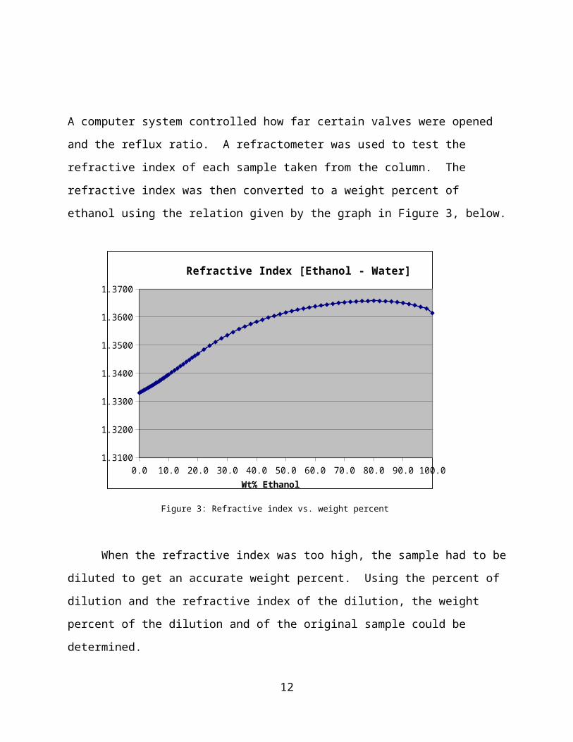
A computer system controlled how far certain valves were opened and the reflux ratio. A

refractometer was used to test the refractive index of each sample taken from the column. The

7

refractive index was then converted to a weight percent of ethanol using the relation given by the

graph in Figure 3, below.

0.0 10.0 20.0 30.0 40.0 50.0 60.0 70.0 80.0 90.0 100.01.3100

1.3200

1.3300

1.3400

1.3500

1.3600

1.3700

Refractive Index [Ethanol - Water]

Wt% Ethanol

When the refractive index was too high, the sample had to be diluted to get an accurate

weight percent. Using the percent of dilution and the refractive index of the dilution, the weight

percent of the dilution and of the original sample could be determined.

The chemical materials used in this experiment included ethanol, water, and ice. The

ethanol and water were combined in a feed tank that was pumped to the column to be separated.

The feed solution remained around 20 percent ethanol, by weight. The ice was used to cool

samples taken from the column before testing the refractive index to save time, since the

refractometer had to stabilize the temperature of the sample to the temperature of the room

before it could read the refractive index. Non-chemical materials include the distillation column,

the computer control system, the refractometer; a scale to help with the dilutions, sample tubes

and caps, graduated cylinders, a stopwatch, a Styrofoam cooler for the ice, disposable pipettes,

and boxes of Kim wipes to clean off the refractometer and the sample tubes.

8

Figure 3: Refractive index vs. weight percent ethanol

The column was started up by first turning on the computer system and checking for

errors and checking the liquid level in the feed tank. The air pressure, condenser water, cold-

water flow to the bottoms cooler, and steam were all turned on. The reboiler was heated by

setting the steam valve to 100% open. The feed rate was set at 9.4635*10-6 m3/s by adjusting the

feed control valve. After checking to make sure one of the feed tray valves was open to the

column, the feed pump was turned on.

The column was allowed to come to steady state after each variable tested was changed.

The column was left alone for 30 minutes. After 30 minutes, samples from the distillate and

bottoms were collected and the refractive indices were measured and the weight percent of

ethanol in each was calculated. When the weight percent of ethanol in the distillate and bottoms

varied by less than two percent between trials the column was said to be at steady state. To

ensure that steady state had been reached, 1*10-5 m3 of liquid was purged off of every tray and

the column was monitored for changes. If no changes were observed, samples were taken from

each tray, the distillate, bottoms, and feed tank. These samples were put on ice and the refractive

indices of each were measured in order to create a concentration profile for the column. Some

other parameters of the column were also recorded at this time. The next variable was then set,

and the column was allowed to come to steady state again, and the process was repeated. At all

stages, the column was monitored for signs of flooding. Once all variables were tested, the

column was shutdown.

The variables tested in this experiment were the feed tray number and the reflux ratio.

These two variables were tested because they offered the most measurable effects in the least

amount of time. Testing all of the variables that can be altered for a distillation column (feed

location, reflux ratio, bottoms product rate, feed rate, and steam rate) would have been too time

consuming to complete in one day. As it was, the reflux ratio trials were not completed on the

day of the experiment, and data had to be obtained from another group due to the ambient

temperature rising so high that the column was no longer functioning properly. The feed tray

location was tested at three locations: the third tray from the bottom, the sixth tray from the

bottom, and the ninth tray from the bottom. The reflux ratio was kept at 0.45 during these trials.

For the trials in which the reflux ration was changed, the feed tray was kept at the ninth tray from

the bottom, and the reflux ratios of 1 and 1.5 were tested. These five tests allowed for three

different feed tray locations to be tested and allowed for three different reflux ratios to be tested.

9

This ensured that any effect that these variables had on column operation would be clearly

discernible when the data were analyzed so that the best conclusions could be drawn.

The data collected from this experiment was used to analyze various aspects of the

column. These included the overall plate efficiency, minimum reflux ratio, Murphree plate

efficiency and overall MTC. In order to do these calculations a ChemCAD simulation was

employed in which conditions of the experiment were used as input parameters. From this

simulation, an equilibrium curve for ethanol in water was created. Composition data from the

experiment was then used to construct an operating line on the same plot. The McCabe-Thiele

method was used to find the theoretical number of stages this column would require which was

used, in turn, to find overall plate efficiency. Minimum reflux ratio was found using the pinch

point composition and equation (5). Murphree tray efficiency was found via a trial and error

method. The equilibrium curve had to be moved by a certain amount until the number of stages

stepped off from the operating line was equal to thirteen (twelve trays plus one reboiler).

Equation (7) was needed to find the overall MTC. The variables used in this equation were

calculated by experimentally observed data.

After calculating all of these values from the experimental data, it was compared to the

actual ChemCAD simulation data. This gave a good tool to evaluate the experimental data.

Comparisons were made between column concentration profiles, overhead distillate flow rate

and purity.

Some of the safety issues that had to be addressed during this experiment included the

temperature of the column, steam, and ambient air as well as the hazards of working with

chemicals such as ethanol, slipping, working near other large pieces of equipment, and working

with electronic equipment. Care was taken when taking samples from the column to avoid burns

from the hot samples and column. To avoid the adverse effects of using the hot steam, thermal

gloves were worn when turning the steam on and off. To deal with the high ambient air

temperatures, water bottles were a part of the personal protection equipment (PPE) list for each

experimenter and frequent water breaks outside of the laboratory were taken. The rest of the

required PPE included long sleeved shirts, long pants, closed-toed shoes with non-slip soles and

laces, safety splash goggles, hard hats, and nitrile gloves. The shirts, pants, shoes, goggles, and

nitrile gloves protected from skin exposure to ethanol. The non-slip shoes with tied laces

protected from slipping hazards when climbing the ladder to take samples from the column. The

10

hard hats provided protection from falling object hazards that can occur from the nature of

working in a laboratory setting with large pieces of equipment, such as the unit operations

laboratory. When working with electronic equipment, care was taken to not get the equipment

wet to avoid electrocution or short-circuit hazards.

11

Results and Discussion

After completing the distillation experiment, different values are calculated to determine

how well the column performed and its response to changing column conditions. In addition, the

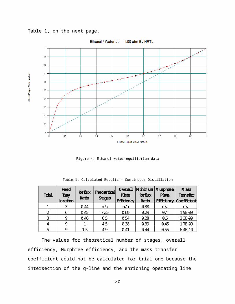
experimental data is compared to a computer-simulated model of the distillation column. Figure

4, below, is a graph of the equilibrium data prepared by ChemCAD. The minimum reflux ratio

is calculated by finding the “pinch point” or intersection of the q-line with the equilibrium curve

in Figure 4. In addition, the graph is used to evaluate the theoretical number of stages needed for

distillation by the McCabe-Thiele method. After acquiring the theoretical number of trays, the

overall plate efficiency is calculated and the Murphree plate efficiency is calculated by a trial and

error method. Plots using the McCabe-Thiele method and for finding Murphree plate efficiency

can be found in Appendix C. From the Murphree efficiency, the Mass Transfer Coefficient is

calculated using equation (7). These values are recorded in Table 1, on the next page.

Figure 4: Ethanol water equilibrium data

12

Table 1: Calculated Results – Continuous Distillation

Trial Feed Tray

Location

Reflux Ratio

Theoretical Stages

Overall Plate

Efficiency

Minimum Reflux Ratio

Murphree Plate

Efficiency

Mass Transfer

Coefficient1 3 0.44 n/a n/a 0.38 n/a n/a2 6 0.45 7.25 0.60 0.29 0.4 1.9E-093 9 0.46 6.5 0.54 0.28 0.5 2.3E-094 9 1 4.5 0.38 0.39 0.45 1.7E-095 9 1.5 4.9 0.41 0.44 0.55 6.4E-10

The values for theoretical number of stages, overall efficiency, Murphree efficiency, and

the mass transfer coefficient could not be calculated for trial one because the intersection of the

q-line and the enriching operating line occurred above the equilibrium line. This is shown in

Figure C1 in Appendix C. Since these parameters depend on there being space between the

operating lines and the equilibrium line or pinch point, they could not be determined. During

trial one, as soon as samples were taken from the column, the steam pressure began to rise, as

described in the error analysis section of this report. The crossing of the equilibrium line is most

likely due to this error and leads to the incomplete data in Table 1.

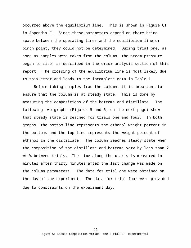
Before taking samples from the column, it is important to ensure that the column is at

steady state. This is done by measuring the compositions of the bottoms and distillate. The

following two graphs (Figures 5 and 6, on the next page) show that steady state is reached for

trials one and four. In both graphs, the bottom line represents the ethanol weight percent in the

bottoms and the top line represents the weight percent of ethanol in the distillate. The column

reaches steady state when the composition of the distillate and bottoms vary by less than 2 wt.%

between trials. The time along the x-axis is measured in minutes after thirty minutes after the

last change was made on the column parameters. The data for trial one were obtained on the day

of the experiment. The data for trial four were provided due to constraints on the experiment

day. As shown in the graphs, the column took a while longer to reach steady state and the

distillate composition fluctuated much more on the day that trial one was performed than

whenever trial four was performed, but both eventually reach steady state. For both trials, it can

be seen that the bottoms reach steady state much sooner than the distillate does.

13

0 5 10 15 20 25 30 35 400

0.1

0.2

0.3

0.4

0.5

0.6

0.7

0.8

0.9

1Liquid Composition vs. Time (Trial 1, Reaching Steady State)

Time (min)

Wei

ght F

ract

ion

Eth

anol

BottomsDistillate

Figure 5: Liquid Composition versus Time (Trial 1) –experimental

0 1 2 3 4 5 6 7 8 9 100

0.1

0.2

0.3

0.4

0.5

0.6

0.7

0.8

0.9Liquid Composition vs. Time (Trial 4, Reaching Steady State)

Time (min)

Wei

ght F

ract

ion

Eth

anol

BottomsDistillate

Figure 6: Liquid Composition versus Time (Trial 4) –experimental

14

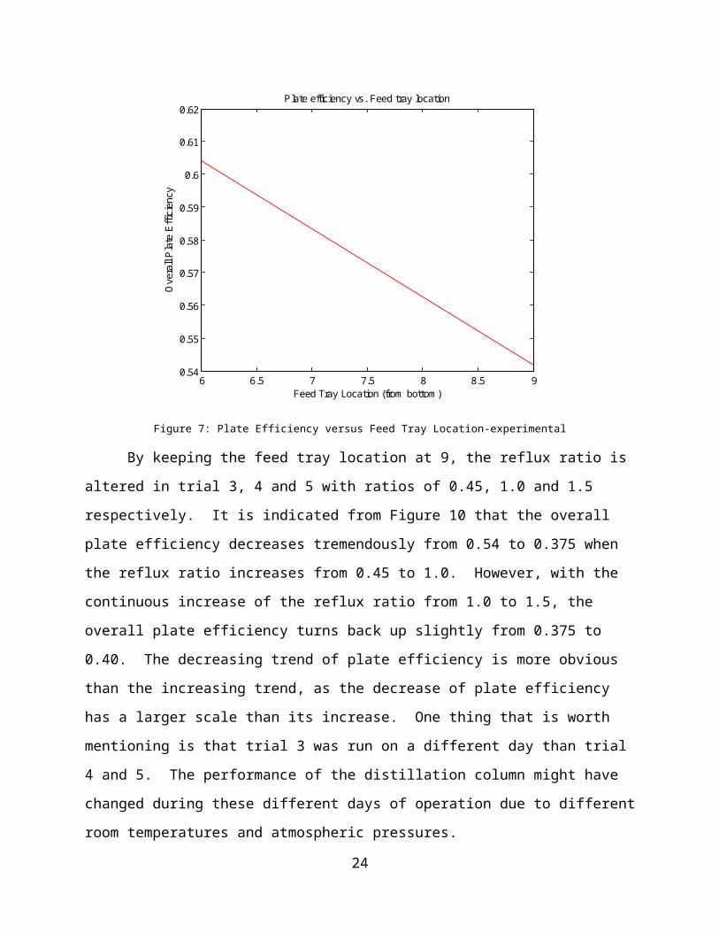
The plate efficiency versus feed tray is plotted in Figure 7. In this figure, feed tray

location 6 and 9 from the bottom with the same reflux ratio of 0.45 are used from Trials 2 and 3,

respectively, to examine the relationship with plate efficiency. Trial 1 with feed location 3,

however, is not used, as the intersection point of q line and enriching line in the McCabe-Thiele

diagram is above the vapor liquid equilibrium curve as described earlier and in the error analysis.

Because of this, the theoretical stages are not able to be determined using the equilibrium data.

The experimental data calculated by the McCabe-Thiele method in Figure 7 illustrates that with

the higher feed location the overall plate efficiency tends to decrease. However, there are only

two points presented in this figure thus a valid trend cannot be determined.

6 6.5 7 7.5 8 8.5 90.54

0.55

0.56

0.57

0.58

0.59

0.6

0.61

0.62Plate efficiency vs. Feed tray location

Feed Tray Location (from bottom)

Ove

rall

Pla

te E

ffici

ency

Figure 7: Plate Efficiency versus Feed Tray Location-experimental

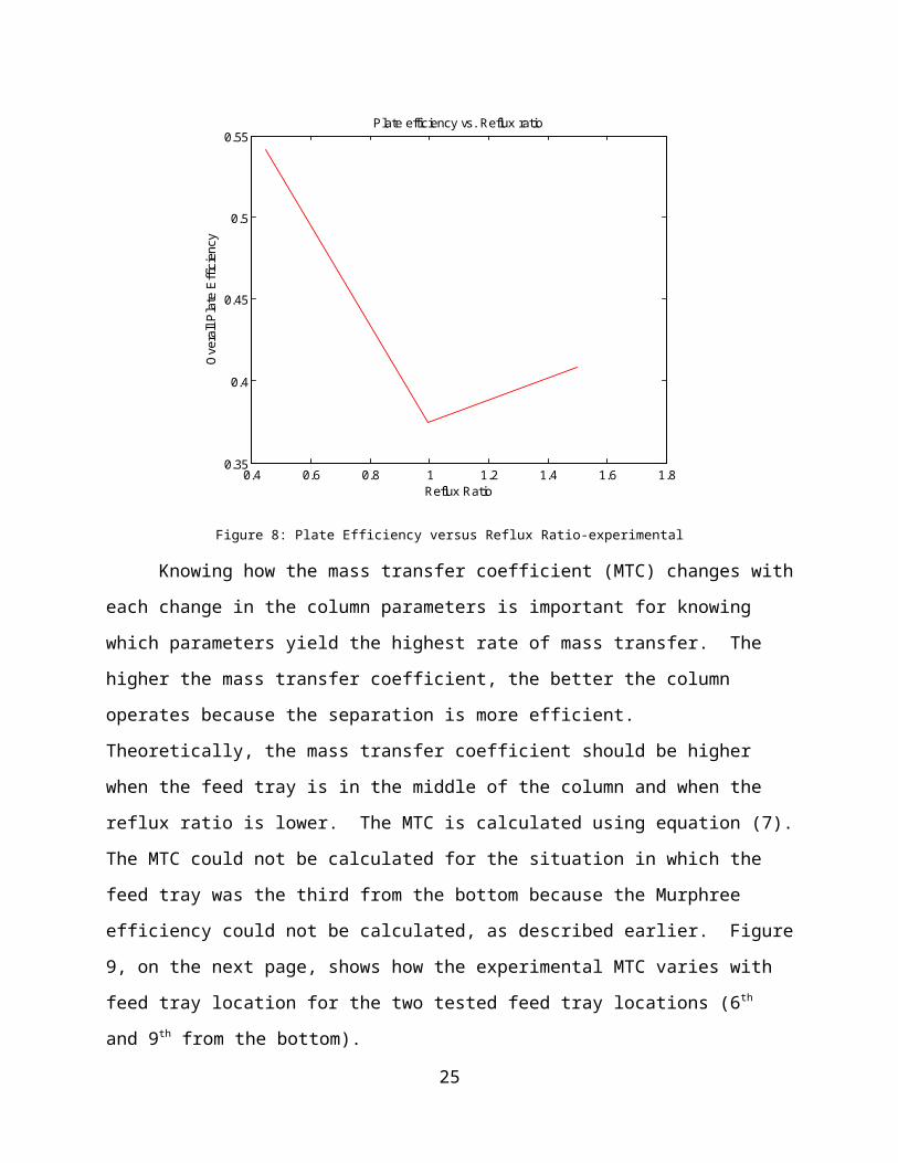
By keeping the feed tray location at 9, the reflux ratio is altered in trial 3, 4 and 5 with

ratios of 0.45, 1.0 and 1.5 respectively. It is indicated from Figure 10 that the overall plate

efficiency decreases tremendously from 0.54 to 0.375 when the reflux ratio increases from 0.45

to 1.0. However, with the continuous increase of the reflux ratio from 1.0 to 1.5, the overall

plate efficiency turns back up slightly from 0.375 to 0.40. The decreasing trend of plate

efficiency is more obvious than the increasing trend, as the decrease of plate efficiency has a

larger scale than its increase. One thing that is worth mentioning is that trial 3 was run on a

15

different day than trial 4 and 5. The performance of the distillation column might have changed

during these different days of operation due to different room temperatures and atmospheric

pressures.

0.4 0.6 0.8 1 1.2 1.4 1.6 1.80.35

0.4

0.45

0.5

0.55Plate efficiency vs. Reflux ratio

Reflux Ratio

Ove

rall

Pla

te E

ffici

ency

Figure 8: Plate Efficiency versus Reflux Ratio-experimental

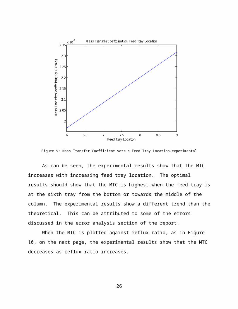
Knowing how the mass transfer coefficient (MTC) changes with each change in the

column parameters is important for knowing which parameters yield the highest rate of mass

transfer. The higher the mass transfer coefficient, the better the column operates because the

separation is more efficient. Theoretically, the mass transfer coefficient should be higher when

the feed tray is in the middle of the column and when the reflux ratio is lower. The MTC is

calculated using equation (7). The MTC could not be calculated for the situation in which the

feed tray was the third from the bottom because the Murphree efficiency could not be calculated,

as described earlier. Figure 9, on the next page, shows how the experimental MTC varies with

feed tray location for the two tested feed tray locations (6th and 9th from the bottom).

16

6 6.5 7 7.5 8 8.5 9

2

2.05

2.1

2.15

2.2

2.25

2.3

2.35x 10

-9

Feed Tray Location

Mas

s Tr

ansf

er C

oeffi

cien

t, K

y (1

/Pa-

s)

Mass Transfer Coefficient vs. Feed Tray Location

Figure 9: Mass Transfer Coefficient versus Feed Tray Location-experimental

As can be seen, the experimental results show that the MTC increases with increasing

feed tray location. The optimal results should show that the MTC is highest when the feed tray

is at the sixth tray from the bottom or towards the middle of the column. The experimental

results show a different trend than the theoretical. This can be attributed to some of the errors

discussed in the error analysis section of the report.

When the MTC is plotted against reflux ratio, as in Figure 10, on the next page, the

experimental results show that the MTC decreases as reflux ratio increases.

17

0.4 0.6 0.8 1 1.2 1.4 1.6 1.80.6

0.8

1

1.2

1.4

1.6

1.8

2

2.2

2.4x 10

-9

Reflux Ratio

Mas

s Tr

ansf

er C

oeffi

cien

t, K

y (1

/Pa-

s)

Mass Transfer Coefficient vs. Reflux Ratio

Figure 10: Mass Transfer Coefficient versus Reflux Ratio-experimental

These results match the theoretical ones. This indicates that the best reflux ratio, in terms

of MTC is a lower value. Overall, based on the experimental results, the best feed tray location

is the highest one (ninth from the bottom) and the best reflux ratio is the lowest one (in this case,

0.45).

To test the validity of the experimental results, an ideal column can be run using the

ChemCAD computer program. A useful comparison between the experimental results and the

ChemCAD model is the liquid composition along the column at each tray. This can be easily

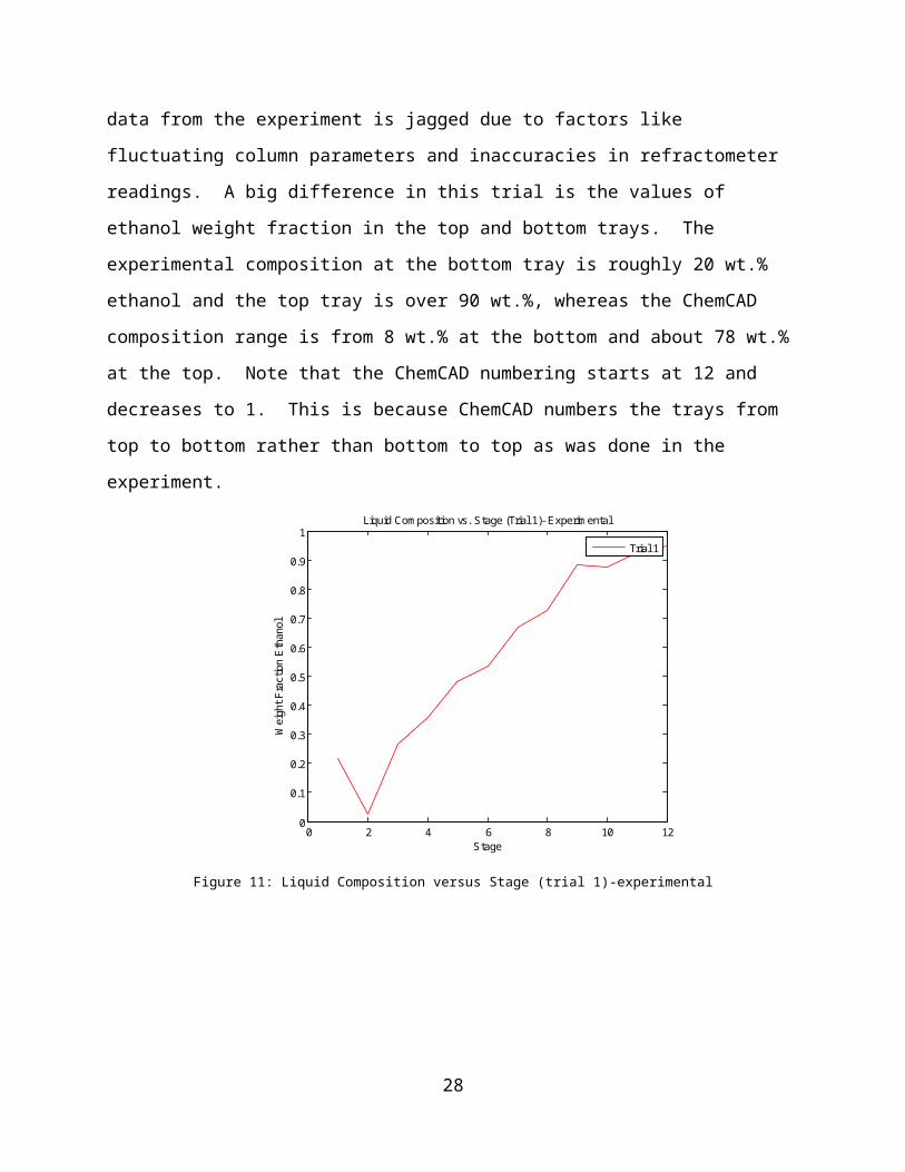
done by observing the trends in Figures 11 and 12. Figure 11, the experimental column

concentration profile, shows a general increase in weight fraction of ethanol as it gets higher in

the column. The same trend is seen Figure 12, the ChemCAD concentration profile, though it is

a much smoother curve. The data from the experiment is jagged due to factors like fluctuating

column parameters and inaccuracies in refractometer readings. A big difference in this trial is

the values of ethanol weight fraction in the top and bottom trays. The experimental composition

at the bottom tray is roughly 20 wt.% ethanol and the top tray is over 90 wt.%, whereas the

ChemCAD composition range is from 8 wt.% at the bottom and about 78 wt.% at the top. Note

18

that the ChemCAD numbering starts at 12 and decreases to 1. This is because ChemCAD

numbers the trays from top to bottom rather than bottom to top as was done in the experiment.

0 2 4 6 8 10 120

0.1

0.2

0.3

0.4

0.5

0.6

0.7

0.8

0.9

1Liquid Composition vs. Stage (Trial 1)- Experimental

Stage

Wei

ght F

ract

ion

Eth

anol

Trial 1

Figure 11: Liquid Composition versus Stage (trial 1)-experimental

Figure 12: Liquid Composition versus Stage (trial 1)-ChemCAD

To give a better comparison, trial 2 is also examined in Figures 13 and 14 on the next

page. The experimental results from trial 2 seem to fit the ChemCAD results a little better than

in trial 1. Again, a discrepancy exists between some of the values, most evident in the bottom

19

tray where the experimental gives a value of 21 wt.% ethanol and the ChemCAD shows just 7.5

wt.%. However, in this case the weight fraction of ethanol in the top tray for both the

experimental and ChemCAD is just under 0.8. Corresponding column concentration profiles for

trials 3 through 5 can be found in Appendix E.

0 2 4 6 8 10 120.2

0.3

0.4

0.5

0.6

0.7

0.8

0.9Liquid Composition vs. Stage (Trial 2)- Experimental

Stage

Wei

ght F

ract

ion

Eth

anol

Trial 2

Figure 13: Liquid Composition versus Stage (trial 2)-experimental

Figure 14: Liquid Composition versus Stage (trial 2)-ChemCAD

20

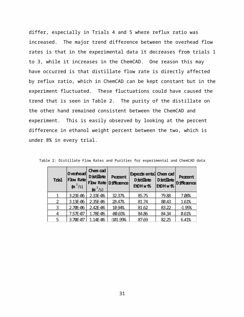
Distillate flow rate and purity can also be compared between the experiment and

ChemCAD simulation. As shown in Table 2, below, the experimental and ChemCAD data for

overhead flow rate differ, especially in Trials 4 and 5 where reflux ratio was increased. The

major trend difference between the overhead flow rates is that in the experimental data it

decreases from trials 1 to 3, while it increases in the ChemCAD. One reason this may have

occurred is that distillate flow rate is directly affected by reflux ratio, which in ChemCAD can be

kept constant but in the experiment fluctuated. These fluctuations could have caused the trend

that is seen in Table 2. The purity of the distillate on the other hand remained consistent between

the ChemCAD and experiment. This is easily observed by looking at the percent difference in

ethanol weight percent between the two, which is under 8% in every trial.

Table 2: Distillate Flow Rates and Purities for experimental and ChemCAD data

Trial Overhead Flow Rate

(m3/s)

Chemcad Distillate Flow Rate

(m3/s)

Percent Difference

Experimental Distillate EtOH wt%

ChemcadDistillate EtOH wt%

Percent Difference

1 3.23E-06 2.33E-06 32.37% 85.75 79.88 7.08%2 3.13E-06 2.35E-06 28.47% 81.74 80.43 1.61%3 2.70E-06 2.42E-06 10.94% 81.62 83.22 -1.95%4 7.57E-07 1.78E-06 -80.65% 84.86 84.34 0.61%5 3.70E-07 1.14E-06 -101.99% 87.69 82.25 6.41%

21

Error AnalysisDistillation is a complicated process that requires comprehensive control over the process

variables as they affect column performance. During the operation of the column, there were

several internal and external variables adversely affecting the recorded data, especially the vapor

composition. In addition, steady-state operation was not easily achieved and usually took a long

time to reach due to fluctuations in process variables.

One source of possible error was the ambient temperature. This parameter was an

external variable that could not be controlled and adversely affected the operation of the column.

The pressure drop from the bottom to the top of the column would fluctuate and was dangerously

close to its upper limit. The high external temperature led to anomalies in the recorded data and

limited the experiment to only 3 of the required 5 trials, meaning that data for the last two trials

had to be obtained from another group. In addition, the temperature was causing the column to

overheat and did not allow the column to reach steady-state quickly. This is shown by the

multiple attempts to find the steady-state distillate weight percent and the seven to eight readings

needed before steady state was reached. Because of the length of time needed to reach steady

state and the continued fluctuations in readings after steady state was thought to have been

reached, the data recorded was unreliable.

The valves that control the flow through the column also could lead to error introduced

into the experiment. The computer system controls the feed flow rate by controlling the amount

that the feed pipe, bottoms product flow, and reflux valves are opened. In particular, the feed

flow rate would be set at around 0.0095 m3/s, but it would decrease below the set point after a

period of time, even if unprovoked due to the faulty valves. This led to prolonged waits for

steady-state to be reached as well as the possibility of the concentrations recorded at the wrong

feed flow rate. This could increase the deviation from the ideal column modeled in ChemCAD.

In effect, this would lower the plate efficiencies.

A third source of error was the refractometer. Many times the refractometer would give

two different refractive indices (RI) for the same sample if two measurements were taken of the

sample. This meant the real RI of a particular sample could remain unknown, and therefore the

real weight percent of the sample could remain unknown. The data would then be skewed

because of this error. It was often unclear as to whether the data from the refractometer was

correct or not. If two measurements from the same sample were taken and yielded different

22

readings, it was difficult to know which one was correct and which one was the wrong reading.

Since the sample taken from the column and the time constraints only allowed for one or two

tests on the refractometer, the one that more closely matched the expected trends was chosen,

which could mean that samples were taken too soon or conclusions were incorrectly drawn.

A fourth source of error was the volatility of ethanol. For the samples that were higher

than fifty weight percent ethanol, the sample had to be diluted with water in order to get an

accurate weight percent calculation from the measured refractive index. In the time it took to

transfer some sample to a clean tube, weigh it, record the weight, zero the scale, add water,

weigh and record the weight of the water, and then take the refractive index, some of the ethanol

in the sample would have evaporated. This caused an inaccurate sample weight to be recorded

as well as an inaccurate refractive index to weight percent calculation. The refractometer also

took a long time to alter the temperature of the sample to 293 K and to measure the refractive

indices of the samples, allowing time for some of the ethanol to evaporate and giving results that

were lower in weight percent than they should have been.

Another source of error occurred when taking steady state readings for trial 1. It was

noted that the steam pressure began to increase significantly as soon as samples were taken from

the column, although the purging of the column had not affected the steam pressure. Samples

were taken starting from the top of the column and working down. Since the distillate faucet was

at the bottom of the column, it was taken as one of the last readings. The rise in steam pressure

and the time between taking the samples from the top of the column and the distillate caused a

significant difference in the readings from the two. It was found that the distillate had a lower

weight percent of ethanol that the top three trays did, which is a result that should never occur in

a distillation column. The results of this trial were such that the q line and enriching operating

line crossed above the equilibrium line, meaning that none of the analysis methods could be used

to analyze this trial. This could stem from the fact that the pressure rose so quickly while

samples were taken.

To demonstrate the effect of all of these sources of error, Table 2 shows the differences

between the data obtained experimentally and the ideal data given by the ChemCAD analysis.

23

Conclusions

The objective of this experiment is to explore the operation of a continuous distillation

column and study the sensitivity to changing different process variables. However, due to time

constraints and exceedingly high ambient temperature the complete experiment could not be

finished as well as a complete study on the sensitivity of the column. In addition, for the first

trial, the plate efficiencies and mass transfer coefficient were not calculated because the

enriching operating line intersected the equilibrium curve above the pinch point. Thus, the

McCabe-Thiele method would indicate that the theoretical number of trays was infinite. This

means that when analyzing the data, there is one less data point in an already small data set.

However, from the data collected there are still trends and conclusions that can be made.

The feed tray location is one of the controlled variables in this study and from the data

collected; it is noticeable that this parameter affects the performance of the column. The degree

of this influence is difficult to state from this experiment because of the limited number of data

points. However, due to the trend of higher overall tray efficiency towards the middle of the

column it can be deduced that the location of the feed tray in the middle of the column is most

favorable for column performance. In Table 1 and Figure 7, it shows that with the feed tray at

tray 6 from the bottom, the overall plate efficiency is 0.60 and when the feed tray location is at 9,

the plate efficiency is 0.54. It is difficult to ensure from this data that this is completely accurate,

but from experience with distillation columns, this is known to be accurate.

The other variable controlled was the reflux ratio. This data is more complete and leads

to a more thorough conclusion. With increasing reflux ratio, the overall plate efficiency and the

mass transfer coefficient decreased. That is to say, that a lower reflux ratio is better for column

performance from the data collected.

Finally, it can be concluded that the methods used to calculate the plate efficiencies

especially the Murphree efficiency are inexact and not as rigorous as needed to be to make clear

conclusions. In addition, the ambient conditions of the column need to be maintained to ensure

proper function of the column and reliable data is collected. This is most evident by comparing

the experimental data to the theoretical ChemCAD simulation. The inconsistencies in

experimental data are highlighted by the trends offered by the ChemCAD. The differences are

displayed in Table 2.

24

RecommendationsTo improve this experimental set-up and analysis, the following recommendations are

made:

First, the surroundings of the column can be changed. Moving the column to an

enclosed, insulated room, with air conditioning and heating capabilities to stabilize the ambient

temperature would greatly reduce the amount of error caused by the high ambient temperatures

of late June. One of the greatest sources of error for this experiment was that the ambient

temperature, and therefore the temperature of the column, rose quite significantly during the

course of the experiment, causing the column to not reach steady-state reliably and causing the

data to be skewed. The data would be much more reliable if the ambient temperature could have

been controlled and maintained at a constant value.

Another recommendation that can be made to improve the data obtained from the column

is to install better valves throughout the column. One of the bigger factors stopping the column

from reaching steady state quickly was the fact that the feed valve did not adequately control the

flow rate of the feed stream. The valve had to be continually opened and closed by percentages

to maintain the desired feed flow rate. The flow rate kept dropping below the desired flow rate

while the column was reaching steady state. Every time that the feed flow rate was altered, it

took longer for the column to reach steady state. A valve that controlled the flow rate through it

more reliably would be a huge asset to the operation of the column.

A third recommendation would be to find another way of determining the concentration

of ethanol in water. The refractometer was unreliable in its readings. A better-calibrated

refractometer could solve this problem. The concentration of ethanol in water can also be

calculated by taking a mass and volume reading for each sample and calculating concentration

from the known densities or specific gravities of water and ethanol. This method would involve

having tubes that had volume scales on the sides (similar to beakers) that would be weighed with

the cap before and after sample was added. This way, the cap could remain on the tube at all

times when the sample was in the tube, and not allow for any of the sample to evaporate.

Dilutions would not need to be done, and the error-prone refractometer would not need to be

used.

25

Design Extension

The objective of the design extension problem was to specify the optimal design of a

distillation column which separates 86 wt.% of methanol from a methanol and n-propanol

mixture. The product had to be 86 wt.% of methanol. The feed flow rate was 6250 kg/hr,

consisted of 17 wt.% methanol and 83 wt.% n-propanol, and enters at a temperature of 296 K

and a pressure of 101,325 Pa. The optimal number of stages and feed location that provides the

desired purity with highest energy efficiency needed to be calculated. The possible number of

trays varied from 10 to 100.

In order to simulate the energy consumption for different numbers of stages and feed tray

locations, a ChemCAD computer simulation program was used to collect data for the reboiler

and condenser duties for each situation and then the data were plotted using Excel. As can be

seen from Figures 15 and 16, below and on the next page, the reboiler and condenser duty first

decreased dramatically with increasing number of stages and then they fluctuated slightly.

10 20 30 40 50 60 70 80 90 1002905

2955

3005

3055

3105

3155Number of Stages vs. Reboiler

Duty

Number of Stages

Rebo

iler D

uty(

MJ/

hr)

26

Figure 15: Number of Stages vs. Reboiler Duty

10 20 30 40 50 60 70 80 90 100

-2100-2050-2000-1950-1900-1850-1800-1750-1700-1650

Number of Stages vs. Condenser Duty

Number of Stages

Cond

ense

r Dut

y(M

J/hr

)

As the lowest reboiler and condenser duties were found between 30 to 40 stages, the scale

of the plot was narrowed to this region. Figures E7 and E8 in Appendix E indicate that the

lowest reboiler and condenser duties are achieved when the number of stages were 31 and 36

respectively. The number of stages versus total energy consumption was plotted in Figure 17,

below. The total energy consumption is the summation of the absolute value of reboiler duty and

condenser duty. As it is indicated, with 36 stages, the total energy consumption was the lowest.

As a result, the optimal number of stages was 36.

30 31 32 33 34 35 36 37 38 39 404717

4718

4719

4720

4721

4722

4723

Number of Stages vs. Total Energy Consumption

Number of Stages

Tota

l Ene

rgy

Cons

umpti

on (M

J/hr

)

27

Figure 16: Number of Stages vs. condenser Duty

Figure 17: Number of Stages vs. Reboiler Duty

Once the number of stages was determined, the range of feed locations could be

narrowed to between trays 1 and 36. The feed location versus reboiler duty and condenser duty

were plotted in Figures E9 and E10 in the Appendix E. From these two figures, it can be seen

that the lowest reboiler and condenser duties were found in feed tray locations of tray 17 and tray

18, respectively. In order to choose only one feed location, the relationship between feed tray

location and total energy consumed was also examined. As can be seen from Figure 16, below,

the most energy efficient feed tray location was the 17th tray from the top.

10 11 12 13 14 15 16 17 18 19 20 21 22 23 24 25 264716

4717

4718

4719

4720

4721

4722

4723

4724

4725Feed Location vs. Total Energy

Consumption

Feed Location

Tota

l Ene

rgy

Cons

umpti

on (M

J/hr

)

Thus, the optimal number of stages was 36 and the optimal feed tray location was tray 17

from the top. The reboiler duty and condenser duty were 808258 J/s and -502533 J/s. The reflux

ratio for these parameters was 0.856596. With these parameters, the total energy consumption

was the lowest.

The reason that feed tray location has such a great impact on energy consumption is that

if the feed tray location is high, there are more stripping trays are available, which cause a lower

reboiler duty. However, higher feed locations also require high liquid flow, which increases the

reboiler duty on the opposite side. If the feed location is too low, more energy is needed to heat

and vaporize the liquid to the top of the column, and more liquid is stuck in the lower level of the

column. (Khoury, 2005). Due to the combination of these two effects, the energy consumption

is changed by changing feed location. As a result, finding the optimal number of trays and feed

tray location is essential to reduce the energy consumption.

28

Figure 18: Feed location vs. Total Energy Consumption

NotationTable 3: Notation

Notation Annotation Units

V Vapor Flow Rate m3/s

L Liquid Flow Rate m3/s

xn Mole Fraction in Liquid

yn Mole Fraction in Vapor

xD Mole Fraction in Distillate

xW Mole Fraction in Bottoms

xF Mole Fraction in Feed

R Reflux Ratio

q Feed Condition

HV Feed Enthalpy at Dew Point kJ/mol

H L Feed Enthalpy at Boiling Point kJ/mol

H F Feed Enthalpy at Entrance Conditions

kJ/mol

Rm Minimum Reflux Ratio

EM Murphree Tray Efficiency

EOG Gas-phase Tray Efficiency

29

Notation Annotation Units

a Specific Area m2/m3

G Superficial Molar Velocity m/s

hL Pressure Drop per Tray Pa

K y Mass Transfer Coefficient (MTC) Pa-1-s-1

EtOH Ethanol

wt.% Weight Percentage or component percentage by weight (%)

RI Refractive index

30

Literature Cited

APEC Water. "Different Water Filtration Methods Explained." Different Water Filtration

Methods. N.p., n.d. Web. 01 July 2012. <http://www.freedrinkingwater.com/water-

education/quality-water-filtration-method.htm>.

ITT Tech."Distillation and Alcohol Production Application"N.p., 2012.Web. 27 June 2012.

http://www.docstoc.com/docs/116873123/Distillation-and-Alcohol-Production-

Application

Geankoplis, Christie J. 2010, Transport Processes and Separation Process, page 707-726

GEC Process Engineering Inc. "Distillation Applications.” Distillation Technology and. N.p.,

n.d. Web. 01 July 2012. <http://www.niroinc.com/evaporators_crystallizers/distil-

lation.asp>.

Khoury, Fouad M. Multistage Separation Processes. Boca Raton: CRC, 2005. Print. Pg.222

Mangino, Michael E. “Protein Denaturation.” Food Science 822. 2007. Web. 2 July 2012.

<http://class.fst.ohio-state.edu/FST822/lectures/Denat.htm>.

Riggs, Jim. "Distillation: Introduction to Control - Practical Process Control by Control Guru."

N.p., 2008. Web. 27 June 2012. <http://www.controlguru.com/wp/p60.html>.

Tham, M.T. "Distillation: an Introduction." Distillation Column Design N.p.,1997. Web. 27 June

2012. <http://lorien.ncl.ac.uk/ming/distil/distildes.htm>

Treybal, Robert E. Mass Transfer Operations. New York, McGraw-Hill Book Co., 1980. SEL

Reserve: TP156.M3 T7 1980.

31