Calibration Procedure Developed for FMC-TFM Based Imaging System

Michael Wright, Jonathan Lesage, Mohammad Marvasti, Steven Peters, Mike Matheson

Acuren Research and Application Development Group, Cambridge, Ontario, Canada

Abstract

In recent years, there has been an increasing interest in the Full Matrix Capture (FMC) data acquisition method within the Non-Destructive Testing (NDT) industry. The FMC approach involves transmitting with each element in a phased array probe in sequence, while capturing the response with all elements. The captured data can be post-processed to produce detailed, high resolution images of the test piece, most commonly by applying the Total Focusing Method (TFM), which effectively focuses ultrasonic energy at every pixel. The resulting images are typically much easier to interpret than traditional phased array sweeps and can lead to a higher probability of detection of indications while decreasing data analysis time. It seems likely that FMC-TFM based systems will eventually come to dominate the NDT industry, provided that a proper calibration procedure can be developed to meet existing inspection codes. To this end, a novel, measurement based, calibration procedure developed by Acuren’s Research and Application development group is presented, implemented and assessed based on phased array ultrasonic code requirements. The results of the present study indicate that the proposed calibration procedure can effectively calibrate amplitudes close to the center of the aperture, though cannot meet existing code requirements over the entire aperture for shallow targets. The source of the incomplete amplitude compensation is identified and further research to mitigate these effects are proposed.

1. FMC – TFM Introduction

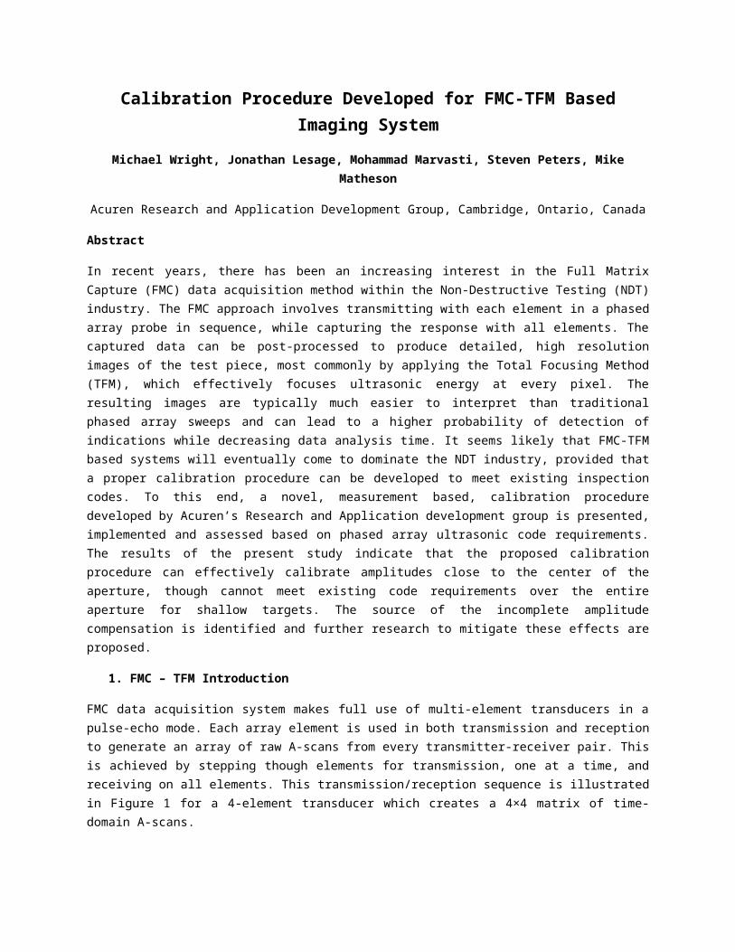
FMC data acquisition system makes full use of multi-element transducers in a pulse-echo mode. Each array element is used in both transmission and reception to generate an array of raw A-scans from every transmitter-receiver pair. This is achieved by stepping though elements for transmission, one at a time, and receiving on all elements. This transmission/reception sequence is illustrated in Figure 1 for a 4-element transducer which creates a 4×4 matrix of time-domain A-scans.

Figure 1 FMC Acquisition Using a 4-Elemenet Probe.

The acquired A-scans are then synthetically focused at every point in the test piece to produce a high quality image using the Total Focusing Method. The TFM algorithm builds an image by first calculating time it takes for an ultrasonic wave to travel between each transmit/receive element pair to each pixel point in a domain and then assigning the amplitude corresponding to the calculated travel time from the A-scan to the corresponding pixel

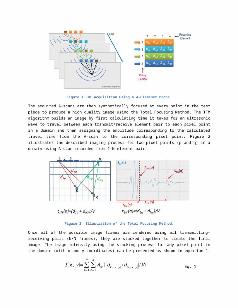
point. Figure 2 illustrates the described imaging process for two pixel points (p and q) in a domain using A-scan recorded from 1-N element pair.

Figure 2 Illustration of the Total Focusing Method.

Once all of the possible image frames are rendered using all transmitting-receiving pairs (N×N frames), they are stacked together to create the final image. The image intensity using the stacking process for any pixel point in the domain (with x and y coordinates) can be presented as shown in equation 1:

I ( x , y )=∑m=1

N

∑n=1

N

Amn((dm, ( x , y )+dn , ( x , y ) )/V ) Eq. 1

Using the above stacking routine, high amplitude values get stacked at locations where reflectors are present while very low amplitudes get stacked at locations where no reflectors exist. This procedure results in a very sharp, high quality image, owing to the fact that all of the collected A-scans are effectively focused at every pixel point in the domain. Figure 3 shows the difference between a TFM images built using a single Frame (1 Transmitting Element, N receiving Elements) to a TFM image built by stacking N frames (N Transmitting Elements, N receiving Elements).

Figure 3 shows that, although a sharp, high quality image has been obtained by application of the TFM, image intensities are not uniform across the imaging range. The four indications originate from holes which were the same size and differing only in terms of their relative position with respect to the center of array aperture. This can be largely explained by the effects of element directivity and beam spread. Ultrasonic energy decreases away from the center of a transmitting element – this effect is referred to as element directivity. As a consequence of directivity, reflectors are insonified with decreasing levels of energy, the farther they are from an element’s central axis (as measured by angle with respect to the element’s centerline). In addition to the effects of directivity, ultrasonic energy decreases with distance from the element’s surface. The loss of energy with increased travel path is due to the combined effects beam spread – caused by the wave front spreading out to cover larger volumes as the wave progresses, and material attenuation due to scattering, and dissipative sources. In steels and most other commonly inspected materials, the loss of energy with travel path is dominated by the beam spread effect. Both directivity and Beam Spread lead to the distribution of ultrasonic energy, generated by an element to be non-uniform over the inspection region.

Figure 3 Effect of Stacking TFM Frames.

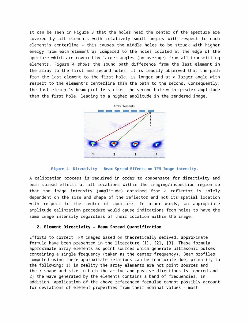
It can be seen in Figure 3 that the holes near the center of the aperture are covered by all elements with relatively small angles with respect to each element’s centerline – this causes the middle holes to be struck with higher energy from each element as compared to the holes located at the edge of the aperture which are covered by larger angles (on average) from all transmitting elements. Figure 4 shows the sound path difference from the last element in the array to the first and second holes. It is readily observed that the path from the last element to the first hole, is longer and at a larger angle with respect to the element’s centerline than the path to the second. Consequently, the last element’s beam profile strikes the second hole with greater amplitude than the first hole, leading to a higher amplitude in the rendered image.

Figure 4 Directivity - Beam Spread Effects on TFM Image Intensity.

A calibration process is required in order to compensate for directivity and beam spread effects at all locations within the imaging/inspection region so that the image intensity (amplitude) obtained from a reflector is solely dependent on the size and shape of the reflector and not its spatial location with respect to the center of aperture. In other words, an appropriate amplitude calibration procedure would cause indications from holes to have the same image intensity regardless of their location within the image.

2. Element Directivity – Beam Spread Quantification

Efforts to correct TFM images based on theoretically derived, approximate formula have been presented in the literature [1], [2], [3]. These formula approximate array elements as point sources which generate ultrasonic pulses containing a single frequency (taken as the center frequency). Beam profiles computed using these approximate relations can be inaccurate due, primarily to the following: 1) in reality the array elements are not point sources and their shape and size in both the active and passive directions is ignored and 2) the wave generated by the elements contains a band of frequencies. In addition, application of the above referenced formulae cannot possibly account for

deviations of element properties from their nominal values - most significant of which are: the element width, element spectrum and uniform displacement over the element’s surface. For the above stated reasons, it is preferable to directly measure the beam profile, where possible.

A new approach is introduced in the present study to directly estimate the average beam profile (taken to be representative of all elements in the array once element sensitivity is calibrated for) using measured A-Scans obtained from the specular reflection between all element pairs. The theoretical basis of the new approach is explained in this section, testing the approach in terms of a calibration process and then correction of the TFM images to use the calculated directivity and beam spread effects are presented in the next sections.

Consider a multi element array in contact with a block with a known thickness Th, as shown in Figure 5. The beam path from the center of the first element to the center of the ‘n-th’ element of the aperture after being reflected from the back wall is shown using two blue arrows. Beam angles and the total sound path length between the two elements can be obtained using Equations 2 and 3 respectively where p is the elements pitch.

Figure 5 Array Elements Beam Paths to the Backwall.

θ1−n=tan−1 (n−1 ) p /2Th Eq. 2 d1−n=

2×Thcosθ1−n Eq. 3

A-Scan signal recorded by pulsing on element 1 and receiving on element n (S1-n) contains a peak amplitude at time t = d1-n/V, equivalent to the time it takes for the sound to travel along d1-n path.

The peak amplitude can be modeled mathematically using Equation 4 where A1 and An represent elements sensitivity, R, represent angle dependent reflection coefficient and C represents the beam profile as a result of sound wave propagation off the center of the element (directivity) and travel path (beam spread).

A1−n=A1×C (θ1−n , d1−n ) × R (θ1−n )× C (θ1−n , d1−n )× An Eq. 4

The above equation can be rearranged to obtain the beam profile for ϴ1-n angle and d1-n distance combinations:

C (θ1−n , d1−n )=√ A1−n

A1 An R (θ1−n ) Eq. 5

The beam profile can be calculated using Equation 5 by knowing the right side of the equation: 1) A1-n can be measured as described above; 2) Reflection coefficient R values as a function of incident angle on a steel-air boundary are presented in literatures [4] and 3) A1 and An values can be measured with respect to a reference amplitude by comparing peak amplitudes corresponding to the first backwall on the pulse echo signals obtained from each element. Repeating the above described approach using sound paths between any 2 elements of the aperture can lead to calculating the beam profile for more angle – sound path combinations. The combination can be increased further when the array is in contact with blocks with different thicknesses. The beam profile calculated for these discrete number of angle-sound path combinations can be used to obtain beam profile for angle-sound path

combinations of all pixel points in a TFM image using interpolation. The interpolated beam profile at each pixel point can then be used to create a correction factor to compensate for directivity and beam spread effects in a TFM image.

3. Proposed Calibration Procedure

The calibration process includes velocity calibration, probe delay calibration, sensitivity calibration and finally calibration for directivity and beam spread effects. A calibration block has been designed and manufactured to perform all calibration steps. The calibration block was designed to contain 6 steps with 0, 28, 46, 64, 82 and 100 mm heights as shown in Figure 6.

Figure 6 Step Calibration Block and Calibration Process.

The proposed calibration procedure can be summarized as follows:

1) Velocity calibration is performed by comparing travel time between two consecutive backwall echoes on A-scans captured when an element is used in transmit mode and the same element is used in receiving mode. The measured travel time is used with the block thickness to calculate velocity.

2) Probe delay calibration is required to compensate for time delay in pulsing between different elements. A-scans obtained from each element in a pulse echo mode is used for calibration. Time corresponding to the peak amplitude from first backwall reflection is recorded from each element’s pulse-echo A-scan. Recorded times were compared to obtain elements pulsing time delays.

3) Sensitivity calibration is required to compensate for variation in energy transmitted by each element. The peak amplitude corresponding to the first backwall reflection is recorded from each element’s pulse-echo A-scan. Peak amplitude values are normalized with respect to the maximum amplitude recorded. The normalization factor used for each element can be used to compensate for differences in energy generated by each element.

4) Calibration for directivity and beam spread is performed by calculating the beam profile generated by each array element. The probe is placed on each step of the calibration block individually and FMC data is captured. The recorded A-Scans from each step are used to calculate beam profile as explained in section 3 (using Equation 5). All angle-sound path combinations provided by the aperture length and varying block thickness that are under the aperture in each step are evaluated. Angle and sound path combinations can be converted to x and y coordinates and the measured beam profile on these coordinates is used to interpolate the beam profile on a uniform x-y grid.

A 5L64-A2 Olympus array probe (64 elements, 5 MHz center frequency, 0.6 mm pitch) was used to scan the step block shown in Figure 6. A Micropulse, 128 Element Phased Array channel PeakNDT instrument was used to collect FMC data at a sampling frequency of 25 MHz. The interpolated beam profile, C(x,y) obtained using this calibration procedure has been plotted in Figure 7. The beam profile has been interpolated in the regions that data points were obtained. The beam profile was found to be roughly symmetric about the element’s centerline (x=0) and drops off away from the centerline and as y increases which is consistent with directivity and beam spread effects.

Figure 7 Beam Profile Interpolated on a uniform x-y grid.4. Beam Profile Based Correction Factor

The beam profile obtained through the calibration process explained in the previous sections has been used to represent a correction factor which accounts for the beam profile at each pixel point of a TFM image and compensate for image intensity changes. According to Figure 8, more correction is required to be applied to image intensity at regions where beam profile drops (green and blue color mapped regions in figure 8) as a result of directivity and beam spread effects. On the other hand, less correction is needed for regions where the beam profile is stronger (red and yellow color mapped regions in figure 8). Therefore the correction factor has been introduced as the inverse of the beam profile, 1/C(x,y) , and TFM stacking equation presented in Equation 1 can be modified to the following equation:

I ( x , y )=∑m=1

N

∑n=1

N 1C ( x , y )

Amn ( (dm ( x , y )+dn (x , y ) )/V ) Eq. 12

Using Equation 12, each pixel intensity is first corrected based on the beam profile at the location of the pixel, before being used in the stacking process. For imaging points outside the range where correction data was measured, the closest correction value was employed.

5. Correction Factor Evaluation

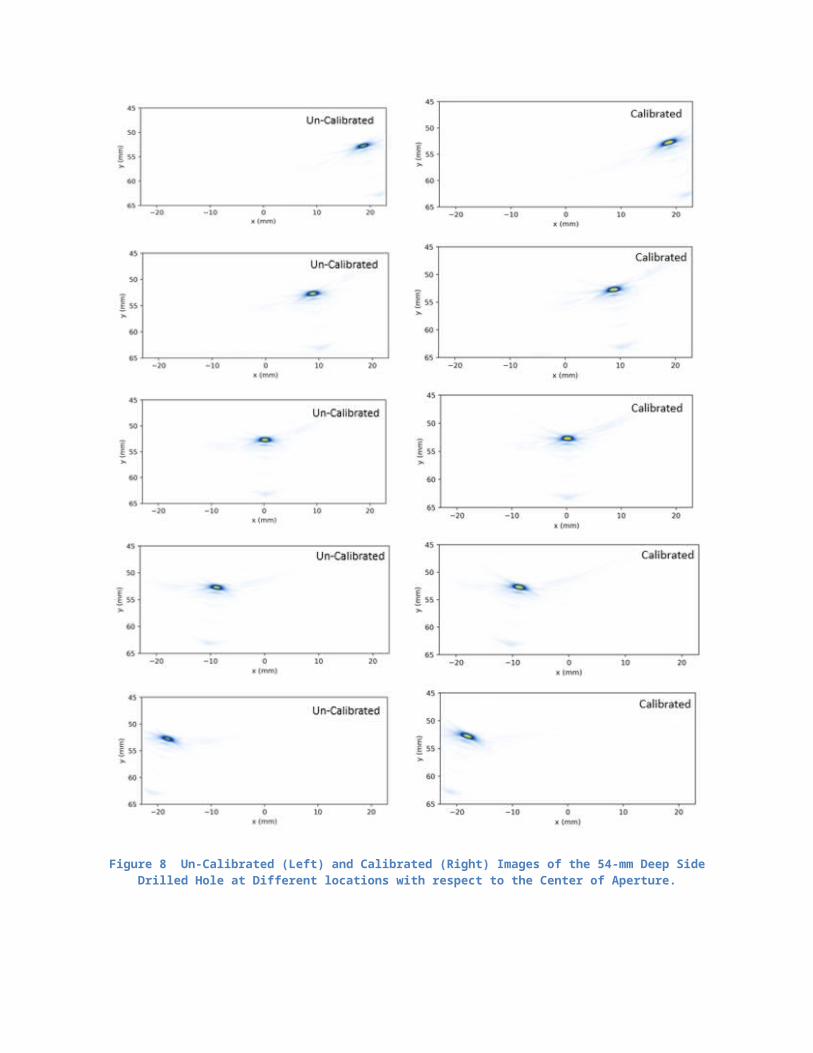
The effectiveness of the proposed amplitude correction procedure was evaluated by imaging 3 side drilled holes (2.5 mm diameter), at various depths and horizontal positions with respect to the center of the probe aperture. An Olympus 5L64-A2 probe (64 elements, 5 MHz center frequency, 0.6 mm pitch) was used for the calibration process. For each hole, FMC captures were recorded with the center of the aperture positioned -18.9 mm, -9.45 mm, 0 mm, 9.45 mm and 18.9 mm, with respect to the horizontal position of the target. Two TFM images were then rendered from each capture; first using the regular (uncorrected) method as described by equation 1 and then using the corrected method as described by equation 12. Figure 8 present rendered TFM images for side drilled hole with a depth of 54 mm. Un-Calibrated TFM images are presented in the left column and the Calibrated TFM images are presented in the right column on the images.

Figure 8 Un-Calibrated (Left) and Calibrated (Right) Images of the 54-mm Deep Side Drilled Hole at Different locations with respect to the Center of Aperture.

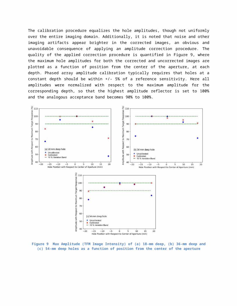
The calibration procedure equalizes the hole amplitudes, though not uniformly over the entire imaging domain. Additionally, it is noted that noise and other imaging artifacts appear brighter in the corrected images, an obvious and unavoidable consequence of applying an amplitude correction procedure. The quality of the applied correction procedure is quantified in Figure 9, where the maximum hole amplitudes for both the corrected and uncorrected images are plotted as a function of position from the center of the aperture, at each depth. Phased array amplitude calibration typically requires that holes at a constant depth should be within +/- 5% of a reference sensitivity. Here all amplitudes were normalized with respect to the maximum amplitude for the corresponding depth, so that the highest amplitude reflector is set to 100% and the analogous acceptance band becomes 90% to 100%.

Figure 9 Max Amplitude (TFM Image Intensity) of (a) 18-mm deep, (b) 36-mm deep and (c) 54-mm deep holes as a function of position from the center of the aperture

For the shallowest hole (18 mm depth), the corrected indication amplitude was observed to be within the Phased Array code accepted [5] 10% from maximum band, for the 3 holes closest to the center of the aperture ( Figure 9-a). For the 36 mm deep hole, the corrected indication amplitude was observed to be within a 10% tolerance for all positions (Figure 9-b). For the deepest hole (54 mm), the indication amplitude was observed to be within 10% of the maximum for all positions except for the hole located at -18 mm from the center of the aperture (Figure 9-c), with the measured amplitude being just below the acceptance threshold (89%). In general, the beam profile based calibration procedure seems to be more effective as the target depth increases. This is due, in part, to the fact that the difference in sound path between any 2 element pairs decreases for larger imaging depths. Nevertheless, the 10% variation in target amplitude for reflectors at a constant depth can only be met using the proposed beam profile correction scheme for targets imaged within ±10 mm of the center of the aperture, which amounts to only 53% of the total aperture length, though it is noted that only the shallowest target is out of tolerance. Clearly, the proposed procedure alone severely restricts the range for which a given probe can be acceptably calibrated based on the phased array code.

The TFM can be interpreted as synthetically point focusing at every pixel point within a chosen domain [1]. For points close to the aperture, an incredibly narrow, high intensity focus is achieved. For points far away from the aperture, the focal point becomes more spread out, with a lower maximum amplitude as shown in Figure 10. The spread of the synthetic focus is called a point spread function, and causes distortion of targets not well covered by the probe aperture; as observed in Figure 8, where the images of holes farthest from the center of the aperture appear increasingly elongated. The effects of imaging using a finite aperture cannot be neglected in correcting image amplitudes without significantly reducing the coverage range of a given phased array probe. In addition, the apparent distortion of targets near the edge of the aperture clearly implies that different sizing criteria will be required depending on where the target appears.

Figure 10 Effects of Focusing Away from the Center of the Aperture.

6. Conclusion

A simple procedure for estimating representative beam profiles for phased array probe elements was presented and used to equalize amplitudes across rendered TFM images. The proposed method has the advantage of estimating the amplitude corrections using measured A-scan data collected from a simple step block and does not rely on standard

mathematically expressions for element field profiles which neglect the effects of probe bandwidth and passive aperture size. The technique was shown to meet the standard Phased Array code requirement of having target amplitudes within 10% of one another across the imaging range, for targets at constant depth – though this could only be achieved on the shallowest hole when imaged within 20 mm (53%) of the center of the probe aperture. Failure to calibrate amplitudes across the entire range was attributed to the effects of imaging using a finite aperture, which causes targets away from the centerline of the probe to appear distorted and at lower amplitude. The spatially varying point spread function which is intrinsic to the TFM, will have to be directly accounted for when calibrating amplitude in images rendered with the TFM, otherwise the inspection range over which amplitude can be acceptably calibrated must be roughly limited to the center 50% of the aperture, even if all elements are used.

References

[1] A J. Hunter, B.W. Drinkwater, P. D. Wilcox, “The Wavenumber Algorithm for Full-Matrix Imaging Using and Ultrasonic Array,” NDT Int., vol. 39, no. 7, pp. 525– 541, 2006.

[2] A. Velichko, P. D. Wilcox, B.W. Drinkwater, “Array Imaging and Defect Characterization Using Post-processing Approaches,” Advances in Acoustic Microscopy and High Resolution Imaging, from Principles to Applications, Chapter 10. pp. 275– 318, 2013.

[3] B. W. Drinkwater and P. D. Wilcox, “Ultrasonic arrays for non- destructive evaluation: A review,” NDT Int., vol. 39, no. 7, pp. 525– 541, 2006.

[4] D. Cheeke, “Fundamentals and Applications of Ultrasonic Waves”, CRC Series in Pure and Applied Physics, 2002.

[5] ASME 2010, Section V T-464.1.3