Web Site: Email: [email protected] ...ijaiem.org/volume2issue9/IJAIEM-2013-09-29-076.pdfFig4 :BER...

International Journal of Application or Innovation in Engineering & Management (IJAIEM) Web Site: www.ijaiem.org Email: [email protected], [email protected]

Volume 2, Issue 9, September 2013 ISSN 2319 - 4847

Volume 2, Issue 9, September 2013 Page 275

Abstract Digital communication using MIMO has recently emerged as one of the most significant technical breakthrough in modern communications and also known as volume to volume wireless link. The effect of fading and interference always causes an issue for signal recovery in wireless communication This can be combated with application of an equalizer. Equalization compensates for Inter symbol Interference (ISI) created by multipath signal prorogation within time dispersive channels. In this paper we investigate the bit error rate performance characteristics of equalizers namely, ZF,SD,ML MMSE ,DFE, and MLSE equalizers. It also shows the relative burstiness of the errors, indicating that at low BERs, both the MLSE algorithm and the DFE algorithm suffer from error bursts. In particular, the DFE error performance is bustier with detected bits fed back than with correct bits fed back. Finally, during the "imperfect" MLSE portion of the simulation, it shows and dynamically updates the estimated channel response. The simulation results are obtained using Mat Lab tool box version 12. By the use of adaptive equalization to compensate for the time dispersion introduced by the channel Spurred by practical applications. Keywords: BER(Bit Error Rate),MIMO(Multiple Input Multiple Output),ZF(Zero Forcing),ISI(Inter Symbol Interference),ML(Maximum Likely hood),MMSE(Minimum Mean Square Error)DFE(Decision Feedback Equalizer) 1. INTRODUCTION The rising demand of multimedia services and the development of Internet related contents lead to increasing curiosity to high speed communications. In the ceaseless search for increased capacity in a wireless communication channel it has been shown that by using MIMO (Multiple Input Multiple Output) system architecture it is possible to increase that capacity considerably. The MIMO is very likely beneficial since it enables support of more antennas and larger bandwidths and it simplifies equalization in MIMO systems. Usually fading is considered as a problem in wireless communication but MIMO channels uses the fading to increase the capacity of entire system. Fading of the signal can be mitigated by different diversity techniques. The data rate and spectrum efficiency of wireless mobile communications have been significantly improved over the last decade or so. Recently, the advanced systems such as 3GPP LTE and terrestrial digital TV broadcasting have been sophisticatedly developed using OFDM and CDMA technology. In general, most mobile communication systems transmit bits of information in the radio space to the receiver. The radio channels in mobile radio systems are usually multipath fading channels, which cause inter-symbol interference (ISI) in the Received signal. To remove ISI from the signal, there is a need of strong equalizer which requires knowledge on the channel impulse response (CIR).[1]Hence, there is a need for the development of novel practical, low complexity equalization techniques and for understanding their potentials and limitations when used in wireless communication systems characterized by very high data rates, high mobility and the presence of multiple antennas.[10]In radio channels, a variety of adaptive equalizers can be used to cancel interference while providing diversity. Since the mobile fading channel is random and time varying, equalizers must track the time varying characteristics of the mobile channel, and thus are called adaptive equalizers. The general operating modes of an adaptive equalizer include training and tracking. First, a known, fixed-length training sequence is sent by the transmitter so that the receiver’s equalizer may adapt to a proper setting for minimum bit error rate (BER) detection. OVERVIEW OF MIMO- SYSTEM The MIMO system transmits different signals from each transmit element so that the receiving antenna array receives a superposition of all the transmitted signals. All signals are transmitted from all elements once and the receiver solves a linear equation system to demodulate the message. Multiplexing (MIMO) system is an effective solution to improve communication quality, performance, capacity, and transmission rate. MIMO is under intensive investigation by researchers

Fig-1 Transmit 2 Receive (2×2) MIMO

Improved Adaptive Bit Error Rate Performance for Fading Channel Communication

Pradyumna Ku. Mohapatra1, Siba Prasad Panigrahi2 ,Jibanananda Mishra3

1OEC,BPUT,BBSR

2CVRCE,BPUT,BBSR 3OEC,BPUT,BBSR



Volume 2, Issue 9, September 2013 76

We consider the system where the transmitter has antennas and the receiver has antennas. Let , be a complex number corresponding to the channel gain between transmit antenna n and the receive antenna m. If at a certain time instant complex signals are transmitted via the nt antennas, the received signals at antenna m can be expressed as

Where is a noise signal. This relation is easily expressed in a matrix structure. Let x and y be and nr vectors containing the transmitter and receiver data, respectively. Define the following channel gain matrix

H= (2)

Then we have, Where, Is a vector of noise sample 3. FLAT RAYLEIGH FADING MODEL The propagating radio signals are affected by the physical channel in various ways. To specify a situation of frequency-flat Rayleigh fading, a model is introduced called flat Rayleigh fading model. This is a reference model, Fast fading component has Rayleigh density function if there is no direct path from signalling parts. Rayleigh distribution is as follows,

3(A):BER SIMULATION OF BPSK IN A 10-TAP RAYLEIGH FADING CHANNEL : (a)Generation of random binary sequence.BPSK modulation i.e. bit 0 represented as -1 and bit 1 represented as +1 (b)Assigning to multiple OFDM symbols where data subcarriers from -26 to -1 and +1 to +26 are used, adding cyclic prefix, (c) Convolving each OFDM symbol with a 10-tap Rayleigh fading channel. The frequency response of fading channel on each symbol is computed and stored. (d)Concatenation of multiple symbols to form a long transmit sequence (e) Adding White Gaussian Noise. Grouping the received vector into multiple symbols, removing cyclic prefix (f)Counting the number of bit errors. Repeating for multiple values of .The simulation results are as shown in the plot below.

FIG 2:BER for BPSK using OFDM in a FIG:3 BER for BPSK in Rayleigh Channel 10-tap Rayleigh Channel 4. MINIMUM MEAN SQUARE ERROR (MMSE) In statistics and signal processing, a minimum mean square error (MMSE) estimator describes the approach which minimizes the mean square error (MSE), which is a common measure of estimator quality. Mathematically, Let be an unknown random variable, and let Y be a known random variable (the measurement). An estimator is any function of the measurement Y, and its MSE is given by Where the expectation is taken over both X and Y. The MMSE estimator is then defined as the estimator achieving minimal MSE. 4(A). MIMO WITH MMSE EQUALIZER In a 2×2 MIMO channel, probable usage of the available 2 transmit antennas can be as follows: 1. Consider that we have a transmission sequence, for example 2. In normal transmission, we will be sending x1 in the first time slot,x2 in the second time slot, and so on.




3. However, as we now have 2 transmit antennas, we may group the symbols into groups of two. In the first time slot, send x1andx2 from the first and second antenna. In second time slot, send x3 and x4 from the first and second antenna; send x5 and x6 in the third time slot and so on. 4. we are grouping two symbols and sending them in one time slot, we need only n/2 time slots to complete the transmission-data rate is doubled .This forms the simple explanation of a probable MIMO transmission scheme with 2 transmit antennas and 2 receive antennas 4(B).SIMULATION OF MIMO OFDM FOR COMPUTING MINIMUM MEAN SQUARE ERROR (MMSE) It is clearly seen from the simulation result of MIMO with MMSE without OFDM that, in increase SNR then Probability of error will get decrease. Now we want to find practically the results of MIMO with MMSE using OFDM how this will change the obtainable error From the following simulation results we find that the theoretical performance of Maximal Ratio Combining (MRC) diversity technique is best among all the receiver techniques. And there is a big difference of practical Performance of MMSE. The Synchronization factor in an OFDM system is the most critical one. When the receiver is initially turned on, it is not in synchronization with the transmitter. For this reason, data transmission in an OFDM System might need data to be sent in frames. At the beginning of each frame a null symbol is transmitted, so that the receiver can detect incoming data using simple envelope detection techniques. However, the noise in the signal might interfere with the envelope detection process. In general, it has been found that the receiver synchronizes itself with the transmitter in a time interval less than or equal to the guard interval. The Complexity of performing an FFT is dependent on the size of the FFT. However, it can be seen that because the symbol period increases with a larger FFT, the extra processing required is minimal. For e.g. the 2048-point FFT requires only 1.1 times the time required for processing a 1024-point FFT Now let us think about the other results of different MIMO strategies with MMSE receiver. What a great change we got in 2x3 MIMO with MMSE (without OFDM) as compared to the MRC. We achieved a difference of 1db between the MRC and MMSE. And the MMSE equalizer is now able to show better performance in comparison with MRC. Better results can be obtained if we increase size of the MIMO Simulation Model

(a) Generate Random binary sequence 1’s& -1’s (b) Group them into pair of symbols and send two symbols into one time slot (c) Multiply the symbol with the channel and then add white Gussian noise (d) Equalized the received symbols (e) Perform hard decision decoding and count bit errors (f) Repeat the multiple values of and plot the simulation and theoretical result

Fig4 :BER for BPSK with 2×2 MIMO&MMSE Fig 5:BER for BPSK with 2×2 MIMO&MMSE-SIC

5. Zero Forcing Equalizer Zero Forcing Equalizer is a linear equalization algorithm used in communication systems, which inverts the frequency response of the channel. This equalizer was first proposed by Robert Lucky. The Zero-Forcing Equalizer applies the inverse of the channel to the received signal, to restore the signal before the channel. The name Zero Forcing corresponds to bringing down the ISI to zero in a noise free case. This will be useful when ISI is significant compared to noise. For a channel with frequency response F(f) the zero forcing equalizer C(f) is constructed such that Thus the combination of channel and equalizer gives a flat frequency response and linear phase F(f)C(f) = 1.If the channel response for a particular channel is H(s) then the input signal is multiplied by the reciprocal of this. This is intended to remove the effect of channel from the received signal, in particular the Inter symbol Interference (ISI). let us consider a 2x2 MIMO channel, the Channel is modelled as, The received signal on the first receive antenna is,




Where are the received symbol on the first and second antenna respectively,

is the channel from 1st transmit antenna to 1st receive antenna, is the channel from 2nd transmit antenna to 1st receive antenna, is the channel from 1st transmit antenna to 2nd receive antenna, is the channel from 2nd transmit antenna to 2nd receive antenna,

are the transmitted symbols and are the noise on 1st and 2nd receive antennas.

The equation can be represented in matrix notation as follows = + (7)

Equivalently

To solve for x, we need to find a matrix W which satisfies WH = I. The Zero Forcing (ZF) detector for meeting this constraint is given by

Where W - Equalization Matrix and H - Channel Matrix This matrix is known as the Pseudo inverse for a general m x n matrix where

=

Note that the off diagonal elements in the matrix HHH are not zero, because the off diagonal elements are non zero in values. Zero forcing equalizer tries to null out the interfering terms when performing the equalization, i.e. when solving for x1 the interference from x2 is tried to be nulled and vice versa. While doing so, there can be an amplification of noise. Hence the Zero forcing equalizer is not the best possible equalizer. However, it is simple and reasonably easy to implement. For BPSK Modulation in Rayleigh fading channel, the BER is defined as

(11)

Where - Bit Error Rate

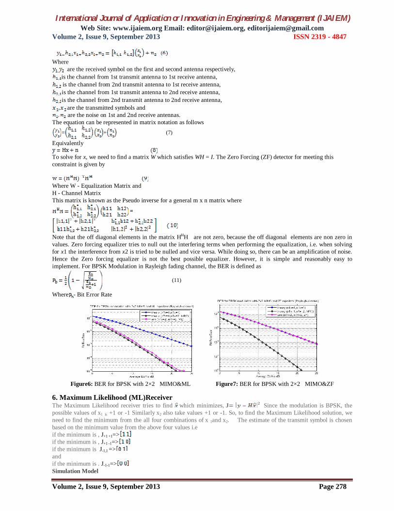
Figure6: BER for BPSK with 2×2 MIMO&ML Figure7: BER for BPSK with 2×2 MIMO&ZF

6. Maximum Likelihood (ML)Receiver The Maximum Likelihood receiver tries to find which minimizes, J 2 Since the modulation is BPSK, the possible values of x1 is +1 or -1 Similarly x2 also take values +1 or -1. So, to find the Maximum Likelihood solution, we need to find the minimum from the all four combinations of x 1and x2. The estimate of the transmit symbol is chosen based on the minimum value from the above four values i.e if the minimum is , J+1 +1=> if the minimum is , J+1 -1=> if the minimum is J-1,1 => and if the minimum is . J-1-1=> Simulation Model




(a)Generate Random binary sequence 1’s& -1’s (b)Group them into pair of symbols and send two symbols into one time slot (c)Multiply the symbol with the channel and then add white Gussian noise (d)Find the minimum four possible transmit symbol combinations (e)Based on the minimum chose the estimate of transmit symbol (f)Repeat the multiple values of and plot the simulation and theoretical result

7.CHANNEL EQUALIZATION ISI problem is resolved by channel equalization [12] in which the aim is to construct an equalizer such that the impulse response of the channel/equalizer combination is as close to as Possible , where Δ is a delay. Frequently the channel parameters are not known in advance and more over they may vary with time, in some applications significantly. Hence, it is necessary to use the adaptive equalizers, which provide the means of tracking the channel characteristics. The following figure shows a diagram of a channel equalization system.

Fig7. Digital transmission system using channel equalization

In the previous figure, s(n) is the signal that you transmit through the communication channel, and x(n) is the distorted output signal. To compensate for the signal distortion, the adaptive channel equalization system completes the following two modes: Training mode - This mode helps you determine the appropriate coefficients of the adaptive filter. When you transmit the signal s(n) to the communication channel, you also apply a delayed version of the same signal to the adaptive filter. In the previous figure, z-∆ is a delay function and d(n) is the delayed signal, y(n) is the output signal from the adaptive filter and e(n) is the error signal between d(n) and y(n) . The adaptive filter iteratively adjusts the coefficients to minimize e(n) After the power of e(n) converges, y(n) is almost identical to d(n) ,which means that you can use the resulting adaptive filter coefficients to compensate for the signal distortion. Decision-directed mode - After you determine the appropriate coefficients of the adaptive filter, you can switch the adaptive channel equalization system to decision-directed mode. In this mode, the adaptive channel equalization system decodes the signal and y(n) produces a new signal, which is an estimation of the signal s(n) except for a delay of Δ taps .Here, Adaptive filter plays an important role. The structure of the adaptive filter is showed in Fig.3

Fig 8. Adaptive filter

To start the discussion of the block diagram we take the following assumptions: The input signal is the sum of a desired signal d (n) and interfering noise v (n)

The variable filter has a Finite Impulse Response (FIR) structure. For such structures the impulse response is equal to the filter coefficients. The coefficients for a filter order p are defined as

the error signal or cost function is the difference between the desired and the estimated signal

The variable filter estimates the desired signal by convolving the input signal with the impulse response. In vector notation this is expressed

Where

is an input signal vector. Moreover, the variable filter updates the filter coefficients at every time instant




Where is a correction factor for the filter coefficients .The adaptive algorithm generates this correction factor based on the input and error signals 8. ADAPTATION ALGORITHMS This section briefly introduces two well-known algorithms that possess different qualities in terms of the performance i.e one is least mean square (LMS) and other is Recursive least square filter (RLS). A. Least Mean Squares Algorithm (LMS) The least mean-square (LMS) algorithm is probably the most widely used adaptive filtering algorithm, being employed in several communications systems. It has gained popularity due to its low computational complexity and proven robustness. The LMS algorithm is a gradient-type algorithm that updates the coefficient vector by taking a step in the direction of the negative gradient [12] of the objective function, i.e.,

Table 1.1: The Least Mean Square Algorithm

LMS ALGORITHM for each k {

} where μ is the step size controlling the stability, convergence speed, and misadjustment. To find an estimate of the gradient, the LMS algorithm uses as objective function the instantaneous estimate of the MSE, i.e resulting

in the gradient estimate

The pseudo-code for the LMS algorithm is shown in Table 1.1. In order to guarantee stability in the mean-squared sense, the step size μ should be chosen in the range where tr{.} is the trace operator and

is the input-signal autocorrelation matrix. The upper bound should be considered optimistic and in practice a smaller value is recommended [1]. A normalized version of the LMS algorithm, the NLMS algorithm [6], is obtained by substituting the step size in Equation (1.4) with the time-varying step size where The NLMS algorithm is in the control literature referred to as the projection algorithm (PA) The main drawback of the LMS and the NLMS algorithms is the slow convergence for colored noise input signals. In cases where the convergence speed of the LMS algorithm is not satisfying, the adaptation algorithms presented in the following sections may serve as viable alternatives.

Table 1.2: The Recursive Least Square Algorithm RLS ALGORITHM

(I) ,δ Small positive constant for each k { K(k) =

R(K)=

]

]

}




B.The Recursive Least-Squares (RLS) Algorithm Convergence of the LMS algorithm operating in colored environment, one can implement the recursive least-squares (RLS) algorithm [6, 10]. The RLS algorithm is a recursive implementation of To overcome the problem of slow the least-squares (LS) solution, i.e., it Minimizes the LS objective function. The recursions for the most common version of the RLS algorithm, which is presented in its standard form in Table 1.2, is a result of the weighted least-squares (WLS) objective function

) Differentiating the objective function with respect to w(k) and solving for the minimum yields the following equations

(i)]w(k)= ) Where 0 < λ ≤ 1 is an exponential scaling factor often referred to as the forgetting factor. Defining the quantities

and = the solution is obtained as (k) (25) The recursive implementations is a result of the formulations

And

The inverse R−1(k) can be obtained recursively in terms of R−1(k−1) using the matrix inversion lemma1 [10] thus avoiding direct inversion of R(k) at each time instant k. The main problems with the RLS algorithm are potential divergence behavior in finite-precision environment and high computational complexity, which is of order N2 9. Adaptive Equalization Technique Different kinds of Equalizer are available in the text like Fractionally Spaced Equalizer, Blind Equalization, Decision- Feedback Equalization, Linear Phase Equalizer, T-Shaped Equalizer, Dual Mode Equalizer and Symbol spaced Equalizer. But most widely used equalizers are discussed as follow: A. Decision-Feedback Equalization The basic limitation of a linear equalizer, such as transversal filter, is the poor perform on the channel having spectral nulls. A decision feedback equalizer (DFE) is a nonlinear equalizer that uses previous detector decision to eliminate the ISI on pulses that are currently being demodulated. In other words, the distortion on a current pulse that was caused by previous pulses is subtracted. Figure 7 shows a simplified block diagram of a DFE where the forward filter and the feedback filter can each be a linear filter, such as transversal filter. The nonlinearity of the DFE stems from the nonlinear characteristic of the detector that provides an input to the feedback filter. The basic idea of a DFE is that if the values of the symbols previously detected are known, then ISI contributed by these symbols can be cancelled out exactly at the output of the forward filter by subtracting past symbol values with appropriate weighting. The forward and feedback tap weights can be adjusted simultaneously to fulfil a criterion such as minimizing the MSE. The DFE structure is particularly useful for equalization of channels with severe amplitude distortion, and is also less sensitive to sampling phase offset.

Figure9. Decision feedback equalizer 10. Simulation of DFE&MLSE channel equalizer This example constructs and implements a linear equalizer object and a decision feedback equalizer (DFE) object. It also initializes and invokes maximum likelihood sequence estimation (MLSE) equalizer. The MLSE equalizer is first invoked with perfect channel knowledge, then with a straight forward but imperfect channel estimation technique.As the simulation progresses, it updates a BER plot for comparative analysis between the equalization methods. It also shows the signal spectra of the linearly equalized and DFE equalized signals. It also shows the relative burstiness of the errors,




indicating that at low BERs, both the MLSE algorithm and the DFE algorithm suffer from error bursts. In particular, the DFE error performance is bustier with detected bits fed back than with correct bits fed back. Finally, during the "imperfect" MLSE portion of the simulation, it shows and dynamically updates the estimated channel response. A.SIMULATION MODEL FOR DFE (a)Set parameters related to the signal and channel (b). Use BPSK without any pulse shaping, and a 5-tap real-valued symmetric channel impulse response (c) Set parameter values for the linear and DFE equalizers. (d) Use a 31-tap linear equalizer, and a DFE with 15 feed forward and feedback taps. (e) Use the recursive least squares (RLS) algorithm for the first block of data to ensure rapid tap convergence. (f) Use the least mean square (LMS) algorithm thereafter to ensure rapid execution speed. B.SIMULATION MODEL FOR MLSE (a) Set the parameters of the MLSE equalizer. (b) Use a trace back length of six times the length of the channel impulse response. (c) . Initialize the equalizer states. (d) Set the equalization mode to "continuous", to enable seamless equalization over multiple blocks of data. (e) Use a cyclic prefix in the channel estimation technique, and set the length of the prefix. Assume that the estimated length of the channel impulse response is one sample longer than the actual length.




11. Conclusion: In this paper we investigate the bit error rate performance characteristics of equalizers namely, ZF,SD, ML, MMSE ,DFE, and MLSE equalizers. It also shows the relative burstiness of the errors, indicating that at low BERs, both the MLSE algorithm and the DFE algorithm suffer from error bursts. In particular, the DFE error performance is bustier with detected bits fed back than with correct bits fed back. Finally, during the "imperfect" MLSE portion of the simulation, it dynamically updates the estimated channel response. References: [1] X. Zhu and R. D Murch,Layeredspace frequency equalization in a single-carrier MIMO system for frequency-

selective channels, IEEE Trans. Wireless Commun., vol. 3, no. 3, pp. 701–708, (May 2004) [2] Krishna Sankar, “BER for BPSK in OFDM with Rayleigh multipath channel” on August 26, 2008 [3] G. Leus, S. Zhou, and G. B. Giannakis, “Orthogonal multiple access over time- and frequency-selective channels,”

IEEE Transactions on Information Theory, vol. 49, no. 8, pp. 1942–1950, 2003. [4] Kyung Won Park and Yong Soo Cho,"An MIMO OFDM technique for high-speed mobile channels," IEEE

Communications Letters, Volume 9, No. 7, PP. 604 – 606(July 2005). [5] T. S. Rappaport, “Wireless Communications: Principles and Practice”, Second Edition, 2002 [6] J. G. Proakis, “Digital Communications”, Fourth Edition, 2001




[7] S. Haykin, “Adaptive Filter Theory”, Fourth Edition, 2002 [8] “ZERO-FORCING EQUALIZATION FOR TIME-VARYING SYSTEMS WITH MEMORY “ by Cassio B. Ribeiro,

Marcello L. R. de Campos, and Paulo S. R. Diniz. [9] N.Sathish Kumar and Dr .K.R.Shankar umar,2011.“Performance Analysis of M X N Equalizer Based Minimum

Mean Square Error (MMSE) Receiver for MIMO Wireless Channel”International Journal of Computer Applications 16(7):47– 50, doi:10.5120/2021-2726.

[10] S.Nagarani C.V.Seshiah,2011. “An Efficient Space-Time-Coding for Wireless Communication”. European Journal of Scientific Research Vol.52 No.2 pp.195-203.

[11] P. S. R. Diniz, Adaptive Filtering: Algorithms and Practical Implementations, Kluwer Academic Publishers, Boston, 1997.

[12] B. Widrow and M. E. Hoff, “Adaptive switching circuits,” IRE Western Electric Show and Convention Record, pp. 96–104, August 1960

[13] Adinoyi, S. Al-Semari, A. Zerquine, “Decision feedback equalisation of coded I-Q QPSK in mobile radio environments,” Electron. Lett. vol. 35,No1, pp. 13-14, Jan. 1999.

[14] Wang Junfeng, Zhang Bo, “Design of Adaptive Equalizer Based on Variable Step LMS Algorithm,” Proceedings of the Third International Symposium on Computer Science and Computational Technology(ISCSCT ’10) Jiaozuo, P. R.China, 14-15, pp. 256-258,August 2010

[15] Antoinette Beasley and Arlene Cole-Rhodes, “Performance of Adaptive Equalizer for QAM signals,” IEEE, Military communications Conference, 2005. MILCOM 2005, Vol.4, pp. 2373 - 2377

[16] Mahmood Farhan Mosleh, Aseel Hameed AL-Nakkash, “Combination of LMS and RLS Adaptive Equalizer for Selective Fading Channel,” European Journal of Scientific Research ISSN 1450-216X Vol.43, No.1,pp.127-137, 2010.

Web Site: Email: [email protected] ...ijaiem.org/volume2issue9/IJAIEM-2013-09-29-076.pdfFig4 :BER...

Documents

Transcript of Web Site: Email: [email protected] ...ijaiem.org/volume2issue9/IJAIEM-2013-09-29-076.pdfFig4 :BER...