Web Note 9 State Fiscal Model FINAL - UAA Institute of

of 13

Revising the State Fiscal Plan to Account for Petroleum Wealth

by Scott Goldsmith Web Note No. 9

May 2011

INTRODUCTION In 2008 the Alaska Legislature passed and the governor signed into law a bill requiring the Office of Management and Budget (OMB) to prepare an annual state fiscal plan projecting state spending for 10 years and identifying the revenue sources to pay for that spending. One objective of the law was to get government and the general public thinking, discussing, and planning for the long-term fiscal health of the state in light of declining oil production. These plans have not attracted the attention they deserve. In this Web Note we review the most recent fiscal year 2012 10-year plan and offer suggestions for improvement. THE OMB FISCAL YEAR 2012 10-YEAR FISCAL PLAN The fiscal plan consists of a number of scenarios, based on different assumptions about future petroleum revenues and the growth rate of General Fund spending. Each scenario tracks the BUDGET SURPLUS/SHORTFALL (difference between current revenues and expenditures) as well as TOTAL RESERVES (balance in the Constitutional and Statutory Budget Reserves). For example, “Scenario 3,” depicted in the table and figure below, shows TOTAL RESERVES growing from $11.1 billion in FY11 to $19.6 billion in FY21, based on the Fall 2010 Alaska Department of Revenue forecast of General Fund revenues and a 6% growth rate in General Fund expenses.

This paper is part of ISER’s Investing for Alaska’s Future research initiative, funded by a grant from Northrim Bank.

INSTITUTE OF SOCIAL AND ECONOMIC RESEARCH UNIVERSITY OF ALASKA ANCHORAGE

May 2011 Web Note 9 of 13

Based on those assumptions, the state would enjoy a BUDGET SURPLUS through FY18, but growing annual expenses (the vertical bars below) would then begin to exceed revenues (solid line). An annual SHORTFALL would appear and start to grow.

The BUDGET SHORTFALL occurs as soon as FY12 in the most pessimistic of the five fiscal plan scenarios but does not show up at all before FY21 in the two most optimistic of the scenarios (table below). The extreme sensitivity of state fiscal health to the growth rate of spending and future petroleum revenues is also illustrated by comparing TOTAL RESERVES in FY21 across the five scenarios. They vary from zero to $36.9 billion.

Table 1. Summary of 5 OMB Scenarios: BUDGET SHORTFALL and TOTAL RESERVES

Scenario GF Revenues GF Expenditure Growth Rate (Nominal $)1

Year of First BUDGET

SHORTFALL

TOTAL RESERVES in 2021 (Billion$)

1 DOR Fall 2010 0% - $36.9 2 DOR Fall 2010 3% - $28.9 3 DOR Fall 2010 6% 2019 $19.6 4 $80 constant oil 3% 2013 $3.1 5 $70 constant oil 1% 2012 -

The state fiscal plan reflected in these scenarios is built on several elements:

• Contain growth in state spending • Encourage oil and gas development to realize the projected revenue stream

1 The fiscal plan is presented in nominal dollars and assumes inflation at 2.75% annually and population growth of 1% annually. So the General Fund expenditure growth rates in Scenarios 1 and 2 are negative or flat in inflation-adjusted dollars. This will be very difficult to achieve. For example, state Medicaid expenditures, one of the largest items in the budget, have been projected to grow at 8.9% annually. See Long-Term Forecast of Medicaid Enrollment and Spending in Alaska: 2005-2025, by the Lewin Group and ECONorthwest, 2006.



• Save all current account budget surpluses in the CBRF (Constitutional Budget Reserve) or other account

• Use accumulated surpluses to cover unanticipated revenue shortfalls or general fund expenses

• Continue Permanent Fund dividend appropriation using current formula2 • Reduce spending if accumulated surplus gets low or becomes depleted • No new taxes

These plan elements are designed to ensure that public services can be provided, the economy can continue to prosper, and no fiscal burden will be passed on to the next generation of Alaskans in the form of new taxes or service cuts. But can it work? If revenues are high and spending growth is slow, this plan should work for the next decade. And the higher than anticipated oil price in recent months has provided the state with an additional cushion to help ensure its success. LOOKING BEYOND 10 YEARS The problem with this approach is that petroleum revenues, which pay for at least 90% of General Fund spending, are non-sustainable. Eventually, even under the most optimistic assumptions, growing General Fund spending will overtake falling General Fund revenues from oil, the annual draw on reserves will increase, and TOTAL RESERVES will not only fall, they will disappear. To avoid this problem, the fiscal plan suggests revenues from North Slope natural gas production after 2020 will be a “key element in providing for the future fiscal and economic stability of the state”3 but there is no quantitative analysis to support that statement. Let’s extend OMB Scenario 3 for 10 years, out to FY32, and look at the results graphically. We assume General Fund spending (black line) continues to grow at 6% a year through FY32, nominal General Fund oil revenue after FY21 falls 5% annually (green area), and other revenues (red) grow 3% annually. The graph also shows spending from RESERVES (yellow). Gas revenues, based on an estimated wellhead value of $2 and the current tax structure, (blue) start in FY21. The projections are shown in inflation-adjusted dollars to allow comparisons of future and current values.4 We see that gas revenues reduce but are not large enough to eliminate the General Fund SHORTFALL. Gas revenues allow the size of the financial RESERVE to stay above $20 billion for several years, but eventually the force of growing expenditures and declining petroleum

2 This element is not explicitly stated. Neither is the implied assumption that the Earnings Reserve of the Permanent Fund will not be available for appropriation for General Fund spending. In what follows we assume use of the Earnings Reserve to help fund the General Fund. 3 OMB FY2012 10-Year Plan, Executive Summary, page 1. 4 These projections are based on a simple spreadsheet model available from the author.



revenues leads to its rapid depletion through annual withdrawals (yellow). By FY32 the financial RESERVE is gone. By that time the annual SHORTFALL has grown to about $5 billion.

OMB FISCAL PLAN—EXTENDED (2012 Billion $) GF Projection Financial Reserve Balance

A SHORTFALL of $5 billion would not only devastate public spending—for education, health care, public safety, transportation, and other purposes—it would also have a ripple effect on the entire economy, resulting in a severe and long lasting recession. The prolonged recession of the mid-1980s demonstrated how sensitive the economy is to public spending and how every part of the economy suffers when government spending falls sharply. The lesson from looking beyond this decade is that gas revenues could postpone depletion of petroleum revenues, but could not eliminate the underlying problem of non-sustainability and the fiscal gap. DOWNSIDE RISK What if the future does not look as the OMB Fiscal Plan describes? The economic history of Alaska has been punctuated by pleasant surprises—like the discovery of oil at Prudhoe Bay, the oil price increase due to the Iran-Iraq war shortly after Prudhoe Bay production began, and the more recent positive oil price trend. But we need only remember the severe recession of the mid-1980s, brought about when Saudi Arabia increased oil production and drove down the price, to realize that unpleasant surprises also can and have happened. We should consider a broader range of different possible futures and how the fiscal plan would work under those conditions. One possibility is that things will turn out better than anticipated in the OMB projection. Oil and gas revenues could end up higher than we expect. State spending could grow more slowly than projected. Under those circumstances, the reserve balance would grow more rapidly and we would be in the fortunate circumstance of having more money in the bank than expected. That outcome would be good in the near term, but with continued and growing dependence on a non-sustainable revenue source, the fiscal gap, when it appeared, could be even bigger than $5



billion. On the other hand, a delay or smaller revenues from gas commercialization; lower revenues from oil; or more rapid growth in General Fund expenditures could all have serious consequences for the fiscal future of the state within a few years. The next set of graphs shows what would happen if there were no revenues from gas. With declining General Fund oil revenues (green), the budget SHORTFALL that opens after FY18 grows and is filled using RESERVES (yellow) until they are gone in FY28. By that time the General Fund SHORTFALL has grown to more than $4 billion.5

OMB FISCAL PLAN—EXTENDED (2012 Billion $) NO GASLINE

GF Projection Financial Reserve Balance

If oil revenues turn out to be 75% of the DOR Fall 2010 projection, the budget SHORTFALL begins immediately and the financial RESERVE is depleted in FY23.


75% OF DOR OIL REVENUES GF Projection Financial Reserve Balance

5 Reserves used after FY28 shown in the graphs come from the portion of Permanent Fund earnings that are not used to pay the dividend or inflation proof the fund. That portion goes into the Earnings Reserve account of the Permanent Fund and is spent in the same year.



CLOSING THE FISCAL GAP

If commercialization of gas is delayed or oil revenues fall below current projections, we should be able to anticipate the need for corrective action to avoid huge budget SHORTFALLS. Three obvious possibilities are to cut spending, impose taxes, and divert the Permanent Fund dividend to the General Fund. Use of the Permanent Fund balance is a more drastic alternative.

a. Cut Spending Holding General Fund spending (black line) constant in real terms after FY20 (3% annual growth) has little immediate effect, but it does marginally reduce the fiscal gap in later years.


75% OF DOR OIL REVENUES CUT SPENDING AFTER 2020


b. Personal Taxes Alaska is the only state without either a state sales tax or personal income tax. Nationally, households contribute on average about 4% of their income to the operation of state government through a combination of these taxes. If Alaska households supported state government at the same rate as households in other states, personal tax collections would be about $1,800 per capita—4% of personal income. If these taxes were imposed (shown in purple on the graphs on the following page)6 before the financial reserves were depleted, it would postpone the arrival of the fiscal gap and cut down its size. The political challenge with this strategy is to collect tax revenues at the same time that the RESERVE holds several billion dollars.

6 The estimate is based on an analysis by the Urban Institute-Brookings Institution Tax Policy Center of data from the U.S. census. In 2007 tax revenue from state income and sales taxes averaged 4.25% of personal income for the U.S. as a whole. It ranged from a low of 2.33% in Texas to a high of 7.88% in Hawaii. Applying the U.S. average rate to 2008 Alaska personal income of $30 billion results in an estimate of about $1.3 billion in tax revenue. Sales tax revenue would be about $600 million, and the personal income tax revenue would be about $700 million.



OMB FISCAL PLAN—EXTENDED (2012 Billion $)

NO GASLINE 75% OF DOR OIL REVENUES CUT SPENDING AFTER 2020

ADD PERSONAL TAXES IN 2018


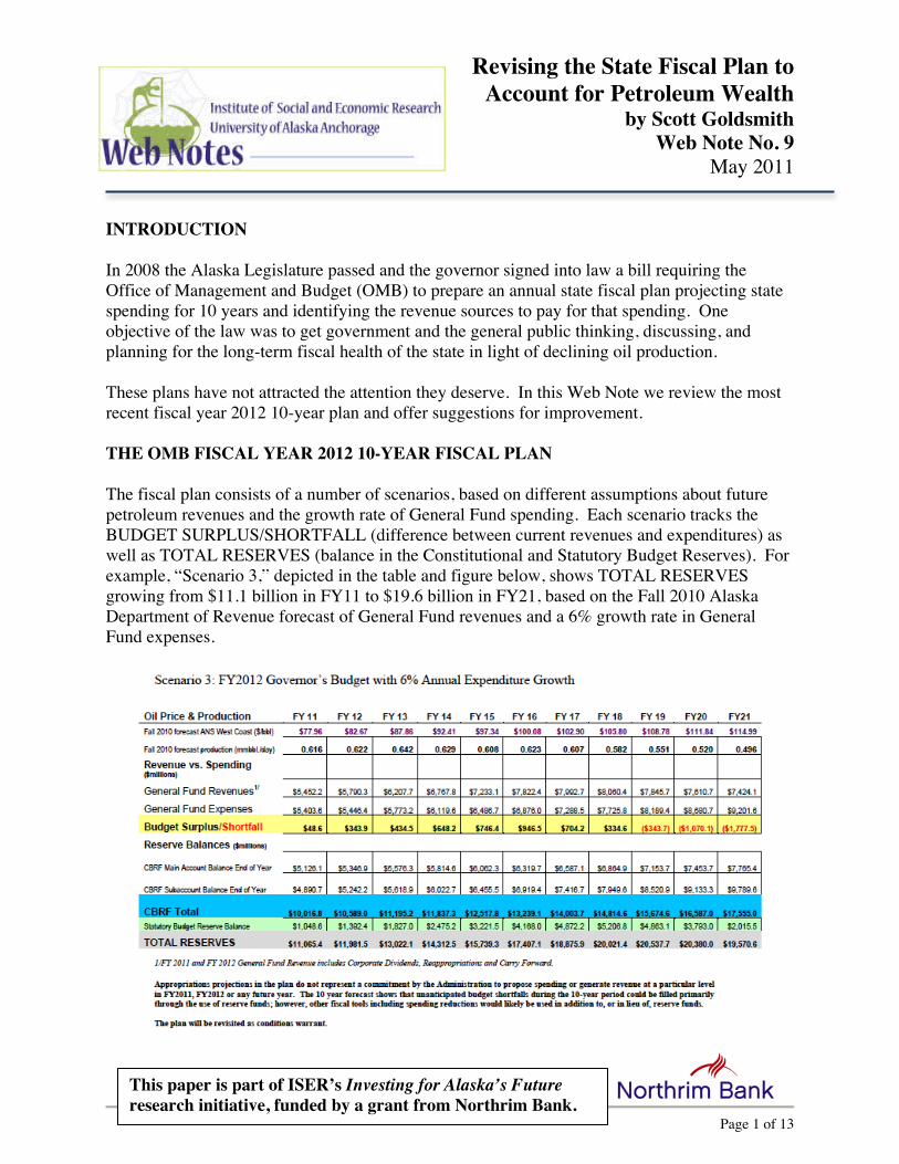
c. Divert the Permanent Fund Dividend to General Fund Diverting the entire dividend (red on the graph below) and adding personal tax revenues (purple) to cover General Fund spending would reduce the budget SHORTFALL and maintain the RESERVE (yellow) beyond FY32. But even in this case, after 20 years the RESERVE would soon be depleted because of the non-sustainability of the oil revenues.


75% OF DOR OIL REVENUES CUT SPENDING AFTER 2020

ADD PERSONAL TAXES IN 2018 DIVERT THE DIVIDEND TO THE GF IN 2022




d. Cash Out the Permanent Fund Using the Permanent Fund balance to fill the budget gap would work for a number of years, but like petroleum revenues, the fund is a non-sustainable revenue source and would not provide a permanent solution to the fiscal dilemma the state faces. FISCAL BURDEN Looking out 20 years forces us to confront the fiscal reality that the state continues to depend on non-renewable revenues to fund government and to support the state economy. Sooner or later spending will outrun available revenues. When that happens Alaskans will have to make do with less and pay more for what they get. Either way Alaskans at that time will bear a FISCAL BURDEN compared to the current generation. The only way to minimize that burden is to save more current revenues from non-renewable petroleum production, but how can we decide how much saving is enough? WEALTH PRESERVATION: THE MAXIMUM SUSTAINABLE YIELD If we are serious about being able to fund necessary public services in the future without imposing a FISCAL BURDEN on future generations, we should save enough out of current revenues from non-renewable sources to maintain the real per capita value of our wealth. But because current petroleum revenues fluctuate from year to year, it is easier to turn the question on its head and ask not how much we need to save, but rather how much we can afford to spend to maintain the per person value of our wealth. To do that we need to know the size of our petroleum wealth, including both the financial assets derived from past petroleum revenues and the value of petroleum still in the ground—the present value of future petroleum revenues. We estimate the state’s petroleum wealth as of June 30, 2010 (the beginning of fiscal year 2011) to have a value of $126 billion7—$45 billion held as financial assets (Table 2) and $81 billion as the present value of revenues yet to be collected from future oil and gas production (Table 3). This estimate of future revenues relies primarily on the Fall 2010 Alaska Department of Revenue projection.

7 See ISER Webnote No. 7, “How Much Should Alaska Save?” available at www.iser.uaa.alaska.edu for more detail on this method of determining petroleum wealth.



Table 2. State Financial Assets as of June 30, 2010 (Billion $) TOTAL $45

Permanent Fund $33.3 Alaska Permanent Fund Corporation, 2010 Annual Financial Report

Constitutional Budget Reserve

$8.7 Alaska Department of Revenue, Treasury Division, Combined Schedule of Invested Assets, June 30, 2010

Statutory Budget Reserve $1 Alaska Department of Revenue, Tax Division, Revenue Sources, Fall 2009

General Fund $2 Author estimate Other ‐

Source: ISER Web Note 7, How Much Should Alaska Save? Note: Cash in the General Fund is a rough measure of the share of the General Fund that is not in restricted accounts (of which the Statutory Budget Reserve is one) and is not necessary to meet the cash flow requirements of the state. For completeness we show an “Other” category, which would consist of other unrestricted financial assets that could be appropriated to support state spending.

Table 3. Present Value of State Petroleum Revenues Yet to be Collected (Billion $)

Total Petroleum $81 Oil $74 State Land—North Slope 2011‐2020 $45 State Land—North Slope 2021+ $27 State Land—Other Locations ‐ State Land—Heavy Oil $1 Federal NPRA ‐ Federal OCS $1 Federal ANWR ‐ Gas $7 Source: ISER Web Note 7, How Much Should Alaska Save? Author estimate, based largely on Alaska Department of Revenue projections. Future revenues discounted at 5% real. Includes royalties paid into Permanent Fund.

A wealth portfolio of $126 billion should be able to generate annual earnings, after inflation, of $6.3 billion if it can achieve a real rate of return of 5%—the target earnings for the Alaska Permanent Fund. With a stable state population, we could spend the entire earnings of $6.3 billion each year and still maintain the value of our wealth for future generations to share. But since the population is increasing about 1% annually, we would need to reinvest 1% of the earnings back into the portfolio in order to maintain per capita value. Then the wealth portfolio would be growing over time at the same rate as population.8 After that reinvestment the MAXIMUM SUSTAINABLE YIELD from the portfolio would be $5.04 billion.9 The calculation is shown in Table 4.

8 This is a simple version of what is known to economists as the Hartwick rule. 9 It could also be called the BENCHMARK DRAW.



Table 4. MAXIMUM SUSTAINABLE YIELD: FY 2011 (Billion $)

PETROLEUM WEALTH $ 126 Real Earnings @ 5% $ 6.30 Reinvest for Population Growth @ 1% $ 1.26 MAXIMUM SUSTAINABLE YIELD $ 5.04

Over time, the MAXIMUM SUSTAINABLE YIELD would need to grow with the population, keeping real per capita yield constant at the current level of $7,100, based on a population of 710 thousand.) The MAXIMUM SUSTAINABLE YIELD is the annual amount that could be spent for all purposes—government programs and the Permanent Fund dividend—from the entire petroleum wealth portfolio, including current petroleum revenues and earnings on all financial assets. REVISING THE FISCAL PLAN TO TRACK WEALTH PRESERVATION If we incorporated the objective of wealth preservation into the state fiscal plan, the sum of spending from three sources could not exceed the MAXIMUM SUSTAINABLE YIELD. These sources would be spending from the Permanent Fund, spending from other financial assets, and spending from current petroleum revenues. Revenues from recurring sources would fill any shortfall between total spending and the MAXIMUM SUSTAINABLE YIELD. The fiscal plan would look like the next set of graphs, which assume 6% annual growth in General Fund spending (black line) and continuation of the current policies regarding the Permanent Fund and payment of the dividend. The MAXIMUM SUSTAINABLE YIELD remaining after paying the dividend becomes income to the General Fund, shown in green. The difference between current General Fund spending and revenue from the MAXIMUM SUSTAINABLE YIELD (blue area) must come from recurring revenue sources.10

REVISED OMB FISCAL PLAN (2012 Billion $) GF Projection Petroleum Wealth Balance

10 The small red bar at the bottom is current non-petroleum General Fund revenue.



The entire petroleum wealth of the state is shown at the right; it includes all financial assets as well as the expected revenues from future petroleum production. The wealth grows over time through reinvestment of earnings at the same rate as population growth. The MAXIMUM SUSTAINABLE YIELD is the row of small yellow bars. Adhering to this plan would ensure that petroleum wealth would be shared across generations and that the cost of spending on public programs above the MAXIMUM SUSTAINABLE YIELD level would be borne by those who benefit from that spending.11 MONITORING HOW WE’RE DOING We can monitor how we’re doing in meeting the objective of wealth preservation—without redoing the state fiscal plan—by comparing actual spending from wealth in the state fiscal plan to the MAXIMUM SUSTAINABLE YIELD level of spending. If we are spending more, then our wealth per capita is falling. If we are spending less, our wealth per capita is growing. Table 5 shows estimated actual spending from petroleum wealth in FY12 to be about $6.1 billion. This consists of the General Fund oil revenues that will be spent, the General Fund investment earnings that will be spent, and the Permanent Fund Dividend.12

Table 5. FY2012 PROJECTED PETROLEUM WEALTH SPENDING (Billion $) TOTAL $ 6.057 GF Oil Revenues $ 4.648 Minus: GF Oil Revenues Saved (Budget Surplus) ($ .094) Plus: GF Investment Earnings $ .183 General Fund $4.737 Permanent Fund Dividend* $ 1.320 Based on FY 2011 10‐Year Fiscal Projection *Author Estimate for CY 2011 Distribution

Estimated actual spending exceeds the MAXIMUM SUSTAINABLE YIELD by about $1.1 billion (Table 6). This is the amount by which our petroleum wealth is falling and also the amount of the FISCAL BURDEN passed on to future generations.

Table 6. Tracking FY2012 Wealth Preservation Performance (Billion $) PROJECTED ACTUAL DRAW $6.1 MAXIMUM SUSTAINABLE YIELD $5.0 EROSION OF WEALTH $ 1.1

Because of the erosion of wealth, the MAXIMUM SUSTAINANABLE YIELD would be smaller next year. The decline would be small, but if the annual draws continued to exceed the

11 In this way it is like the Norwegian fiscal model which consciously attempts to balance current and future generation needs. 12 The actual draw will not be known until the end of the fiscal year.



MAXIMUM SUSTAINABLE YIELD the erosion of wealth would continue at an increasing rate. This can be seen in the next two graphs. The first shows the diverging paths of real per capita spending (rising)13 and real per capita MAXIMUM SUSTAINABLE YIELD (falling). The gap each year (left-hand graph) is the growing FISCAL BURDEN. The second graph shows real per capita petroleum wealth, declining over time.

FY2011 OMB 10-YEAR FISCAL PROJECTION (2012$) MONITORING WEALTH PRESERVATION (Thousand $)

Actual vs MSY Spending Per Capita Petroleum Wealth Per Capita

FACTORING IN UNCERTAINTY AND CHANGING CONDITIONS The MAXIMUM SUSTAINABLE YIELD can only be a general guideline for sustainability, because it will constantly change due to new forecasts of future petroleum revenues,14 variations in the rate of population growth, or changes in the discount rate. But because we have some idea of the range within which these variables are likely to fall, the idea of MAXIMUM SUSTAINABLE YIELD can still help inform state fiscal policy. Based on this knowledge we can estimate that the current range for the MAXIMUM SUSTAINABLE YIELD is about $1 billion below and $1 billion above the point estimate of $5 billion. The next figure shows that MAXIMUM SUSTAINABLE YIELD is not particularly sensitive to variations in the estimate of future petroleum revenues. The sloping lines indicate MAXIMUM SUSTAINABLE YIELD for different levels of estimated future petroleum revenues and rates of population growth. The lowest line, based on population growth of 1% annually, shows that if petroleum revenues have a value of $81 billion—our current estimate—the MAXIMUM SUSTAINABLE YIELD is $5 billion. The value of future petroleum revenues would need to be more than $105 billion before the MAXIMUM SUSTAINABLE YIELD increased to $6 billion. That would still be less than current spending from petroleum wealth.15

13 The line drops off when the financial assets have all been spent. 14 We know the exact value of petroleum wealth held as financial assets at any given time. 15 For example, based on the current market value of the Permanent Fund and the Spring 2011 Department of Revenue forecast, our petroleum wealth portfolio would be about $136 billion, consisting of $50 billion in financial assets and $86 billion in petroleum revenues not yet collected. The MAXIMUM SUSTAINABLE YIELD from a portfolio with that value would be $5.4 billion. The large change in estimated value of the petroleum wealth portfolio has a small impact on the size of the MAXIMUM SUSTAINABLE YIELD.



The other lines in the graph represent cases of zero population growth or negative population growth. MAXIMUM SUSTAINABLE YIELD would be significantly more if we think there will be fewer Alaskans in the future.

MAXIMUM SUSTAINABLE YIELD (2012) AS A FUNCTION OF PETROLEUM IN THE GROUND AND POPULATION GROWTH (BILLION $)

The next graph shows how the MAXIMUM SUSTAINABLE YIELD varies depending on the discount rate used to calculate the present value of future petroleum revenues and the rate of return on financial assets. At 5% the MAXIMUM SUSTAINABLE YIELD is $5 billion, but it is higher at higher discount rates and lower if the discount rate is lower.

MAXIMUM SUSTAINABLE YIELD (2012) AS A FUNCTION OF DISCOUNT RATE (REAL)

CONCLUSION Alaska is blessed with tremendous public wealth—but because it comes from a non-sustainable source it creates special challenges for state fiscal policy. A successful plan requires that we recognize our obligation to future generations of Alaskans while at the same time providing for current needs. Although the future is sure to hold many surprises, we need to do our best to be prepared for them—both the bad and the good.

Web Note 9 State Fiscal Model FINAL - UAA Institute of

Documents

Transcript of Web Note 9 State Fiscal Model FINAL - UAA Institute of