web NEMO configurations database filled up by NEMO team

Status: final version This document is produced under the EC contract 228203.

It is the property of the IS-ENES project and shall not be distributed or reproduced without the formal approval of the IS-ENES General Assembly

IS-ENES – WP4

D 4.5 – web NEMO configurations database filled

up by NEMO team

Abstract:

For NEMO, user support also includes consulting on model configuration, physical options and key scientific choices that must be done when building an ESM. Therefore, a database of experiment results and key diagnostics, illustrating the different aspects and impacts of the main physical packages and helping the users to select the most appropriate ones for their ESM has been set-up and is accessible through the vERC, the IS-ENES portal. The database has been designed in a way that NEMO team as well as partners can fill it during the projects duration, and later on.

Grant Agreement Number: 228203 Proposal Number: FP7-INFRA-2008-

1.1.2.21 Project Acronym: IS-ENES Project Co-ordinator: Dr Sylvie JOUSSAUME

Document Title: web NEMO configurations database filled up by NEMO team Deliverable: D 4.5

Document Id N°: Version: 0.5 Date: 07/10/2011

Status: Final version Filename: ISENES_D4_5.doc

Project Classification: Public, Confidential

Approval Status

Document Manager Verification Authority Project Approval



REVISION TABLE

Version Date Modified Pages

Modified Sections Comments

0.1 10/05/2011 First revision by S. Valcke (WP4 leader)

0.2 Internal review by P. Nerge and J. Biercamp

0.3 06/09/2011 Revision by S. Masson

0.4 15/09/2011 Revision by S. Valcke

0.5 07/10/2011 Final revision by S. Masson



Table of Contents

1. INTRODUCTION 2

2. EXPERIMENTAL PROTOCOL 3

3. OUTPUT DIAGNOSTICS 5

4. A FIRST SET OF EXAMPLES 7

BIBLIOGRAPHY 8

ANNEXE A : EXAMPLE OF STD_PLOT_VARDEF.SH 9

ANNEXE B : EXAMPLE OF STD_TS_VARDEF.SH 10

Title: web NEMO configurations database filled up by NEMO team

Status: final version 1 This document is produced under the EC contract 228203.

It is the property of the IS-ENES project consortium and shall not be distributed or reproduced without the formal approval of the IS-ENES General Assembly

Executive Summary

NEMO (Nucleus for European Modelling of the Ocean) user support also includes the definition of key diagnostics, the setting-up of tools and a web database that will facilitate the documentation/illustration of the diversity of the simulations that can be achieved with NEMO, helping the users to understand the processes at stake in ocean modelling and to select the most appropriate configuration for their ESM. The current report concerns deliverable 4.5 and constitutes the first part of this work: definition of an experimental protocol, implementation of extensive diagnostics and start of the database with a first example. The experimental protocol we defined is based on 2 kinds of experiments: a 2000-year long simulation forced with the perpetual normal year (dedicated long term equilibrium and thermohaline circulation) and a 180-year long simulation made of 3 time 60 years of the interannual forcing (dedicated to validate the configuration over recent years). 34 diagnostics have been implemented and specifically written to fit the specificities of the global grid used in NEMO. They produce more than 50 plots and allow either a comparison with observed climatologies, or a comparison between 2 experiments. Time-averaged diagnostics produce maps (in surface or at depth, pole projections, …), vertical sections (global or basin mean, equatorial sections, …), stream functions, integrated heat transport… and spatially-averaged diagnostics display global mean times series and time-depth diagrams. We also provide a first set of examples to illustrate the realisation of simulations following the protocol we established. These experiments are the first used to fill the database. Results of this work are accessible through NEMO wiki and the v.E.R.C, the IS-ENES portal, at

• https://forge.ipsl.jussieu.fr/nemo/wiki/NEMOConfigurationDataBase • https://verc.enes.org/models/component-models




1. INTRODUCTION The inter-comparisons on which is based a large part of IPCC report from Working group 1, are exploring differences between different coupled models. However the same model version can be used in numerous configurations (physical options, choice of parameterizations, horizontal and vertical grid description and resolution, definition of the initial state…) that can lead to very different results. It is therefore essential to make developers and users aware of the important difference existing between a model version (the source code) and a model configuration (how the code was used: options, grids…). Following this idea, we proposed that for NEMO, user support also includes the definition of key diagnostics, the setting-up of tools and a web database that will facilitate the comparison between different configurations of the same component model NEMO. The final goal of this task is therefore to offer a web infrastructure able to document/illustrate the diversity of the simulations that can be achieved with NEMO, helping the users to understand the processes at stake in ocean modelling and to select the most appropriate configuration for their ESM. The current report concerns deliverable 4.5 and constitutes the first part of this work (D4.8 will focus on the second part). The next section of this report details the experimental protocol we defined as a common base to be able to compare different configurations of NEMO. Section 3 details the diagnostics we implemented and section 4 illustrates with a first set of examples, the construction of the database.




2. EXPERIMENTAL PROTOCOL We decided to follow the experimental protocol defined by the international experts group called the CLIVAR Working Group on Ocean Model Development (Griffies et al. 2009). CLIVAR is the World Climate Research Programme (WCRP) project that addresses Climate Variability and Predictability. Following their recommendations, we adopted the standard Common Ocean-ice Reference Experiments dataset (CORE2, Large and Yearger 2009) to force the component model NEMO. This dataset is freely available for download from the Geophysical Fluid Dynamics Laboratory (GFDL) server. It contains the 10m winds, the specific humidity, the surface solar heat flux, the surface downward long-wave radiations, the 10m air temperature, the total precipitation and the snow. Forcing frequencies ranges from 6-hourly to monthly. This dataset provides either one normal year of forcing (to force long climatological simulations) or a 60-year long interannual forcing (1948-2007, to force simulations over the recent period). We decided to conduct 2 kinds of experiments:

- a 2000-year long simulation forced with the perpetual normal year (starting from rest and Levitus observations). This experiment can be used to explore the equilibrium of the whole ocean, including the thermohaline circulation. It can for example, be used to estimate the spin-up and the long-term drift of the configuration.

- a 180-year long simulation made of 3 time 60 years of the interannual forcing (starting from rest and Levitus observations). This experiment can be used to validate the configuration over recent years where most observations are available. The repetition of the 60 years forcing can be used to evaluate for example, the impact of the model spin-up on its validation.

The preparation of the input files (yearly files in Network Common Data Form (NetCDF)) has been done through cdo (Climate Data Operators, see https://verc.enes.org/models/software-tools/cdo) and nco (NetCDF Operators), two free software extremely popular and convenient to manipulate NetCDF files. This work is made up of 3 parts:

1) mask the continents 2) fill masked values with neighbouring oceanic values 3) interpolation on ORCA grid (the global tripolar grid used in NEMO) with bilinear

(scalar fields) or bicubic interpolation (vector fields) Note that the 3rd point is not absolutely needed as NEMO can perform “on the fly interpolation” (see NEMO documentation for details). The rotation of the vector fields on ORCA grid is done within the code. The complete description of this work is given on NEMO web page1: http://www.nemo-ocean.eu/Using-NEMO/Pre-and-post-processing-packages/Pre-Processing/cdo-interpolation. Interpolated data can be found at http://dodsp.idris.fr/reee605/CORE2_clima/ for the perpetual normal year 1 The pages of nemo web and forge sites are protected by a login/password. People interested in accessing these pages must register at www.nemo-ocean.eu to get a login/password.




and http://dodsp.idris.fr/reee605/CORE2_interan/ for the interannual forcing.




3 . O U T P U T D I A G N O S T I C S A set of diagnostics mostly based on the reference paper from Griffies et al. (2009) has been specifically written to fit the specificities of the global grid used in NEMO:

- the tripolar curvilinear ORCA grid - the C-grid discretisation - the bottom partial steps - the linear free surface - the east-west boundaries condition and the north pole folding

These diagnostics are based on the SAXO package developed in Paris (see https://forge.ipsl.jussieu.fr/saxo) by the NEMO-team and specifically adapted to NEMO. This package uses the IDL software (see http://www.ittvis.com/idl), that is a not free. However, in addition of the source code, we also provide a compiled version of these diagnostics that runs with the “IDL virtual Machine”, a free version of IDL (see http://www.ittvis.com/idlvm). There is therefore no need to have an IDL license to perform all those diagnostics. All the source code of these diagnostics (more than 2100 lines) is available at the following address https://forge.ipsl.jussieu.fr/nemo/browser/trunk/NEMOGCM/CONFIG/ORCA2_LIM/IDL_scripts. 34 diagnostics based on Griffies et al. (2009) or on Madec (personal communication) have been developed and implemented. They produce more than 50 plots. The diagnostics allow either a comparison with observed climatologies, or a comparison between 2 experiments. Diagnostics are split in 2 sets:

- Time-averaged diagnostics: maps (in surface or at depth, pole projections, …), vertical sections (global or basin mean, equatorial sections, …), stream functions, integrated heat transport… :

• Map of the mean salinity damping term • Map of the mean net fresh water flux • Map of the mean net heat flux • Plot of the Meridional Heat Transport • Map of the mean Barotropic stream Function • Map of the mean surface temperature and difference with observations

(Reynolds) • Map of the mean surface salinity and difference with observations (Levitus) • Map of the mean Arctic surface salinity difference with observations (Levitus)

at surface and a 100 metres depth • Map of the mean Arctic 100 meters temperature difference with observations

(Levitus) at surface and at 100 metres depth • Map of the mean salinity difference with observations (Levitus) at 100 metres

depth • Map of the mean mixed layer depth and difference with observations (de

Boyer) • Vertical section; zonal mean Mixed layer depth • Vertical section; zonal mean Temperature difference with observations




(Levitus): Global, Atlantic, Indian, Pacific • Vertical section; zonal mean Salinity difference with observations (Levitus):

Global, Atlantic, Indian, Pacific • Map of Arctic and Antarctic Ice Thickness: March and September • Map of Arctic and Antarctic Ice Fraction: March and September • Vertical section: Meridional stream Function: Global, Atlantic, Indian, Indo-

Pacific • Vertical section: Equatorial temperature, salinity and zonal velocity • Map of the Mediterranean salt tongue at depth 700m and 1000m • Vertical section of the Mediterranean water at lat=40°N and lat=38°N • Vertical profile of the Global mean of Temperature and Salinity

- Spatially-averaged diagnostics: global mean times series and time-depth diagrams:

• Global Mean Temperature • Global Mean Salinity • Global Mean Sea Surface Height • Global Mean net surface heat flux • Global Mean Evaporation Minus Precipitation • Drake Transport • Max Atlantic Meridional Overturning Circulation • Sea-Ice cover

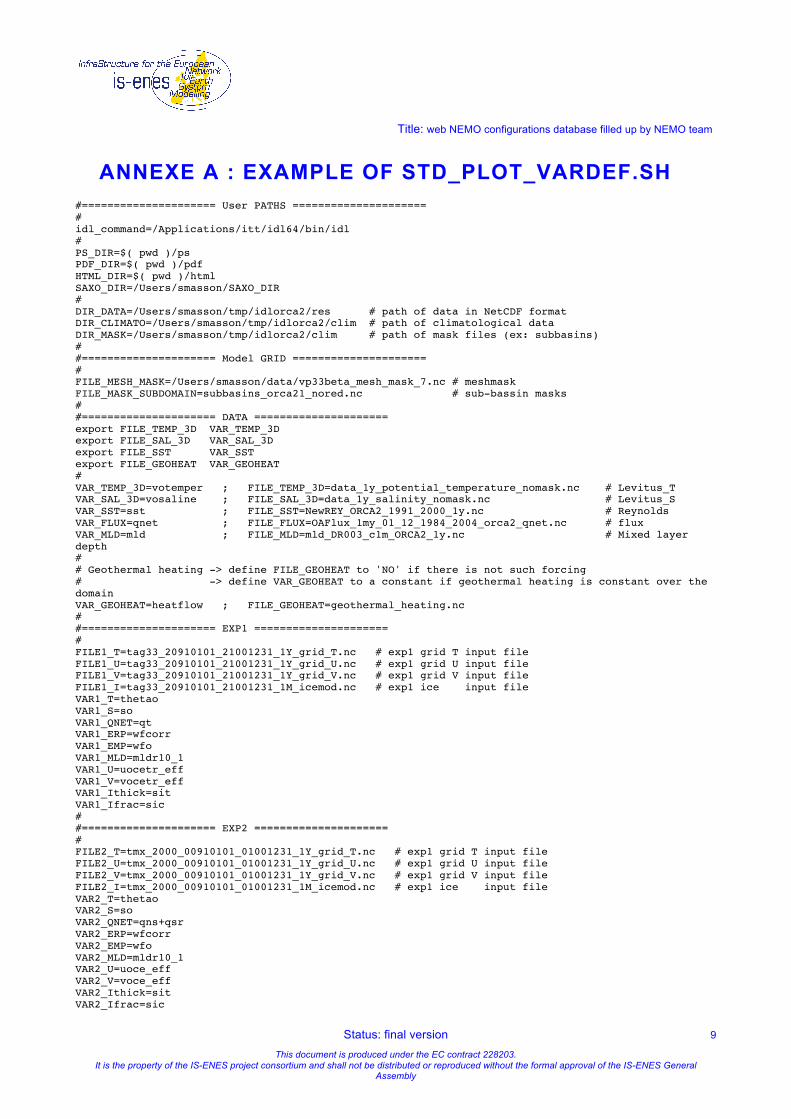
A special care has been taken to make the use of this tool as easy as possible and as flexible as possible. Each diagnostic is coded in a separated file to facilitate the evolution of the diagnostic tool. The use of IDL is transparent to the user. The user controls the description of the files on which the diagnostics will be applied through a simple ASCII file without any coding. 4 examples are provided with the source code. Annexe A and B of this document give an example of these ASCII files for spatially-averaged (std_ts_vardef.sh) and time-averaged (std_plot_vardef.sh) diagnostics. The execution of the diagnostics is done through a simple call to the shell script std_main.sh (provided with the sources):

> ./std_main.sh -plots # for the Time-averaged diagnostics > ./std_main.sh -ts # for the Spatially-averaged diag. > ./std_main.sh -help # to get help

By default, this shell script produces postscript files. However, it can also produce pdf or html files with the use of –pdf or –html options of std_main.sh:

> ./std_main.sh –plots -pdf > ./std_main.sh –ts -pdf > ./std_main.sh –plots -html > ./std_main.sh –ts -html

A description of the use of this tool is detailed in the README file provided with the source code.




4 . A F I R S T S E T O F E X A M P L E S We provide a first set of examples to illustrate the realisation of simulations following the protocol described in section 2 and the production of the associated diagnostics. This example is based on a set of simulations were performed with NEMO v3.2 that was the reference version when these experiments were performed. We also used libIGCM 1.4 as running scrip environment to facilitate the production of these simulations. These code versions were the reference versions when experiments were performed.

- NEMOv3.2 source code is available here: https://forge.ipsl.jussieu.fr/nemo/browser/tags/nemo_v3_2.

- libIGCM 1.4 source code is available here: https://forge.ipsl.jussieu.fr/libigcm/browser/tags/libIGCM_v1_4.

Users interested by the use of libIGCM with NEMOv3.2 can refer to the following web page: https://forge.ipsl.jussieu.fr/nemo/wiki/libIGCM An updated manual for NEMO v3.3 is available here: https://forge.ipsl.jussieu.fr/nemo/wiki/libIGCM_nemo_v_3_3 The following web page details all the procedure to perform these simulations: https://forge.ipsl.jussieu.fr/nemo/wiki/core2_cmip This page gives the “step by step” instructions to perform these simulations and lists the complete set of parameters (namelists, cpp keys…) that has been used to define the model configuration of these reference experiments. All simulations outputs are freely available on the following DODS server:

- http://dodsp.idris.fr/reee605/REFERENCE_CLIMATO/ - http://dodsp.idris.fr/reee605/REFERENCE_INTERAN/

Several examples of the plots and time series produced by this tool can be found at the following web page

• https://forge.ipsl.jussieu.fr/nemo/wiki/core2_cmip • http://www.nemo-ocean.eu/Using-NEMO/Configurations/ORCA2_LIM

As an illustration, there are 2 specific cases of plots and time series available respectively at http://dodsp.idris.fr/reee605/plots_CORE2/INTERAN/plots_pdf/tmx_int3.pdf and http://dodsp.idris.fr/reee605/ts_CORE2/INTERAN/ts_tmxint3_tmxint3.pdf .




BIBLIOGRAPHY Griffies, S M, A Biastoch, C Böning, F Bryan, G Danabasoglu, E P Chassignet, M H England, R Gerdes, H Haak, and R W Hallberg. 2009. Coordinated ocean-ice reference experiments (cores). Ocean Modelling 26 (1-2): 1-46. Large, W and S Yeager. 2009. The global climatology of an interannually varying air–sea flux data set. Climate Dynamics 33 (2): 341-364. http://dx.doi.org/10.1007/s00382-008-0441-3.




ANNEXE A : EXAMPLE OF STD_PLOT_VARDEF.SH #===================== User PATHS ===================== # idl_command=/Applications/itt/idl64/bin/idl # PS_DIR=$( pwd )/ps PDF_DIR=$( pwd )/pdf HTML_DIR=$( pwd )/html SAXO_DIR=/Users/smasson/SAXO_DIR # DIR_DATA=/Users/smasson/tmp/idlorca2/res # path of data in NetCDF format DIR_CLIMATO=/Users/smasson/tmp/idlorca2/clim # path of climatological data DIR_MASK=/Users/smasson/tmp/idlorca2/clim # path of mask files (ex: subbasins) # #===================== Model GRID ===================== # FILE_MESH_MASK=/Users/smasson/data/vp33beta_mesh_mask_7.nc # meshmask FILE_MASK_SUBDOMAIN=subbasins_orca21_nored.nc # sub-bassin masks # #===================== DATA ===================== export FILE_TEMP_3D VAR_TEMP_3D export FILE_SAL_3D VAR_SAL_3D export FILE_SST VAR_SST export FILE_GEOHEAT VAR_GEOHEAT # VAR_TEMP_3D=votemper ; FILE_TEMP_3D=data_1y_potential_temperature_nomask.nc # Levitus_T VAR_SAL_3D=vosaline ; FILE_SAL_3D=data_1y_salinity_nomask.nc # Levitus_S VAR_SST=sst ; FILE_SST=NewREY_ORCA2_1991_2000_1y.nc # Reynolds VAR_FLUX=qnet ; FILE_FLUX=OAFlux_1my_01_12_1984_2004_orca2_qnet.nc # flux VAR_MLD=mld ; FILE_MLD=mld_DR003_c1m_ORCA2_1y.nc # Mixed layer depth # # Geothermal heating -> define FILE_GEOHEAT to 'NO' if there is not such forcing # -> define VAR_GEOHEAT to a constant if geothermal heating is constant over the domain VAR_GEOHEAT=heatflow ; FILE_GEOHEAT=geothermal_heating.nc # #===================== EXP1 ===================== # FILE1_T=tag33_20910101_21001231_1Y_grid_T.nc # exp1 grid T input file FILE1_U=tag33_20910101_21001231_1Y_grid_U.nc # exp1 grid U input file FILE1_V=tag33_20910101_21001231_1Y_grid_V.nc # exp1 grid V input file FILE1_I=tag33_20910101_21001231_1M_icemod.nc # exp1 ice input file VAR1_T=thetao VAR1_S=so VAR1_QNET=qt VAR1_ERP=wfcorr VAR1_EMP=wfo VAR1_MLD=mldr10_1 VAR1_U=uocetr_eff VAR1_V=vocetr_eff VAR1_Ithick=sit VAR1_Ifrac=sic # #===================== EXP2 ===================== # FILE2_T=tmx_2000_00910101_01001231_1Y_grid_T.nc # exp1 grid T input file FILE2_U=tmx_2000_00910101_01001231_1Y_grid_U.nc # exp1 grid U input file FILE2_V=tmx_2000_00910101_01001231_1Y_grid_V.nc # exp1 grid V input file FILE2_I=tmx_2000_00910101_01001231_1M_icemod.nc # exp1 ice input file VAR2_T=thetao VAR2_S=so VAR2_QNET=qns+qsr VAR2_ERP=wfcorr VAR2_EMP=wfo VAR2_MLD=mldr10_1 VAR2_U=uoce_eff VAR2_V=voce_eff VAR2_Ithick=sit VAR2_Ifrac=sic




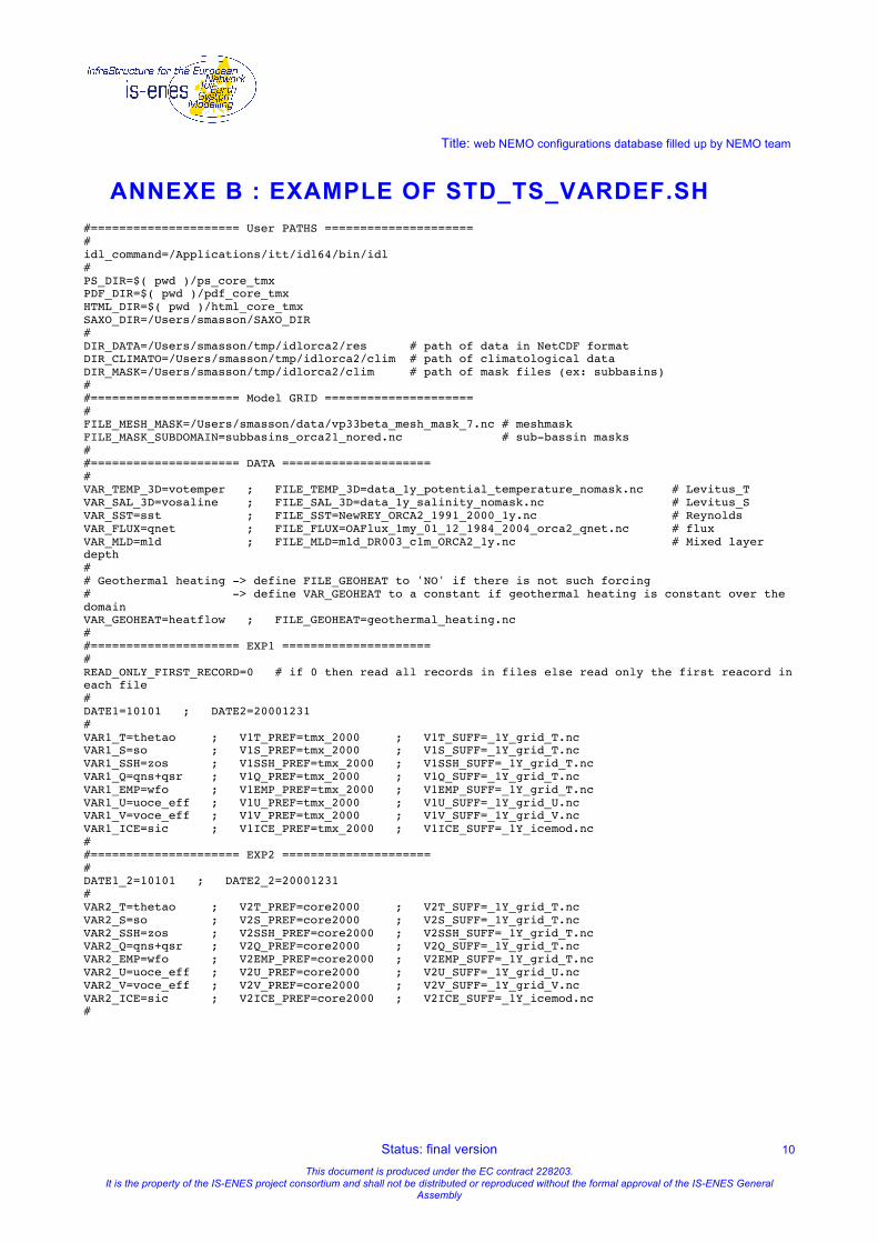
ANNEXE B : EXAMPLE OF STD_TS_VARDEF.SH #===================== User PATHS ===================== # idl_command=/Applications/itt/idl64/bin/idl # PS_DIR=$( pwd )/ps_core_tmx PDF_DIR=$( pwd )/pdf_core_tmx HTML_DIR=$( pwd )/html_core_tmx SAXO_DIR=/Users/smasson/SAXO_DIR # DIR_DATA=/Users/smasson/tmp/idlorca2/res # path of data in NetCDF format DIR_CLIMATO=/Users/smasson/tmp/idlorca2/clim # path of climatological data DIR_MASK=/Users/smasson/tmp/idlorca2/clim # path of mask files (ex: subbasins) # #===================== Model GRID ===================== # FILE_MESH_MASK=/Users/smasson/data/vp33beta_mesh_mask_7.nc # meshmask FILE_MASK_SUBDOMAIN=subbasins_orca21_nored.nc # sub-bassin masks # #===================== DATA ===================== # VAR_TEMP_3D=votemper ; FILE_TEMP_3D=data_1y_potential_temperature_nomask.nc # Levitus_T VAR_SAL_3D=vosaline ; FILE_SAL_3D=data_1y_salinity_nomask.nc # Levitus_S VAR_SST=sst ; FILE_SST=NewREY_ORCA2_1991_2000_1y.nc # Reynolds VAR_FLUX=qnet ; FILE_FLUX=OAFlux_1my_01_12_1984_2004_orca2_qnet.nc # flux VAR_MLD=mld ; FILE_MLD=mld_DR003_c1m_ORCA2_1y.nc # Mixed layer depth # # Geothermal heating -> define FILE_GEOHEAT to 'NO' if there is not such forcing # -> define VAR_GEOHEAT to a constant if geothermal heating is constant over the domain VAR_GEOHEAT=heatflow ; FILE_GEOHEAT=geothermal_heating.nc # #===================== EXP1 ===================== # READ_ONLY_FIRST_RECORD=0 # if 0 then read all records in files else read only the first reacord in each file # DATE1=10101 ; DATE2=20001231 # VAR1_T=thetao ; V1T_PREF=tmx_2000 ; V1T_SUFF=_1Y_grid_T.nc VAR1_S=so ; V1S_PREF=tmx_2000 ; V1S_SUFF=_1Y_grid_T.nc VAR1_SSH=zos ; V1SSH_PREF=tmx_2000 ; V1SSH_SUFF=_1Y_grid_T.nc VAR1_Q=qns+qsr ; V1Q_PREF=tmx_2000 ; V1Q_SUFF=_1Y_grid_T.nc VAR1_EMP=wfo ; V1EMP_PREF=tmx_2000 ; V1EMP_SUFF=_1Y_grid_T.nc VAR1_U=uoce_eff ; V1U_PREF=tmx_2000 ; V1U_SUFF=_1Y_grid_U.nc VAR1_V=voce_eff ; V1V_PREF=tmx_2000 ; V1V_SUFF=_1Y_grid_V.nc VAR1_ICE=sic ; V1ICE_PREF=tmx_2000 ; V1ICE_SUFF=_1Y_icemod.nc # #===================== EXP2 ===================== # DATE1_2=10101 ; DATE2_2=20001231 # VAR2_T=thetao ; V2T_PREF=core2000 ; V2T_SUFF=_1Y_grid_T.nc VAR2_S=so ; V2S_PREF=core2000 ; V2S_SUFF=_1Y_grid_T.nc VAR2_SSH=zos ; V2SSH_PREF=core2000 ; V2SSH_SUFF=_1Y_grid_T.nc VAR2_Q=qns+qsr ; V2Q_PREF=core2000 ; V2Q_SUFF=_1Y_grid_T.nc VAR2_EMP=wfo ; V2EMP_PREF=core2000 ; V2EMP_SUFF=_1Y_grid_T.nc VAR2_U=uoce_eff ; V2U_PREF=core2000 ; V2U_SUFF=_1Y_grid_U.nc VAR2_V=voce_eff ; V2V_PREF=core2000 ; V2V_SUFF=_1Y_grid_V.nc VAR2_ICE=sic ; V2ICE_PREF=core2000 ; V2ICE_SUFF=_1Y_icemod.nc #

web NEMO configurations database filled up by NEMO team

Documents

Transcript of web NEMO configurations database filled up by NEMO team