GeoinformaticaDOI 10.1007/s10707-008-0055-2

Web data retrieval: solving spatial range queriesusing k-nearest neighbor searches

Wan D. Bae · Shayma Alkobaisi · Seon Ho Kim ·Sada Narayanappa · Cyrus Shahabi

Received: 24 October 2007 / Revised: 25 July 2008 /Accepted: 28 August 2008© Springer Science + Business Media, LLC 2008

Abstract As Geographic Information Systems (GIS) technologies have evolved,more and more GIS applications and geospatial data are available on the web. Spatialobjects in a given query range can be retrieved using spatial range query − one of themost widely used query types in GIS and spatial databases. However, it can be chal-lenging to retrieve these data from various web applications where access to the data

The author’s work is supported in part by the National Science Foundation under awardnumbers IIS-0324955 (ITR), EEC-9529152 (IMSC ERC) and IIS-0238560 (PECASE) and inpart by unrestricted cash gifts from Microsoft and Google. Any opinions, findings, andconclusions or recommendations expressed in this material are those of the authors and do notnecessarily reflect the views of the National Science Foundation.

W. D. Bae (B)Department of Mathematics, Statistics and Computer Science,University of Wisconsin-Stout, Menomonie, WI, USAe-mail: baew@uwstout.edu

S. AlkobaisiCollege of Information Technology, United Arab Emirates University,Al-Ain, United Arab Emiratese-mail: shayma.alkobaisi@uaeu.ac.ae

S. H. KimDepartment of Computer Science Information & Technology,University of District of Columbia, Washington, DC, USAe-mail: skim@udc.edu

S. NarayanappaDepartment of Computer Science, University of Denver, Denver, CO, USAe-mail: snarayan@cs.du.edu

C. ShahabiDepartment of Computer Science, University of Southern California, Los Angeles, CA, USAe-mail: shahabi@usc.edu

Geoinformatica

is only possible through restrictive web interfaces that support certain types of que-ries. A typical scenario is the existence of numerous business web sites that providetheir branch locations through a limited “nearest location” web interface. For exam-ple, a chain restaurant’s web site such as McDonalds can be queried to find some ofthe closest locations of its branches to the user’s home address. However, eventhough the site has the location data of all restaurants in, for example, the state ofCalifornia, it is difficult to retrieve the entire data set efficiently due to its restrictiveweb interface. Considering that k-Nearest Neighbor (k-NN) search is one of the mostpopular web interfaces in accessing spatial data on the web, this paper investigatesthe problem of retrieving geospatial data from the web for a given spatial range queryusing only k-NN searches. Based on the classification of k-NN interfaces on the web,we propose a set of range query algorithms to completely cover the rectangular shapeof the query range (completeness) while minimizing the number of k-NN searches aspossible (efficiency). We evaluated the efficiency of the proposed algorithms throughstatistical analysis and empirical experiments using both synthetic and real data sets.

Keywords Range queries · k-Nearest neighbor queries · Web data · Web interfaces ·Web integration · GIS

1 Introduction

Due to the recent advances in Geographic Information Systems (GIS) technologiesand emergence of diverse web applications, a large amount of geospatial datahas become available on the web. For example, numerous businesses release thelocations of their branches on the web. The web sites of government organizationssuch as the US Postal Office provide the list of its offices close to one’s residence.Various non-profit organizations also publicly post a large amount of geospatial datafor different purposes.

There is a growing number of GIS applications that crawl or wrap various websources into one integrated solution for their users, such as Information Mediators.As an example, a fast food restaurant may need to know the distribution of otherrestaurants, e.g., McDonalds, in a certain geographic region for its future businessplan. There could be a government or environmental research organization needingto know about the characteristic of some businesses, social activities or changesin the nature. These applications, however, have difficulties to efficiently retrieveinformation for a certain region from various web sources because of their restrictiveweb interfaces [4]. On the web, access to geospatial data is only possible throughthe interfaces provided by the applications. These interfaces are usually designedfor one specific query type and hence cannot support general access to the data.They could retrieve data only using some particular types of queries such as k-NNquery. For example, the McDonalds web site provides a restaurant locator servicethrough which one can ask for the five closest restaurants from a given location.This type of web interface to search for a number of “nearest neighbors” from agiven geographical point (e.g., a mailing address) or an area (e.g., a zip code) is verypopular for accessing geospatial data on the web. It nicely serves the intended goalof quick and convenient dissemination of business location information to potentialcustomers. However, if the consumer of the data is a computer program, as in the case

Geoinformatica

of web data integration utilities (e.g., wrappers) and search programs (e.g., crawlers),such an interface may be a very inefficient way of retrieving all data in a given queryregion. To illustrate, suppose a web crawler wants to access the McDonalds web siteto retrieve all the restaurants in the state of California. Even though the site hasthe required information, the interface only allows the retrieval of five locations at atime. Even worse, the interface needs the center of the search as input. Hence, thecrawler needs to identify a set of nearest location searches that both covers the entirestate of California (for completeness) and has minimum overlap between the resultsets (for efficiency). The number of results returned even varies depending on theapplication. This problem necessitates for methods that utilize certain query types toprovide solutions to non-supported queries.

In this paper, we conceptualize the aforementioned problem into a more generalproblem of supporting spatial range query to retrieve web data in a given rectangularshaped region using k-Nearest Neighbor (k-NN) search. Besides web data integra-tion and search applications, the solution to this more general problem is beneficialfor other application domains in the areas of sensor networks, online maps and ad-hoc mobile networks where their applications require great deal of data integrationfor data analysis and decision support queries.

Figure 1 illustrates the challenges of this general problem through an example.Suppose that we want to find the locations of all the points in a given region(rectangle), and the only available interface is the k-NN search with a fixed k (k = 3in the example of Fig. 1). The only parameter that we can vary is the query pointfor the k-NN search (shown as cross marks in Fig. 1). Given a query point q, theresult of the k-NN search is a set of k nearest points to q. It defines a circle centeredat q with the radius equal to the distance from q to its kth nearest neighbor (i.e.,the 3rd closest point in this example). The area of this circle, covering part of therectangle, determines the searched (i.e., covered) portion of the rectangular region.To complete the range query, we need to identify a set of input locations of qcorresponding to a series of k-NN searches that would result in a set of circlescovering the entire rectangle.

Based on the classification of k-NN interfaces on the web, we propose a setof range query algorithms: the Density-Based (DB) algorithm for the case withknown statistics of the data sets assuming the most flexible k-NN interface (i.e., k

Fig. 1 A range query onthe web data

Pll

P ur

Range Query R

3-NN Searchq

Geoinformatica

is a user input), the Quad Drill Down (QDD) and Dynamic Constrained DelaunayTriangulation (DCDT) algorithms for the case with no knowledge of the distributionof the data sets and with the most restrictive k-NN interface (i.e., no control on thevalue of k), and the Hybrid (HB) of the two approaches, DB and QDD, for thesolution of the case with bounded values of k. Our algorithms guarantee the completecoverage of any given spatial query range. The efficiencies of the algorithms aremeasured by statistical analysis and empirical experiments using both synthetic andreal data sets.

The remainder of this paper is organized as follows: The problem is formallydefined in Section 2 and the related work is discussed in Section 3. In Section 4we propose our algorithms to solve range queries using a number of k-NN queries.Section 5 provides the performance evaluation of the proposed algorithms. We firstdiscuss the statistical analysis of DB and QDD. Then we present the efficiency of ouralgorithms through empirical experiments. Finally, Section 6 concludes the paper.

2 Problem definition

A range query in spatial database applications can be formally defined as follows:Let R be a given rectangular query region represented by two points, Pll and Pur,where Pll = (x1, y1) and Pur = (x2, y2). Pll and Pur refer to the lower-left corner andthe upper-right corner of R, respectively. Given a set of objects S and a region R,spatial range query finds all objects of S in R [8].

Similarly, a nearest neighbor (NN) query can be defined. Given a set of objects Sand a query point q, an NN query searches for a point p ∈ S such that dist(q, p) ≤dist(q, r) for any r ∈ S. The point p is the nearest neighbor of q. One can be interestedin finding more than one point, say k points, which are the nearest neighbors of thequery point q. This is called the k-Nearest Neighbor (k-NN) problem also knownas the top-k selection query. Given a set of objects S (with cardinality(S) = N),a number k ≤ N and a query point q, a k-NN query searches for a subset S′ ⊆ Swith cardinality(S′) = k such that for any p ∈ S′ and r ∈ S − S′, then distance(q, p) ≤distance(q, r) [16].

Our problem is defined as follows: Given a rectangular shaped query regionR, find all spatial objects within the query range using k-NN search interface assupported by various web applications. The complexity of this problem is unknown.Therefore only approximation results are provided. In reality, there can be morethan one web site involved in the given range query. Then, the general problem isto find all objects within the query region R using k-NN searches on each of theseweb sources and to integrate the results from the sources into one final query result.Figure 2a and b show examples of two different k-NN interfaces, k = 3 in (a) andk = 6 in (b). Two different data sets in the given same query region can be retrievedfrom the different web sources.

The optimization objective of this problem is to minimize the number of k-NNsearches while retrieving all objects in a given query region. Each k-NN search resultsin communication overhead between the client and the server in addition to theactual execution cost of the k-NN search at the server. The range query executionis broken down into four basic steps: 1) Client sends a request to the web server withthe query point q, 2) Server executes the k-NN search using q, 3) Server returns the

Geoinformatica

q

Westminster

Northglenn

Thornton

Lakewood

Aurora

Parker

Centennial

Littleton

Highlands Ranch

Golden

Cherry Hills village

Englewood

Wheat Ridge

Indian Hills

Denver

Glendale

Arvada

Broomfield

285

I 25

I 225

I 70

ARVADAARVADACOUNTYCOUNTY

285 2852855

Westminster

Northglenn

Thornton

Lakewood

Aurora

Parker

Centennial

Littleton

Highlands Ranch

Golden

Cherry Hills village

Englewood

Wheat Ridge

Indian Hills

Denver

Glendale

Arvada

Broomfield

285

I 25

I 225

I 70

ARVADAARVADACOUNTYCOUNTY

H

H

HHH

H HH

H

H H

H

H

H

(a) A range query using 3-NN search (b) A range query using 6-NN search

Fig. 2 Range queries on the web data (a, b)

result of the k-NN search to client, 4) Client prunes the result (client may invokeadditional requests to server). Let Cn be the total cost of the range query and Cq,Cknn, Cres, and Cpru represent the cost associated with each of the four steps, where nis the total number of k-NN searches required to complete a range query. Then, Cn

is defined as follows:

Cn = Cpru(n) +n∑

i=1

[Cq(i) + Cknn(i) + Cres(i)].

Steps 1 and 3 both involve communication over the network. For step 2, we assumethat any of the known k-NN search algorithms [6, 7, 13, 17] is available to the webapplications; if any tree index structure is used, the complexity of k-NN search isknown to be O(logN + k) [7], where N is the total number of objects in the database,and k is the number of objects we want to retrieve. The cost of step 4 is the CPU timerequired to prune the k-NN result at the client side. If additional k-NN searches arerequired to cover the query region, then additional costs of all Cq, Cknn, and Cres mustbe taken into account. However, Cpru is required only once for a given query. Hence,we focus on reducing the number of k-NN searches in this paper while placing ourcircles to have as few overlaps as possible. Finally, the fact that we do not know theradius of each circle prior to the actual evaluation of its corresponding k-NN querymakes the problem even harder.

To summarize, the optimal solution should find a minimal set of query locationsthat minimizes the number of k-NN searches to completely cover the given queryregion. In many web applications, the client has no knowledge about the data set atthe server and no control over the value of k (i.e., k is fixed depending on the webapplications). These applications return a fixed number of k nearest objects to theuser’s query point. A typical value of k in real applications rages from 5 to 20 [4],multiple queries are evaluated to completely cover a reasonably large region.

In this paper we consider all possible k-NN interfaces. Any web applicationssupporting k-NN search can be classified based on the value of k:

1. The value of k is fixed, and the user does not have any control over k−the generalproblem. Many applications always return a fixed number of k nearest objects tothe user’s query point. Different applications may have different values of k.

Geoinformatica

2. The value of k can be any positive integer determined by users. Some webapplications accept user-defined k values for their k-NN searches.

3. The value of k can be any positive integer less than or equal to a certain value.Some web applications support k-NN search with user-defined k values but allowonly a bounded range of k values.

To simplify the discussion, we made the following assumptions: 1) a range querywill be supported by a single web source; 2) a web application supports only one typeof k-NN query (fixed, flexible or bounded k value); 3) a k-NN search takes a querypoint q as an input parameter.

3 Related work

Some studies have discussed the problems of data integration and query processingon the web [12, 22]. A survey of the general problems in the integration of web datasources can be found in [9]. The paper discussed challenges of the heterogeneousnature of the web and different ways of describing the same data, and proposedgeneral ideas of how to tackle those problems. Nie et al. [12] presented a queryprocessing framework for web-based data integration and implemented the evalua-tion of query planning and statistics gathering modules. The problem of querying websites through limited query interfaces has been studied in the context of informationmediation systems in [22]. Based on the capabilities of the mediator, the authorsproposed an idea to compute the set of supported queries.

Several studies have focused on performing spatial queries on the web [1, 4, 10].In [1], the authors demonstrated an information integration application that allowsusers to retrieve information about theaters and restaurants from various U.S. cities,including an interactive map. Their system showed how to build applications rapidlyfrom existing web data sources and integration tools. The problem of spatial coverageusing only the k-NN interface was introduced in [4]. The paper provided a quad-treebased approach. A quad-tree data structure was used to check the complete coverageby marking regions that have been covered so far. The authors follow a greedyapproach using the coverage information to determine the next query’s position. Ourprevious work [2] provided an efficient and complete solution for the problem in thecase when the value of k is fixed and users have no control on the web interfaceand no knowledge on the data. This paper extends our previous work and providescomprehensive solutions on the most general case based on the classification of allpossible k-NN interfaces on the web. In our proposed QDD algorithm, we followa systematic way of dividing the region to be covered which spare us the need ofthe quad tree data structure used in [4]. This systematic division of the range queryprovides the information of coverage without needing to access any data structure todecide on the next query’s position.

The problem of supporting k-NN query using range queries was studied in [10].The idea of successively increasing query range to find k points was describedassuming statistical knowledge of the data set. This is the complement to the problemwe are focusing on.

Many k-NN query algorithms have been proposed [6, 13, 17]. In [13], the authorsproposed branch-and-bound R-tree traversal algorithm to find the k nearest neigh-bors of a given query point. They also introduced two metrics for both searching

Geoinformatica

and pruning, which are MINDIST that produces the most optimistic ordering andMINMAXDIST that produces the most pessimistic ordering possible. A new costmodel for optimizing nearest neighbor searches in low and medium dimensionalspaces was proposed in [17]. They proposed a new method that captures theperformance of nearest neighbor queries based on approximation. Their techniquewas based on the vicinity rectangles and the Minkowski rectangles. In [6], given aset of points, the authors proposed two algorithms to solve two k nearest neighborrelated problems. The first enumerates the k smallest distances between pairs ofpoints in nondecreasing order and the second finds the k nearest neighbors of eachpoint. Both are based on a Delaunay triangulation.

The Delaunay triangulation and Voronoi diagram based approaches have beenstudied for various purposes in wireless sensor networks [15, 19, 21]. In [19], theauthors used the Vornonoi diagram to discover the existence of coverage holes,assuming that each sensor knows the location of its neighbors. The region is parti-tioned into Voronoi cells and each cell contains one sensor. If a cell is not coveredby a sensor, the coverage holes are found. The authors use a greedy approach bytargeting the largest hole which is a Voronoi cell as the next region to be covered.Sensors replacement that have fixe coverage radius by minimizing the movementsof the sensors is one of the main ideas in their paper. Similarly, our proposedDCDT algorithm greedily targets the largest uncovered region, a triangle, to becovered, however, coverage is determined by the non fixed radius of the k-NNquery. The Delaunay triangulation and Vornonoi diagram was used to determine themaximal breach path (MBP) and the maximal support path (MSP) for a given sensornetwork in [11]. In [21] proposed a wireless sensor network deployment method wasproposed based on the Delaunay triangulation. This method was applied for planningthe positions of sensors in an environment with obstacles. Their main goal was tomaximize the coverage of the sensors and not to cover the complete region. Eachcandidate position of a sensor is generated from the current sensor configurationby calculating its scored using a probabilistic sensor detection model. The proposedapproach retrieved the location information of obstacles and pre-deployed sensors,then constructed a Delaunay triangulation to find candidate positions of new sensors.In our DCDT algorithm, a constrained Delaunay triangulation (CDT) is used to finduncovered region with the most coverage gains. The CDT is dynamically updatedwhile covering the query region with k-NN circles.

4 Range query algorithms using k-NN search

We study and investigate different approaches for all possible k-NN search interfacesdefined in Section 2. We develop four spatial range query algorithms that utilizek-NN search to retrieve all objects in a given rectangular shaped query region:Density Based (DB) for flexible values of k, Quad Drill Down (QDD) and DynamicConstrained Delaunay Triangulation (DCDT) for fixed values of k, and Hybrid(HB) for bounded values of k.

The notations in Table 1 are used throughout this paper and Fig. 3 illustrates anexample of range query using 5-NN search using the notations. Let R be a givenquery region and CRq be the circle inscribing R having q and Rq as the center andradius of CRq , respectively. Notice that q is also the center point of R. Let Pk =

Geoinformatica

Table 1 Notations

Notation Description

R A query region (rectangle)Pll The lower-left corner point of RPur The upper-right corner point of Rq The query point for a k-NN searchRq Half of the diagonal of R; the distance from q to Pll

CRq Circle inscribing R; the circle of radius Rq centered at qPk The set of k nearest neighbors obtained by a k-NN search ordered ascendingly

by distance from q, i.e., P5 = {p1, p2, p3, p4, p5} in Fig. 3r The distance from q to the farthest point pk in Pk

Cr k-NN circle; the circle of radius r centered at qC

′r Tighter bound k-NN circle; the circle of radius ε · r centered at q

{p1, p2, ..., pk} be the k nearest neighbors, ordered by distance from q obtained bythe k-NN search with q as the query point. Let qpk = r, i.e., r is the distance from qto the farthest point pk. Let Cr be the circle of radius r centered at q, which we referto as a k-NN circle.

If r > Rq, then the k-NN search must return all the points inside CRq . Therefor, wecan obtain all the points inside the region R after pruning out any points of Pk thatare outside R but inside Cr. Then, the range query is complete. Otherwise, we needto perform some additional k-NN searches to completely cover R. For example, ifwe use a 5-NN search for the data set shown in Fig. 3, then the resulting Cr is smallerthan CRq . Note that it is not sufficient to have r ≥ Rq in order to retrieve all thepoints inside R when q has more than one kth nearest neighbor since one of them willbe randomly returned as q’s kth nearest neighbor. Assuming four points in the fourcorners of R, four points strictly inside of Cr, and the value of k = 5, the returnedresult is P5 = {p1, p2, ..., p5}. The condition, r > Rq, is required since 5-NN searchrandomly picks one from four points on the corners as p5 discarding the rest of threepoints. As a result, we use r > Rq as a terminating condition in our algorithms.

Fig. 3 A range query using5-NN search

C r

C

Range Query R

Rq

r

P

P

ll

ur

q

Rq

P1

P5

P3

P2

P4

Geoinformatica

4.1 Algorithm using flexible values of k

Some web applications can support k-NN interface with flexible values of k so thatusers can choose any integer value for k-NN search. Some also provide the totalnumber of data (objects, i.e., stores or branches) and their service area. By carefullydetermining the k value, a range query can be evaluated with a single k-NN search ifall the objects in the given query region can be found from the results of the very firstk-NN search. Based on this assumption, we propose the Density Based (DB) rangequery algorithm, a statistical approach for retrieving web data in a given region.

The main idea of DB is to find a good approximation of the k value using somestatistical knowledge of the web data, i.e., the density of the data sets. Assuming thatthe density information of web data is available, let N be the total number of objectsin a web source and Aglobal be the area of the minimum bounding rectangle (MBR)that includes all those objects. Then, two estimation methods are considered: globaland local estimations.

The global estimation method is as follows: The global density is NAglobal

, and Rq ishalf the diagonal of R as described in Fig. 3. We then estimate the number of objects(k) that are inside CRq with the parameters, Aglobal , N, and Rq:

k = π R2q · N/Aglobal. (1)

k is used to call the first k-NN search to the Web data. From the k-NN result, Cr (k-NN circle) is expected to match CRq . If Cr ≤ CRq , then we need extra k-NN searches.Thus, we need to re-estimate the k value using the local estimation.

The local estimation method is as follows: Let Alocal be the area of the currentCr, Area(Cr)=πr2 and k be the value used by the previous k-NN search. The localdensity is k

Alocal. Then the new estimation of k is:

k′ = π R2q · k/Alocal. (2)

k′ is used to call the next k-NN search to the Web data.In the DB algorithm we first estimate the initial k using the global density of the

data set. The center point of the query region R is the query point q (see Fig. 3).If Cr is not larger than CRq , the value of k is under-estimated because Cr cannotcover the entire R. Then, it is necessary to increase the k value. A new value k′ isthen calculated using the local density. This local estimation of k′ continues until Cr

becomes larger than CRq . If Cr is larger than CRq , the result of k-NN includes all theobjects inside CRq . Finally, pruning is required to eliminate the objects outside R butinside CRq .

Even though we determine the value of k by taking advantage of known statistics,there can be a significant number of underestimated/overesitmated cases due tostatistical variation. Underestimation of k value incurs an expensive cost, i.e., a newk-NN search requiring all new Cpru, Cq, Cknn, and Cres, while overestimation of kvalue does not.1 From the observation that a slight overestimation of k value canabsorb a significant amount of statistical variance (i.e., more range queries can beevaluated in a single k-NN search) and it does not create a significant overhead

1Actually, overestimation introduce a slight overhead in each cost function but it is way lower thanthe overhead caused by underestimation.

Geoinformatica

cost, we introduce the overestimation constant, ε, for a loosely bounded k value.To obtain a loosely bounded k value, the k value is multiplied by ε (ε > 1). Theε value can be determined from empirical experiments and statistics based uponthe density and distribution of the data set. Algorithm 1 describes the DB rangequery. The DB algorithm will be evaluated through both statistical analysis andempirical experiments in Section 5. We will also demonstrate how the ε value affectsthe performance of the DB algorithm.

Algorithm 1 DB rangeQuery(Pll, Pur, Aglobal , N)

1: ε ← a constant factor2: Pc.x ← (Pll.x + Pur.x)/23: Pc.y ← (Pll.y + Pur.y)/24: Rq ← √

(Pur.x − Pc.x)2 + (Pur.y − Pc.y)2

5: q ← Pc

6: kinit ← estKvalue(Rq, Aglobal , N) // using Eq. (1)7: Knn{} ← kNNSearch(q, ε · kinit)

8: r ← maxDistkNN(q, Knn{})9: k ← kinit

10: while r ≤ Rq do11: clear Knn{}12: Alocal ← π · r2

13: k ← estKvalue(Rq, Alocal , k) // using Eq. (2)14: Knn{} ← kNNSearch(q, ε · k)

15: r ← maxDistkNN(q, Knn{})16: end while17: result{} ← pruneResult(Knn{}, Pll, Pur)

18: return result{}

4.2 Algorithms using fixed values of k

In many web applications, the client has no knowledge of the data set at the serverand no control over the value of k (i.e., k is fixed). Considering a typical value of kin real applications, which ranges from 5 to 25 [4], in general, multiple queries arerequired to completely cover a reasonably large R.

Our approach to this general range query problem on the web is as follows: 1)divide the query region R into subregions, R = {R1, R2, ..., Rm}, such that any Ri ∈R can be covered by a single k-NN search, 2) obtain the resulting points from thek-NN search on each of the subregions, 3) combine the partial results to provide acomplete result to the original range query R. Then, the main focus is how to divideR so that the total number of k-NN searches can be minimized. We consider thefollowing three approaches:

1. A naive approach: divide the entire R into equi-sized subregions (grid cells) suchthat any cell can be covered by a single k-NN search.

2. A recursive approach: conduct a k-NN search in the current query region, dividethe current query region into subregions with same sizes if the k-NN search failsto cover R, and call k-NN search for each of these subregions. Repeat the processuntil all subregions are covered.

Geoinformatica

3. A greedy and incremental approach: divide R into subregions with differentsizes. Then select the largest subregion for the next k-NN search. Check thecovered region by the k-NN search and select the next largest subregion foranother k-NN search.

Taking the example in Fig. 3, if r > Rq, then the k-NN search must return allthe points inside CRq . Therefore, we can obtain all the points inside the region Rafter pruning out any points of Pk that are outside R but inside Cr. Then, the rangequery is complete. Otherwise, we need to perform some additional k-NN searchesto completely cover R. For example, if we use a 5-NN search for the data set shownin Fig. 3, then the resulting Cr is smaller than CRq . For the rest of this section, wefocus on the latter case, which is a more realistic scenario. In a naive approach,R is divided into a grid where the size of cells is small enough to be covered bya single k-NN search. However, it might not be feasible to find the exact cell sizewith no knowledge of the data sets. Even in the case that we obtain such a grid,this approach is inefficient due to large amounts of overlapping areas among k-NNcircles and wasted time to search empty cells considering that most real data setsare not uniformly distributed. Therefore, we provide a recursive approach and anincremental approach in the following subsections.

4.2.1 Quad drill down (QDD) algorithm

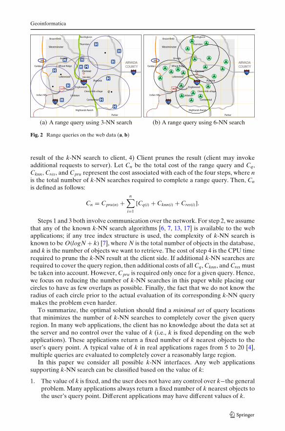
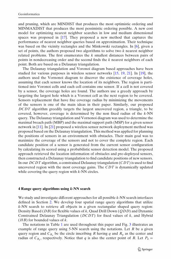
We propose a recursive approach, the Quad Drill Down (QDD) algorithm, as asolution to the range query problem on the web using the properties of the quad-tree. A quad-tree is a tree whose nodes either are leaves or have four children, and itis one of the most commonly used data structures in spatial databases [14]. The quad-tree represents a recursive quaternary decomposition of space wherein at each levela subregion is divided into four equal sized subregions (quadrants). The propertiesof the quad-tree provide a natural framework for optimizing decomposition [20].Hence, the quad-tree can give us an efficient way to divide the query region R. Weadopt the partitioning idea of the quad-tree, but we do not actually construct thetree. The main idea of QDD is to divide R into equal-sized quadrants, and thenrecursively divide quadrants further until each subregion is fully covered by a singlek-NN search so that all objects in it are obtained. An example of QDD is illustratedin Fig. 4 (when k = 3), where twenty one k-NN calls are required to retrieve all thepoints in R.

Algorithm 2 describes QDD. First, a k-NN search is invoked with a point q whichis the center of R. Next, the k-NN circle Cr is obtained from the k-NN result. If Cr

is larger than CRq , it entirely covers R, then all objects in R are retrieved. Finally,a pruning step is necessary to retrieve only the objects that are inside R − a trivialcase. However, if Cr is smaller than or equal to CRq , the query region is partitionedinto four subregions by equally dividing the width and height of the region by two.The previous steps are repeated for every new subregion. The algorithm recursivelypartitions the query region into subregions until each subregion is covered by a k-NNcircle. The pruning step eliminates those objects that are inside the k-NN circle butoutside the subregion. Statistical analysis of QDD is demonstrated in Section 5.2 aswell as the empirical experiment results.

Geoinformatica

Fig. 4 A Quad Drill Downrange query (a, b)

P ll

P ur

Range Query R

q3

x

xx

x x

x

x

x x

x

x

x

x x xx x

x

x x

q2

qx

q1 q4

3-NN Search

P3

P2 P1

P0

q

q1 q3 q4

q11 q12 q13 q14 q21 q22 q23 q24 q41 q42 q43 q44

q111 q112 q113 q114

(a) A QDD Range Query

(b) A Quad-tree representation of QDD

q2

4.2.2 Dynamic constrained delaunay triangulation (DCDT) Algorithm

We propose the Dynamic Constrained Delaunay Triangulation (DCDT) algorithmas another approach to solve the range query using the most restricted k-NNinterface − a greedy and incremental approach using the Constrained DelaunayTriangulation (CDT).2 DCDT uses triangulations to divide the query range andkeeps track of covered triangles by k-NN circles using the characteristics of con-strained edges in CDT. DCDT greedily selects the largest uncovered triangle forthe next k-NN search while QDD follows a pre-defined order.

To overcome redundant k-NN search on the same area, DCDT includes apropagation algorithm to cover the maximum possible area within a k-NN circle.Thus, no k-NN search will be wasted because a portion of a k-NN circle is alwaysadded to the covered area of the query range.

2The terms, CDT and DCDT, are used for both the corresponding triangulation algorithms and thedata structures that support these algorithms in this chapter.

Geoinformatica

Algorithm 2 QDDrangeQuery(Pll , Pur)1: q ← getCenterOfRegion(Pll , Pur)2: Rq ← getHalfDiagonal(q, Pll, Pur)3: Knn{} ← add kNNSearch(q)

4: r ← getDistToKthNN(q, Knn{})5: if r > Rq then6: result{} ← pruneResult(Knn{}, Pll, Pur)

7: else8: clear Knn{}9: P0 ← (q.x, Pll.y)

10: P1 ← (Pur.x, q.y)

11: P2 ← (Pll.x, q.y)

12: P3 ← (q.x, Pur.y)

13: Knn{} ← add QDDrangeQuery(Pll, q) // q114: Knn{} ← add QDDrangeQuery(P0, P1) // q415: Knn{} ← add QDDrangeQuery(P2, P3) // q216: Knn{} ← add QDDrangeQuery(q, Pur) // q317: result{} ← Knn{}18: end if19: return result{}

Data Structure for DCDT Given a planar graph G with a set of n vertices, P,in the plane, a set of edges, E, and a set of special edges, C, CDT of G is atriangulation of the vertices of G that includes C as part of the triangulation [5], i.e.,all edges in C appear as edges of the resulting triangulation. These edges are referredas to constrained edges, and they are not crossed (destroyed) by any other edgesof triangulation. CDT is also called as an obstacle triangulation or a generalizedDelaunay Triangulation. Figure 5 illustrates a graph G and the corresponding CDT.In this example, Fig. 5a shows a set of vertices, P = {P1, P2, P3, P4, P5, P6, P7}, anda set of constrained edges, C = {C1, C2}. Figure 5b shows the result of CDT thatincludes the constrained edges of C1 and C2 as part of the triangulation.

We define the following data structures to maintain the covered and uncoveredregions of R:

• pList: a set of all vertices of G; initially {Pll, Prl, Plr, Pur}• cEdges: a set of all constrained edges of G; initially empty• tList: a set of all uncovered triangles of G; initially empty

pList and cEdges are updated based on the current covered region by a k-NNsearch. R is then triangulated (partitioned into subregions) using CDT with thecurrent pList and cEdges. For every new triangulation, we obtain a new tList.DCDT keeps track of covered triangles (subregions) and uncovered triangles; cov-ered triangles are bounded by constrained edges (i.e., all three edges are constrainededges) and uncovered triangles are kept in tList, which are sorted in descendingorder by the area of the triangles. DCDT chooses the largest uncovered trianglein tList and calls k-NN search using the centroid, which always lies inside the triangleas opposed to the center of the triangle, as the query point. Our algorithm uses aheuristic approach that picks the largest triangle from the list of uncovered triangles.

Geoinformatica

Fig. 5 Example ofConstrained Delaunaytriangulation (a, b)

p2

p6

p7

p5

p4

p3

p1

c1

c2

p2

p6

p7

p5

p4

p3

p1 c

1

c2

(a) Constrained edges (b) CDT

The algorithm terminates when no more uncovered triangles exist. We describe thedetails of DCDT shown in Algorithm 3 and Algorithm 4 in the following sections.

The First k-NN search in DCDT DCDT invokes the first k-NN search using thecenter point of the query region R as the query point q. Figure 6a shows an exampleof a 3-NN search. If the resulting k-NN circle Cr completely covers R (r > Rq), thenwe prune and return the result − a trivial case. If Cr does not completely cover R,DCDT needs to use C

′r, which is a little smaller circle than Cr, for checking covered

regions from this point for further k-NN searches. We have previously discussed thepossibility that the query point q has more than one kth nearest neighbor, and one ofthem is randomly returned. In that case, DCDT may not be able to retrieve all thepoints in R if it uses Cr. Hence we define C

′r using r

′ = δ · r, where 0 < δ < 1 (δ = 0.99is used in our experiment).

DCDT creates an n-gon inscribed into C′r. Choosing the value of n depends on

the tradeoff between computation time and the coverage of area; n = 6 (a hexagon)is used in our experiments as shown in Fig. 6b. All vertices of the n-gon are addedinto pList. To mark the n-gon as a covered region, the n-gon is triangulated and theresulting edges are added as constrained edges into cEdges (getConstrainedEdges()line 12 of Algorithm 3). The algorithm constructs a new triangulation with the current

P ll

P ur

q

C r

P ll

P ur

q

C r ‘

(a) Query region R and center point q (b) Marking a hexagon as covered region

Fig. 6 An example of first k-NN call in query region R (a, b)

Geoinformatica

pList and cEdges, then a newly created tList is returned (constructDCDT() line 13of Algorithm 3).

Covering Regions DCDT selects the largest uncovered triangle from tList forthe next k-NN search. With the new C

′r, DCDT updates pList and cEdges and

creates a new triangulation. For example, if an edge lies within C′r, then DCDT adds

it into cEdges; on the other hand, if an edge intersects C′r, then the partially covered

edge is added into cEdges. Figure 7 shows an example of how to update and maintainpList, cEdges and tList. 1 (max) is the largest triangle in tList, therefore 1 isselected for the next k-NN search. DCDT uses the centroid of 1 as the querypoint q for the k-NN search. C

′r partially covers 1: vertices v5 and v6 are inside C

′r but

vertex v3 is outside C′r. C

′r intersects 1 at k1 along v3v6 and at k2 along v3v5, hence,

k1 and k2 are added into pList (getCoveredVertices() line 3 of Algorithm 4). LetRc be the covered area (polygon) of 1 by C

′r (Fig. 7c). Then Rc is triangulated

and the resulting edges, k1k2, k1v6, k2v5, v5v6 and k1v5 are added into cEdges.The updated pList and cEdges are used for constructing a new triangulation of R(Fig. 7c).

Algorithm 3 DCDTrangeQuery(Pll , Pur, δ)1: pList{} ← {Pll, Prl, Plr, Pur}; cEdges{} ← { }; tList{} ← { };2: Knn{} ← { } // all objects retrieved by k-NN search3: q ← getCenterOfRegion(Pll , Pur)4: Knn{} ← add kNNSearch(q)5: r ← getDistToKthNN(q, Knn{})6: Cr ← circle centered at q with radius r7: Rq ← getHalfDiagonal(q, Pll, Pur)8: if r ≤ Rq; Cr does not cover the given region R then9: C

′r ← circle centered at q with radius δ · r

10: Ng ← create an n-gon inscribing C′r with q as the center

11: pList{} ← add {all vertices of Ng}12: cEdges{} ← getConstrainedEdges({all vertices of Ng})13: tList{} ← constructDCDT(pList{}, cEdges{})14: while tList is not empty do15: mark all triangles in tList to unvisited16: max ← getMaxTriangle()17: q ← getCentroid(max)18: Knn{} ← add kNNSearch(q)19: r ← getDistToKthNN(q, Knn{})20: C

′r ← circle centered at q with radius δ · r

21: checkCoverRegion(max, C′r, pList{}, cEdges{})

22: tList{} ← constructDCDT(pList{}, cEdges{})23: end while24: end if25: result{} ← pruneResult(Knn{}, Pll, Pur)26: return result{}

Geoinformatica

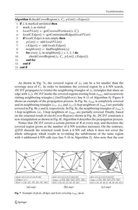
Algorithm 4 checkCoverRegion(, C′r, pList{}, cEdges{})

1: if is marked unvisited then2: mark as visited3: localPList{} ← getCoveredVertices(, C

′r)

4: localCEdges{} ← getConstrainedEdges(localPList)5: if localCEdges is not empty then6: pList{} ← add localPList{}7: cEdges{} ← add localcEdges{}8: neighbors{} ← findNeighbors()9: for every i in neighbors{}, i = 1, 2, 3 do

10: checkCoverRegion(i, C′r, pList{}, cEdges{})

11: end for12: end if13: end if

As shown in Fig. 7c, the covered region of 1 can be a lot smaller than thecoverage area of C

′r. In order to maximize the covered region by a k-NN search,

DCDT propagates to (visits) the neighboring triangles of 1 (triangles that share anedge with 1). DCDT marks the covered regions starting from max, and recursivelyvisiting neighboring triangles ( f indNeighbors() line 8–11 of Algorithm 4). Figure 8shows an example of the propagation process. In Fig. 8a, max is completely coveredand its neighboring triangles 11, 12 and 13 (1-hop neighbors of max) are partiallycovered in Fig. 8b, c and d, respectively. In Fig. 8e, the neighboring triangles of max’s1-hop neighbors, i.e., 2-hop neighbors of max, are partially covered. Finally, basedon the returned result of checkCoverRegion() shown in Fig. 8e, DCDT constructs anew triangulation as shown in Fig. 8f. Algorithm 4 describes the propagation process.

Notice that DCDT covers a certain portion of R at every step, and therefore thecovered region grows as the number of k-NN searches increases. On the contrary,QDD discards the returned result from a k-NN call when it does not cover thewhole subregion, which results in re-visiting the subdivisions of the same regionwith 4 additional k-NN calls (see line 5–16 in Algorithm 2). Also note that the cost

‘ ‘

pList ={v1,v2,v3,v4,v5,v6} cEdges ={ } tList = { 1Δ , 2Δ , 3Δ , 4Δ , 5Δ , 6Δ }

pList ={v1,v2,v3,v4,v5,v6,k1,k2}

cEdges ={ 65vv , 16kv , 21kk , 52vk , 15kv } tList = { 1Δ , 2Δ , 3Δ , 4Δ , 5Δ , 6Δ }

pList ={v1,v2,v3,v4,v5,v6,k1,k2}

cEdges ={ 65vv , 16kv , 21kk , 52vk , 15kv } tList = { 2Δ , 5Δ , 6Δ , 7Δ , 8Δ , 9Δ , 10Δ , 11Δ }

(a) step1 (b) step2 (c) step3

Fig. 7 Example of pList, cEdges and tList: covering max (a–c)

Geoinformatica

(a) (b) (c)

(d) (e) (f)

Fig. 8 Example of checkCoverRegion() (a–f)

of triangulation is negligible as compared to k-NN search because triangulation isperformed in memory and incrementally.

DCDT repeats the processes until no more uncovered regions exist. The resultedk-NN circle Cr can either completely cover R or partially cover R. The example inFig. 9a shows the first step of DCDT. The shaded triangles are covered-subregionsand all the edges of these triangles are now considered as constrained edges.Figure 9b and c illustrate examples of DCDT result after the 5th k-NN search andthe 9th k-NN search, respectively.

Cases of Covered Regions In this section we define the cases of covered region Rc

and discuss the details of Algorithm 4. Let Cr be the returned k-NN circle centeredby q and T be the given triangle that we consider covering using Cr. Let a, b and c

Pll Pll Pll

Cr

Cr

Cr

Pur Pur Pur

(a) 1st k-NN call (12%) (b) 5th k-NN call (52%) (c) 9th k-NN call (92%)

Fig. 9 Example of DCDT w/k=15 (coverage rate) (a–c)

Geoinformatica

Fig. 10 Examples of the casesfor covered region Rc (a–h)

(a) Case 1 (b) Case 2

(c) Case 3.1 (d) Case 3.2

(e) Case 4.1 (f) Case 4.2

(g) Case 4.3a (h) Case 4.3b

be the three vertices of T . The following cases are defined for covered region Rc,and the corresponding examples are illustrated in Fig. 10.

Case 1: All three vertices, a, b and c, are inside Cr so that T is completely coveredby a k-NN search: Rc is abc.

Case 2: Two vertices (say a and b) are inside Cr but the third vertex (say c)is outside Cr. Then Cr has one intersection (say b ′) with bc and oneintersection (say a′) with ca: Rc is the polygon with the edges, ab , aa′, bb ′and a′b ′.

Case 3: One vertex (say a) is inside Cr but two other vertices (say b and c) areoutside Cr;

Case 3.1: Cr has one intersection (say b ′) with ab and one intersection(say c′) with ca: Rc is ab ′c′ .

Geoinformatica

Case 3.2: Cr has one intersection (say b ′)with ab , one intersection (sayc′) with ca, and either one intersection (say k1) or two intersec-tions (say k1 and k2) with bc: Rc is the polygon with the edges,ab ′, b ′k1, k1k2, k2c′ and c′a.

Case 4: All three vertices are outside Cr;

Case 4.1: The center of Cr is inside T and Cr has either no intersectionor only one intersection with all edges of T : create an n-goninscribed into Cr and then Rc is n-gon.

Case 4.2: Cr has two intersections with at least two edges of T : Let theseintersection points be k1, k2,...,ki where 4 ≤ i ≤ 6. Rc is thepolygon with the edges, k1k2,k2k3,..., kik1.

Case 4.3: Cr has two intersections with one edge (say ab) of T . Let thesetwo intersections be k1 and k2 and let m be the center point ofk1k2:

Case 4.3a: If the center of Cr is inside T , then add k1k2,then create an n-gon inscribed into Cr and find theintersections of the n-gon and ab . Let S be a set ofpoints that includes: 1) the points of n-gon that areinside T , 2) the intersection points of the n-gonand ab , S = {k1, k2, ..., ki}. Rc is the polygon withedges in S.

Case 4.3b: If the center of Cr is outside T , then find an inter-section point of Cr and the line that is perpendicularto k1k2 and passes the point m. Let this point be m′.Then Rc is k1k2m′ .

After we define Rc, Tc is obtained by triangulating Rc. Then all vertices of Rc areadded into pList, and all edges of Tc are added into cEdges. The updated pList andcEdges are used for creating a new triangulation.

4.3 Algorithm using bounded values of k

Some web applications support k-NN queries with bounded values of k. We proposethe Hybrid (HB) algorithm that shows the possibility of combining the solutions forthe two previous cases of k-NN interfaces, flexible values of k and fixed values of k,in order to provide a solution to these applications. When the range of k values isbounded, not only a good estimation of the k value must be considered but also agood placement of query point q.

4.3.1 Hybrid (HB) algorithm

HB first estimates the value of k based on the global density. If additional k-NNsearch calls are required, the new k value is calculated based on the local density.The estimation of the k value continues until either the k-NN circle covers the queryregion R or the k value reaches the maximum value allowed. If the k value reachesthe maximum value of k defined by the application before R is covered, R needs to bepartitioned into subregions and the previous steps are called for each of these regions.

Geoinformatica

The algorithm keeps recursively partitioning the query region into subregions untilevery subregion is covered by its k-NN circle.

Considering QDD and DCDT as an approach when the estimated k valuereaches to the maximum before covering the entire region, QDD divides the regioninto four equal sized subregions while DCDT divides the region into irregular shapesof triangles. Notice that the density of each subregion can be assumed to the same asthe density of the entire region in QDD. This may not be applied when dealing withirregular shaped subregions of DCDT resulting in some overhead when calculatingeach subregion’s density. In this paper, we combine the basic approaches of DB andQDD discussed in Section 4.1 and Section 4.2, respectively. The implementationof HB is then straightforward, and the details of the HB algorithm is descried inAlgorithm 5.

Algorithm 5 HB rangeQuery(Pll, Pur, Aglobal , N)

1: ε ← a constant factor; kmax ← a system factor2: q ← getCenterOfRegion(Pll , Pur)3: Rq ← getHalfDiagonal(q, Pll, Pur)4: kinit ← estKvalue(Rq, Aglobal , N, ε)5: Knn{} ← kNNSearch(q, kinit)

6: r ← maxDistkNN(q, Knn{}); k ← kinit

7: while r < Rq and k < kmax do8: clear Knn{}9: Alocal ← π · r2

10: k ← estKvalue(Rq, Alocal , k, ε)11: Knn{} ← KnnSearch(q, k)

12: r ← maxDistkNN(q, Knn{})13: end while14: if r < Rq then15: clear Knn{}16: P0 ← (q.x, Pll.y)

17: P1 ← (Pur.x, q.y)

18: P2 ← (Pll.x, q.y)

19: P3 ← (q.x, Pur.y)

20: Knn{} ← add HB rangeQuery(Pll, q, Alocal, k)

21: Knn{} ← add HB rangeQuery(P0, P1, Alocal, k)

22: Knn{} ← add HB rangeQuery(P2, P3, Alocal, k)

23: Knn{} ← add HB rangeQuery(q, Pur, Alocal, k)

24: return result{} ← Knn{}25: else26: return result{} ← prunResult(Knn{}, Pll, Pur)

27: end if

5 Performance evaluation

In this section, we evaluate the performance of our proposed algorithms. We firstdiscuss the statistical analysis of the DB and QDD algorithms comparing their

Geoinformatica

experimental results. We then present the experimental results of DB, QDD andDCDT. Based on the observation from the results of DB and QDD, the use ofHB and its performance can be driven.

5.1 Datasets and experimental methodology

In this paper, we evaluate the proposed range query algorithms using both syntheticand real GIS data sets. Our synthetic data sets use both uniform (random) andskewed (exponential) distributions. For the uniform data sets, (x, y) locations aredistributed uniformly and independently between 0 and 1. The (x, y) locations forthe skewed data sets are independently drawn from an exponential distribution withmean 0.3 and standard deviation 0.3. The number of points in each data set varies:1K, 2K, 4K, and 8K points. Our real data set is from the U.S. Geological Survey in2001: Geochemistry of consolidated sediments in Colorado in the U.S. [18]. The dataset contains 5,410 objects (points).

Our performance metric is the number of k-NN calls required for a given rangequery. We performed range queries using the proposed algorithms with variousdata sets and measured the average number of k-NN searches to support a rangequery while varying the size of range queries and the distribution of the data sets.In our experiments, we varied the range query size between 1% and 10% of theentire region of the data set. Different k values between 5 and 50 were used for theQDD algorithm, and the DB algorithm used varying ε values from 1.0 to 2.0. Rangequeries were conducted for 100 trials for each query size and the average values werereported. We present only the most illustrative subset of our experimental results dueto space limitation. Similar qualitative and quantitative trends were observed in allother experiments.

5.2 Statistical analysis

The data distribution in a query region may affect the performance of the algorithms.One can devise a better solution with a complete knowledge of the data set. Toshow the expected performance of the DB and QDD algorithms and evaluate theimpact of data distribution on the algorithms, this section presents statistical analysisof the two algorithms. We first statistically analyze DB and QDD, then the expectedperformances are compared with the empirical results with our data sets.

5.2.1 Statistical analysis of DB

We generated a number of data points assuming two typical distributions of theirlocations, uniform and exponential. Then, while varying the size of range queries, weanalyze how many points will be distributed in a query region and how it will impactthe performance of the algorithms.

We created various sized synthetic data sets (1K, 2K, 4K, 8K, 16K points) usingboth uniform and exponential distribution of their locations. The size of query regionvaried such that CRq of the given query region varied: 3%, 5%, and 10% of the entireregion of data set. For each experiment, 100K range queries were issued on randomlygenerated query points. Then, the average number of points in a query region wascalculated.

Geoinformatica

Fig. 11 Data distribution ofthe number of points in aquery region

0.0

0.1

0.2

0.3

0.4

0.5

0.6

0 100 200 300 400 500 600 700 800

number of points

Pro

babi

lity

uni

uniform 5%

uniform 10%

exponential 3%

exponential 5%

exponential 10%

form 3%

Figure 11 shows the distributions of the number of points in a query region withthe query sizes of 3%, 5%, and 10% for the 4K synthetic data sets. The x-axisrepresents the number of points inside R, and the y-axis represents the probabilityof each number of points. The distribution of the uniform data set is normal whilethat of the exponential data set shows a skewed distribution. For example, the 3%query size in the uniform data set retrieved 120 points on average and the maximumnumber of points was 156. Our global estimation method used in the DB algorithmdecides the initial k value using the global estimation (i.e., k = 3 · 4000/100 = 120),which matches the result from the statistical analysis well. Then, if DB uses ε = 1.3(i.e., k = 120 × 1.3 = 156), it can retrieve all the points in R in a single k-NN search.Even though the exponential data set resulted in a skewed distribution, two or threek-NN searches can be enough to retrieve all points in R. For example, Approximately75% of the range queries resulted in less than or equal to the estimated value of kin DB. In our experimental result of DB in Section 5.3, the value of k was over-estimated in most cases with the exponential data set. This proves that DB can beeffective regardless of the distribution of data set.

5.2.2 Statistical analysis of QDD

Suppose that we have a perfectly balanced quad-tree. Each node corresponds to eachregion in which a range query is invoked at its center point. Let D be the diagonalof the initial query region R and dk be the minimum of the distances between anypoint in the data set and its kth nearest neighbor. The region represented by a nodebecomes smaller and smaller while going down the tree. Finally, when the diagonal ofeach region becomes less than or equal to dk, R can be completely covered by k-NNcircles so that all the points in R can be retrieved. When does the diagonal of everyregion become less than or equal to dk? Let L be the tree level when the diagonalof the region is less than or equal to dk (i.e., L is the leaf level in the quad-tree).Then, L = log4(D/dk). Let Nknn be the total number of nodes of the perfect quadtree. Then we have

Nknn ≤ 40 + 41 + 42 + ... + 4L ≤L∑

i=0

4i (3)

Geoinformatica

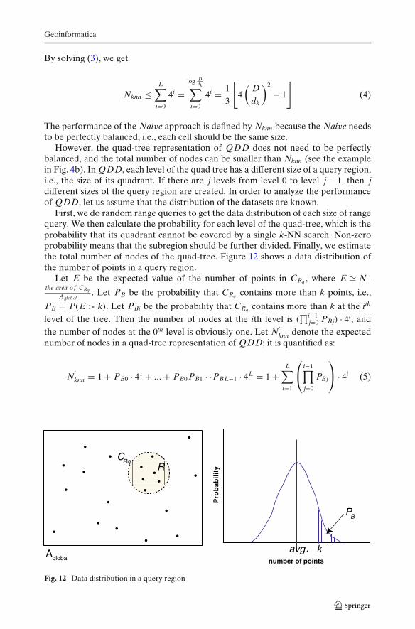
By solving (3), we get

Nknn ≤L∑

i=0

4i =log D

dk∑

i=0

4i = 1

3

[4

(Ddk

)2

− 1

](4)

The performance of the Naive approach is defined by Nknn because the Naive needsto be perfectly balanced, i.e., each cell should be the same size.

However, the quad-tree representation of QDD does not need to be perfectlybalanced, and the total number of nodes can be smaller than Nknn (see the examplein Fig. 4b). In QDD, each level of the quad tree has a different size of a query region,i.e., the size of its quadrant. If there are j levels from level 0 to level j − 1, then jdifferent sizes of the query region are created. In order to analyze the performanceof QDD, let us assume that the distribution of the datasets are known.

First, we do random range queries to get the data distribution of each size of rangequery. We then calculate the probability for each level of the quad-tree, which is theprobability that its quadrant cannot be covered by a single k-NN search. Non-zeroprobability means that the subregion should be further divided. Finally, we estimatethe total number of nodes of the quad-tree. Figure 12 shows a data distribution ofthe number of points in a query region.

Let E be the expected value of the number of points in CRq , where E N ·the area of CRq

Aglobal. Let PB be the probability that CRq contains more than k points, i.e.,

PB = P(E > k). Let PBi be the probability that CRq contains more than k at the ith

level of the tree. Then the number of nodes at the ith level is (∏i−1

j=0 PBj) · 4i, andthe number of nodes at the 0th level is obviously one. Let N

′knn denote the expected

number of nodes in a quad-tree representation of QDD; it is quantified as:

N′knn = 1 + PB0 · 41 + ... + PB0 PB1 · ·PBL−1 · 4L = 1 +

L∑

i=1

⎛

⎝i−1∏

j=0

PBj

⎞

⎠ · 4i (5)

Aglobal

CRq

number of points

Pro

bab

ilit

yR

avg. k

PB

Fig. 12 Data distribution in a query region

Geoinformatica

Table 2 Statistical analysis of QDD: 4K synthetic uniformly distributed data set

Level Query size PBi (%) k = 5 10 15 20 30 40 50

Level 0 3% PB0 100 100 100 100 100 100 100Level 1 1/41· 3% PB1 100 100 99.96 96.27 50.00 3.73 0Level 2 1/42· 3% PB2 54.48 45.52 6.35 0 0 0 0Level 3 1/43· 3% PB3 36.94 0 0 0 0 0 0Level 4 1/44· 3% PB4 0 0 0 0 0 0 0Number of Nknn 341 85 85 85 21 21 5k-NN N

′knn 108 51 26 21 13 6 5

searches QDD 115 59 29 25 16 7 3

Since PBi ≤ 1 for every level i,∏i−1

j=0 PBj becomes smaller and smaller as the treelevel increases, and finally approaches 0. Therefore, N

′knn ≤ Nknn.

Table 2 shows the analysis of QDD for our 4K synthetic uniformly distributeddata set. The quad tree for the 4K data set has six levels from level 0 to 5.Each probability PBi for level i is calculated based on the data distribution of thegiven range query. We compare N

′knn with Nknn as well as with the results of the

QDD algorithm. For example, when k = 15, a quadrant at level 1 is not covered bya single k-NN search with a 99.96% probability, and one at level 2 is not coveredby a k-NN search with a 6.35% probability. The perfect quad-tree with four levelshas 85 nodes in total. Therefore, the total number of k-NN calls for the Naiveapproach is Nknn = 85 while N

′knn = 26 for this case. The number of k-NN calls with

QDD for this example was 29 as presented in Section 5.3. Overall, N′knn had 62% of

average reduction compared to Nknn. We also observed that the maximum differencebetween QDD and N

′knn was 9%. This statistical analysis describes the behavior of

the QDD algorithm.QDD discards the returned k-NN result when the k-NN circle does not cover the

given query region and repeatedly calls additional four k-NN searches for the newfour subregions. Thus, we can consider skipping some levels of the QDD processto reduce unnecessary calls. If Rc is the current query region of a k-NN search, andPs is the probability that the k-NN circle completely covers Rc, then 1 − Ps is theprobability that the k-NN circle fails to cover the region. From statistical analysisbased on the results of the previous k-NN searches, we estimate the probability Ps

that the k-NN search covers Rc. To skip the current call of k-NN search, the totalexpected number of k-NN searches for the current level and the next level must begreater than four calls; four k-NN searches are required if we skip the current leveland directly go to four subregions for the next level. Hence we obtain the condition ofPs by the following equation: Ps + (1 − Ps) > 4. Therefore, QDD can skip a k-NNsearch for Rs iff Ps < 1

4 .

5.3 Experimental evaluation

5.3.1 Results of the DB algorithm

With the statistical knowledge of the data set, DB can decide the k value tominimize the number of k-NN calls. As a result, DB completed any range queryin one or two k-NN calls in all experiments with both synthetic and real datasets. The impact of ε was quantified by measuring the required number of k-

Geoinformatica

0%

20%

40%

60%

80%

100%

120%

epsilon value

perc

enta

ge o

f ran

ge q

uerie

s

1 k-NN call on uni. 4k

2 k-NN calls on uni. 4k

1 k-NN call on exp. 4k

2 k-NN calls on exp. 4k

(a) 4k Synthetic data set with 3% region queries

0%

20%

40%

60%

80%

100%

120%

1 1.2 1.4 1.6 1.8 21 1.2 1.4 1.6 1.8 2epsilon value

perc

enta

ge o

f ran

ge q

uerie

s

1 k-NN call

2 k-NN calls

(b) Real data set with 3% region queries

Fig. 13 Percentage of k-NN calls of DB(a, b)

NN calls while varying ε. As ε increased from 1.0 to 2.0, more range querieswere completed in a single k-NN call. Figure 13a shows what percentage ofrange queries were evaluated in one k-NN call (or in two) while varying ε. Forexample, in the case of the uniformly distributed dataset, when ε = 1.0, 57%of range queries were covered by one k-NN search while 43% were by two k-NN searches. When ε ≥ 1.2, all range queries were completed in one k-NN call.Overall, the exponential data set required a higher number of k-NN calls thanthe uniform data. The real data set showed a similar trend as the exponentialdata set.

DB performed all range queries in one or two k-NN calls with over-estimatedvalues of k. Because DB uses a loosely bounded k value, the obtained k-NN circleCr is larger than CRq in most cases. To quantify how accurately DB estimates Cr

with regard to CRq (Cr/CRq or r/Rq) using ε, we measured the ratio of r to Rq whilevarying ε (Fig. 14). The ratio was approximately 1.26 and 1.98 for the uniform andexponential data sets, respectively, when ε = 1.5 while the ratio was 1.48 for theuniform data set and 2.34 for the exponential data set when ε = 2.0. The ratio for

0.0

1.0

2.0

3.0

4.0

5.0

1% 2% 3% 4% 5% 6% 7% 8% 9% 10%

size of range query

Acc

urac

y (r

/Rq)

exp. e=2.0

uniform e=2.0

exp. e=1.5

uniform e=1.5

(a) 4k Synthetic data set with 3% region queries

0.0

1.0

2.0

3.0

4.0

5.0

1% 2% 3% 4% 5% 6% 7% 8% 9% 10%

size of range query

Acc

urac

y (r

/Rq)

epsilon = 2.0

epsilon = 1.5

(b) Real data set with 3% region queries

Fig. 14 Accuracy of DB(a, b)

Geoinformatica

0

20

40

60

80

100

120nu

mbe

r of

k-N

N c

alls

0

20

40

60

80

100

120

num

ber

of k

-NN

cal

ls

QDD w/uniform

DCDT w/uniform

N.C. w/uniform

(a) Uniformly distributed data set

5 10 15 20 25 30 35 40 45 50

value of k

5 10 15 20 25 30 35 40 45 50

value of k

QDD w/exponential

DCDT w/exponential

N.C. w/exponential

(b) Exponentially distributed data set

Fig. 15 Number of k-NN calls for 4K synthetic data set with 3% range query (a, b)

the real data set are presented in Fig. 14b: 1.51 with ε = 1.5 and 1.77 with ε = 2.0.For both the synthetic and real data sets, the ratio r to Rq decreased as the size of therange query increased.

5.3.2 Results of QDD and DCDT

First, we compared the performance of QDD and DCDT with the theoreticalminimum, i.e., the necessary condition (N.C.) � n

k�, where n is the number of points inR. Figure 15a and b show the comparisons of QDD, DCDT and N.C. with uniformlydistributed and exponentially distributed 4k synthetic data sets, respectively. Forboth DCDT and QDD, the number of k-NN calls rapidly decreased as the valueof k increased in the range 5-15 for uniformly distributed data and 5-10 for theexponentially distributed data. Then, it slowly decreased as the value of k becamelarger, approaching to those of N.C. when k is over 35. The results for the realdata set have similar trends to those of the exponentially distributed syntheticdata set (Fig. 16). Note that k is determined not by the client but by the Webinterface, and a typical k value in real applications ranges between 5 and 20 [4].In both synthetic and real data sets, DCDT needed a significantly smaller numberof k-NN calls compared to QDD. For example, with the exponential data set(4K), DCDT showed 55.3% of average reduction in the required number of k-

Fig. 16 Number of k-NN callsfor real data set with 3% rangequery

0

20

40

60

80

100

120

140

5 10 15 20 25 30 35 40 45 50

k value

num

ber

of k

-NN

cal

ls

QDD

N.C.

QDD

DCDT

N.C.

Geoinformatica

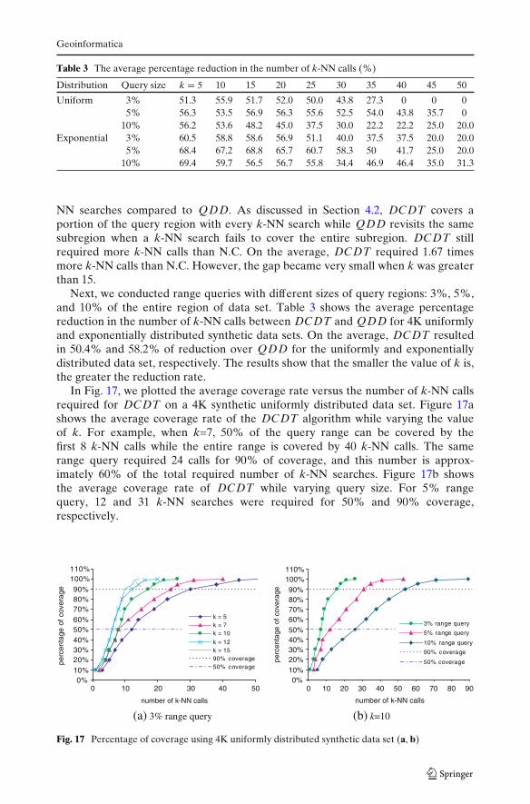
Table 3 The average percentage reduction in the number of k-NN calls (%)

Distribution Query size k = 5 10 15 20 25 30 35 40 45 50

Uniform 3% 51.3 55.9 51.7 52.0 50.0 43.8 27.3 0 0 05% 56.3 53.5 56.9 56.3 55.6 52.5 54.0 43.8 35.7 0

10% 56.2 53.6 48.2 45.0 37.5 30.0 22.2 22.2 25.0 20.0Exponential 3% 60.5 58.8 58.6 56.9 51.1 40.0 37.5 37.5 20.0 20.0

5% 68.4 67.2 68.8 65.7 60.7 58.3 50 41.7 25.0 20.010% 69.4 59.7 56.5 56.7 55.8 34.4 46.9 46.4 35.0 31.3

NN searches compared to QDD. As discussed in Section 4.2, DCDT covers aportion of the query region with every k-NN search while QDD revisits the samesubregion when a k-NN search fails to cover the entire subregion. DCDT stillrequired more k-NN calls than N.C. On the average, DCDT required 1.67 timesmore k-NN calls than N.C. However, the gap became very small when k was greaterthan 15.

Next, we conducted range queries with different sizes of query regions: 3%, 5%,and 10% of the entire region of data set. Table 3 shows the average percentagereduction in the number of k-NN calls between DCDT and QDD for 4K uniformlyand exponentially distributed synthetic data sets. On the average, DCDT resultedin 50.4% and 58.2% of reduction over QDD for the uniformly and exponentiallydistributed data set, respectively. The results show that the smaller the value of k is,the greater the reduction rate.

In Fig. 17, we plotted the average coverage rate versus the number of k-NN callsrequired for DCDT on a 4K synthetic uniformly distributed data set. Figure 17ashows the average coverage rate of the DCDT algorithm while varying the valueof k. For example, when k=7, 50% of the query range can be covered by thefirst 8 k-NN calls while the entire range is covered by 40 k-NN calls. The samerange query required 24 calls for 90% of coverage, and this number is approx-imately 60% of the total required number of k-NN searches. Figure 17b showsthe average coverage rate of DCDT while varying query size. For 5% rangequery, 12 and 31 k-NN searches were required for 50% and 90% coverage,respectively.

0%10%20%30%40%50%60%70%80%90%

100%110%

0 10 20 30 40 50

number of k-NN calls

perc

enta

ge o

f co

vera

ge

k = 5k = 7k = 10

k = 12k = 1590% coverage50% coverage

(a) 3% range query

0%10%20%30%40%50%60%70%80%90%

100%110%

0 10 20 30 40 50 60 70 80 90

number of k-NN calls

perc

enta

ge o

f co

vera

ge

3% range query

5% range query

10% range query

90% coverage

50% coverage

(b) k=10

Fig. 17 Percentage of coverage using 4K uniformly distributed synthetic data set (a, b)

Geoinformatica

0%

10%

20%

30%

40%

50%

60%

70%

80%

90%

100%

110%

0 10 20 30 40 50

number of k-NN calls

0 10 20 30 40 50 60 70 80 90

number of k-NN calls

perc

enta

ge o

f cov

erag

e

k = 5k = 7k = 10

k = 12k = 1590% coverage50% coverage

(a) 3% range query

0%10%20%30%40%50%60%70%80%90%

100%110%

perc

enta

ge o

f cov

erag

e

3% range query

5% range query

10% range query

90% coverage

50% coverage

(b) k=10

Fig. 18 Percentage of coverage using real data set (a, b)

Figure 18a and b show the average coverage rate versus the number of k-NN calls required for DCDT on real data set while varying the value of k in(a) and varying query size in (b). When k=7, 50% of the query range can becovered by 20% of the total required number of k-NN searches. The same rangequery required 16 calls for 90% of coverage, which is 55% of the total requirednumber of k-NN searches. For 5% range query, 20% and 58% of the total re-quired k-NN searches were required to cover 50% and 90% of the query range,respectively.

6 Conclusions

In this paper, we introduced the problem of evaluating spatial range queries onthe web data by using only k-Nearest Neighbor searches. The problem of findinga minimum number of k-NN searches to cover the query range appears to be hardeven if the locations of the objects (points) are known.

Based on the classification of k-NN interfaces, four algorithms were proposed toachieve the completeness and efficiency requirements of spatial range queries. QuadDrill Down (QDD) and Dynamic Constrained Delaunay Triangulation (DCDT)algorithms were proposed for the case where we have no knowledge about thedistribution of the data sets with the most restricted k-NN interface (i.e., no controlon the value of k). We showed that both QDD and DCDT can cover the entirerange even with the most restricted environment while providing reasonable per-formance. The efficiency of the algorithms were measured using statistical analysisand empirical experiments. DCDT provides a better performance than QDD. Inthe presence the data distribution knowledge and more flexible k-NN interface, weproposed the DB algorithm that can support any range query with only one ortwo k-NN searches as was demonstrated in all our experiments. The Hybrid (HB)algorithm provides the possibility of customization of our algorithms for real worldapplications.

We plan to expand our range query algorithms for parallel k-NN searches onmultiple web site, which is expected to significantly enhance the data integration and

Geoinformatica

search time. Consequently, a new problem of minimizing the overlapping area canbe introduced.

Acknowledgements The authors thank Prof. Petr Vojtechovský for providing helpful suggestionsand Brandon Haenlein for the valuable discussions throughout this work.

References

1. Barish G, Chen Y, Dipasquo D, Knoblock CA, Minton S, Muslea I, Shahabi C (2000) Theaterloc:using information integration technology to rapidly build virtual application. In: Proceedingsof international conf. on data engineering (ICDE), 28 February–3 March 2000, San Diego,pp 681–682

2. Bae WD, Alkobaisi S, Kim SH, Narayanappa S, Shahabi C (2007) Supporting range queries onweb data using k-nearest neighbor search. In: Proceedings of the 7th international symposium onweb and wireless GIS (W2GIS 2007), 28–29 November 2007, Cardiff, pp 61–75

3. Bae WD, Alkobaisi S, Kim SH, Narayanappa S, Shahabi C (2007) Supporting range queries onweb data using k-nearest neighbor search. Technical report DU-CS-08-01, University of Denver

4. Byers S, Freire J, Silva C (2001) Efficient acquisition of web data through restricted queryinterface. In: Poster proceedings of the world wide web conference (WWW10), Hong Kong, 1–5May 2001, pp 184–185

5. Chew LP (1989) Constrained Delaunay triangulations. Algorithmica 4(1):97–1086. Dickerson M, Drysdale R, Sack J (1992) Simple algorithms for enumerating interpoint distances

and finding k nearest neighbors. Int J Comput Geom Appl 2:221–2397. Eppstein D, Erickson J (1994) Interated nearest neighbors and finding minimal polytypes.

Discrete Comput Geom 11:321–3508. Gaede V, Gounter O (1998) Multidimensional access methods. ACM Comput Surv 30(2):

170–2319. Hieu LQ (2005) Integration of web data sources: a survey of existing problems. In: Proceedings

of the 17th GI-workshop on the foundations of databases (GvD), Wörlitz, 17–20 May 200510. Liu D, Lim E, Ng W (2002) Efficient k nearest neighbor queries on remote spatial databases using

range estimation. In: Proceedings of international conf. on scientific and statistical databasesmanagement (SSDMB), Edinburgh, 24–26 July 2002, pp 121–130

11. Mergerian S, Koushanfar F (2005) Worst and best-case coverage in sensor networks. IEEE TransMob Comput 4(1):84–92

12. Nie Z, Kambhampati S, Nambiar U (2005) Effectively mining and using coverage and overlapstatistics for data integration. IEEE Trans Knowl Data Eng 17(5):638–651, May

13. Roussopoulos N, Kelley S, Vincent F (1995) Nearest neighbor queries. In: Proceedings of ACMSIGMOD, San Jose, May 1995, pp 71–79

14. Samet H (1985) Data structures for quadtree approximation and compression. Commun ACM28(9):973–993, September

15. Sharifzadeh M, Shahabi C (2006) Utilizing voronoi cells of location data streams for accuratecomputation of aggregate functions in sensor networks. GeoInformatica 10(1):9–36

16. Song Z, Roussonpoulos N (2001) K-nearest neighbor search for moving query point. In: Proceed-ings of international symposium on spatial and temporal databases (SSTD), Redondo Beach,12–15 July 2001, pp 79–96

17. Tao U, Zhang U, Papadias D, Mamoulis N (2004) An efficient cost model for optimization ofnearest neighbor search in low and medium dimensional spaces. IEEE Trans Knowl Data Eng16(10):1169–1184, October

18. USGS (2001) USGS mineral resources on-line spatial data. http://tin.er.usgs.gov/19. Wang G, Cao G, Porta TL (2003) Movement-assisted sensor deployment. In: Proceedings of

IEEE INFOCOM, San Francisco, 30 March–3 April 2003, pp 2469–247920. Wang S, Armstrong MP (2003) A quadtree approach to domain decomposition for spatial

interpolation in grid computing environments. Parallel Comput 29(3):1481–1504, April21. Wu C, Lee K, Chung Y (2006) A Delaunay triangulation based method for wireless sensor

network deployment. In: Proceedings of ICPADS, Minneapolis, July 2006, pp 253–26022. Yerneni R, Li C, Garcia-Molina H, Ullman J (1999) Computing capabilities of mediators. In:

Proceedings of SIGMOD, Philadelphia, 1–3 June 1999, pp 443–454

Geoinformatica

Wan D. Bae is currently an assistant professor in the Mathematics, Statistics and Computer ScienceDepartment at the University of Wisconsin-Stout. She received her Ph.D. in Computer Sciencefrom the University of Denver in 2007. Dr. Bae’s current research interests include online queryprocessing, Geographic Information Systems, digital mapping, multidimensional data analysis anddata mining in spatial and spatiotemporal databases.

Shayma Alkobaisi is currently an assistant professor at the College of Information Technologyin the United Arab Emirates University. She received her Ph.D. in Computer Science from theUniversity of Denver in 2008. Dr. Alkobaisi’s research interests include uncertainty managementin spatiotemporal databases, online query processing in spatial databases, Geographic InformationSystems and computational geometry.

Geoinformatica

Seon Ho Kim is currently an associate professor in the Computer Science & Information TechnologyDepartment at the University of District of Columbia. He received his Ph.D. in Computer Sciencefrom the University of Southern California in 1999. Dr. Kim’s primary research interests includedesign and implementation of multimedia storage systems, and databases, spatiotemporal databases,and GIS. He co-chaired the 2004 ACM Workshop on Next Generation Residential BroadbandChallenges in conjunction with the ACM Multimedia Conference.

Sada Narayanappa is currently an advanced computing technologist at Jeppesen. He receivedhis Ph.D. in Mathematics and Computer Science from the University of Denver in 2006. Dr.Narayanappa’s primary research interests include computational geometry, graph theory, algo-rithms, design and implementation of databases.

Geoinformatica

Cyrus Shahabi is currently an Associate Professor and the Director of the Information Laboratory(InfoLAB) at the Computer Science Department and also a Research Area Director at the NSF’sIntegrated Media Systems Center (IMSC) at the University of Southern California. He receivedhis Ph.D. degree in Computer Science from the University of Southern California in August 1996.Dr. Shahabi’s current research interests include Peer-to-Peer Systems, Streaming Architectures,Geospatial Data Integration and Multidimensional Data Analysis. He is currently on the editorialboard of ACM Computers in Entertainment magazine. He is also serving on many conferenceprogram committees such as ICDE, SSTD, ACM SIGMOD, ACM GIS. Dr. Shahabi is the recipientof the 2002 National Science Foundation CAREER Award and 2003 Presidential Early CareerAwards for Scientists and Engineers (PECASE). In 2001, he also received an award from the OkawaFoundations.