T

WEATHER IN RELATION TO

PHYSICAL

CHARACTERISTICS

All of the matter and energy in the physical and biological system in which we live has, theoretically, potential ecological significance. Of greatest interest to the ecologist is the matter and energy distribution within the earth-atmosphere interface, or biosphere, which supports life. Most of this energy originates outside of the atmosphere, such as the radiant energy from the sun. Some comes from within the earth; geothermal energy is an example. The analytical ecologist is interested in the physical and biological interaction between matter and energy in the biosphere. Before analyzing some of these interactions, let us review both the relationships between the sun and earth and the weather in relation to physical characteristics at the earth's surface.

5-1 THE DISTRIBUTION OF SUNLIGHT

One of the more precise physical relationships in the universe is the position of the sun relative to the earth. This precision is manifested by the regularity with which the earth revolves around the sun and rotates on its axis. The calendar does not represent this relationship perfectly; the addition of a day in February every four years is a correction factor for this.

The ecological role of sunlight is significant. Different day lengths affect the growth and reproduction of plants and animals. Sunlight generates different thermal relationships in the atmosphere that result in weather patterns. It is a source of energy for the process of photosynthesis upon which all life depends. It alters the thermal regime at the earth' s surface, causing changes in physical conditions as well as in the behavior of plants and animals. Many more effects

57

u

58 WEATH ER AN D PHYSICAL CHARACTER ISTICS

can also be recognized, of course. Before considering its effect on plants and

animals, let us consider how it is related to physical characteristics on the earth, such as topography over daily and seasonal time periods.

The times at which the sun rises and sets for different latitudes are available in tabular form. Differences within a one-hour time zone can be corrected for in order to determine solar time. Such tables are not suitable for direct entry into a computer program. Sunrise and sunset times can be calculated on the basis of the spatial relationships between the sun and earth, however. An equation can be used to store this information in a computing system, which can then calculate

the times at which the sun rises and sets, the length of daylight, and other solar considerations in an ecological analysis .

The sunrise time, sunset time, hours of daylight, altitude of the sun at solar noon, and the solar insolation in langleys per minute for any slope aspect, slope angle, and time can be calculated from inputs of date (Julian Calendar), latitude,

slope aspect, slope angle, time of day (0 to 2400 hours), and transmittance of the atmosphere (Robbins, unpublished data, BioThermal Laboratory).

A similar type of program that calculates additional factors pertaining to the spectral characteristics of radiation has been described by McCullough and Porter (1971) . Their program generates clear-day direct and diffuse components of

natural terrestrial radiation for any time of the day, elevation, terrestrial latitude, and time of year. It computes radiation spectra for large zenith angles in which atmospheric curvature and refraction are important, irradiation patterns at lati­tudes > 66 ° 30' (polar zones), the variation of the diffused spectral components of solar radiation with the elevation and reflectivity of the underlying surface, and diffused ultraviolet radiation spectra where ozone absorption of the scattered radiation must be accounted for. These outputs are generated from eight inputs, including time of day, day of year, latitude, longitude, sea level, meteorological range (visibility), atmospheric pressure (i.e., elevation), reflectivity of the under­lying earth's surface, and total precipitable water vapor.

There are data in the literature that are useful in evaluating the outputs of these two programs . Sellers (1965), for example, shows the distribution of solar

radiation throughout the United States at different times of the year (Figure 5-1).

Variations in the radiation values shown are due to differences in latitude, altitude,

distribution of water, and topographical effects on weather patterns, and so forth . Note the large difference between January and June. O ther data are found in textbooks on meteorology and in numerous research reports in meteorological journals .

The outputs from these two programs are not perfect representations of these parameters at every point on the earth's surface. The programs are useful for setting an ecological "stage" with a few principal characters . The interactions between sunrise and sunset time, length of daylight, animal movements, breeding conditioI).s, plant productivity, thermal energy balance, and other significant components of the ecosystem might be considered initially. Since the eguipment necessary to make these fairly complex programs workable is seldom available to students, it is suggested that simpler approximations be made that can be

f

.r ).

:1.

m al

se or ns ng mt

2nt ble

be

5·1 DISTRIBUTION OF SUN LIGHT 59

B

FI GURE 5-1. The average solar radiation on a horizontal surface in the United

States in (A) January and (B) July. The units are langleys per day. (From Sellers 1965.)

60 WEATHER AND PH YSICAL CHARACTER ISTICS

2.0

1.5

::: .§ June 21

2-1.0

Sept 21 and Mar 21

0 .5

0 ~ ____ -L-ll~L-____ L-____ ~~~ ____ ~

Sunrise Solar noon Sunset

FIGURE 5-2. Sunrise, sunset, and solar radia tion values for a latitude of 42° 26' N (Ithaca, N.Y.). The dashed

lines are linear approximations of the radiation curve

(see text) .

24

handled by desk-top computing systems or calculators, or can even be done • without the aid of a machine. For example, solar radiation curves can be approxi­mated by a linear regression equation (Figure 5-2). This obviously results in potentially large errors. The student of analytical ecology is urged to consider the interreactions between solar radiation and an organism, however, and the linear approximation is quite adequate for working out the mechanisms of a predictive solar radiation curve in relation to the biological response of an orga­nism. In other words, extensive detail in part of the total organism-environment ' relationship is undesirable until all parts of the relationship have been considered.

THE ATMOSPHERE . The atmosphere is divided into several general regions (Figure 5-3). These include the troposphere, the stratosphere, the mesosphere, the thermo­sphere, and the exosphere. The troposphere contains the "weather" and shows a general decrease in temperature with height. Its upper limit is characterized by the maximum height of most clouds and storms. The stratosphere has a fairly complex temperature structure that varies geographically and seasonally. It also has wind regimes that vary seasonally and affect weather conditions at the earth's surface.

Above the stratosphere is the mesosphere, characterized by cold temperatures and very low atmospheric pressure. Above the mesosphere is the thermosphere in

which theoretical radiant temperatures rise with height, although artificial satellites do not acquire such temperatures because of the rarefied air (Barry and Chorley 1970). The thermosphere includes the region in which ultraviolet radiation and

:r

.e a

:\­

nt d.

Lre 10-

3 a

by irly 1150

th's

lres °e in lites .dey and

5·1 DISTR IBUTION OF SUN LIGHT 61

cosmic rays cause ionization; this region is called the ionosphere. The outer limits of the atmosphere grade into a region called the exosphere, or outer space, with its almost total lack of atoms. The earth's magnetic field becomes more important than gravity in the distribution of atomic particles in the exosphere. A more detailed discussion of the characteristics of the atmosphere may be found in Barry and Chorley (1970) .

All of the layers of the atmosphere are of interest to the ecologist since together they form the total blanket of air in the biosphere. The atmospheric components serve particular functions, including the filtering of radiant energy from the sun, insulation from heat loss at the earth's surface, and stabilization of weather and climate owing to the heat capacity of the air. Several cycles are present that relate to the movement of matter between an organism and its environment. These include the water cycle, the carbon cycle, the nitrogen cycle, the phosphorus cycle, and others.

Gases in the atmosphere include nitrogen, oxygen, argon, carbon dioxide, and water vapor, along with traces of several other elements. Oxygen is necessary for most forms of life, but other forms exist only in an anaerobic environment. In terms of quantity, carbon dioxide is the most variable of these gases. Consid­erations have been made for the enrichment of the atmosphere (carbon dioxide ferti lization) to promote plant growth. These are discussed in Chapter 15. Water vapor condenses in the atmosphere, resulting in precipitation. Its effect on the distribution of plants and animals is obvious on both a small and a large scale. Precipitation limits visibility, too, so observations of animals are more difficult and field work is less efficiently carried out in rain or snow. Consequently, information on animals in storms is lacking, yet these extreme conditions may affect their survival and productivity.

E ~

~ 00 OJ :r:

The ionosphere is affected by magnetic storms on the sun, with an increase

100

80

60

40

20

a

Exosphere (;:;,; 500 km)

Thermosphere

Ionizing region

Mesosphere

Stratosphere

Troposphere

FIGURE 5-3. Atmospheric layers; each grades into the next without a sharp line of demar­cation between them.

62 WEATHER AND PHYS'ICAL CHARACTERISTICS

in the number of free electrons present during periods of intense activity. Popula­tion cycles have been attributed to these storms and subsequent electrical activity in the ionosphere, although- there is considerable controversy over the validity of such correlations. Personal observations by the author indicate that white-tailed deer seem to respond to unidentified factors, with an increase in nervousness, activity, and physiological parameters such as heart rate. The possible interactions between the energy from the sun, cosmic rays, ionization in the thermosphere, electrical activity at ground level, and physiological processes in plants and animals need further analyses through basic investigations of atmospheric physics,

physiology, neurology, and behavior.

5-2 ATMOSPHERIC WATER

Atmospheric water is found in gaseous form or droplet form. The quantity of

water present in gaseous form is expressed as vapor pressure. When the vapor' pressure is maximum for the temperature of the atmosphere, the air is said to be saturated. Thus the maximum vapor pressure of the air is called its saturation

pressure, and the actual quanti ty of vap or present (vapor pressure) is a function of the temperature of the atmosphere. Relative humidity is equal to the vapor pressure divided by saturation pressure times 100. Students are reminded that relative humidity is temperature dependent , a fact often overlooked in ecological analysis. This will be discussed again in Chapter 6 .

Clouds form as condensation takes place around hygroscopic nuclei in the

atmosphere . These particles can be dust, smoke, sulphur dioxide, salts (NaCl), or similar microscopic substances (Barry and Chorley 1970). Clouds have distinct characteristics that are classified in an internationally adopted system according to the shape, structure, vertical height, and altitude of the cloud. Cloud types

can be identified through a "keying out" process similar to a taxonomic key for

plants and animals (Table 5-1). Clouds reflect and absorb solar radiation and are good absorbers and emitters of infrared radiation. They are also the centers of ,

considerable electrical activity, as well as the source of precipitation.

5-3 PRECIPITATION

Precipitation consists of all liquid and frozen forms of water, including rain, sleet, snow, hail, dew, hoarfrost, fog-drip, and rime (Barry and Chorley 1970). Rain

and snow are the only forms that contribute significantly to the precipitation totals, but some of the other forms, such as dew and hail, can have significant ecological impact. The analytical ecologist is interested in the functional relationships be­tween precipitation and organisms, and this demands an understanding of the energy an.d matter relationships , between them rather than the mere correlation of observed responses of organisms in different precipitation regimes .

RAIN. A basic analysis of the functional relationships between precipitation and organisms permits these mechanisms to be related to other interactions

TABLE 5-1 A KEY FOR THE IDENTIFICATION OF CLOUD FORMATIONS (Beginning with couplet number one, select the most appropriate choice and go to the numbered couplet indicated until a cloud formation has been identified.)

5-3 PRECIPITATI ON 63

1 Clouds piled up, puffy, currents . .. .. -Clouds formed without vertical movement

2 Clouds, puffy, changing shape Strong vertical development .

3 Cloud veils or sheets

2

3

. cumulus, 13 . cumulonimbus, 15

..... 4

More or less broken. 4 Large halo present . .

No halo effect .

.. ___ . 7

. cirrostratus . .. 5

5 Sun visible through veil. . altostratus, 12 Sun not visible, heavy veil. . 6

6 Low uniform sheet, no ra in ... stratus Low heavy sheet, rain streaks. nimbostratus

7 High ice clouds, usually thin wispy streaks. . cirrus, 16 Heavier clouds, patchy or irregular masses _ 8

8 Patches or layers of puffy or roll - like gray or whitish clouds, corona often . . . . . . . . . . . . . 9 Irregular masses in a rolling or puffy layer, gray with darker shading stratocumulus, 18

9 White to light gray roll-like, or roll-like in combination with patchy or wispy, high ice clouds . . . . . . .. . . .. .. . .... . . . . cirrocumulus Patches or layers of puffy or roll-like gray or whitish clouds, corona often, middle water and ice clouds . . . . . . . . altocumulus, 10

10 White to gray roll-like middle water and ice clouds . . . . ..... 11 Patchy to nearly continuous gray middle water and ice clouds . . . . . . . . . . . . . . . . . . . . . . . .. altocumulus perlucidus

11 White to light gray clouds, roll-like or less distinctly so . . . . . . . ..... . . . . . . .... altocumulus translucidus Gray, roll-like clouds . . . . . . . . altocumulus translucidus undulatus

12 Darker clouds, but sun appears to be behind frosted glass. ....... .. ...... . . . . . . . . . . . altostratus opacus Lighter clouds, sun appears to be behind frosted glass . altostratus translucidus

13 Irregular patches broken by strong winds . . . . .cumulus fractus Bulky patches, white to gray . . .. 14

14 White to light gray, low water clouds, may be towering. . . . . . . . . . . . cumulus humilis Darker gray low water clouds, becoming more dense. . . . . . . . . . . . . . . . . . cum ulus congestus

15 Low vertical water clouds to towering water to ice clouds, often anvil shaped .. . . cumulonimbus capillatus Dense clouds with vertical development indicated by ventral projections, seldom seen . . . cumulonimbus capillatus mammatus

16 Thin wispy streaks, broken pattern . . . . . . . . . . . ... . . .. 17 Heavier streaks, almost patches, white, high ice clouds cirrus densus

17 Streaks broken, not spreading over sky . cirrus filosus Streaks broken, spreading over sky. . . cirrus cinus

18 Low water clouds, light gray. stratocumulus translucidus Low water clouds, dark gray . . . . . . . . stratocumulus opacus

64 WEATHER AN D PHYSICAL CHARACTERI STICS

Rainfall of X cm hc1 - - - __ Particle size----- Rate of fall----- (1)

(1) Raindrop inertia-Throughfa ll in canopies of different densities-(2)

(2) Rainfall reaching the soil surface~ Soil abSOrptiOn~ (3)

SoH ,""-off ~(') (5)

(3) Uptake of water by Plants~ Water available for Photosynthe.siS-(6)

(4) Percolation into soil Transpiration and evaporation

(5) Evaporation from soil surface/

(6) Gross energy produced by plants- Net energy for production by consumers

FIGURE 5-4. A flow sheet showing the relationships between rainfall per

hour, raindrop characteristics, soil absorption, plant productivity, and

consumer energy for production.

between organisms and environment. This is illustrated in Figure 5-4, in which the amount of rainfall in cm hc I is the beginning point for calculating the mass transport of water within a plant community, relating this movement to the feedback interactions between evaporation from the surface of the soil and evapotranspiration and to plant production.

FIGURE 5-5. There is a predictable relationship be­tween rainfall intensity and the diameter of the rain­

drops. (Data from Barry and Chorley 1970.)

16

Log, Y = -4.531 + 23 .124X (5-1)

12

-::--

..c E

..!:::. 8

'" ...... <= .;;;

c.::

4

o~~-----+--~=---~------~------~ .1 .2 .3 .4

Raindrop diameter (cm)

5-3 PRECIPITATION 65

How can the flow sheet in Figure 5-4 be useful? What kinds of relationships exist that make such an analysis work? Some basic data have been reported by

meteorologists that can be used to develop a series of calculations representing the relationships between rainfall in cm hr -1 and subsequent soil water, plant uptake of water, evapotranspiration, and plant production. For example, there is a relationship between precipitation intensity and raindrop size; a greater amount of rainfall per unit time is more dependent on the size of the raindrops than on the number of raindrops. Barry and Chorley (1970) point out that the most frequent diameter of drops in a rainfall of 0.1 cm hc1 is 0.1 cm; in 1.3 cm hr-1

it is 0 .2 cm; and in 10.2 cm hc1 it is 0.3 cm. These data can be expressed in equation form [equation (5-1) in Figure 5-5]. This relates to the number/ volume ratio of drops, too, as a drop having a diameter of 0.1 cm has a volume of 0.000524 cc, and 19,083,970 drops are necessary for 1 cm of water to cover an area of one square meter. This is a volume of 10 liters .

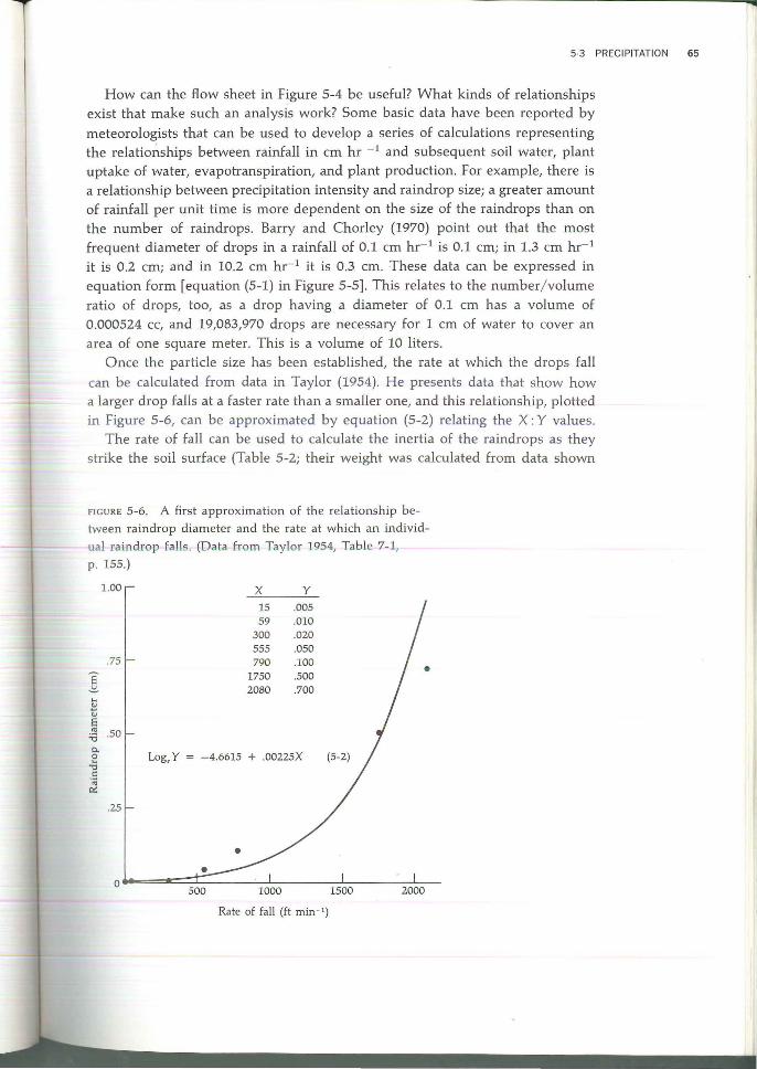
Once the particle size has been established, the rate at which the drops fall

can be calculated from data in Taylor (1954). He presents data that show how a larger drop falls at a faster rate than a smaller one, and this relationship, plotted in Figure 5-6, can be approximated by equation (5-2) relating the X: Y values.

The rate of fall can be used to calculate the inertia of the raindrops as they strike the soil surface (Table 5-2; their weight was calculated from data shown

FIGURE 5-6. A first approximation of the relationship be­

tween raindrop diameter and the rate at which an individ­

ual ra indrop falls _ (Data from Taylor 1954, Table 7-1,

p . ISS.)

1.00 x y

15 .005 59 .010

300 .020 555 .050 790 .100 • 1750 .500

_75

E ~ 2080 .700

I-;

~ ., E .. _50 :.a p" 0 1-0

Log, Y = -4_6615 + _00225X ."

c:: ;; ..:

.25

500 1000 2000

Rate of fall (ft min- I)

L

66 WEATHER AND PHYSICAL CHARACTERISTICS

TABLE 5-2 THE INERTIA OF INDIVIDUAL RA INDROPS AT DIFFERENT

RAINFALL INTENSITY

Inertia: Raindrop Raindrop Weight

Ra infall Diameler Raindrop Weighl Rale of Fall (g) X Rale (em hr-1) (em) (X 10- 3 g) ([I min- I) of Fall ([I min-i)

0.1 0.096 0.46 1031.96 0 .478 0 .2 0 .126 1.05 1152.33 1.207

0.3 0.144 1.56 1210.09 1.891 0.4 0.156 1.99 1246.95 2.479

0.5 0.166 2.40 1273.57 3.050 1.0 0.196 3.94 1347.37 5.312 1.5 0 .213 5.06 1385.46 7.010 2.0 0.226 6.04 1410.63 8.526 2.5 0.236 6.88 1429.22 9.836 3.0 0.243 7.51 1443.85 10.847 4.0 0.256 8.78 1466.00 12.878 5.0 0.265 9.74 1482.45 14.445 6 .0 0.273 10.65 1495.46 15.932 7.0 0.280 11.49 1506.17 17.312 8.0 0 .286 12.25 1515.24 18.560 9.0 0.291 12.90 1523.08 19.652

10.0 0.296 13.58 1529.99 20.776

Note: The values in this table and all subsequent tables containing calcu lations may vary according to the computing system used and the arrangement oj program steps in relation to rounding of num· bers.

in Figure 5-5; specific gravity of water = 1.0), and this inertia is of major impor­tance in determining how much of the rainfall can penetrate a plant canopy (throughfall), how much reaches the soil surface, and the mechanical impact it has on the soil surface. The inertia can be related to throughfall if the mechanical ·

strength of the plant canopy is known. The inertia can be related to soil disturb­ance if the mechanical strength bf the soil surface is known. This depends on the distribution of particle size and density and the cohesiveness of the soil material.

RAINFALL IN RELATION TO SOIL AND TOPOGRAPHY. The results shown in Table

5-2 illustrate relationships between the amount of rainfall per hour and the inertia

with which the drops strike a surface. The equations representing the factors and forces in the model were combined into a computing program that results in the outputs shown in the table. It is an example of a "rainfall per hour" to "inertia of the drops" conversion.

Let us expand the previous model to include soil absorption characteristics.

Suppose that a rainfall of 1 .3 cm hr- 1 is occurring. These raindrops strike the surface of the soil at a velocity of 1372.14 ft min-1 (see Table 5-2). Suppose that

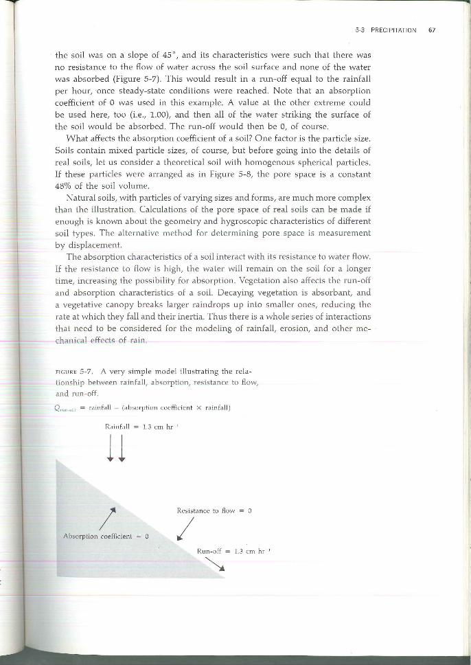
5-3 PRECIPITATION 67

the soil was on a slope of 45 0, and its characteristics were such that there was

no resistance to the flow of water across the soil surface and none of the water was absorbed (Figure 5-7). This would result in a run-off equal to the rainfall per hour, ·once steady-state conditions were reached. Note that an absorption coefficient of a was used in this example. A value at the other extreme could

be used here, too (i.e., 1.00), and then all of the water striking the surface of

the soil would be absorbed. The run-off would then be 0, of course. What affects the absorption coefficient of a soil? One factor is the particle size.

Soils contain mixed particle sizes, of course, but before going into the details of

real soils, let us consider a theoretical soil with homogenous spherical particles. If these particles were arranged as in Figure 5-8, the pore space is a constant 48% of the soil volume.

Natural soils, with particles of varying sizes and forms, are much more complex than the illustration. Calculations of the pore space of real soils can be made if enough is known about the geometry and hygroscopic characteristics of different soil types . The alternative method for determining pore space is measurement

by displacement. The absorption characteristics of a soil interact with its resistance to water flow.

If the resistance to flow is high, the water will remain on the soil for a longer time, increasing the possibility for absorption. Vegetation also affects the run-off

and absorption characteristics of a soil. Decaying vegetation is absorbant, and

a vegetative canopy breaks larger raindrops up into smaller ones, reducing the rate at which they fall and their inertia. Thus there is a whole series of interactions that need to be considered for the modeling of rainfall, erosion, and other me­chanical effects of rain.

FIGURE 5-7. A very simple model illustrating the rela­

tionship between rainfall, absorption, resistance to flow,

and run-off.

Q,u ,, -u rr = rainfall - (absorption coefficient X rainfall)

Rainfall = 1.3 cm hr - '

11

I Resistance to flow a

I Absorption coefficient = a

Run-off = 1.3 cm hr - '

•

I ,

68 WEATHER AN D PH YSICAL CHARACTER ISTICS

FIGURE 5-8. Spherical particles arranged in

the simplest geometry.

The main point thus far is the illustration of the logic of the model-building process, showing how to proceed from the very simple to the more complex, but limiting this complexity to that which is fully understood. Real values are not necessary for building the initial model since many limits can be recognized i_n the natural world. Resistance to water flow, for example, must vary from no resistance to complete resistance. The effect of this variation can be analyzed within those limits, and if there is a significant ecological effect, further analyses are necessary.

SNOW. Snow is an extremely important ecological force that performs many different functions . It reduces visibility when it falls; it is a mechanical barrier, a good insulator, a source of soil moisture, and a source of run-off water. Its many different functions as a physical material, coupled with its many different inter­actions with organisms, compels the analytical ecologist to consider it an important component of the ecosystem. It is an interesting component of analytical models because it has so many different functions. Let us consider its physical charac­teristics first and relate it to organisms in later chapters.

Ice-crystals are formed in the atmosphere at temperatures below freezing by the sublimation of water vapor on hygroscopic nuclei. The ice crystals take various shapes, dependent on atmospheric conditions at the time of crystallization. New­fallen snow generally has a low density (0.05-0.10 g cm-3) owing to the dendritic

structure of the crystals. Atmospheric temperature and wind are the two primary factors that alter the density of new-fallen snow. Snow density will increase an average of 0.0065 g cm-3 for each 1°C increase in surface air temperature at the time of deposition.

Reported density of new-fallen snow varies from 0.06 for calm conditions to 0.34 for snow deposited during. gale winds. Snow density increases to 0.2-0.4 g cm- 3 as the age of the snowpack increases. As each new layer of snow is deposited, its upper surface is subjected to the weathering effects of radiation, rain, and wind, and the action of percolating water and diffusing water vapor.

s l,

r.

5·4 SNOW COVER AND KINETI C EN ERGY 69

The original delicate crystals become coarse grains; a developed snowpack shows distinct layers characteristic of individual snow-storm deposits and weathering effects (US Army 1956; Nakaya 1954).

CONDUCTIVITY. Factors affecting the thermal conductivity of snow are: (1) the structural and crystalline character of the snowpack, (2) the degree of compaction, (3) the extent of ice planes, (4) the wetness, and (5) the temperature of the snow. Experimental work shows that the thermal properties of snow (specific heat, conductivity, and diffusivity) can be predicted from snow density measurements

(Table 5-3). Heat transfer in a natural snowpack is complicated by the simultaneous occur­

rence of many different heat-exchange processes. The water vapor condenses and yields its heat of vaporization (::::;0.600 kcal g-l) upon reaching a cold surface. Rain or meltwater freezes within the subfreezing layers and adds the heat of fusion (0.08 kcal g-l). These two processes tend to change and influence the conductivity and diffusivity of the snow throughout the pack and influence the heat transfer rates (U.s. Army 1956).

Temperature gradients in the snowpack are more pronounced in the winter than in the spring. When the snowpack reaches an isothermal condition at O°C, the heat energy is dissipated in melting the snow.

5·4 SNOW COVER IN RELATION TO KINETIC ENERGY

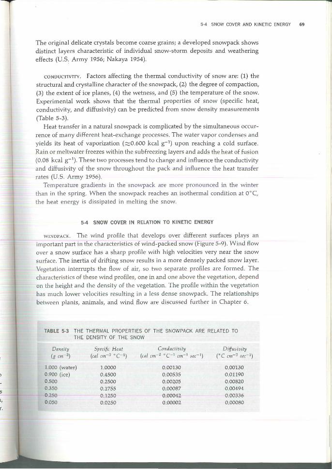
WINDPACK. The wind profile that develops over different surfaces plays an important part in the characteristics of wind-packed snow (Figure 5-9). W ind flow over a snow surface has a sharp profile with high velocities very near the snow surface. The inertia of drifting snow results in a more densely packed snow layer. Vegetation interrupts the flow of air, so two separate profiles are formed. The characteristics of these wind profiles, one in and one above the vegetation, depend on the height and the density of the vegetation. The profi le within the vegetation has much lower velocities resulting in a less dense snowpack. The relationships between plants, animals, and wind flow are discussed further in Chapter 6.

TABLE 5-3 THE THERMAL PROPERTIES OF THE SNOWPACK ARE RELATED TO THE DENSITY OF THE SNOW

Density Specific Hea t Conductivity Diffusivity (g cm-3) (cal cm- 3 ° C- l) (cal. cm-2 ° C- I cm- 1 5ec - 1) (OC cm-2 secI )

1.000 (water) 1.0000 0.00130 0.00130 0.900 (ice) 0.4500 0 .00535 0 .01190 0 .500 0 .2500 0.00205 0.00820 0 .350 0.1755 0 .00087 0 .00494 0 .250 0 .1250 0 .00042 0 .00336 0 .050 0 .0250 0 .00002 0.00080

I '

70 WEATHER AND PHYSICAL CHARACTER ISTICS

200 14 mi hr - '

175

150

125 Snow

E ~

.:c 100 0() Vegetation

'OJ :r:

75

Vegetation height

50

25

100 200 300 400 500 600 700

Wind velocity (em sec')

FIGURE 5-9. Vertical wind profiles over grass that is 60-70 cm in

height and over a snow surface.

THE EFFECT OF WINDBREAKS. The effect of windbreaks on the distribution of snow is well known, but the turbulent flow generated by windbreaks is often described

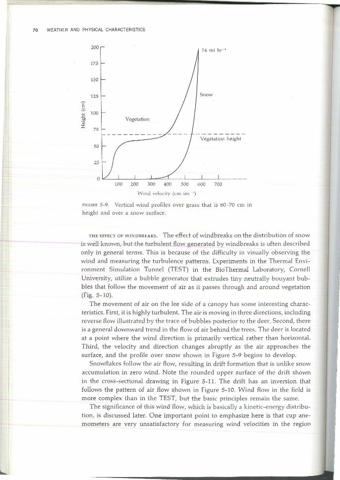
only in general terms. This is because of the difficulty in visually observing the wind and measuring the turbulence patterns. Experiments in the Thermal Envi­ronment Simulation Tunnel (TEST) in the BioThermal Laboratory, Cornell

University, utilize a bubble generator that extrudes tiny neutrally bouyant bub­bles that follow the movement of air as it passes through and around vegetation (Fig. 5-10).

The movement of air on the lee side of a canopy has some interesting charac­teristics. First, it is highly turbulent. The air is moving in three directions, including reverse flow illustrated by the trace of bubbles posterior to the deer. Second, there is a general downward trend in the flow of air behind the trees. The deer is located at a point where the wind direction is primarily vertical rather than horizontal. Third, the velocity and direction changes abruptly as the air approaches the surface, and the profile over snow shown in Figure 5-9 begins to develop.

Snowflakes follow the air flow, resulting in drift formation that is unlike snow accumulation in zero wind. Note the rounded upper surface of the drift shown

in the cross-sectional drawing in Figure 5-11. The drift has an inversion that follows the pattern of air flow shown in Figure 5-10. Wind flow in the field is more complex than in the TEST, but the basic principles remain the same.

The significance of this wind flow, which is basically a kinetic-energy distribu­

tion, is discussed later. One important point to emphasize here is that cup ane­mometers are very unsatisfactory for measuring wind velocities in the region

n

5-4 SNOW COVER AND K INETIC ENERGY 71

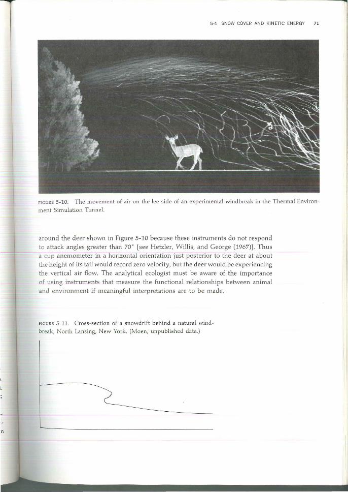
FIGURE 5-10. The movement of air on the lee side of an experimental windbreak in the Thermal Environ­

ment Simulation Tunnel.

around the deer shown in Figure 5-10 because these instruments do not respond to attack angles greater than 70° [see Hetzler, Willis, and George (1967)]' Thus a cup anemometer in a horizontal orientation just posterior to the deer at about

the height of its tail would record zero velocity, but the deer would be experiencing the vertical air flow. The analytical ecologist must be aware of the importance of using instruments that measure the functional relationships between animal and environment if meaningful interpretations are to be made.

FIGURE 5-11. Cross-section of a snowdrift behind a natural wind­

break, North Lansing, New York. (Moen, unpublished data .)

72 WEATHER AND PH YSICAL CHARACTERI STICS

SNOWFALL INTERCEPTION. The interception of falling snow by vegetative cover is an important factor when predicting snow accumulation on the ground, just as it is in predicting rainfall at the soil surface. The amount of interception varies greatly, depending on the type and density of the vegetation cover and the magnitude, intensity, and frequency of storms. High winds and intense solar radiation reduce the amount of snow trapped in the canopy. A moderately dense coniferous forest, in an area with an annual precipitation of 30-50 inches, may intercept 15%- 30% of the total winter precipitation. Equation (5-3) was developed for estimating the amount of interception in a coniferous tree stand in the north­western United States (U.s. Army 1956).

{~ercentag~ Of} = {0.36 X percentage} mterceptIon of canopy cover

(5-3)

THE ROLE OF SNOW IN A PRECIPITATION-CANOPV-SUBSTRATE MODEL. The amount of information about the structural, mechaniCal, and thermal characteristics of snow is quite adequate for assembling initial models of the role of snow in the ecology of different organisms. The equations for snow interception by different canopies and for conductivity of snow of different densities are important for determining the amount that reaches the ground's surface and its role as a mechanical barrier and an insulator against heat loss. Students are urged to develop models that permit calculations of these functions of snow. In the absence of real data that can be used to describe some of the functions, limits can still be recognized that serve the purpose of making first approximations. For example, the aging process of snow results in a continual change in snow density, and this in turn affects conductivity. The aging process is very dependent on radiation, wind, air temper­ature, and precipitation, and these are not readily predicted. Their effect, however, can be approximated since the lowest snow density possible is one limit and maximum density-ice-is the other. An initial model containing changes in snow density could include an equation that describes these changes purely as a function of time. The simplest format is a linear regression equation. Initial analyses can then begin with the philosophy "What if . .. ?", and the analytical ecologist uses the outputs from such considerations in determining the effect of such changes on the organism(s) in question. Once this has been done, it is desirable to go back to the first approximations and improve on them so they become more and more representative of real situations in the natural world.

THE EFFECT OF SNOW DISTRIBUTION ON ANIMALS. The distribution of snow is a

reflection of the distribution of kinetic energy in time and space. Animals are subject to these patterns and must be able to cope with them if they are to survive. High-density snowpacks can have opposite effects on animal life. They may pose a mechanical barrier, increasing the metabolic energy necessary for the animal to move through the snow. This is a cost to the animal that must be compensated for either by food ingested and metabolized or by reserves that have been built up during more favorable periods. Or the snowpack may be dense enough to support the weight of the animal, facilitating its movement. This results in the

5-4 SNOW COVER AND KINETIC ENERGY 73

conservation of energy and it may also place the animal within reach of a food supply that would otherwise be too high.

The mechanical characteristics of the snowpack have a direct effect on the thermal benefit it provides such birds as grouse, which roost in the snow on cold winter nights. If the birds can penetrate the snow, they will be in a thermal regime that is very different from one above the snow surface.

Snow accumulation may directly influence the amount of available food for a wild animal. For example, the vertical distribution of potential food for deer that browse in an upland hardwood community in the Connecticut Hill Game Management Area south of Ithaca, New York, is such that one foot of snow renders

97% of it available. The zone of invading plants between a hemlock stand and an abandoned field have quite a different vertical distribution of food . One foot of snow in that habitat reduced the food supply by 25%, and two feet of snow reduced it by 40%. The marked differences between these two types of habitats indicate that the effect of one foot of snow is dependent on the vertical distribution of food, so snow depths of one foot in each of the two stands are not ecological equivalents .

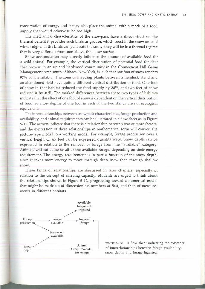
The interrelationships between snowpack characteristics, forage production and availability, and animal requirements can be illustrated in a flow sheet as in Figure 5-12. The arrows indicate that there is a relationship between two or more factors, and the expression of these relationships in mathematical form will convert the picture-type model to a working model. For example, forage production over a vertical height of six feet can be expressed quantitatively. Snow depth can be expressed in relation to the removal of forage from the "available" category. Animals will eat some or all of the available forage, depending on their energy requirement. The energy requirement is in part a function of the snow depth, since it takes more energy to move through deep snow than through shallow snow.

These kinds of relationships are discussed in later chapters, especially in relation to the concept of carrying capacity. Students are urged to think about the relationships shown in Figure 5-12, progressing toward a numerical model that might be made up of dimensionless numbers at first, and then of measure­ments in different habitats .

Available forage not

/ ingested

Forage • Forage • Ingested production available forage

~

snow/ depth

Forage not available

Animal • requirements

for energy

FIGURE 5-12. A flow sheet indicating the existence

of interrelationships between forage availability,

snow depth, and forage ingested.

74 WEATH ER AND PHYSICAL CHARACTER ISTICS

Since the model-building process is such a significant part of analytical ecology,

it is essential that students grasp the logic and philosophy sufficiently well to begin building meaningful models themselves. Let us turn our attention in the next chapter to weather and the processes of thermal exchange, with additional models that illustrate the process of model building and at the same time provide infor­mation on the distribution of thermal energy in the real world. Keep in mind that the process of analytical ecology results in an analysis that may be compared to dramatic art, moving from simple one-act ecological plays, each with just a

few principal characters, to the more comprehensive productions that approach greater and greater realism.

LI TERATU RE CITED IN CHAPTER 5

Barry, R. G., and R. J. Chorley. 1970. Atmosphere, weather, and climate. New York: Holt, Rinehart and Winston, 320 pp.

Hetzler, R. E., W. O. Willis, and E. J. George. 1967. Cup anemometer behavior with respect to attack angle variation of the relative wind. Trans. Am. Soc. Agr. Eng. 10(3): 376-377.

McCullough, E. c., and W. P. Porter. 1971. Computing clear day solar radiation spectra

for the terrestrial ecological environment. Ecology 52(6): 1008-1015.

Nakaya, U. 1954. Snow crystals: natural and artificial. Cambridge: Harvard University Press,

510 pp. Sellers, W. D. 1965. Physical climatology. Chicago: University of Chicago Press, 272 pp.

Taylor, G. F. 1954. Elementary meteorology. New York: Prentice-Hall, 364 pp. U.s. Army. 1956. Snow hydrology. Portland, Oregon: N. Pacific Div., Corps of Engineers,

U.S. Army, 437 pp.

SELECTED REFERENCES

Day, J. A. 1966. The science of weather. Reading, Massachusetts: Addison-Wesley, 214 pp.

Geiger, R. 1965. Th e climate near the ground. Cambridge: Harvard University Press, 611 pp.

Munn, R. E. 1966. Descriptive micrometeorology. New York: Academic Press, 245 pp. Smithsonian Meteorological Tables. 1951. 6th rev. ed. Publication No. 4014, 527 pp.

Sutcliffe, R. C. 1966. Weather and climate. London: Weidenfeld and Nicolson, 206 pp.

Wang, J. 1963. Agricultural meteorology. Milwaukee: Pacemaker Press, 693 pp.

Willet, H. c., and F. Sanders. 1959. Descriptive meteorology. New York: Academic Press,

355 pp .