No. 2004/10

Weather Forecasting for Weather Derivatives

Sean D. Campbell and Francis X. Diebold

Center for Financial Studies

The Center for Financial Studies is a nonprofit research organization, supported by an association of more than 120 banks, insurance companies, industrial corporations and public institutions. Established in 1968 and closely affiliated with the University of Frankfurt, it provides a strong link between the financial community and academia.

The CFS Working Paper Series presents the result of scientific research on selected top-ics in the field of money, banking and finance. The authors were either participants in the Center´s Research Fellow Program or members of one of the Center´s Research Pro-jects.

If you would like to know more about the Center for Financial Studies, please let us know of your interest.

Prof. Dr. Jan Pieter Krahnen Prof. Volker Wieland, Ph.D.

We thank the editor, associate editor, and three referees for insightful comments that improved this paper, and we thank the Guggenheim Foundation, the National Science Foundation, the Wharton Financial Institutions Center, and the Wharton Risk Management and Decision Process Center for support. We are also grateful for comments by participants at the American Meteorological Society’s 2001 Policy Forum on Weather, Climate and Energy, WeatherRisk 2002, and conferences at the Universities of Florence and Montreal, as well as Marshall Blume, Larry Brown, Geoff Considine, John Dutton, Rob Engle, John Galbraith, René Garcia, Stephen Jewson, Vince Kaminski, Paul Kleindorfer, Howard Kunreuther, Yu Li, Bob Livezey, Cliff Mass, Don McIsaac, Nour Meddahi, David Pozo, Matt Pritsker, S.T. Rao, Claudio Riberio, Til Schuermann, and Enrique Sentana. None of those thanked, of course, are responsible in any way for the outcome. Correspondence: F.X. Diebold, Department of Economics, University of Pennsylvania, 3718 Locust Walk, Philadelphia, PA 19104-6297. ♣ Brown University

♠ University of Pennsylvania, and NBER, University of Pennsylvania and NBER, fdiebold@wharton.upenn.edu

CFS Working Paper No. 2004/10

Weather Forecasting for Weather Derivatives

Sean D. Campbell♣ and Francis X. Diebold♠

revised version: January 2, 2004

Abstract: We take a simple time-series approach to modeling and forecasting daily average temperature in U.S. cities, and we inquire systematically as to whether it may prove useful from the vantage point of participants in the weather derivatives market. The answer is, perhaps surprisingly, yes. Time-series modeling reveals conditional mean dynamics, and crucially, strong conditional variance dynamics, in daily average temperature, and it reveals sharp differences between the distribution of temperature and the distribution of temperature surprises. As we argue, it also holds promise for producing the long-horizon predictive densities crucial for pricing weather derivatives, so that additional inquiry into time-series weather forecasting methods will likely prove useful in weather derivatives contexts. Key Words: Risk management; hedging; insurance; seasonality; temperature; financial derivatives

1. Introduction

Weather derivatives are a fascinating new type of security, making pre-specified payouts if pre-

specified weather events occur. The market has grown rapidly. In 1997, the market for weather derivatives

was nonexistent. In 1998 the market was estimated at $500 million, but it was still illiquid, with large

spreads and limited secondary market activity. More recently the market has grown to more than $5

billion, with better liquidity. Outlets such as the Weather Risk (e.g., 1998, 2000) supplements to Risk

Magazine have chronicled the development.

Weather derivative instruments include weather swaps, options, and option collars; see, for

example, volumes such as Geman (1999) and Dischel (2002) for definitions and descriptions. The payoffs

of these instruments may be linked to a variety of “underlying” weather-related variables, including heating

degree days, cooling degree days, growing degree days, average temperature, maximum temperature,

minimum temperature, precipitation (rainfall, snowfall), humidity and sunshine, among others – even the

National Weather Service's temperature forecast for the coming week. Most trading is over-the-counter,

but exchange-based trading is gaining momentum. Temperature-related derivatives, for example, are

actively traded on the Chicago Mercantile Exchange (CME) for major U.S. cities.

A number of interesting considerations make weather derivatives different from “standard”

derivatives. First, the underlying object (weather) is not traded in a spot market. Second, unlike financial

derivatives, which are useful for price hedging but not quantity hedging, weather derivatives are useful for

quantity hedging but not necessarily for price hedging (although the two are obviously related). That is,

weather derivative products provide protection against weather-related changes in quantities,

complementing extensive commodity price risk management tools already available through futures.

Third, although liquidity in weather derivative markets has improved, it will likely never be as good as in

traditional commodity markets, because weather is by its nature a location-specific and non-standardized

commodity, unlike, say, a specific grade of crude oil.

Interestingly, weather derivatives are also different from insurance. First, there is no need to file a

-2-

claim or prove damages. Second, there is little moral hazard. Third, unlike insurance, weather derivatives

allow one to hedge against comparatively good weather in other locations, which may be bad for local

business (e.g., a bumper crop of California oranges may lower the prices received by Florida growers).

Weather forecasting is crucial to both the demand and supply sides of the weather derivatives

market. Consider first the demand side: any firm exposed to weather risk either on the output (revenue)

side or the input (cost) side is a candidate for productive use of weather derivatives. This includes obvious

players such as energy companies, utilities and insurance companies, and less obvious players such as ski

resorts, grain millers, cities facing snow-removal costs, consumers who want fixed heating and air

conditioning bills, and firms seeking to avoid financial writedowns due to weather-driven poor

performance. The mere fact that such agents face weather fluctuations, however, does not ensure a large

hedging demand, because even very large weather fluctuations would create little weather risk if they were

highly predictable. Weather risk, then, is about the unpredictable component of weather fluctuations –

“weather surprises,” or “weather noise.” To assess the potential for hedging against weather surprises, and

to formulate the appropriate hedging strategies, one needs to determine how much weather noise exists for

weather derivatives to eliminate, and that requires a weather model. What does weather noise look like

over space and time? What are its conditional and unconditional distributions? Answering such questions

requires statistical weather modeling and forecasting, the topic of this paper.

Now consider the supply side – sellers of weather derivatives who want to price them, arbitrageurs

who want to exploit situations of apparent mispricing, etc. How should weather derivatives be priced? It

seems clear that standard approaches to arbitrage-free pricing (e.g., Black-Scholes, 1973) are inapplicable

in weather derivative contexts. In particular, there is in general no way to construct a portfolio of financial

assets that replicates the payoff of a weather derivative. Hence the only way to price options reliably is by

using forecasts of the underlying weather variable, in conjunction with a utility function, as argued for

example by Davis (2001). This again raises the crucial issue of how to construct good weather forecasts

(not only point forecasts, but also, and crucially, complete density forecasts), potentially at horizons much

-3-

longer than those commonly emphasized by meteorologists. Hence the supply-side questions, as with the

demand-side questions, are intimately related to weather modeling and forecasting.

Curiously, however, it seems that little thought has been given to the crucial question of how best

to approach the weather modeling and forecasting that underlies weather derivative demand and supply.

The meteorological weather forecasting literature focuses primarily on short-horizon point forecasts

produced from structural physical models of atmospheric conditions (see, for example, the overview in

Tribia, 1997). Although such an approach is best for helping one decide how warmly to dress tomorrow, it

is not at all obvious that it is best for producing the long-horizon density forecasts relevant for weather

derivatives. In particular, successful forecasting does not necessarily require a structural model, and in the

last thirty years statisticians and econometricians have made great strides in using nonstructural models of

time-series trend, seasonal, cyclical components to produce good forecasts, including long-horizon density

forecasts. (For a broad overview see Diebold, 2004.)

In this paper, then, motivated by considerations related to the weather derivatives market, we take a

nonstructural time-series approach to weather modeling and forecasting, systematically asking whether it

proves useful. We are not the first to adopt a time-series approach, although the literature is sparse and

inadequate for our purposes. The analyses of Harvey (1989), Hyndman and Grunwald (2000), Milionis and

Davies (1994), Visser and Molenaar (1995), Jones (1996), and Pozo et al. (1998) suggest its value, for

example, but they do not address the intra-year temperature forecasting relevant to our concerns. Seater

(1993) studies long-run temperature trend, but little else. Cao and Wei (2001) and Torro, Meneu and Valor

(2001) – each of which was written independently of the present paper – consider time-series models of

average temperature, but their models are more restrictive and their analyses more limited.

We progress by providing insight into both conditional mean dynamics and conditional variance

dynamics of daily average temperature as relevant for weather derivatives; strong conditional variance

dynamics are a central part of the story. We also highlight the differences between the distributions of

weather and weather innovations. Finally, we evaluate the performance of time series point and density

-4-

forecasts as relevant for weather derivatives. The results are mixed but ultimately encouraging, and they

point toward directions that may yield future forecasting improvements. We proceed as follows. In

Section 2 we discuss our data and our focus on modeling and forecasting daily average temperature, and we

report the results of time-series modeling. In section 3 we report the results of out-of-sample point and

density forecasting exercises. In section 4 we offer concluding remarks and highlight some pressing

directions for future research.

2. Time Series Weather Data and Modeling

We begin by discussing our choice of weather data and its collection. We are interested in daily

average temperature (T), which is widely reported and followed. Moreover, the heating degree days

(HDDs) and cooling degree days (CDDs) on which weather derivatives are commonly written are simple

transformations of daily average temperature. We directly model and forecast daily average temperature,

measured in degrees Fahrenheit, for each of four measurement stations (Atlanta, Chicago, Las Vegas,

Philadelphia) for 1/1/60 through 11/05/01, resulting in 15,285 observations per measurement station. Each

of the cities is one of the ten for which temperature-related weather derivatives are traded at the CME. In

earlier and longer versions of this article, Campbell and Diebold (2002, 2003), we report results for all ten

cities, which are qualitatively identical. We obtained the data from Earth Satellite (EarthSat) corporation;

they are precisely those used to settle temperature-related weather derivative products traded on the CME.

The primary underlying data source is the National Climactic Data Center (NCDC), a division of the

National Oceanographic and Atmospheric Administration. Each of the measurement stations supplies its

data to the NCDC, and those data are in turn collected by EarthSat.

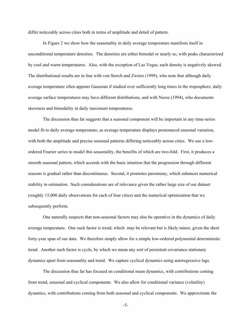
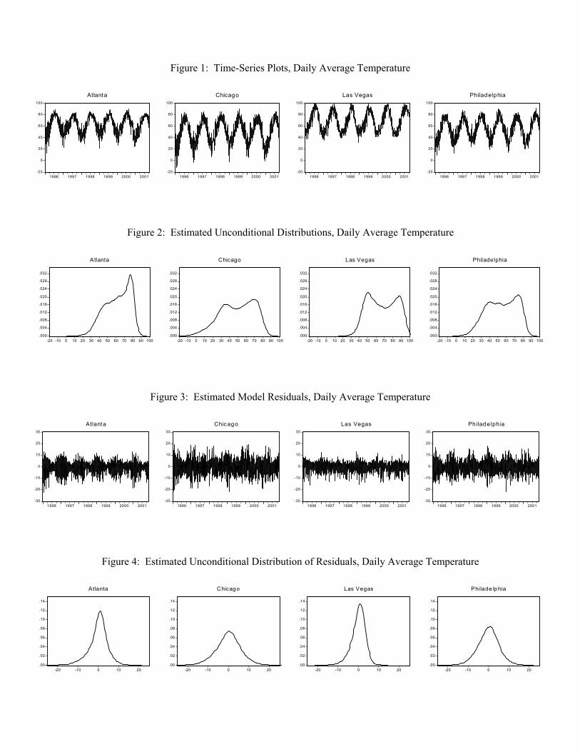
Before proceeding to detailed modeling and forecasting results, it is useful to get an overall feel for

the daily average temperature data. In Figure 1 we plot the daily average temperature series for the last five

years of the sample. The time-series plots reveal strong and unsurprising seasonality in average

temperature: in each city, the daily average temperature moves repeatedly and regularly through periods of

high temperature (summer) and low temperature (winter). Importantly, however, the seasonal fluctuations

-5-

differ noticeably across cities both in terms of amplitude and detail of pattern.

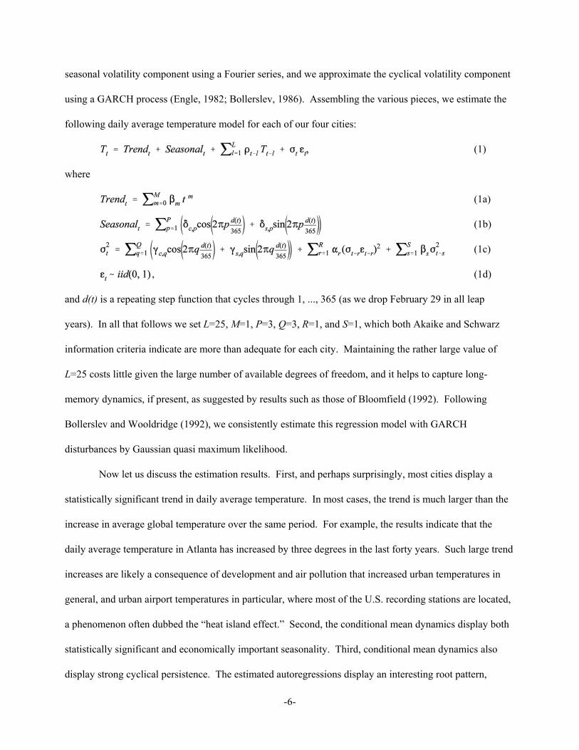
In Figure 2 we show how the seasonality in daily average temperature manifests itself in

unconditional temperature densities. The densities are either bimodal or nearly so, with peaks characterized

by cool and warm temperatures. Also, with the exception of Las Vegas, each density is negatively skewed.

The distributional results are in line with von Storch and Zwiers (1999), who note that although daily

average temperature often appears Gaussian if studied over sufficiently long times in the troposphere, daily

average surface temperatures may have different distributions, and with Neese (1994), who documents

skewness and bimodality in daily maximum temperatures.

The discussion thus far suggests that a seasonal component will be important in any time-series

model fit to daily average temperature, as average temperature displays pronounced seasonal variation,

with both the amplitude and precise seasonal patterns differing noticeably across cities. We use a low-

ordered Fourier series to model this seasonality, the benefits of which are two-fold. First, it produces a

smooth seasonal pattern, which accords with the basic intuition that the progression through different

seasons is gradual rather than discontinuous. Second, it promotes parsimony, which enhances numerical

stability in estimation. Such considerations are of relevance given the rather large size of our dataset

(roughly 15,000 daily observations for each of four cities) and the numerical optimization that we

subsequently perform.

One naturally suspects that non-seasonal factors may also be operative in the dynamics of daily

average temperature. One such factor is trend, which may be relevant but is likely minor, given the short

forty-year span of our data. We therefore simply allow for a simple low-ordered polynomial deterministic

trend. Another such factor is cycle, by which we mean any sort of persistent covariance stationary

dynamics apart from seasonality and trend. We capture cyclical dynamics using autoregressive lags.

The discussion thus far has focused on conditional mean dynamics, with contributions coming

from trend, seasonal and cyclical components. We also allow for conditional variance (volatility)

dynamics, with contributions coming from both seasonal and cyclical components. We approximate the

-6-

seasonal volatility component using a Fourier series, and we approximate the cyclical volatility component

using a GARCH process (Engle, 1982; Bollerslev, 1986). Assembling the various pieces, we estimate the

following daily average temperature model for each of our four cities:

(1)

where

(1a)

(1b)

(1c)

, (1d)

and d(t) is a repeating step function that cycles through 1, ..., 365 (as we drop February 29 in all leap

years). In all that follows we set L=25, M=1, P=3, Q=3, R=1, and S=1, which both Akaike and Schwarz

information criteria indicate are more than adequate for each city. Maintaining the rather large value of

L=25 costs little given the large number of available degrees of freedom, and it helps to capture long-

memory dynamics, if present, as suggested by results such as those of Bloomfield (1992). Following

Bollerslev and Wooldridge (1992), we consistently estimate this regression model with GARCH

disturbances by Gaussian quasi maximum likelihood.

Now let us discuss the estimation results. First, and perhaps surprisingly, most cities display a

statistically significant trend in daily average temperature. In most cases, the trend is much larger than the

increase in average global temperature over the same period. For example, the results indicate that the

daily average temperature in Atlanta has increased by three degrees in the last forty years. Such large trend

increases are likely a consequence of development and air pollution that increased urban temperatures in

general, and urban airport temperatures in particular, where most of the U.S. recording stations are located,

a phenomenon often dubbed the “heat island effect.” Second, the conditional mean dynamics display both

statistically significant and economically important seasonality. Third, conditional mean dynamics also

display strong cyclical persistence. The estimated autoregressions display an interesting root pattern,

-7-

common across all four cities, regardless of location. The dominant root is large and real, around 0.85, the

second and third roots are a conjugate pair with moderate modulus, around .3, and all subsequent roots are

much smaller in modulus. Fourth, the conditional variance dynamics, like the conditional mean dynamics

contain both seasonal (Fourier) and cyclical (GARCH) components. The Fourier terms appear to capture

adequately all volatility seasonality, and the GARCH terms capture the remaining “standard” volatility

persistence in daily average temperature. The Fourier volatility seasonality effect is relatively more

important; it is significant and sizeable for all cities. The GARCH volatility persistence effect is smaller,

although all cities have significant , ranging across cities between 0.01 and 0.07. There is considerably

more range in the estimates of volatility persistence as summarized by the other GARCH parameter, ,

implying very different half-lives of volatility shocks across cities. For example, the half-life of a Las

Vegas volatility shock is approximately one day, whereas the half-life of a Chicago volatility shock is

approximately seven days.

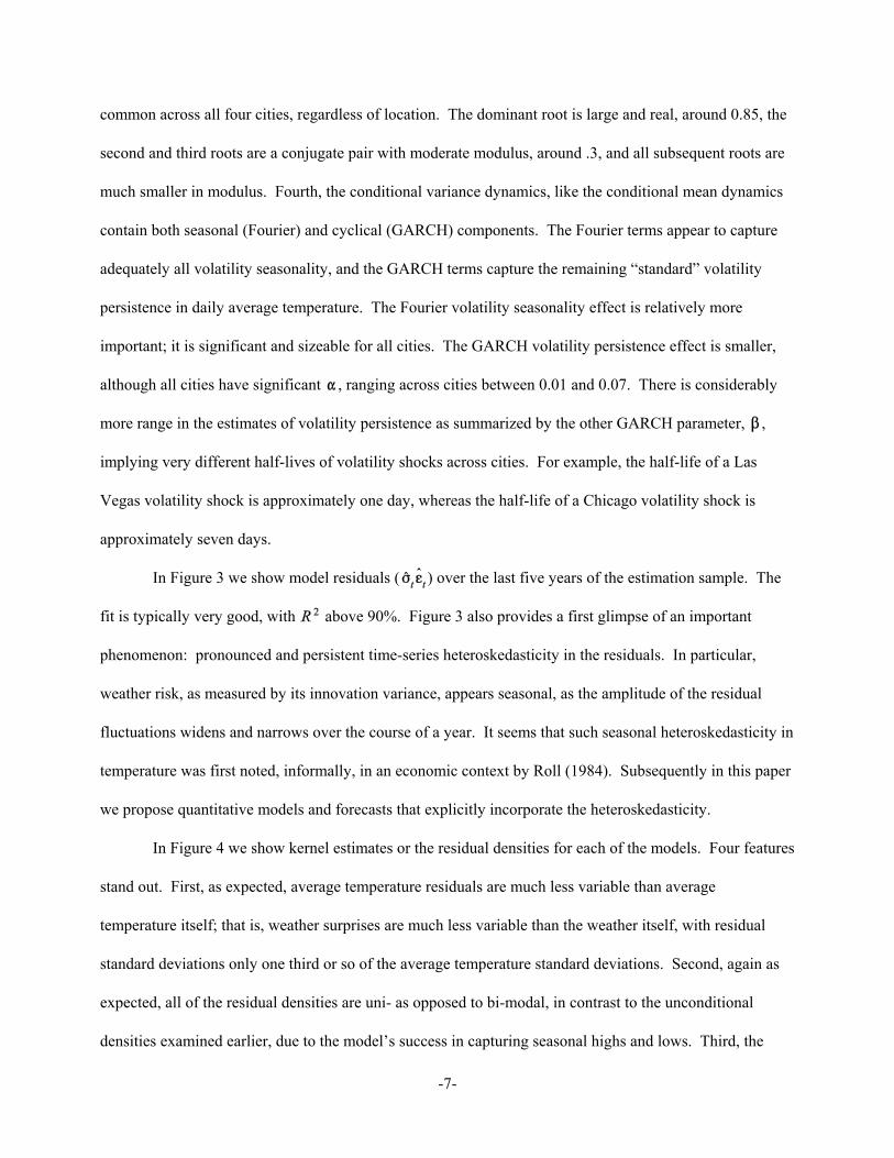
In Figure 3 we show model residuals ( ) over the last five years of the estimation sample. The

fit is typically very good, with above 90%. Figure 3 also provides a first glimpse of an important

phenomenon: pronounced and persistent time-series heteroskedasticity in the residuals. In particular,

weather risk, as measured by its innovation variance, appears seasonal, as the amplitude of the residual

fluctuations widens and narrows over the course of a year. It seems that such seasonal heteroskedasticity in

temperature was first noted, informally, in an economic context by Roll (1984). Subsequently in this paper

we propose quantitative models and forecasts that explicitly incorporate the heteroskedasticity.

In Figure 4 we show kernel estimates or the residual densities for each of the models. Four features

stand out. First, as expected, average temperature residuals are much less variable than average

temperature itself; that is, weather surprises are much less variable than the weather itself, with residual

standard deviations only one third or so of the average temperature standard deviations. Second, again as

expected, all of the residual densities are uni- as opposed to bi-modal, in contrast to the unconditional

densities examined earlier, due to the model’s success in capturing seasonal highs and lows. Third, the

-8-

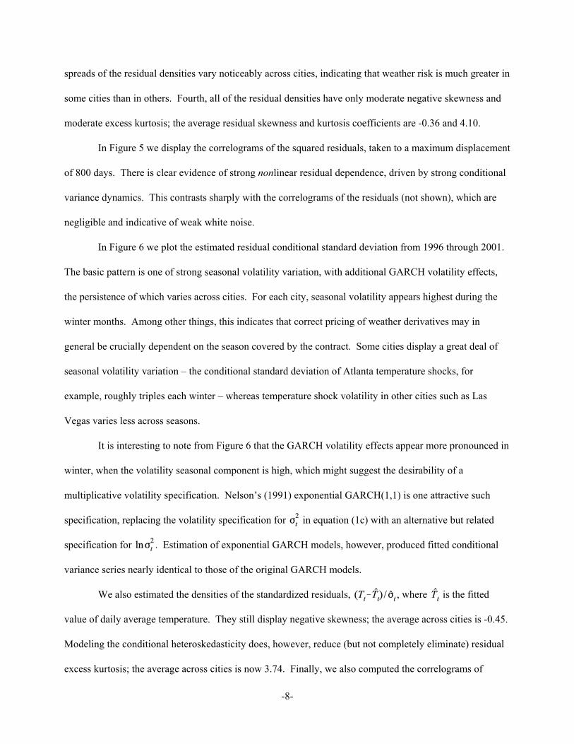
spreads of the residual densities vary noticeably across cities, indicating that weather risk is much greater in

some cities than in others. Fourth, all of the residual densities have only moderate negative skewness and

moderate excess kurtosis; the average residual skewness and kurtosis coefficients are -0.36 and 4.10.

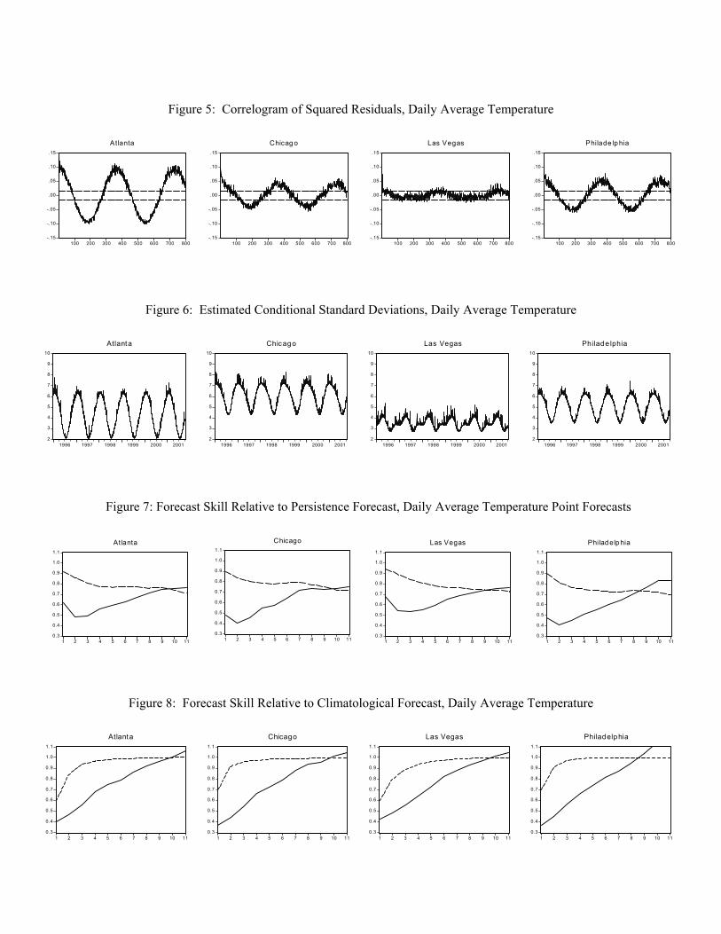
In Figure 5 we display the correlograms of the squared residuals, taken to a maximum displacement

of 800 days. There is clear evidence of strong nonlinear residual dependence, driven by strong conditional

variance dynamics. This contrasts sharply with the correlograms of the residuals (not shown), which are

negligible and indicative of weak white noise.

In Figure 6 we plot the estimated residual conditional standard deviation from 1996 through 2001.

The basic pattern is one of strong seasonal volatility variation, with additional GARCH volatility effects,

the persistence of which varies across cities. For each city, seasonal volatility appears highest during the

winter months. Among other things, this indicates that correct pricing of weather derivatives may in

general be crucially dependent on the season covered by the contract. Some cities display a great deal of

seasonal volatility variation – the conditional standard deviation of Atlanta temperature shocks, for

example, roughly triples each winter – whereas temperature shock volatility in other cities such as Las

Vegas varies less across seasons.

It is interesting to note from Figure 6 that the GARCH volatility effects appear more pronounced in

winter, when the volatility seasonal component is high, which might suggest the desirability of a

multiplicative volatility specification. Nelson’s (1991) exponential GARCH(1,1) is one attractive such

specification, replacing the volatility specification for in equation (1c) with an alternative but related

specification for . Estimation of exponential GARCH models, however, produced fitted conditional

variance series nearly identical to those of the original GARCH models.

We also estimated the densities of the standardized residuals, , where is the fitted

value of daily average temperature. They still display negative skewness; the average across cities is -0.45.

Modeling the conditional heteroskedasticity does, however, reduce (but not completely eliminate) residual

excess kurtosis; the average across cities is now 3.74. Finally, we also computed the correlograms of

-9-

squared standardized residuals; there is no significant deviation from white noise behavior, indicating that

the fitted model (1) is adequate.

3. Time-Series Weather Forecasting

Armed with a hopefully adequate time-series model for daily average temperature, we now proceed

to examine its performance in out-of-sample weather forecasting. We begin by examining its performance

in short-horizon point forecasting, despite the fact that short horizons and point forecasts are not of

maximal relevance for weather derivatives, in order to compare our performance to that of a very

sophisticated leading meteorological forecast. One naturally suspects that the much larger information set

on which the meteorological forecast is based will result in superior short-horizon point forecasting

performance, but even if so, of great interest is the question of how quickly and with what pattern the

superiority of the meteorological forecast deteriorates with forecast horizon.

We then progress to assess the performance of our model’s long-horizon density forecasts, which

are of maximal interest in weather derivative contexts, given the underlying option pricing considerations.

Simultaneously, we also move to forecasting rather than . This lets us match the most common

weather derivative “underlying,” and it also lets us explore the effects of using a daily model to produce

much longer-horizon density forecasts.

Point Forecasting

We assess the short-term accuracy of daily average temperature forecasts based on our

seasonal+trend+cycle model. In what follows, we refer to those forecasts as “autoregressive forecasts,” for

obvious reasons. We evaluate the autoregressive forecasts relative to three benchmark competitors, which

range from rather naive to very sophisticated. The first benchmark forecast is a no-change forecast. The

no-change forecast, often called the “persistence forecast” in the climatological literature, is the minimum

mean squared error forecast at all horizons if daily average temperature follows a random walk.

The second benchmark forecast is from a more sophisticated two-component (seasonal+trend)

model. It captures (daily) seasonal effects via day-of-year dummy variables, in keeping with the common

-10-

climatological use of daily averages as benchmarks, and it captures trend via a simple linear deterministic

function of time. We refer to this forecast as the “climatological forecast.”

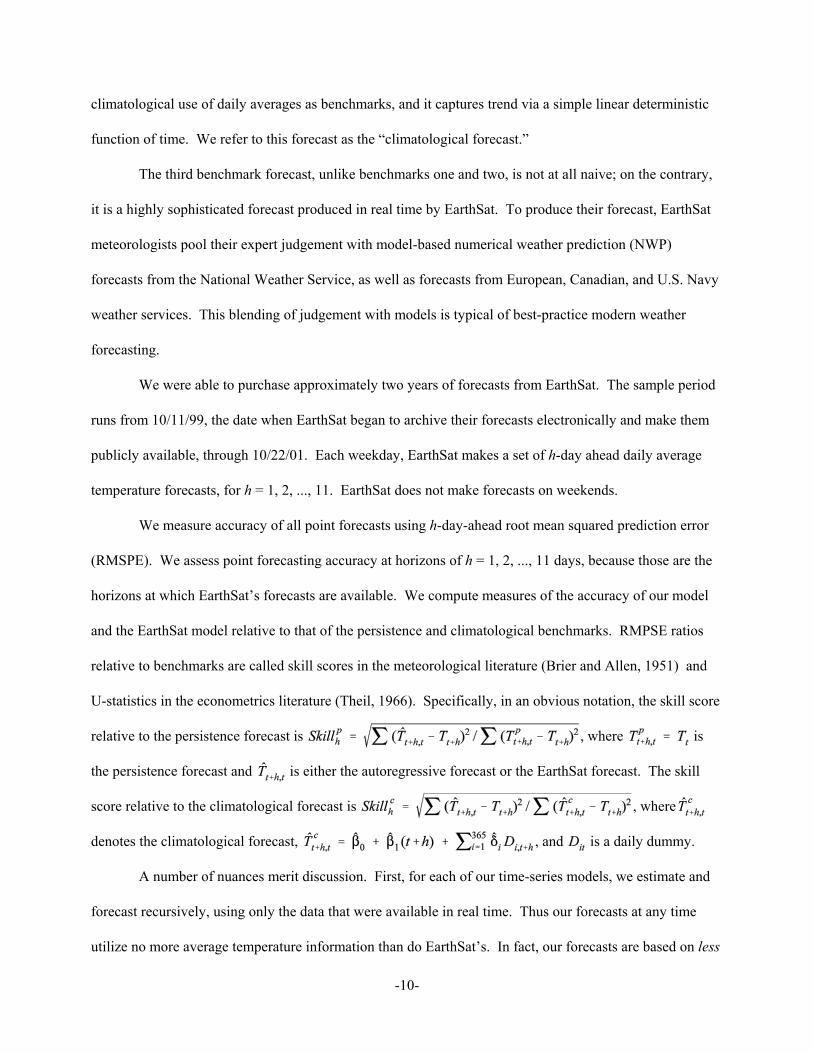
The third benchmark forecast, unlike benchmarks one and two, is not at all naive; on the contrary,

it is a highly sophisticated forecast produced in real time by EarthSat. To produce their forecast, EarthSat

meteorologists pool their expert judgement with model-based numerical weather prediction (NWP)

forecasts from the National Weather Service, as well as forecasts from European, Canadian, and U.S. Navy

weather services. This blending of judgement with models is typical of best-practice modern weather

forecasting.

We were able to purchase approximately two years of forecasts from EarthSat. The sample period

runs from 10/11/99, the date when EarthSat began to archive their forecasts electronically and make them

publicly available, through 10/22/01. Each weekday, EarthSat makes a set of h-day ahead daily average

temperature forecasts, for h = 1, 2, ..., 11. EarthSat does not make forecasts on weekends.

We measure accuracy of all point forecasts using h-day-ahead root mean squared prediction error

(RMSPE). We assess point forecasting accuracy at horizons of h = 1, 2, ..., 11 days, because those are the

horizons at which EarthSat’s forecasts are available. We compute measures of the accuracy of our model

and the EarthSat model relative to that of the persistence and climatological benchmarks. RMPSE ratios

relative to benchmarks are called skill scores in the meteorological literature (Brier and Allen, 1951) and

U-statistics in the econometrics literature (Theil, 1966). Specifically, in an obvious notation, the skill score

relative to the persistence forecast is , where is

the persistence forecast and is either the autoregressive forecast or the EarthSat forecast. The skill

score relative to the climatological forecast is , where

denotes the climatological forecast, , and is a daily dummy.

A number of nuances merit discussion. First, for each of our time-series models, we estimate and

forecast recursively, using only the data that were available in real time. Thus our forecasts at any time

utilize no more average temperature information than do EarthSat’s. In fact, our forecasts are based on less

-11-

average temperature information: our forecast for day t+1 made on day t is based on daily average

temperature through 11:59 PM of day t, whereas the EarthSat forecast for day t+1, which is not released

until 6:45 AM on day t+1, potentially makes use of the history of temperature through 6:45 AM of day

t+1. Second, we make forecasts using our models only on the dates that EarthSat made forecasts. In

particular, we make no forecasts on weekends. Hence, our accuracy comparisons proceed by averaging

squared errors over precisely the same days as those corresponding to the EarthSat errors. This ensures a

fair apples-to-apples comparison.

We report RMSPEs in Table 1 at horizons of h = 1, 3, 5, 7, 9, and 11 days, for all cities and

forecasting models. In addition, we graph skill scores as a function of horizon, against the persistence

forecast in Figure 7 and against the climatological forecast in Figure 8, for all cities and horizons. The

results are the same for all cities, so it is not necessary to discuss them individually by city. The results

most definitely do differ, however, across models and horizons, as we now discuss. We first discuss the

performance of the time-series forecasts, and then we discuss the EarthSat forecasts.

Let us consider first the forecasting performance of the persistence, climatological, and

autoregressive models across the various horizons. First consider the comparative performance of the

persistence and climatological forecasts. When h=1, the climatological forecasts are much worse than the

persistence forecasts, reflecting the fact that persistence in daily average temperature renders the

persistence forecast quite accurate at very short horizons. As the horizon lengthens, however, this result is

reversed: the persistence forecast becomes comparatively poor, as the temperature today has rather little to

do with the temperature, for example, nine days from now.

Second, consider the performance of the autoregressive forecasts relative to the persistence and

climatological forecasts. Even when h=1, the autoregressive forecasts consistently outperform the

persistence forecast, and their relative superiority increases with horizon. The autoregressive forecasts also

outperform the climatological forecasts at short horizons, but their comparative superiority decreases with

horizon. The performance of the autoregressive forecast is commensurate with that of the climatological

-12-

forecast roughly by the time h=4, indicating that the cyclical dynamics captured by the autoregressive

model via the inclusion of lagged dependent variables, which are responsible for its superior performance

at shorter horizons, are not very persistent and therefore not readily exploited for superior forecast

performance at longer horizons.

Now let us compare the forecasting performance of the autoregressive model and the EarthSat

model. When h=1, the EarthSat forecasts are much better than the autoregressive forecasts (which in turn

are better then either the persistence or climatological forecasts). Figures 7 and 8 make clear, however, that

the EarthSat forecasts outperform the autoregressive forecasts by progressively less as the horizon

lengthens, with nearly identical performance obtaining by the time h=8. One could even make a case that

the point forecasting performances of EarthSat and our three-component model become indistinguishable

before h=8 (say, by h=5) if one were to account for the sampling error in the estimated RMSPEs and for the

fact that the EarthSat information set for any day t actually contains a few hours of the next day.

All told, we view our model’s point forecasting performance as neither particularly encouraging

nor particularly discouraging, at the longer horizons of relevance for weather derivatives (one to six

months, say). Its point forecasting performance is not particularly encouraging: although it appears no

worse than its competitors, it also appears no better. But its point forecasting performance is also not

particularly discouraging: the nature of temperature dynamics simply makes temperature very difficult to

forecast at long horizons, whether by our method or any other, as all point forecasts revert fairly quickly to

the climatological forecast, and hence all long-horizon forecasts are “equally poor.”

It is crucial to recognize, however, that a key object in any statistical analysis involving weather

derivatives, and indeed the key object for the central issue weather derivative pricing, is the entire

conditional density of the future weather outcome. The point forecast is the conditional mean, which

describes just one feature of that conditional density, namely its location. Hence the fact that the long-

horizon conditional mean estimate produced by our model is no better that produced by the climatological

model does not imply that our model or framework fails to deliver value-added. On the contrary, a great

-13-

virtue of our approach is its immediate and simple generalization to provide entire density forecasts. The

key feature of daily average temperature conditional density dynamics, apart from the seasonal conditional

mean dynamics, is the highly seasonal conditional variance dynamics, which we have modeled

parsimoniously and successfully. This facilitates simple modeling of time-varying scale of the conditional

density, and it is as relevant for long horizons as for short. All of this adds up to a simple yet powerful

framework for producing density forecasts of weather variables, to which we now turn. It is telling to

observe that in what follows we must evaluate the performance of our density forecasts in absolute terms,

rather than relative to EarthSat density forecasts, because EarthSat, like almost all forecasters, does not

even produce density forecasts.

Density Forecasting

In this section, we shift our focus to long-horizon density forecasting, and to cumulative heating

degree days, all of which is of crucial relevance for weather derivatives. Heating degree days for day t is

simply . We use our model of daily average temperature to produce density

forecasts of cumulative HDDs from November 1 through March 31, for each city and for each year

between 1960 and 2000, defined as for y = 1960, ..., 2000, i = 1, ..., 4.

Because we remove February 29 from each leap year, each sum contains exactly 151 days. We use full-

sample as opposed to recursive parameter estimates, as required by the very small number of CumHDD

observations. To avoid unnecessarily burdensome notation, we will often drop the y and i subscripts when

the meaning is clear from context.

We focus on CumHDD for two important reasons. First, weather derivative contracts are often

written on the cumulative sum of a weather related outcome over a fixed horizon, as with the cumulative

HDD and CDD contracts traded on the CME. Second, and related, the November-March HDD contract is

one of the most actively traded weather-related contracts and hence is of substantial direct interest.

On October 31 of each year, and for each city, we use the estimated daily model to produce a

density forecast of CumHDD for the following winter’s heating season. We simulate 250 realizations of

-14-

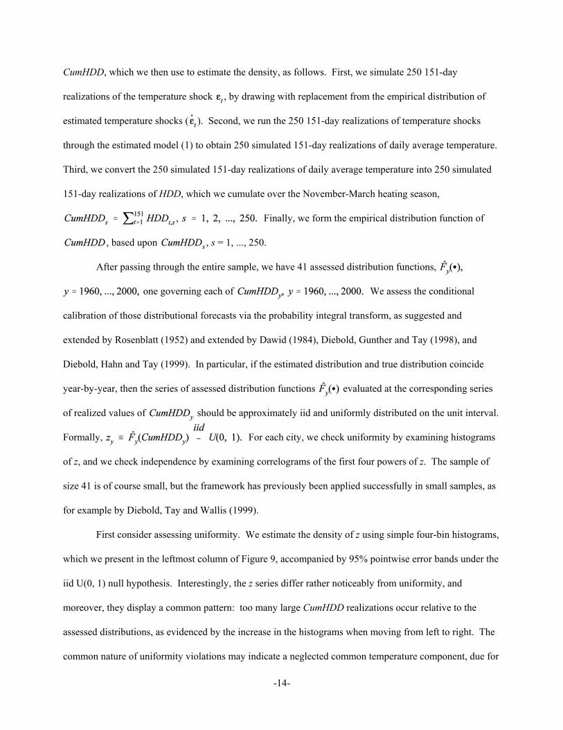
CumHDD, which we then use to estimate the density, as follows. First, we simulate 250 151-day

realizations of the temperature shock , by drawing with replacement from the empirical distribution of

estimated temperature shocks ( ). Second, we run the 250 151-day realizations of temperature shocks

through the estimated model (1) to obtain 250 simulated 151-day realizations of daily average temperature.

Third, we convert the 250 simulated 151-day realizations of daily average temperature into 250 simulated

151-day realizations of HDD, which we cumulate over the November-March heating season,

, Finally, we form the empirical distribution function of

, based upon , s = 1, ..., 250.

After passing through the entire sample, we have 41 assessed distribution functions,

one governing each of We assess the conditional

calibration of those distributional forecasts via the probability integral transform, as suggested and

extended by Rosenblatt (1952) and extended by Dawid (1984), Diebold, Gunther and Tay (1998), and

Diebold, Hahn and Tay (1999). In particular, if the estimated distribution and true distribution coincide

year-by-year, then the series of assessed distribution functions evaluated at the corresponding series

of realized values of should be approximately iid and uniformly distributed on the unit interval.

Formally, For each city, we check uniformity by examining histograms

of z, and we check independence by examining correlograms of the first four powers of z. The sample of

size 41 is of course small, but the framework has previously been applied successfully in small samples, as

for example by Diebold, Tay and Wallis (1999).

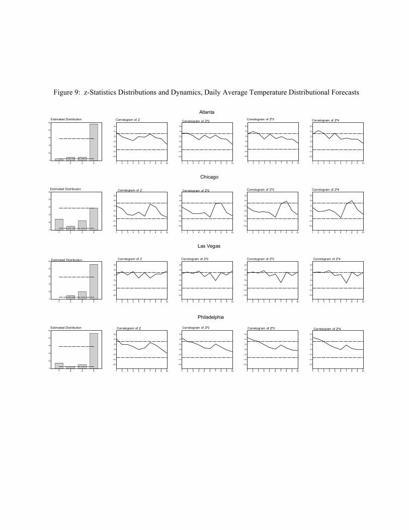
First consider assessing uniformity. We estimate the density of z using simple four-bin histograms,

which we present in the leftmost column of Figure 9, accompanied by 95% pointwise error bands under the

iid U(0, 1) null hypothesis. Interestingly, the z series differ rather noticeably from uniformity, and

moreover, they display a common pattern: too many large CumHDD realizations occur relative to the

assessed distributions, as evidenced by the increase in the histograms when moving from left to right. The

common nature of uniformity violations may indicate a neglected common temperature component, due for

-15-

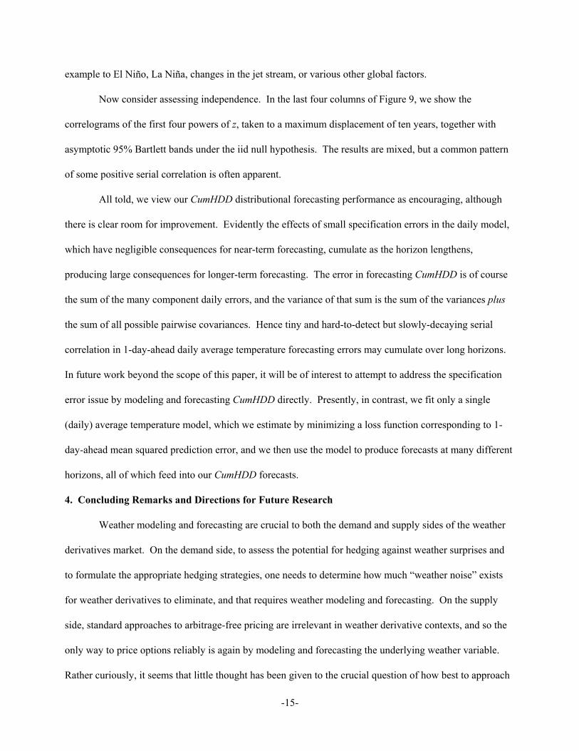
example to El Niño, La Niña, changes in the jet stream, or various other global factors.

Now consider assessing independence. In the last four columns of Figure 9, we show the

correlograms of the first four powers of z, taken to a maximum displacement of ten years, together with

asymptotic 95% Bartlett bands under the iid null hypothesis. The results are mixed, but a common pattern

of some positive serial correlation is often apparent.

All told, we view our CumHDD distributional forecasting performance as encouraging, although

there is clear room for improvement. Evidently the effects of small specification errors in the daily model,

which have negligible consequences for near-term forecasting, cumulate as the horizon lengthens,

producing large consequences for longer-term forecasting. The error in forecasting CumHDD is of course

the sum of the many component daily errors, and the variance of that sum is the sum of the variances plus

the sum of all possible pairwise covariances. Hence tiny and hard-to-detect but slowly-decaying serial

correlation in 1-day-ahead daily average temperature forecasting errors may cumulate over long horizons.

In future work beyond the scope of this paper, it will be of interest to attempt to address the specification

error issue by modeling and forecasting CumHDD directly. Presently, in contrast, we fit only a single

(daily) average temperature model, which we estimate by minimizing a loss function corresponding to 1-

day-ahead mean squared prediction error, and we then use the model to produce forecasts at many different

horizons, all of which feed into our CumHDD forecasts.

4. Concluding Remarks and Directions for Future Research

Weather modeling and forecasting are crucial to both the demand and supply sides of the weather

derivatives market. On the demand side, to assess the potential for hedging against weather surprises and

to formulate the appropriate hedging strategies, one needs to determine how much “weather noise” exists

for weather derivatives to eliminate, and that requires weather modeling and forecasting. On the supply

side, standard approaches to arbitrage-free pricing are irrelevant in weather derivative contexts, and so the

only way to price options reliably is again by modeling and forecasting the underlying weather variable.

Rather curiously, it seems that little thought has been given to the crucial question of how best to approach

-16-

weather modeling and forecasting in the context of weather derivative demand and supply. The vast

majority of extant weather forecasting literature has a structural “atmospheric science” feel, and although

such an approach is surely best for forecasting at very short horizons, as verified both by our own results

and those of numerous others, it is not obvious that it is best for the longer horizons relevant for weather

derivatives, such as twelve weeks or six months. Moreover, it is distributional forecasts, not point

forecasts, that are of maximal relevance in the derivatives context. Good distributional forecasting does not

necessarily require a structural model, but it does require accurate approximations to stochastic dynamics.

In this paper we took an arguably-naive nonstructural time-series approach to modeling and

forecasting daily average temperature in four U.S. cities, and we inquired systematically as to whether it

proves useful. The answer, perhaps surprisingly, was a qualified yes. Our point forecasts were always at

least as good as the persistence and climatological forecasts, but were still not as good as the

judgementally-adjusted NWP forecast produced by EarthSat until a horizon of eight days, after which all

point forecasts performed equally well. Crucially, we also documented and modeled the strong seasonality

in weather surprise volatility, and we assessed the adequacy of long-horizon distributional forecasts that

accounted for it, with mixed but encouraging results. We found, moreover, an interesting commonality in

the patterns of cross-city deviations from perfect conditional calibration, indicating possible dependence on

common latent components, perhaps due to El Niño or La Niña.

All told, we would assert that in the context of weather modeling as relevant for weather

derivatives, it appears that simple yet sophisticated time-series models and forecasts perform at least well

enough to suggest the desirability of additional exploration. When, in addition, one considers that time-

series models and methods are inexpensive, easily replicated, easily extended, beneficially intrinsically

stochastic, and capable of producing both point and density forecasts at a variety of horizons, we believe

that a strong case exists for their use in the context of modeling and forecasting as relevant for weather

derivatives.

We would also assert that our views are consistent with the mainstream consensus in atmospheric

-17-

science. In his well-known text, for example, Wilks (1995, p. 159) notes that “[Statistical weather

forecasting] methods are still viable and useful at very short lead times (hours in advance) or very long lead

times (weeks or more in advance) for which NWP information is either not available with sufficient

promptness or accuracy, respectively.” Indeed, in many respects our results are simply an extensive

confirmation of Wilks’ assertion in the context of weather derivatives, which are of great current interest.

Ultimately, our present view on weather forecasting for weather derivatives is that climatological

forecasts are what we need, but that standard point climatological forecasts – effectively little more than

daily averages – are much too restrictive. Instead, we seek “generalized climatological forecasts” from

richer models tracking entire conditional distributions, and modern time-series statistical methods may have

much to contribute. We view the present paper as a “call to action,” with our simple model representing a

step toward a fully generalized climatological forecast, but with many important issues remaining

unexplored. Here we briefly discuss a few that we find particularly intriguing.

One of the contributions of this paper is our precise quantification of daily average temperature

conditional variance dynamics. But richer dynamics might be beneficially permitted in both lower-ordered

conditional moments (the conditional mean) and higher-ordered conditional moments (such as the

conditional skewness and kurtosis). As regards the conditional mean, one could introduce explanatory

variables, as in Visser and Molenaar (1995), who condition on a volcanic activity index, sunspot numbers,

and a southern oscillation index. Relevant work also includes Jones (1996) and Pozo et al. (1998), but

those papers use annual data and therefore miss the seasonal patterns in both conditional mean and

conditional variance dynamics so crucial for weather derivatives demand and supply. One could also allow

for nonlinear effects, most notably stochastic regime switching, which might aid, for example, in the

detection of El Niño and La Niña events. (See Richman and Montroy, 1996, and also Zwiers and von

Storch, 1990.) As regards the conditional skewness and kurtosis, one could model them directly, as for

example with the autoregressive conditional skewness model of Harvey and Siddique (1999).

Alternatively, one could directly model the evolution of the entire conditional density, as in Hansen (1994).

-18-

Aspects of multivariate analysis and cross-hedging also hold promise for future work. Cross-city

correlations may be crucially important, because they govern the potential for cross-hedging. Hedging

weather risk in a remote Midwestern location might, for example, be prohibitively expensive or even

impossible due to illiquid or nonexistent markets, but if that risk is highly correlated with Chicago’s

weather risk, for which a liquid market exists, effective hedging may still be possible. Hence an obvious

and important extension of the univariate temperature analysis reported in the present paper is multivariate

modeling of daily average temperature in a set of cities, allowing for a time-varying innovation variance-

covariance matrix. Of particular interest would be the fitted and forecasted conditional mean, conditional

variance and conditional covariance dynamics, the covariance matrices of standardized innovations, and the

impulse response functions (which chart the speed and pattern with which weather surprises in one location

are transmitted to other locations).

Another interesting multivariate issue involves weather-related swings in earnings and share prices.

It will be of interest to use the size of weather-related swings in earnings as way to assess the potential for

weather derivatives use. In particular, we need to understand how weather surprises translate into earnings

surprises, which then translate into stock return movements. Some interesting subtleties may arise. As one

example, note that only systematic weather risk should be priced, which raises the issue of how to

disentangle systematic and non-systematic weather risks. As a second example, note that there may be

nonlinearities in the relationship between prices and the weather induced via path dependence; if there is an

early freeze, for example, then it doesn’t matter how good the weather is subsequently: the crop will be

ruined and prices will be high (see Richardson, Bodoukh, Sjen, and Whitelaw, 2001).

References

Black, F. and Scholes, M. (1973), The Pricing of Options and Corporate Liabilities,” Journal of Political

Economy, 81, 637-654.

Bloomfield, P. (1992), “Trends in Global Temperature,” Climate Change, 21, 1-16.

-19-

Bollerslev, T. and Wooldridge, J.M. (1992), “Quasi-Maximum Likelihood Estimation and Inference in

Dynamic Models with Time Varying Covariances,” Econometric Reviews, 11, 143-172.

Brier, G.W. and Allen, R.A. (1951), “Verification of Weather Forecasts,” in T.F. Malone (ed.),

Compendium of Meteorology, American Meteorological Society.

Campbell, S.D. and Diebold, F.X. (2002), “Weather Forecasting for Weather Derivatives (first version),”

Working Paper No. 02-42, Wharton Financial Institutions Center.

Campbell, S.D. and Diebold, F.X. (2003), “Weather Forecasting for Weather Derivatives (second

version),” Working Paper No. 10141, National Bureau of Economic Research.

Cao, M. and Wei, J. (2001), “Pricing Weather Derivatives: An Equilibrium Approach,” Manuscript,

University of York and University of Toronto.

Davis, M. (2001), “Pricing Weather Derivatives by Marginal Value,” Quantitative Finance, 1, 305-308.

Dawid, A.P. (1984), “Statistical Theory: The Prequential Approach,” Journal of the Royal Statistical

Society, Series A, 147, 278-292.

Diebold, F.X. (2004), Elements of Forecasting, Third Edition. Cincinnati: South-Western.

Diebold, F.X., Gunther, T. and Tay, A.S. (1998), “Evaluating Density Forecasts, with Applications to

Financial Risk Management,” International Economic Review, 39, 863-883.

Diebold, F.X., Hahn, J. and Tay, A.S. (1999), “Multivariate Density Forecast Evaluation and Calibration in

Financial Risk Management: High-Frequency Returns on Foreign Exchange,” Review of

Economics and Statistics, 81, 661-673.

Diebold, F.X., Tay, A.S. and Wallis, K. (1999), “Evaluating Density Forecasts of Inflation: The Survey of

Professional Forecasters,” in R. Engle and H. White (eds.), Cointegration, Causality, and

Forecasting: A Festschrift in Honor of Clive W.J. Granger, 76-90, Oxford University Press.

Dischel, R.S., ed. (2002), Climate Risk and the Weather Market: Financial Risk Management with

Weather Hedges. London: Risk Publications.

Engle, R.F. (1982), “Autoregressive Conditional Heteroskedasticity with Estimates of the Variance of U.K.

-20-

Inflation,” Econometrica, 50, 987-1008.

Geman, H., Ed. (1999), Insurance and Weather Derivatives: From Exotic Options to Exotic Underlyings.

London: Risk Publications.

Hansen, B.E. (1994), “Autoregressive Conditional Density Estimation,” International Economic Review,

35, 705-730.

Harvey, A.C. (1989), Forecasting, Structural Time Series Models and the Kalman Filter. Cambridge:

Cambridge University Press.

Harvey, C.R. and Siddique, A. (1999), “Autoregressive Conditional Skewness,” Journal of Financial and

Quantitative Analysis, 34, 465-488.

Hyndman, R.J. and Grunwald, G.K. (2000), “Generalized Additive Modeling of Mixed Distribution

Markov Models with Application to Melbourne's Rainfall,” Australian and New Zealand Journal

of Statistics, 42, 145-158.

Jones, R.H. (1996), “The Potential of State Space Models in Statistical Meteorology,” Proceedings of the

13th Conference on Probability and Statistics in the Atmospheric Sciences, American

Meteorological Society.

Milionis, A.E. and Davies, T.D. (1994), “Box-Jenkins univariate Modeling for Climatological Time Series

Analysis: An Application to the Monthly Activity of Temperature Inversions,” International

Journal of Climatology, 14 569-579.

Neese, J.M. (1994), “Systematic Biases in Manual Observations of Maximum and Minimum Temperature,”

Journal of Climate, 7, 834-842.

Nelson, D.B. (1991), "Conditional Heteroskedasticity in Asset Returns: A New Approach," Econometrica,

59, 347-370.

Pozo, D., Esteban-Parra, M.J., Rodrigo, F.S. and Castro-Diez, Y. (1998), “ARIMA Structural Models for

Temperature Time Series of Spain,” Proceedings of the 14th Conference on Probability and

Statistics in the Atmospheric Sciences, American Meteorological Society.

-21-

Richardson, M., Bodoukh, J., Sjen, Y. and Whitelaw, R. (2001), “Freshly Squeezed: A Reinterpretation of

Market Rationality in the Orange Juice Futures Market,” Working Paper, New York University.

Richman, M.B. and Montroy, D.L. (1996), “Nonlinearities in the Signal Between El Niño / La Niña Events

and North American Precipitation and Temperature,” Proceedings of the 13th Conference on

Probability and Statistics in the Atmospheric Sciences, American Meteorological Society.

Roll, R. (1984), “Orange Juice and Weather,” American Economic Review, 74, 861-880.

Rosenblatt, M. (1952), “Remarks on a Multivariate Transformation,” Annals of Mathematical Statistics, 23,

470-472.

Seater, J.J. (1993), “World Temperature-Trend Uncertainties and Their Implications for Economic Policy,”

Journal of Business and Economic Statistics, 11, 265-277.

Storch, H. von and Zwiers, F.W. (1999), Statistical Analysis in Climate Research. Cambridge: Cambridge

University Press.

Theil, H. (1966), Applied Economic Forecasting. Amsterdam: North-Holland.

Torro, H., Meneu, V. and Valor E. (2001), “Single Factor Stochastic Models with Seasonality Applied to

Underlying Weather Derivatives Variables,” Manuscript, University of Valencia.

Tribia, J.J. (1997), “Weather Prediction,” in R. Katz and A. Murphy (eds.), Economic Value of Weather and

Climate Forecasts. Cambridge: Cambridge University Press.

Visser, H. and Molenaar, J. (1995), “Trend Estimation and Regression Analysis in Climatological Time

Series: An Application of Structural Time Series Models and the Kalman Filter,” Journal of

Climate, 8, 969-979.

Weather Risk (1998), Supplement to Risk Magazine, October.

Weather Risk (2000), Supplement to Risk Magazine, August.

Wilks, D.S. (1995), Statistical Methods in the Atmospheric Sciences. New York: Academic Press.

Zwiers, F.W. and von Storch, H. (1990), “Regime Dependent Autoregressive Time Series Modeling of the

Southern Oscillation,” Journal of Climate, 3, 1347-1363.

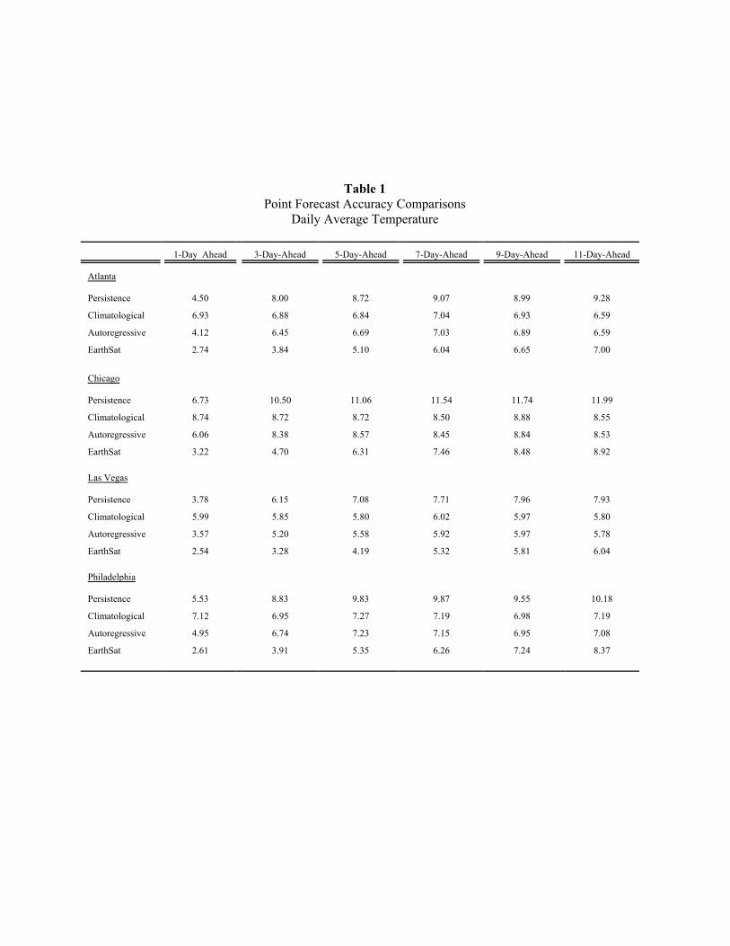
Table 1Point Forecast Accuracy Comparisons

Daily Average Temperature

1-Day Ahead 3-Day-Ahead 5-Day-Ahead 7-Day-Ahead 9-Day-Ahead 11-Day-Ahead

Atlanta

Persistence 4.50 8.00 8.72 9.07 8.99 9.28

Climatological 6.93 6.88 6.84 7.04 6.93 6.59

Autoregressive 4.12 6.45 6.69 7.03 6.89 6.59

EarthSat 2.74 3.84 5.10 6.04 6.65 7.00

Chicago

Persistence 6.73 10.50 11.06 11.54 11.74 11.99

Climatological 8.74 8.72 8.72 8.50 8.88 8.55

Autoregressive 6.06 8.38 8.57 8.45 8.84 8.53

EarthSat 3.22 4.70 6.31 7.46 8.48 8.92

Las Vegas

Persistence 3.78 6.15 7.08 7.71 7.96 7.93

Climatological 5.99 5.85 5.80 6.02 5.97 5.80

Autoregressive 3.57 5.20 5.58 5.92 5.97 5.78

EarthSat 2.54 3.28 4.19 5.32 5.81 6.04

Philadelphia

Persistence 5.53 8.83 9.83 9.87 9.55 10.18

Climatological 7.12 6.95 7.27 7.19 6.98 7.19

Autoregressive 4.95 6.74 7.23 7.15 6.95 7.08

EarthSat 2.61 3.91 5.35 6.26 7.24 8.37

.00

.02

.04

.06

.08

.10

.12

.14

-20 -10 0 10 20

Atlanta

.00

.02

.04

.06

.08

.10

.12

.14

-20 -10 0 10 20

Chicag o

.00

.02

.04

.06

.08

.10

.12

.14

-20 -10 0 10 20

Las Vegas

.00

.02

.04

.06

.08

.10

.12

.14

-20 -10 0 10 20

Philade lp hia

Figure 4: Estimated Unconditional Distribution of Residuals, Daily Average Temperature

-30

-20

-10

0

10

20

30

1996 1997 1998 1999 2000 2001

Atlanta

-30

-20

-10

0

10

20

30

1996 1997 1998 1999 2000 2001

Chicago

-30

-20

-10

0

10

20

30

1996 1997 1998 1999 2000 2001

Las Vegas

-30

-20

-10

0

10

20

30

1996 1997 1998 1999 2000 2001

Philad e lphia

Figure 3: Estimated Model Residuals, Daily Average Temperature

.000

.004

.008

.012

.016

.020

.024

.028

.032

-20 -10 0 10 20 30 40 50 60 70 80 90 100

Atlanta

.000

.004

.008

.012

.016

.020

.024

.028

.032

-20 -10 0 10 20 30 40 50 60 70 80 90 100

Chicago

.000

.004

.008

.012

.016

.020

.024

.028

.032

-20 -10 0 10 20 30 40 50 60 70 80 90 100

Las Vegas

.000

.004

.008

.012

.016

.020

.024

.028

.032

-20 -10 0 10 20 30 40 50 60 70 80 90 100

Philadelphia

Figure 2: Estimated Unconditional Distributions, Daily Average Temperature

-20

0

20

40

60

80

100

1996 1997 1998 1999 2000 2001

Atlanta

-20

0

20

40

60

80

100

1996 1997 1998 1999 2000 2001

Chicago

-20

0

20

40

60

80

100

1996 1997 1998 1999 2000 2001

Las Vegas

-20

0

20

40

60

80

100

1996 1997 1998 1999 2000 2001

Philadelphia

Figure 1: Time-Series Plots, Daily Average Temperature

0.3

0.4

0.5

0.6

0.7

0.8

0.9

1.0

1.1

1 2 3 4 5 6 7 8 9 10 11

Atlanta

0.3

0.4

0.5

0.6

0.7

0.8

0.9

1.0

1.1

1 2 3 4 5 6 7 8 9 10 11

Chicago

0.3

0.4

0.5

0.6

0.7

0.8

0.9

1.0

1.1

1 2 3 4 5 6 7 8 9 10 11

Las Vegas

0.3

0.4

0.5

0.6

0.7

0.8

0.9

1.0

1.1

1 2 3 4 5 6 7 8 9 10 11

Philadelphia

Figure 8: Forecast Skill Relative to Climatological Forecast, Daily Average Temperature

0.3

0.4

0.5

0.6

0.7

0.8

0.9

1.0

1.1

1 2 3 4 5 6 7 8 9 10 11

Atlanta

0.3

0.4

0.5

0.6

0.7

0.8

0.9

1.0

1.1

1 2 3 4 5 6 7 8 9 10 11

Chicago

0.3

0.4

0.5

0.6

0.7

0.8

0.9

1.0

1.1

1 2 3 4 5 6 7 8 9 10 11

Las Vegas

0.3

0.4

0.5

0.6

0.7

0.8

0.9

1.0

1.1

1 2 3 4 5 6 7 8 9 10 11

Philad elp hia

Figure 7: Forecast Skill Relative to Persistence Forecast, Daily Average Temperature Point Forecasts

2

3

4

5

6

7

8

9

10

1996 1997 1998 1999 2000 2001

Atlanta

2

3

4

5

6

7

8

9

10

1996 1997 1998 1999 2000 2001

Chicago

2

3

4

5

6

7

8

9

10

1996 1997 1998 1999 2000 2001

Las Vegas

2

3

4

5

6

7

8

9

10

1996 1997 1998 1999 2000 2001

Philad e lphia

Figure 6: Estimated Conditional Standard Deviations, Daily Average Temperature

-.15

-.10

-.05

.00

.05

.10

.15

100 200 300 400 500 600 700 800

Atlanta

-.15

-.10

-.05

.00

.05

.10

.15

100 200 300 400 500 600 700 800

Chicag o

-.15

-.10

-.05

.00

.05

.10

.15

100 200 300 400 500 600 700 800

Las Vegas

-.15

-.10

-.05

.00

.05

.10

.15

100 200 300 400 500 600 700 800

Philade lp hia

Figure 5: Correlogram of Squared Residuals, Daily Average Temperature

.1

.2

.3

.4

.5

.6

1 2 3 4

-.6

-.4

-.2

.0

.2

.4

.6

1 2 3 4 5 6 7 8 9 10

-.6

-.4

-.2

.0

.2

.4

.6

1 2 3 4 5 6 7 8 9 10

-.6

-.4

-.2

.0

.2

.4

.6

1 2 3 4 5 6 7 8 9 10

-.6

-.4

-.2

.0

.2

.4

.6

1 2 3 4 5 6 7 8 9 10

.1

.2

.3

.4

.5

.6

1 2 3 4

-.6

-.4

-.2

.0

.2

.4

.6

1 2 3 4 5 6 7 8 9 10

-.6

-.4

-.2

.0

.2

.4

.6

1 2 3 4 5 6 7 8 9 10

-.6

-.4

-.2

.0

.2

.4

.6

1 2 3 4 5 6 7 8 9 10

-.6

-.4

-.2

.0

.2

.4

.6

1 2 3 4 5 6 7 8 9 10

.1

.2

.3

.4

.5

.6

1 2 3 4

-.6

-.4

-.2

.0

.2

.4

.6

1 2 3 4 5 6 7 8 9 10

-.6

-.4

-.2

.0

.2

.4

.6

1 2 3 4 5 6 7 8 9 10

-.6

-.4

-.2

.0

.2

.4

.6

1 2 3 4 5 6 7 8 9 10

-.6

-.4

-.2

.0

.2

.4

.6

1 2 3 4 5 6 7 8 9 10

.1

.2

.3

.4

.5

.6

1 2 3 4

-.6

-.4

-.2

.0

.2

.4

.6

1 2 3 4 5 6 7 8 9 10

-.6

-.4

-.2

.0

.2

.4

.6

1 2 3 4 5 6 7 8 9 10

-.6

-.4

-.2

.0

.2

.4

.6

1 2 3 4 5 6 7 8 9 10

-.6

-.4

-.2

.0

.2

.4

.6

1 2 3 4 5 6 7 8 9 10

Atlanta

Chicago

Las Vegas

Philadelphia

Estimated Distribution Correlogram of Z Correlogram of Z^2 Correlogram of Z^3 Correlogram of Z^4

Estimated Distribution

Estimated Distribution

Estimated Distribution

Correlogram of Z Correlogram of Z^2 Correlogram of Z^3 Correlogram of Z^4

Correlogram of Z

Correlogram of Z

Correlogram of Z^2

Correlogram of Z^2

Correlogram of Z^3

Correlogram of Z^3

Correlogram of Z^4

Correlogram of Z^4

Figure 9: z-Statistics Distributions and Dynamics, Daily Average Temperature Distributional Forecasts

Notes to Tables and Figures

Table 1: We show each forecast’s root mean squared error, measured in degrees Fahrenheit.

Figure 1: Each panel displays a time-series plot of daily average temperature, 1996-2001.

Figure 2: Each panel displays a kernel density estimate of the unconditional distribution of daily average

temperature, 1960-2001. In each case, we employ the Epanechnikov kernel and select the bandwidth using

Silverman’s rule, .

Figure 3: Each panel displays the residuals from an unobserved-components model,

, 1996-2001.

Figure 4: Each panel displays a kernel density estimate of the distribution of the residuals from our daily

average temperature model, . In each case, we employ the

Epanechnikov kernel and select the bandwidth using Silverman’s rule, .

Figure 5: Each panel displays sample autocorrelations of the squared residuals from our daily average

temperature model, , together with Bartlett’s approximate ninety-

five percent confidence intervals under the null hypothesis of white noise.

Figure 6: Each panel displays a time series of estimated conditional standard deviations ( ) of daily

average temperature, where , 1996-2001.

Figure 7: Each panel displays the ratio of a forecast’s RMSPE to that of a persistence forecast, for 1-day-

ahead through 11-day-ahead horizons. The solid line refers to the EarthSat forecast, and the dashed line

refers to the autoregressive forecast. The forecast evaluation period is 10/11/99 - 10/22/01.

Figure 8: Each panel displays the ratio of a forecast’s RMSPE to that of a climatological forecast, for 1-

day-ahead through 11-day-ahead horizons. The solid line refers to the EarthSat forecast, and the dashed

line refers to the autoregressive forecast. The forecast evaluation period is 10/11/99 - 10/22/01.

Figure 9: Each row displays a histogram for z and correlograms for four powers of z, the probability

integral transform of cumulative November-March HDDs, 1960-2000. Dashed lines indicate approximate

ninety-five percent confidence intervals in the iid U(0,1) case of correct conditional calibration.

CFS Working Paper Series:

No. Author(s) Title

2003/48 Martin D. Dietz Screening and Advising by a Venture Capitalist with a Time Constraint

2004/01 Ivica Dus Raimond Maurer Olivia S. Mitchell

Betting on Death and Capital Markets in Retirement: A Shortfall Risk Analysis of Life Annuities versus Phased Withdrawal Plans

2004/02 Tereza Tykvová Uwe Walz

Are IPOs of Different VCs Different?

2004/03 Marc Escrihuela-Villar Innovation and Market Concentration with Asymmetric Firms

2004/04 Ester Faia Tommaso Monacelli

Ramsey Monetary Policy and International Relative Prices

2004/05 Uwe Wals Douglas Cumming

Private Equity Returns and Disclosure around the World

2004/06 Dorothea Schäfer Axel Werwatz Volker Zimmermann

The Determinants of Debt and (Private-) Equity Financing in Young Innovative SMEs: Evidence from Germany

2004/07 Michael W. Brandt Francis X. Diebold

A No-Arbitrage Approach to Range-Based Estimation of Return Covariances and Correlations

2004/08 Peter F. Christoffersen Francis X. Diebold

Financial Asset Returns, Direction-of-Change Forecasting, and Volatility Dynamics

2004/09 Francis X. Diebold Canlin Li

Forecasting the Term Structure of Government Bond Yields

2004/10 Sean D. Campbell Francis X. Diebold

Weather Forecasting for Weather Derivatives

Copies of working papers can be downloaded at http://www.ifk-cfs.de