National Park Service U.S. Department of the Interior Natural Resource Program Center

Weather and Climate Inventory National Park Service Heartland Network

Natural Resource Technical Report NPS/HTLN/NRTR—2007/043

ON THE COVER Storms at Tallgrass Prairie National Preserve Photograph copyrighted by National Park Service

Weather and Climate Inventory National Park Service Heartland Network Natural Resource Technical Report NPS/HTLN/NRTR—2007/043 WRCC Report 2007-18 Christopher A. Davey, Kelly T. Redmond, and David B. Simeral Western Regional Climate Center Desert Research Institute 2215 Raggio Parkway Reno, Nevada 89512-1095 June 2007 U.S. Department of the Interior National Park Service Natural Resource Program Center Fort Collins, Colorado

ii

The Natural Resource Publication series addresses natural resource topics that are of interest and applicability to a broad readership in the National Park Service and to others in the management of natural resources, including the scientific community, the public, and the National Park Service conservation and environmental constituencies. Manuscripts are peer-reviewed to ensure that the information is scientifically credible, technically accurate, appropriately written for the intended audience, and designed and published in a professional manner. The Natural Resources Technical Reports series is used to disseminate the peer-reviewed results of scientific studies in the physical, biological, and social sciences for both the advancement of science and the achievement of the National Park Service mission. The reports provide contributors with a forum for displaying comprehensive data that are often deleted from journals because of page limitations. Current examples of such reports include the results of research that address natural resource management issues; natural resource inventory and monitoring activities; resource assessment reports; scientific literature reviews; and peer-reviewed proceedings of technical workshops, conferences, or symposia. Views and conclusions in this report are those of the authors and do not necessarily reflect policies of the National Park Service. Mention of trade names or commercial products does not constitute endorsement or recommendation for use by the National Park Service. Printed copies of reports in these series may be produced in a limited quantity and they are only available as long as the supply lasts. This report is also available from the Natural Resource Publications Management website (http://www.nature.nps.gov/publications/NRPM) on the Internet or by sending a request to the address on the back cover. Please cite this publication as follows: Davey, C. A., K. T. Redmond, and D. B. Simeral. 2007. Weather and Climate Inventory, National Park Service, Heartland Network. Natural Resource Technical Report NPS/HTLN/NRTR—2007/043. National Park Service, Fort Collins, Colorado. NPS/HTLN/NRTR—2007/043, June 2007

iii

Contents Page

Figures ............................................................................................................................................ v Tables ........................................................................................................................................... vi Appendixes ................................................................................................................................. vii Acronyms ................................................................................................................................... viii Executive Summary ....................................................................................................................... x Acknowledgements ..................................................................................................................... xii 1.0. Introduction ............................................................................................................................. 1 1.1. Network Terminology ...................................................................................................... 1 1.2. Weather versus Climate Definitions ................................................................................ 2 1.3. Purpose of Measurements ................................................................................................ 4 1.4. Design of Climate-Monitoring Programs ........................................................................ 5 2.0. Climate Background ................................................................................................................ 9 2.1. Climate and the HTLN Environment ............................................................................... 9 2.2. Parameter Regression on Independent Slopes Model ...................................................... 9 2.3. Spatial Variability .......................................................................................................... 10 2.4. Temporal Variability ...................................................................................................... 10 3.0. Methods ................................................................................................................................. 20 3.1. Metadata Retrieval ......................................................................................................... 20 3.2. Criteria for Locating Stations ......................................................................................... 23 4.0. Station Inventory ................................................................................................................... 24 4.1. Climate and Weather Networks ..................................................................................... 24 4.2. Station Locations ........................................................................................................... 27

iv

Contents (continued) Page

5.0. Conclusions and Recommendations ..................................................................................... 53 5.1. Heartland Inventory and Monitoring Network .............................................................. 53 5.2. Spatial Variations in Mean Climate ............................................................................... 53 5.3. Climate Change Detection ............................................................................................. 54 5.4. Aesthetics ....................................................................................................................... 54 5.5. Information Access ........................................................................................................ 55 5.6. Summarized Conclusions and Recommendations ......................................................... 55 6.0. Literature Cited ..................................................................................................................... 56

v

Figures Page

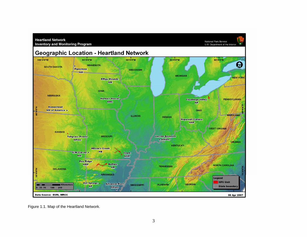
Figure 1.1. Map of the Heartland Network .................................................................................. 3 Figure 2.1. Mean annual precipitation, 1961–1990, for the HTLN ........................................... 12 Figure 2.2. Mean annual snowfall, 1961–1990, for the HTLN .................................................. 13 Figure 2.3. Mean monthly precipitation at selected locations in the HTLN .............................. 14 Figure 2.4. Mean annual temperature, 1961–1990, for the HTLN ............................................ 15 Figure 2.5. Mean January minimum temperature, 1961–1990, for the HTLN .......................... 16 Figure 2.6. Mean July maximum temperature, 1961–1990, for the HTLN ............................... 17 Figure 2.7. Precipitation time series, 1895-2005, for selected regions

in the HTLN ............................................................................................................. 18 Figure 2.8. Temperature time series, 1895-2005, for selected regions

in the HTLN ............................................................................................................. 19 Figure 4.1. Station locations for the HTLN park units in Iowa .................................................. 31 Figure 4.2. Station locations for the HTLN park units in Kansas, Nebraska,

and Minnesota .......................................................................................................... 35 Figure 4.3. Station locations for the HTLN park units in Arkansas

and Missouri ............................................................................................................. 43 Figure 4.4. Station locations for the HTLN park units in Indiana

and Ohio ................................................................................................................... 51

vi

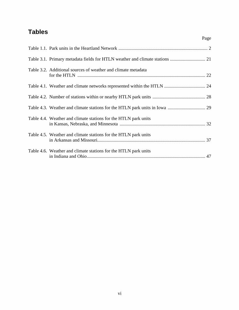
Tables Page

Table 1.1. Park units in the Heartland Network ............................................................................ 2 Table 3.1. Primary metadata fields for HTLN weather and climate stations .............................. 21 Table 3.2. Additional sources of weather and climate metadata

for the HTLN ............................................................................................................. 22 Table 4.1. Weather and climate networks represented within the HTLN ................................... 24 Table 4.2. Number of stations within or nearby HTLN park units ............................................. 28 Table 4.3. Weather and climate stations for the HTLN park units in Iowa ................................ 29 Table 4.4. Weather and climate stations for the HTLN park units

in Kansas, Nebraska, and Minnesota ......................................................................... 32 Table 4.5. Weather and climate stations for the HTLN park units

in Arkansas and Missouri............................................................................................ 37 Table 4.6. Weather and climate stations for the HTLN park units

in Indiana and Ohio..................................................................................................... 47

vii

Appendixes Page

Appendix A. Glossary ............................................................................................................... 60 Appendix B. Climate-monitoring principles ............................................................................. 62 Appendix C. Factors in operating a climate network ................................................................ 65 Appendix D. General design considerations for weather/climate-monitoring programs .......... 68 Appendix E. Master metadata field list ..................................................................................... 88 Appendix F. Electronic supplements ........................................................................................ 90 Appendix G. Descriptions of weather/climate-monitoring networks ........................................ 91

viii

Acronyms AASC American Association of State Climatologists ACIS Applied Climate Information System ARPO Arkansas Post National Monument ASOS Automated Surface Observing System AWDN Automated Weather Data Network AWOS Automated Weather Observing System BLM Bureau of Land Management BUFF Buffalo National River CASTNet Clean Air Status and Trends Network COOP Cooperative Observer Program CRN Climate Reference Network CUVA Cuyahoga Valley National Park CWOP Citizen Weather Observer Program DFIR Double-Fence Intercomparison Reference DRI Desert Research Institute DST daylight savings time EFMO Effigy Mounds National Monument ENSO El Niño Southern Oscillation EPA Environmental Protection Agency FAA Federal Aviation Administration FIPS Federal Information Processing Standards GMT Greenwich Mean Time GOES Geostationary Operational Environmental Satellite GPMP NPS Gaseous Pollutant Monitoring Program GPS Global Positioning System GPS-MET NOAA ground-based GPS meteorology network GWCA George Washington Carver National Monument HEHO Herbert Hoover National Historic Site HOCU Hopewell Culture National Historical Park HOME Homestead National Monument of America HOSP Hot Springs National Park HPRCC High Plains Regional Climate Center HTLN Heartland Inventory and Monitoring Network I&M NPS Inventory and Monitoring Program LEO Low Earth Orbit LIBO Lincoln Boyhood National Monument LST local standard time MDN Mercury Deposition Network NADP National Atmospheric Deposition Program NASA National Aeronautics and Space Administration NCDC National Climatic Data Center NetCDF Network Common Data Form NOAA National Oceanic and Atmospheric Administration NPS National Park Service

ix

NRCS Natural Resources Conservation Service NWS National Weather Service OZAR Ozark National Scenic Riverways PERI Pea Ridge National Military Park PIPE Pipestone National Monument PRISM Parameter Regression on Independent Slopes Model RAWS Remote Automated Weather Station network RCC regional climate center SAO Surface Airways Observation network SCAN Soil Climate Analysis Network SOD Summary Of the Day Surfrad Surface Radiation Budget network SNOTEL Snowfall Telemetry network TAPR Tallgrass Prairie National Preserve UPR Union Pacific Railroad network USDA U.S. Department of Agriculture USGS U.S. Geological Survey UTC Coordinated Universal Time WBAN Weather Bureau Army Navy WICR Wilson’s Creek National Battlefield WIDOT Wisconsin Department of Transportation network WMO World Meteorological Organization WRCC Western Regional Climate Center WX4U Weather For You network

x

Executive Summary Climate is a dominant factor driving the physical and ecologic processes affecting the Heartland Inventory and Monitoring Network (HTLN). The HTLN encompasses a wide range of climates but generally displays a mid-continental climate with temperatures that can vary widely between summer highs and winter lows. Winters in the HTLN are typically dry and cold, while summers are typically warm and humid, especially to the south. The western portions of the HTLN are characterized by highly variable and stormy weather patterns and support the tall-grass prairies of the eastern Great Plains. During the late summer and autumn months, remnants of tropical systems can move north out of the Gulf of Mexico and bring heavy rainfall to southern and eastern portions of the HTLN. Due to the significant variability exhibited by HTLN climate, the region is prone both to severe droughts (e.g., summer of 1988) and catastrophic flooding events (e.g., summer of 1993). There are concerns about how the frequency of drought and flood cycles in the HTLN will change in response to future climate changes and the impacts these changes will have on HTLN ecosystems. The relationship between climate and land-use patterns in the HTLN is also important. Human influences in the HTLN, including highly-fragmented land-use patterns, introduce local microclimate and regional climate changes that in turn lead to local- and regional-scale changes in HTLN ecosystems. The HTLN network has stressed the importance of site-specific weather and climate monitoring. Climate is one of the 12 basic inventories to be completed for all National Park Service (NPS) Inventory and Monitoring Program (I&M) networks. This project was initiated to inventory past and present climate monitoring efforts in the HTLN. In this report, we provide the following information:

• Overview of broad-scale climatic factors and zones important to HTLN park units. • Inventory of weather and climate station locations in and near HTLN park units relevant to

the NPS I&M Program. • Results of an inventory of metadata on each weather station, including affiliations for

weather-monitoring networks, types of measurements recorded at these stations, and information about the actual measurements (length of record, etc.).

• Initial evaluation of the adequacy of coverage for existing weather stations and recommendations for improvements in monitoring weather and climate.

Precipitation in the HTLN region increases from northwest to southeast, dictated by proximity to moist flows from the Gulf of Mexico. Mean annual precipitation ranges from just over 600 mm at Pipestone National Monument (PIPE) to almost 1500 mm at Hot Springs National Park (HOSP). Mean annual snowfall can approach 100 cm at some northern HTLN park units like PIPE and Cuyahoga Valley National Park (CUVA). The seasonal cycle of precipitation in HTLN park units varies greatly around the network. For example, the Great Plains see a marked precipitation maximum during the summer months, while to the south, in Arkansas, precipitation peaks occur both in late spring and in late autumn/early winter. Mean annual temperatures across the HTLN increase from north to south, ranging from just below 7°C at PIPE to over 15°C at Arkansas Post National Monument (ARPO). Mean winter minimum temperatures approach -20°C in some northern park units (e.g., PIPE), while mean summer maximum temperatures can exceed 32°C in Arkansas park units.

xi

Through a search of national databases and inquiries to NPS staff, we have identified 23 weather and climate stations within HTLN park units. Ozark National Scenic Riverways (OZAR) has the most stations within park boundaries (7). Most of the weather and climate stations we identified had metadata and data records that are sufficiently complete and satisfactory in quality. The HTLN network is committed to improving the weather- and climate-monitoring activities within their park units. In fact, the HTLN network has already identified weather and climate stations in and near each of the HTLN park units for which data are being ingested. The monitoring of climate variations at longer time scales and their impacts on HTLN plant and animal communities is assisted by the availability of reliable long-term climate records in or near most HTLN park units, including the climate data currently being ingested by HTLN. However, climate variations at shorter time scales, including extreme events with high spatial variability (e.g., thunderstorm precipitation), are not sampled well by the existing coverage of weather and climate stations. Few near-real-time weather and climate stations were identified within the park units themselves. This is particularly critical for Buffalo National River (BUFF) and OZAR. The only near-real-time stations we identified in BUFF are located in the eastern part of the park unit. There are no near-real-time weather stations in OZAR currently. Both BUFF and OZAR protect riverways that provide opportunities for setting up local climate transect measurements. Such transects would help to document spatial variations of extreme weather events and the associated disturbances that impact these relatively-pristine riverways. At BUFF, for instance, a Remote Automated Weather Station (RAWS) installation in the western portion of the park unit would complement the existing RAWS sites in eastern BUFF. As an additional strategy for documenting the spatial characteristics of extreme weather and climate events in the HTLN, The NPS could encourage greater coverage of near-real-time weather stations outside of HTLN park units. Station networks such as the Automated Weather Data Network (AWDN), RAWS, and the Soil Climate Analysis Network (SCAN) each have a presence in the HTLN region and NPS could work with agencies such as the High Plains Regional Climate Center (HPRCC) for AWDN and the Natural Resources Conservation Service (NRCS) for the SCAN network to encourage new weather station installations in or near HTLN park units.

xii

Acknowledgements This work was supported and completed under Task Agreement H8R07010001, with the Great Basin Cooperative Ecosystem Studies Unit. We would like to acknowledge very helpful assistance from various National Park Service personnel associated with the Heartland Inventory and Monitoring Network. Particular thanks are extended to Mike DeBacker and David Peitz. We also thank John Gross, Margaret Beer, Grant Kelly, Greg McCurdy, and Heather Angeloff for all their help. Seth Gutman with the National Oceanic and Atmospheric Administration Earth Systems Research Laboratory provided valuable input on the GPS-MET station network. Portions of the work were supported by the NOAA Western Regional Climate Center.

1

1.0. Introduction Weather and climate are key drivers in ecosystem structure and function. Global- and regional-scale climate variations will have a tremendous impact on natural systems (Chapin et al. 1996; Schlesinger 1997; Jacobson et al. 2000; Bonan 2002). Long-term patterns in temperature and precipitation provide first-order constraints on potential ecosystem structure and function. Secondary constraints are realized from the intensity and duration of individual weather events and, additionally, from seasonality and inter-annual climate variability. These constraints influence the fundamental properties of ecologic systems, such as soil–water relationships, plant–soil processes, and nutrient cycling, as well as disturbance rates and intensity. These properties, in turn, influence the life-history strategies supported by a climatic regime (Neilson 1987; Rodriguez-Iturbe 2000; DeBacker et al. 2005). Given the importance of climate, it is one of 12 basic inventories to be completed by the National Park Service (NPS) Inventory and Monitoring Program (I&M) network (I&M 2006). As primary environmental drivers for the other vital signs, weather and climate patterns present various practical and management consequences and implications for the NPS (Oakley et al. 2003). Most park units observe weather and climate elements as part of their overall mission. The lands under NPS stewardship provide many excellent locations for monitoring climatic conditions. It is essential that park units within the Heartland Inventory and Monitoring Network (HTLN) have an effective climate-monitoring system in place to track climate changes and to aid in management decisions relating to these changes. The purpose of this report is to determine the current status of weather and climate monitoring within the HTLN (Table 1.1; Figure 1.1). In this report, we provide the following informational elements:

• Overview of broad-scale climatic factors and zones important to HTLN park units. • Inventory of locations for all weather stations in and near HTLN park units that are relevant

to the NPS I&M networks. • Results of metadata inventory for each station, including weather-monitoring network

affiliations, types of recorded measurements, and information about actual measurements (length of record, etc.).

• Initial evaluation of the adequacy of coverage for existing weather stations and recommendations for improvements in monitoring weather and climate.

The primary objective of climate- and weather-monitoring activities in HTLN is to understand how climate variation across the midwestern U.S. affects HTLN parks. In particular, HTLN climate-monitoring efforts intend to determine how climatic factors affecting plant and animal populations, communities, and aquatic systems vary seasonally and annually (DeBacker et al. 2005). 1.1. Network Terminology Before proceeding, it is important to stress that this report discusses the idea of “networks” in two different ways. Modifiers are used to distinguish between NPS I&M networks and weather/climate station networks. See Appendix A for a full definition of these terms.

2

1.1.1. Weather and climate Station Networks Most weather and climate measurements are made not from isolated stations but from stations that are part of a network operated in support of a particular mission. The limiting case is a network of one station, where measurements are made by an interested observer or group. Larger networks usually have additional inventory data and station-tracking procedures. Some national weather and climate networks are associated with the National Oceanic and Atmospheric Administration (NOAA), including the National Weather Service (NWS) Cooperative Observer Program (COOP). Other national networks include the interagency Remote Automated Weather Station network (RAWS) and the U.S. Department of Agriculture/Natural Resources Conservation Service (USDA/NRCS) Soil Climate Analysis Network (SCAN). Usually a single agency, but sometimes a consortium of interested parties, will jointly support a particular weather/climate network. Table 1.1. Park units in the Heartland Network.

Acronym Name ARPO Arkansas Post National Monument BUFF Buffalo National River CUVA Cuyahoga Valley National Park EFMO Effigy Mounds National Monument GWCA George Washington Carver National Monument HEHO Herbert Hoover National Historic Site HOCU Hopewell Culture National Historical Park HOME Homestead National Monument of America HOSP Hot Springs National Park LIBO Lincoln Boyhood National Monument OZAR Ozark National Scenic Riverways PERI Pea Ridge National Military Park PIPE Pipestone National Monument TAPR Tallgrass Prairie National Preserve WICR Wilson’s Creek National Battlefield

1.1.2. NPS I&M Networks Within the NPS, the system for monitoring various attributes in the participating park units (about 270–280 in total) is divided into 32 NPS I&M networks. These networks are collections of park units grouped together around a common theme, typically geographical. 1.2. Weather versus Climate Definitions It is also important to distinguish whether the primary use of a given station is for weather purposes or for climate purposes. Weather station networks are intended for near-real-time

3

Figure 1.1. Map of the Heartland Network.

4

usage, where the precise circumstances of a set of measurements are typically less important. In these cases, changes in exposure or other attributes over time are not as critical. Climate networks, however, are intended for long-term tracking of atmospheric conditions. Siting and exposure are critical factors for climate networks, and it is vitally important that the observational circumstances remain essentially unchanged over the duration of the station record. Some climate networks can be considered hybrids of weather and climate networks. These hybrid climate networks can supply information on a short-term “weather” time scale and a longer-term “climate” time scale. In this report, “weather” generally refers to current (or near-real-time) atmospheric conditions, while “climate” is defined as the complete ensemble of statistical descriptors for temporal and spatial properties of atmospheric behavior (see Appendix A). Climate and weather phenomena shade gradually into each other and are ultimately inseparable. 1.3. Purpose of Measurements Climate inventory and monitoring climate activities should be based on a set of guiding fundamental principles. Any evaluation of weather and climate monitoring programs begins with asking the following question:

• What is the purpose of weather and climate measurements? Evaluation of past, present, or planned weather and climate monitoring activities must be based on the answer to this question. Weather and climate data and information constitute a prominent and widely requested component of the NPS I&M networks (I&M 2006). Within the context of the NPS, the following services constitute the main purposes for recording weather and climate observations:

• Provide measurements for real-time operational needs and early warnings of potential hazards (landslides, mudflows, washouts, fallen trees, plowing activities, fire conditions, aircraft and watercraft conditions, road conditions, rescue conditions, fog, restoration and remediation activities, etc.).

• Provide visitor education and aid interpretation of expected and actual conditions for visitors while they are in the park and for deciding if and when to visit the park.

• Establish engineering and design criteria for structures, roads, culverts, etc., for human comfort, safety, and economic needs.

• Consistently monitor climate over the long-term to detect changes in environmental drivers affecting ecosystems, including both gradual and sudden events.

• Provide retrospective data to understand a posteriori changes in flora and fauna. • Document for posterity the physical conditions in and near the park units, including mean,

extreme, and variable measurements (in time and space) for all applications. The last three items in the preceding list are pertinent primarily to the NPS I&M networks; however, all items are important to NPS operations and management. Most of the needs in this list overlap heavily. It is often impractical to operate separate climate measuring systems that

5

also cannot be used to meet ordinary weather needs, where there is greater emphasis on timeliness and reliability. 1.4. Design of Climate-Monitoring Programs Determining the purposes for collecting measurements in a given weather/climate monitoring program will guide the process of identifying weather and climate stations suitable for the monitoring program. The context for making these decisions is provided in Chapter 2 where background on the HTLN climate is presented. However, this process is only one step in evaluating and designing a climate-monitoring program. The following steps must also be included:

• Define park and network-specific monitoring needs and objectives. • Identify locations and data repositories of existing and historic stations. • Acquire existing data when necessary or practical. • Evaluate the quality of existing data. • Evaluate the adequacy of coverage of existing stations. • Develop a protocol for monitoring the weather and climate, including the following:

o Standardized summaries and reports of weather and climate data. o Data management (quality assurance and quality control, archiving, data access, etc.).

• Develop and implement a plan for installing or modifying stations, as necessary. Throughout the design process, there are various factors that require consideration in evaluating weather and climate measurements. Many of these factors have been summarized by Dr. Tom Karl, director of the NOAA National Climatic Data Center (NCDC), and widely distributed as the “Ten Principles for Climate Monitoring” (Karl et al. 1996; NRC 2001). These principles are presented in Appendix B, and the guidelines are embodied in many of the comments made throughout this report. The most critical factors are presented here. In addition, an overview of requirements necessary to operate a climate network is provided in Appendix C, with further discussion in Appendix D. 1.4.1. Need for Consistency A principal goal in climate monitoring is to detect and characterize slow and sudden changes in climate through time. This is of less concern for day-to-day weather changes, but it is of paramount importance for climate variability and change. There are many ways whereby changes in techniques for making measurements, changes in instruments or their exposures, or seemingly innocuous changes in site characteristics can lead to apparent changes in climate. Safeguards must be in place to avoid these false sources of temporal “climate” variability if we are to draw correct inferences about climate behavior over time from archived measurements. For climate monitoring, consistency through time is vital, counting at least as important as absolute accuracy. Sensors record only what is occurring at the sensor—this is all they can detect. It is the responsibility of station or station network managers to ensure that observations are representative of the spatial and temporal climate scales that we wish to record. 1.4.2. Metadata

6

Changes in instruments, site characteristics, and observing methodologies can lead to apparent changes in climate through time. It is therefore vital to document all factors that can bear on the interpretation of climate measurements and to update the information repeatedly through time. This information (“metadata,” data about data) has its own history and set of quality-control issues that parallel those of the actual data. There is no single standard for the content of climate metadata, but a simple rule suffices:

• Observers should record all information that could be needed in the future to interpret observations correctly without benefit of the observers’ personal recollections.

Such documentation includes notes, drawings, site forms, and photos, which can be of inestimable value if taken in the correct manner. That stated, it is not always clear to the metadata provider what is important for posterity and what will be important in the future. It is almost impossible to “over document” a station. Station documentation is greatly underappreciated and is seldom thorough enough (especially for climate purposes). Insufficient attention to this issue often lowers the present and especially future value of otherwise useful data. The convention followed throughout climatology is to refer to metadata as information about the measurement process, station circumstances, and data. The term “data” is reserved solely for the actual weather and climate records obtained from sensors. 1.4.3. Maintenance Inattention to maintenance is the greatest source of failure in weather and climate stations and networks. Problems begin to occur soon after sites are deployed. A regular visit schedule must be implemented, where sites, settings (e.g., vegetation), sensors, communications, and data flow are checked routinely (once or twice a year at a minimum) and updated as necessary. Parts must be changed out for periodic recalibration or replacement. With adequate maintenance, the entire instrument suite should be replaced or completely refurbished about once every five to seven years. Simple preventive maintenance is effective but requires much planning and skilled technical staff. Changes in technology and products require retraining and continual re-education. Travel, logistics, scheduling, and seasonal access restrictions consume major amounts of time and budget but are absolutely necessary. Without such attention, data gradually become less credible and then often are misused or not used at all. 1.4.4. Automated versus Manual Stations Historic stations often have depended on manual observations and many continue to operate in this mode. Manual observations frequently produce excellent data sets. Sensors and data are simple and intuitive, well tested, and relatively cheap. Manual stations have much to offer in certain circumstances and can be a source of both primary and backup data. However, methodical consistency for manual measurements is a constant challenge, especially with a mobile work force. Operating manual stations takes time and needs to be done on a regular schedule, though sometimes the routine is welcome.

7

Nearly all newer stations are automated. Automated stations provide better time resolution, increased (though imperfect) reliability, greater capacity for data storage, and improved accessibility to large amounts of data. The purchase cost for automated stations is higher than for manual stations. A common expectation and serious misconception is that an automated station can be deployed and left to operate on its own. In reality, automation does not eliminate the need for people but rather changes the type of person that is needed. Skilled technical personnel are needed and must be readily available, especially if live communications exist and data gaps are not wanted. Site visits are needed at least annually and spare parts must be maintained. Typical annual costs for sensors and maintenance are $1500–2500 per station per year. 1.4.5. Communications With manual stations, the observer is responsible for recording and transmitting station data. Data from automated stations, however, can be transmitted quickly for access by research and operations personnel, which is a highly preferable situation. A comparison of communication systems for automated and manual stations shows that automated stations generally require additional equipment, more power, higher transmission costs, attention to sources of disruption or garbling, and backup procedures (e.g., manual downloads from data loggers). Automated stations are capable of functioning normally without communication and retaining many months of data. At such sites, however, alerts about station problems are not possible, large gaps can accrue when accessible stations quit, and the constituencies needed to support such stations are smaller and less vocal. Two-way communications permit full recovery from disruptions, ability to reprogram data loggers remotely, and better opportunities for diagnostics and troubleshooting. In virtually all cases, two-way communications are much preferred to all other communication methods. However, two-way communications require considerations of cost, signal access, transmission rates, interference, and methods for keeping sensor and communication power loops separate. Two-way communications are frequently impossible (no service) or impractical, expensive, or power consumptive. Two-way methods (cellular, land line, radio, Internet) require smaller up-front costs as compared to other methods of communication and have variable recurrent costs, starting at zero. Satellite links work everywhere (except when blocked by trees or cliffs) and are quite reliable but are one-way and relatively slow, allow no re-transmissions, and require high up-front costs ($3000–4000) but no recurrent costs. Communications technology is changing constantly and requires vigilant attention by maintenance personnel. 1.4.6. Quality Assurance and Quality Control Quality control and quality assurance are issues at every step through the entire sequence of sensing, communication, storage, retrieval, and display of environmental data. Quality assurance is an umbrella concept that covers all data collection and processing (start-to-finish) and ensures that credible information is available to the end user. Quality control has a more limited scope and is defined by the International Standards Organization as “the operational techniques and activities that are used to satisfy quality requirements.” The central problem can be better appreciated if we approach quality control in the following way.

• Quality control is the evaluation, assessment, and rehabilitation of imperfect data by utilizing other imperfect data.

8

The quality of the data only decreases with time once the observation is made. The best and most effective quality control, therefore, consists in making high-quality measurements from the start and then successfully transmitting the measurements to an ingest process and storage site. Once the data are received from a monitoring station, a series of checks with increasing complexity can be applied, ranging from single-element checks (self-consistency) to multiple-element checks (inter-sensor consistency) to multiple-station/single-element checks (inter-station consistency). Suitable ancillary data (battery voltages, data ranges for all measurements, etc.) can prove extremely useful in diagnosing problems. There is rarely a single technique in quality control procedures that will work satisfactorily for all situations. Quality-control procedures must be tailored to individual station circumstances, data access and storage methods, and climate regimes. The fundamental issue in quality control centers on the tradeoff between falsely rejecting good data (Type I error) and falsely accepting bad data (Type II error). We cannot reduce the incidence of one type of error without increasing the incidence of the other type. In weather and climate data assessments, since good data are absolutely crucial for interpreting climate records properly, Type I errors are deemed far less desirable than Type II errors. Not all observations are equal in importance. Quality-control procedures are likely to have the greatest difficulty evaluating the most extreme observations, where independent information usually must be sought and incorporated. Quality-control procedures involving more than one station usually involve a great deal of infrastructure with its own (imperfect) error-detection methods, which must be in place before a single value can be evaluated. 1.4.7. Standards Although there is near-universal recognition of the value in systematic weather and climate measurements, these measurements will have little value unless they conform to accepted standards. There is not a single source for standards for collecting weather and climate data nor a single standard that meets all needs. Measurement standards have been developed by the World Meteorological Organization (WMO 1983; 2005), the American Association of State Climatologists (AASC 1985), the U.S. Environmental Protection Agency (EPA 1987), Finklin and Fischer (1990), the RAWS program (Bureau of Land Management [BLM] 1997), and the National Wildfire Coordinating Group (2004). Variations to these measurement standards also have been offered by instrument makers (e.g., Tanner 1990). 1.4.8. Who Makes the Measurements? The lands under NPS stewardship provide many excellent locations to host the monitoring of climate by the NPS or other collaborators. These lands are largely protected from human development and other land changes that can impact observed climate records. Most park units historically have observed weather and climate elements as part of their overall mission. Many of these measurements come from station networks managed by other agencies, with observations taken or overseen by NPS personnel, in some cases, or by collaborators from the other agencies. Any NPS park units that are small, lack sufficient resources, or lack sites presenting adequate

9

exposure may benefit by utilizing weather and climate measurements collected from nearby stations.

10

2.0. Climate Background Climate is a primary driver of almost all physical and ecological processes in the HTLN (DeBacker et al. 2005). It is essential that the HTLN park units have an effective climate monitoring system to track climate changes and to aid in management decisions relating to these changes. In order to do this, it is essential to understand the climate characteristics of the HTLN, as discussed in this chapter. 2.1. Climate and the HTLN Environment The HTLN, due to its large areal extent, encompasses a wide range of climates (DeBacker et al. 2005). In general, however, the HTLN region has a mid-continental climate with temperatures that can vary widely between summer highs and winter lows. Winters in the HTLN are typically dry and cold. During the summer, warm and humid conditions dominate, especially in the southern portions of the network. The western portions of the network lie in the eastern Great Plains, a region that is typified by highly variable and stormy weather patterns. Air masses in this portion of the HTLN are generally drier and become more moisture-laden as they move east and experience increasing interaction with more humid air masses from the Gulf of Mexico. These climate characteristics support the tall-grass prairies of the eastern plains (DeBacker et al. 2005; Perkins et al. 2005). During the late summer and autumn months, remnants of tropical systems can move north out of the Gulf of Mexico and bring heavy rainfall to southern and eastern portions of the HTLN. Due to the significant variability exhibited by HTLN climate, the region is prone both to severe droughts and catastrophic flooding events (Namias 1982; Trenberth et al. 1988; Giorgi et al. 1996; Trenberth and Guillemot 1996). Examples of droughts that have had large consequences for the HTLN region include the Dust Bowl of the 1930s and the devastating drought of the summer of 1988 (Trenberth et al. 1988). Well-known flooding events in the HTLN include the summer of 1993 (Kunkel et al. 1994). There are concerns about how the frequency of drought and flood cycles in the HTLN will change in response to future climate changes (DeBacker et al. 2005). Any such changes will have significant impacts on HTLN ecosystems and will therefore have park management consequences for HTLN park units. The relationship between climate and land-use patterns in the HTLN is also important. In addition to introducing habitat fragmentation and decreasing biodiversity in the HTLN (DeBacker et al. 2005), land use changes in the HTLN region also introduce local microclimate and regional climate changes that in turn lead to local- and regional-scale changes in HTLN ecosystems. Human impacts are also threatening native plants communities in the HTLN with the introduction of invasive plant species (DeBacker et al. 2005). Climate variations will have a direct influence on the rates of spread of these invasive species, and the abilities of native plant communities to respond to the introduction of non-native species. 2.2. Parameter Regression on Independent Slopes Model The climate maps presented in this report were generated using the Parameter Regression on Independent Slopes Model (PRISM). This model was developed to address the extreme spatial and elevation gradients exhibited by the climate of the U.S. (Daly et al. 1994; 2002; Gibson et al. 2002; Doggett et al. 2004). The maps produced through PRISM have undergone rigorous

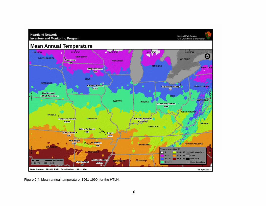
11

evaluation in the U.S. This model was originally developed to provide climate information at scales matching available land-cover maps to assist in ecologic modeling. The PRISM technique accounts for the scale-dependent effects of topography on mean values of climate elements. Elevation provides the first-order constraint for the mapped climate fields, with slope and orientation (aspect) providing second-order constraints. The model has been enhanced gradually to address inversions, coast/land gradients, and climate patterns in small-scale trapping basins. Monthly climate fields are generated by PRISM to account for seasonal variations in elevation gradients in climate elements. These monthly climate fields then can be combined into seasonal and annual climate fields. Since PRISM maps are grid maps, they do not replicate point values but rather, for a given grid cell, represent the grid-cell average of the climate variable in question at the average elevation for that cell. The model relies on observed surface and upper-air measurements to estimate spatial climate fields. 2.3. Spatial Variability Precipitation in the HTLN region generally increases from northwest to southeast across the network, dictated by proximity to moist flows from the Gulf of Mexico (DeBacker et al. 2005). Mean annual precipitation, as estimated from PRISM, ranges from just over 600 mm in PIPE to almost 1500 mm in HOSP (Figure 2.1). Snowfall, on the other hand, increases from south to north, with estimated mean annual snowfalls approaching 100 cm at both PIPE and CUVA (Figure 2.2). The snowiest locations are closest to the Great Lakes. The seasonal cycle of precipitation in HTLN park units varies greatly around the network (Figure 2.3). To the west, in the Great Plains, precipitation displays a sharper maximum during the summer months (e.g., Figure 2.3a) as compared to locations further east, such as Ohio (e.g., Figure 2.3c), where a summer precipitation maximum still occurs but it is less distinct. To the south, in Arkansas, precipitation shows two maxima, one in late spring and the other in late autumn/early winter (Figure 2.3b). Mean annual temperatures across the HTLN increase from north to south (Figure 2.4). The coldest conditions are found at PIPE, where mean annual temperatures as estimated from PRISM are just below 7°C. In contrast, the warmest conditions are found at ARPO, where estimated mean annual temperatures exceed 15°C. The north-south temperature gradient is also apparent when looking at mean January minimum temperatures (Figure 2.5), which are coolest for PIPE (-19°C) and warmest for ARPO (above -4°C). Summer maximum temperatures are warmest in the Great Plains and Lower Mississippi River Valley but are coolest in areas closest to the Great Lakes. The coolest park unit, CUVA, sees July maximum temperatures that are estimated to be below 28°C. On the other hand, park units such as HOSP and ARPO see July maximum temperatures that are well above 32°C (Figure 2.6). 2.3. Temporal Variability The HTLN climate displays significant temporal variability at scales ranging from days to years. A significant driver of the interannual climate variations in the HTLN is the El Niño Southern Oscillation, or ENSO (Bunkers et al. 1996; NAST 2001), which influences HTLN weather particularly during the winter months. In northern HTLN, El Niño conditions (warm ENSO phases) are associated with drier weather and temperatures that are warmer than average during the winter months, while La Niña conditions (cool ENSO phases) are associated with colder temperatures and more precipitation (mostly snowfall). To the south, the situation begins to

12

reverse, with El Niño conditions bringing cooler and wetter weather compared to normal and La Niña conditions bringing drier, warmer weather compared to normal. An investigation of precipitation time series around the HTLN region over the last century (Figure 2.7) reveals little in the way of an overall trend. Precipitation over the Great Plains and in portions of Ohio appears to have increased slightly, while precipitation in Arkansas shows no trend. The wet summer of 1993 is evident in the precipitation time series for east-central Iowa (Figure 2.7a). Long-term temperature trends are quite variable around the HTLN (Figure 2.8). Some locations, such as east-central Iowa and northeast Ohio, indicate a slight warming trend over the past century. However, temperature time series for Arkansas show no overall trend during the past 100 years but rather show distinct warm cycles, such as those in the 1920s and 1930s, and distinct cool cycles, such as those in the 1960s and 1970s.

13

Figure 2.1. Mean annual precipitation, 1961-1990, for the HTLN.

14

Figure 2.2. Mean annual snowfall, 1961-1990, for the HTLN.

15

a)

b)

c)

Figure 2.3. Mean monthly precipitation at selected locations in the HTLN. Locations include Iowa City 1 S, near HEHO (a); Hot Springs 1 NNE, near HOSP (b), and Akron-Canton Airport, near CUVA (c).

16

Figure 2.4. Mean annual temperature, 1961-1990, for the HTLN.

17

Figure 2.5. Mean January minimum temperature, 1961-1990, for the HTLN.

18

Figure 2.6. Mean July maximum temperature, 1961-1990, for the HTLN.

19

a)

b)

c)

Figure 2.7. Precipitation time series, 1895-2005, for selected regions in the HTLN. These include twelve-month precipitation (ending in December) (red), 10-year running mean (blue), mean (green), and plus/minus one standard deviation (green dotted). Locations include east-central Iowa (a), central Arkansas (b), and northeastern Ohio (c).

20

a)

b)

c)

Figure 2.8. Temperature time series, 1895-2005, for selected regions in the HTLN. These include twelve-month average temperature (ending in December) (red), 10-year running mean (blue), mean (green), and plus/minus one standard deviation (green dotted). Locations include east-central Iowa (a), central Arkansas (b), and northeastern Ohio (c).

21

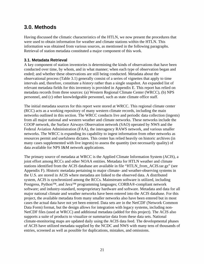
3.0. Methods Having discussed the climatic characteristics of the HTLN, we now present the procedures that were used to obtain information for weather and climate stations within the HTLN. This information was obtained from various sources, as mentioned in the following paragraphs. Retrieval of station metadata constituted a major component of this work. 3.1. Metadata Retrieval A key component of station inventories is determining the kinds of observations that have been conducted over time, by whom, and in what manner; when each type of observation began and ended; and whether these observations are still being conducted. Metadata about the observational process (Table 3.1) generally consist of a series of vignettes that apply to time intervals and, therefore, constitute a history rather than a single snapshot. An expanded list of relevant metadata fields for this inventory is provided in Appendix E. This report has relied on metadata records from three sources: (a) Western Regional Climate Center (WRCC), (b) NPS personnel, and (c) other knowledgeable personnel, such as state climate office staff. The initial metadata sources for this report were stored at WRCC. This regional climate center (RCC) acts as a working repository of many western climate records, including the main networks outlined in this section. The WRCC conducts live and periodic data collection (ingests) from all major national and western weather and climate networks. These networks include the COOP network, the Surface Airways Observation network (SAO) operated by NWS and the Federal Aviation Administration (FAA), the interagency RAWS network, and various smaller networks. The WRCC is expanding its capability to ingest information from other networks as resources permit and usefulness dictates. This center has relied heavily on historic archives (in many cases supplemented with live ingests) to assess the quantity (not necessarily quality) of data available for NPS I&M network applications. The primary source of metadata at WRCC is the Applied Climate Information System (ACIS), a joint effort among RCCs and other NOAA entities. Metadata for HTLN weather and climate stations identified from the ACIS database are available in file “HTLN_from_ACIS.tar.gz” (see Appendix F). Historic metadata pertaining to major climate- and weather-observing systems in the U.S. are stored in ACIS where metadata are linked to the observed data. A distributed system, ACIS is synchronized among the RCCs. Mainstream software is utilized, including Postgress, Python™, and Java™ programming languages; CORBA®-compliant network software; and industry-standard, nonproprietary hardware and software. Metadata and data for all major national climate and weather networks have been entered into the ACIS database. For this project, the available metadata from many smaller networks also have been entered but in most cases the actual data have not yet been entered. Data sets are in the NetCDF (Network Common Data Form) format, but the design allows for integration with legacy systems, including non-NetCDF files (used at WRCC) and additional metadata (added for this project). The ACIS also supports a suite of products to visualize or summarize data from these data sets. National climate-monitoring maps are updated daily using the ACIS data feed. The developmental phases of ACIS have utilized metadata supplied by the NCDC and NWS with many tens of thousands of entries, screened as well as possible for duplications, mistakes, and omissions.

22

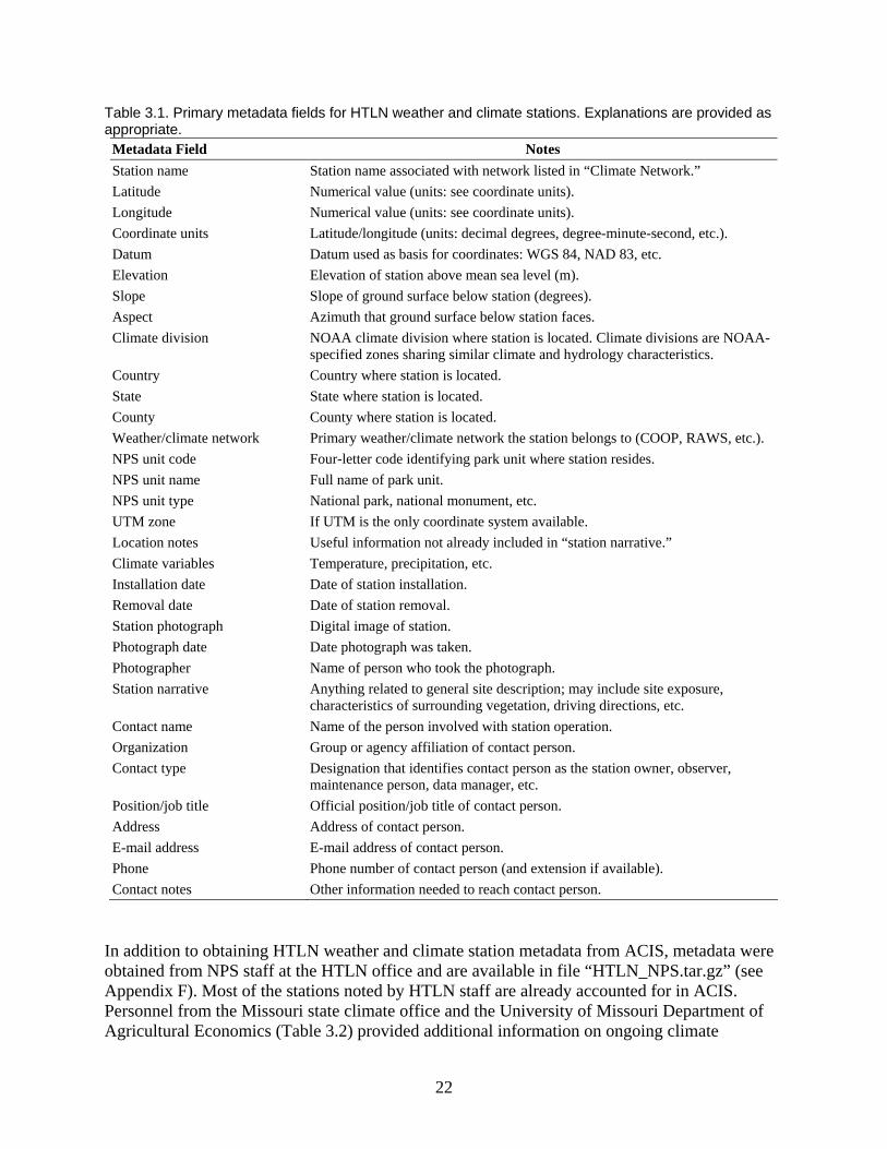
Table 3.1. Primary metadata fields for HTLN weather and climate stations. Explanations are provided as appropriate.

Metadata Field Notes Station name Station name associated with network listed in “Climate Network.” Latitude Numerical value (units: see coordinate units). Longitude Numerical value (units: see coordinate units). Coordinate units Latitude/longitude (units: decimal degrees, degree-minute-second, etc.). Datum Datum used as basis for coordinates: WGS 84, NAD 83, etc. Elevation Elevation of station above mean sea level (m). Slope Slope of ground surface below station (degrees). Aspect Azimuth that ground surface below station faces. Climate division NOAA climate division where station is located. Climate divisions are NOAA-

specified zones sharing similar climate and hydrology characteristics. Country Country where station is located. State State where station is located. County County where station is located. Weather/climate network Primary weather/climate network the station belongs to (COOP, RAWS, etc.). NPS unit code Four-letter code identifying park unit where station resides. NPS unit name Full name of park unit. NPS unit type National park, national monument, etc. UTM zone If UTM is the only coordinate system available. Location notes Useful information not already included in “station narrative.” Climate variables Temperature, precipitation, etc. Installation date Date of station installation. Removal date Date of station removal. Station photograph Digital image of station. Photograph date Date photograph was taken. Photographer Name of person who took the photograph. Station narrative Anything related to general site description; may include site exposure,

characteristics of surrounding vegetation, driving directions, etc. Contact name Name of the person involved with station operation. Organization Group or agency affiliation of contact person. Contact type Designation that identifies contact person as the station owner, observer,

maintenance person, data manager, etc. Position/job title Official position/job title of contact person. Address Address of contact person. E-mail address E-mail address of contact person. Phone Phone number of contact person (and extension if available). Contact notes Other information needed to reach contact person.

In addition to obtaining HTLN weather and climate station metadata from ACIS, metadata were obtained from NPS staff at the HTLN office and are available in file “HTLN_NPS.tar.gz” (see Appendix F). Most of the stations noted by HTLN staff are already accounted for in ACIS. Personnel from the Missouri state climate office and the University of Missouri Department of Agricultural Economics (Table 3.2) provided additional information on ongoing climate

23

monitoring efforts in HTLN. We have also relied on information supplied at various times in the past by the BLM, NPS, NCDC, and NWS. Table 3.2. Additional sources of weather and climate metadata for the HTLN.

Name Position Phone Number Email Address Pat Guinan Missouri State Climatologist,

University of Missouri (573)882-8599 guinanp@missouri.edu

John Travlos Research Scientist, Department of Agricultural Economics, University of Missouri

(573)882-7369 travlosj@missouri.edu

Two types of information have been used to complete the HTLN weather and climate station inventory.

• Station inventories: Information about observational procedures, latitude/longitude, elevation, measured elements, measurement frequency, sensor types, exposures, ground cover and vegetation, data-processing details, network, purpose, and managing individual or agency, etc.

• Data inventories: Information about measured data values including completeness,

seasonality, data gaps, representation of missing data, flagging systems, how special circumstances in the data record are denoted, etc.

This is not a straightforward process. Extensive searches are typically required to develop historic station and data inventories. Both types of inventories frequently contain information gaps and often rely on tacit and unrealistic assumptions. Sources of information for these inventories frequently are difficult to recover or are undocumented and unreliable. In many cases, the actual weather and climate data available from different sources are not linked directly to metadata records. To the extent that actual data can be acquired (rather than just metadata), it is possible to cross-check these records and perform additional assessments based on the amount and completeness of the data. Certain types of weather and climate networks that possess any of the following attributes have not been considered for inclusion in the inventory:

• Private networks with proprietary access and/or inability to provide sufficient metadata. • Private weather enthusiasts (often with high-quality data) whose metadata are not available

and whose data are not readily accessible. • Unofficial observers supplying data to the NWS (lack of access to current data and historic

archives; lack of metadata). • Networks having no available historic data. • Networks having poor-quality metadata. • Networks having poor access to metadata. • Real-time networks having poor access to real-time data.

24

Previous inventory efforts at WRCC have shown that for the weather and climate networks identified in the preceding list, in light of the need for quality data to track weather and climate, the resources required and difficulty encountered in obtaining metadata or data are prohibitively large. 3.2. Criteria for Locating Stations To identify weather and climate stations for each park unit in the HTLN we selected only those stations located within 40 km of the HTLN park units. This buffer distance was selected in an attempt to include automated stations from major networks such as RAWS and SAO, but also to keep the size of the stations lists down to a reasonable number. The station locator maps presented in Chapter 4 were designed to show clearly the spatial distributions of all major weather and climate station networks in HTLN. We recognize that other mapping formats may be more suitable for other specific needs.

25

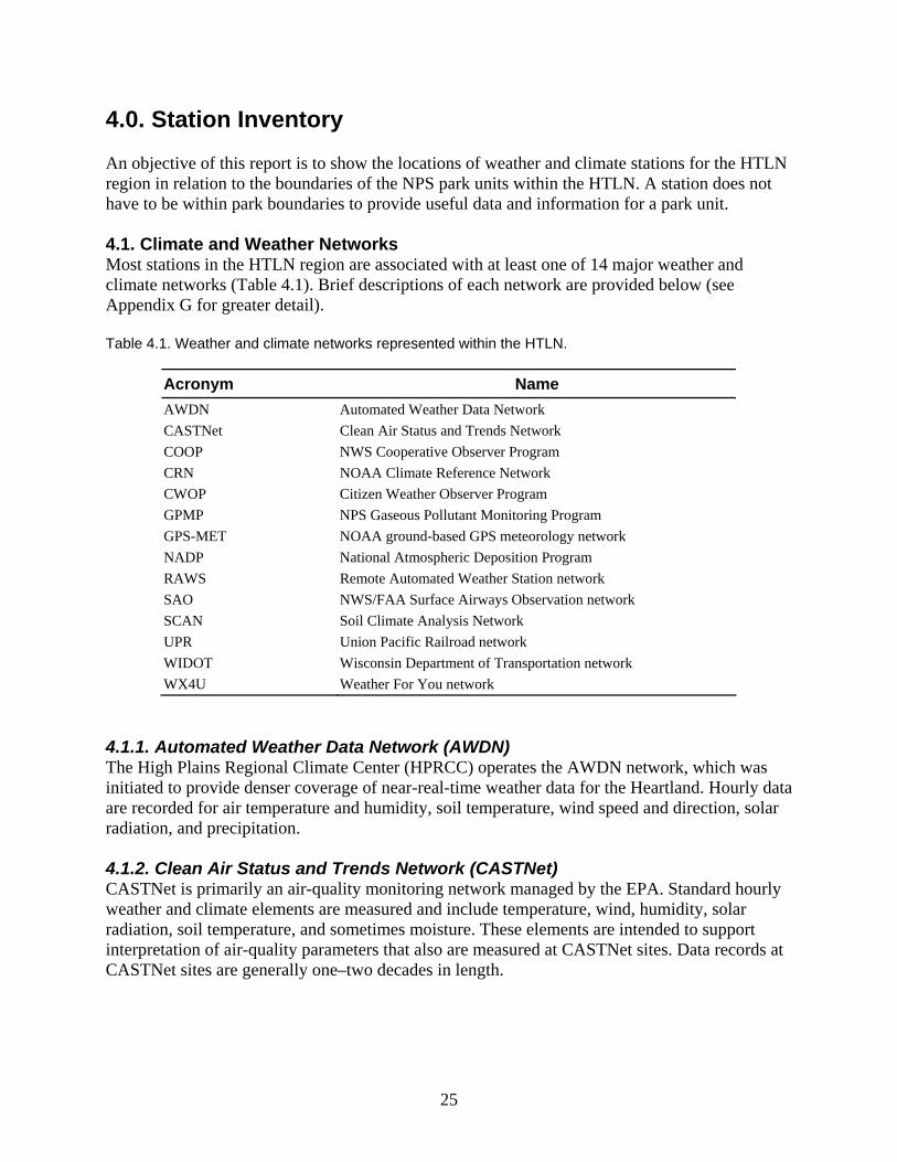
4.0. Station Inventory An objective of this report is to show the locations of weather and climate stations for the HTLN region in relation to the boundaries of the NPS park units within the HTLN. A station does not have to be within park boundaries to provide useful data and information for a park unit. 4.1. Climate and Weather Networks Most stations in the HTLN region are associated with at least one of 14 major weather and climate networks (Table 4.1). Brief descriptions of each network are provided below (see Appendix G for greater detail). Table 4.1. Weather and climate networks represented within the HTLN.

Acronym Name AWDN Automated Weather Data Network CASTNet Clean Air Status and Trends Network COOP NWS Cooperative Observer Program CRN NOAA Climate Reference Network CWOP Citizen Weather Observer Program GPMP NPS Gaseous Pollutant Monitoring Program GPS-MET NOAA ground-based GPS meteorology network NADP National Atmospheric Deposition Program RAWS Remote Automated Weather Station network SAO NWS/FAA Surface Airways Observation network SCAN Soil Climate Analysis Network UPR Union Pacific Railroad network WIDOT Wisconsin Department of Transportation network WX4U Weather For You network

4.1.1. Automated Weather Data Network (AWDN) The High Plains Regional Climate Center (HPRCC) operates the AWDN network, which was initiated to provide denser coverage of near-real-time weather data for the Heartland. Hourly data are recorded for air temperature and humidity, soil temperature, wind speed and direction, solar radiation, and precipitation. 4.1.2. Clean Air Status and Trends Network (CASTNet) CASTNet is primarily an air-quality monitoring network managed by the EPA. Standard hourly weather and climate elements are measured and include temperature, wind, humidity, solar radiation, soil temperature, and sometimes moisture. These elements are intended to support interpretation of air-quality parameters that also are measured at CASTNet sites. Data records at CASTNet sites are generally one–two decades in length.

26

4.1.3. NWS Cooperative Observer Program (COOP) The COOP network has been a foundation of the U.S. climate program for decades and continues to play an important role. Manual measurements are made by volunteers and consist of daily maximum and minimum temperatures, observation-time temperature, daily precipitation, daily snowfall, and snow depth. When blended with NWS measurements, the data set is known as SOD, or “Summary of the Day.” The quality of data from COOP sites ranges from excellent to modest. 4.1.4. NOAA Climate Reference Network (CRN) The CRN is intended as a reference network for the U.S. that meets the requirements of the Global Climate Observing System. Up to 115 CRN sites are planned for installation, but the actual number of installed sites will depend on available funding. Standard meteorological elements are measured. CRN data are used in operational climate-monitoring activities and to place current climate patterns in historic perspective. 4.1.5. Citizen Weather Observer Program (CWOP) The CWOP network consists primarily of automated weather stations operated by private citizens who have either an Internet connection and/or a wireless Ham radio setup. Data from CWOP stations are specifically intended for use in research, education, and homeland security activities. Although standard meteorological elements such as temperature, precipitation, and wind are measured at all CWOP stations, station characteristics do vary, including sensor types and site exposure. 4.1.6. Gaseous Pollutant Monitoring Program (GPMP) The GPMP network measures hourly meteorological data in support of pollutant monitoring activities. Measured elements include temperature, precipitation, humidity, wind, solar radiation, and surface wetness. These data are generally of high quality, with records extending up to two decades in length. 4.1.7. NOAA Ground-Based GPS Meteorology (GPS-MET) Network The GPS-MET network is the first network of its kind dedicated to GPS (Global Positioning System) meteorology (see Duan et al. 1996). GPS meteorology utilizes the radio signals broadcast by the satellite Global Positioning System for atmospheric remote sensing. GPS meteorology applications have evolved along two paths: ground-based (Bevis et al. 1992) and space-based (Yuan et al. 1993). For more information, please see Appendix G. The stations identified in this inventory are all ground-based. The GPS-MET network was developed in response to the need for improved moisture observations to support weather forecasting, climate monitoring, and other research activities. The primary goals of this network are to measure atmospheric water vapor using ground-based GPS receivers, facilitate the operational use of these data, and encourage usage of GPS meteorology for atmospheric research and other applications. GPS-MET is a collaboration between NOAA and several other governmental and university organizations and institutions. Ancillary meteorological observations at GPS-MET stations include temperature, relative humidity, and barometric pressure.

27

4.1.8. National Atmospheric Deposition Program (NADP) The purpose of the NADP network is to monitor primarily wet deposition at selected sites around the U.S. and its territories. The network is a collaborative effort among several agencies including USDA and the U.S. Geological Survey (USGS). Precipitation is the primary climate parameter measured at NADP sites. The NADP network also includes stations from the Mercury Deposition Network (MDN). 4.1.9. Remote Automated Weather Station (RAWS) Network The RAWS network is administered through many land management agencies, particularly the BLM and the Forest Service. Hourly meteorology elements are measured and include temperature, wind, humidity, solar radiation, fuel temperature, and precipitation (when temperatures are above freezing). The fire community is the primary client for RAWS data. These sites are remote and data typically are transmitted via GOES (Geostationary Operational Environmental Satellite). Some sites operate all winter. Most data records for RAWS sites began during or after the mid-1980s. 4.1.10. NWS Surface Airways Observation Network (SAO) These stations are located usually at major airports and military bases. Almost all SAO sites are automated. The hourly data measured at these sites include temperature, precipitation, humidity, wind, barometric pressure, sky cover, ceiling, visibility, and current weather. Most data records begin during or after the 1940s, and these data are generally of high quality. 4.1.11. USDA/NRCS Soil Climate Analysis Network (SCAN) The SCAN network is administered by NRCS and is intended to be a comprehensive nationwide soil moisture and climate information system to be used in supporting natural resource assessments and other conservation activities. These stations are usually located in the agricultural areas of the U.S. All SCAN sites are automated. The parameters measured at these sites include air temperature, precipitation, humidity, wind, barometric pressure, solar radiation, snow depth, and snow water content. 4.1.12. Union Pacific Railroad (UPR) Network This is a network of weather stations managed by UPR to support their shipping and transport activities, primarily in the central and western U.S. These stations are generally located along the UPR’s main railroad lines. Measured meteorological elements include temperature, precipitation, wind, and relative humidity. 4.1.13. Wisconsin Department of Transportation (WIDOT) Network These weather stations are operated by WIDOT in support of management activities for Wisconsin’s transportation network. Measured meteorological elements generally include temperature, precipitation, wind, and relative humidity. 4.1.14. Weather For You Network (WX4U) The WX4U network is a nationwide collection of weather stations run by local observers. Data quality varies with site. Standard meteorological elements are measured and usually include temperature, precipitation, wind, and humidity.

28

4.1.15. Weather Bureau Army Navy (WBAN) Some stations are identified in this report as WBAN stations. This is a station identification system rather than a true weather or climate network. Stations identified with WBAN are largely historical stations that reported meteorological observations on the WBAN weather observation forms that were common during the early and middle parts of the twentieth century. The use of WBAN numbers to identify stations was one of the first attempts in the U.S. to use a coordinated station numbering scheme between several weather station networks, such as the COOP and SAO networks. 4.1.16. Other Networks We identified one station operated by the Desert Research Institute (DRI), near BUFF. This station (Upper Buffalo Riv./Deer) was 20 km south of BUFF, in the community of Deer, Arkansas, and operated from June 2003 through March 2005. In addition to the major networks mentioned above, there are various networks that are operated for specific purposes by specific organizations or governmental agencies or scientific research projects. These networks could be present within HTLN but have not been identified in this report. Some of the commonly used networks include the following:

• NOAA upper-air stations • U.S. Department of Energy Surface Radiation Budget Network (Surfrad) • Park-specific-monitoring networks and stations • Other research or project networks having many possible owners

4.2. Station Locations The major weather and climate networks in the HTLN (discussed in Section 4.1) each have at most a few stations at or inside each park unit (Table 4.2). Most of these are COOP stations. Lists of stations have been compiled for the HTLN. As noted previously, a station does not have to be within the boundaries to provide useful data and information regarding the park unit in question. Some might be physically within the administrative or political boundaries, whereas others might be just outside, or even some distance away, but would be nearby in behavior and representativeness. What constitutes “useful” and “representative” are also significant questions, whose answers can vary according to application, type of element, period of record, procedural or methodological observation conventions, and the like. 4.2.1. Iowa No weather or climate stations were identified within EFMO (Table 4.3). Of the 21 COOP stations we identified within 40 km of the boundaries of EFMO, 13 are active (Table 4.3). The closest of these active COOP stations to EFMO is “Prairie Du Chien,” which is just 4 km southeast of the park unit. This site’s data record (1893-present) is very reliable and is the longest record we identified among the active COOP sites around EFMO. The COOP station “Elkader 6 SSW” also has been active since 1893 and is located 29 km southwest of EFMO. This site has had scattered data gaps; the most notable gap occurred in temperature observations, between 1965 and 1968. A third data record going back to 1893 is found at the COOP station “Postville,” which is 26 km west of EFMO. Unfortunately, observations at “Postville” were not

29

Table 4.2. Number of stations within or nearby HTLN park units. Numbers are listed by park unit and by weather/climate network. Figures in parentheses indicate the numbers of stations within park boundaries.

Network ARPO BUFF CUVA EFMO GWCA HEHO HOCU HOME AWDN 0(0) 0(0) 0(0) 0(0) 0(0) 1(0) 0(0) 1(0) CASTNet 0(0) 0(0) 0(0) 0(0) 0(0) 0(0) 1(0) 0(0) COOP 14(1) 53(1) 50(2) 21(0) 21(1) 32(0) 25(1) 36(0) CRN 0(0) 0(0) 0(0) 0(0) 0(0) 0(0) 0(0) 0(0) CWOP 1(0) 1(0) 21(0) 4(0) 1(0) 2(0) 2(0) 1(0) GPMP 0(0) 0(0) 1(1) 0(0) 0(0) 0(0) 0(0) 0(0) GPS-MET 0(0) 0(0) 0(0) 0(0) 0(0) 0(0) 1(0) 0(0) NADP 0(0) 1(1) 0(0) 1(0) 0(0) 0(0) 1(0) 0(0) RAWS 0(0) 3(2) 0(0) 1(0) 0(0) 0(0) 1(1) 0(0) SAO 0(0) 3(0) 8(0) 1(0) 2(0) 3(0) 1(0) 1(0) SCAN 1(0) 0(0) 0(0) 0(0) 0(0) 0(0) 0(0) 0(0) UPR 0(0) 0(0) 0(0) 0(0) 0(0) 2(0) 0(0) 2(0) WIDOT 0(0) 0(0) 0(0) 2(0) 0(0) 0(0) 0(0) 0(0) WX4U 0(0) 2(0) 1(0) 0(0) 0(0) 0(0) 0(0) 0(0) Other 0(0) 0(0) 1(0) 0(0) 1(0) 0(0) 2(0) 0(0) Total 16(1) 63(4) 82(3) 30(0) 25(1) 40(0) 34(2) 41(0) Network HOSP LIBO OZAR PERI PIPE TAPR WICR AWDN 0(0) 0(0) 0(0) 0(0) 0(0) 0(0) 0(0) CASTNet 0(0) 0(0) 0(0) 0(0) 0(0) 0(0) 0(0) COOP 14(1) 24(0) 53(7) 22(0) 11(1) 32(1) 12(0) CRN 0(0) 0(0) 0(0) 0(0) 1(0) 0(0) 0(0) CWOP 2(0) 4(0) 1(0) 5(0) 2(0) 0(0) 7(0) GPMP 0(0) 0(0) 0(0) 0(0) 0(0) 0(0) 0(0) GPS-MET 0(0) 0(0) 0(0) 0(0) 1(0) 0(0) 0(0) NADP 1(0) 0(0) 0(0) 1(0) 0(0) 0(0) 0(0) RAWS 1(0) 0(0) 6(0) 0(0) 0(0) 1(1) 1(1) SAO 1(0) 2(0) 4(0) 4(0) 1(0) 1(0) 1(0) SCAN 0(0) 0(0) 0(0) 0(0) 1(0) 0(0) 0(0) UPR 1(0) 0(0) 0(0) 0(0) 0(0) 0(0) 0(0) WIDOT 0(0) 0(0) 0(0) 0(0) 0(0) 0(0) 0(0) WX4U 0(0) 0(0) 0(0) 0(0) 0(0) 0(0) 0(0) Other 0(0) 0(0) 1(0) 0(0) 0(0) 1(0) 1(0) Total 20(1) 30(0) 65(7) 32(0) 17(1) 35(2) 22(1)

reliable between 1946 and 1987. The COOP station “Guttenberg L&D 10” is 18 km south of EFMO and has been active since 1937. This site has a very reliable data record. The COOP station “Lynxville Dam 9” (1936-present) also has a reliable data record and is located 13 km northeast of EFMO. The COOP station “Waukon,” 28 km northwest of EFMO, has been active since 1934. Its data record has had some significant gaps in recent years, including June through October of 1998 and February through June of 1999. Several other weather and climate networks also operate stations within 40 km of EFMO. The NADP station “Big Springs Fish Hatchery” (1984-present) is 27 km southwest of EFMO (Figure 4.1). The primary sources of near-real-time data for EFMO are the RAWS station “Yellow River State Forest” and the SAO station “Prairie Du Chien Muni. Arpt.” The latter station is 7 km southeast of EFMO and has been active since 1999, while the former station is 8 km north of EFMO and has been active since 2004. The WIDOT network has a couple of stations within 40

30

Table 4.3. Weather and climate stations for the HTLN park units in Iowa. Stations inside park units and within 40 km of the park unit boundary are included. Missing entries are indicated by “M”.

Name Lat. Lon. Elev. (m) Network Start End In Park?

Effigy Mounds National Monument (EFMO) Clermont 42.998 -91.658 256 COOP 10/15/1991 Present No Elkader 1 SE 42.843 -91.400 220 COOP 5/1/1992 Present No Elkader 6 SSW 42.775 -91.454 240 COOP 2/1/1893 Present No Garber 42.740 -91.262 199 COOP 4/13/1978 9/30/2005 No Gays Mills 43.317 -90.845 216 COOP 1/1/1956 Present No Gays Mills 1 W 43.317 -90.867 339 COOP 3/27/1939 12/31/1955 No Guttenberg L&D 10 42.785 -91.096 190 COOP 5/1/1937 Present No Lansing 43.320 -91.162 253 COOP 4/1/2003 Present No Lansing 43.363 -91.216 196 COOP 6/1/1896 2/19/2003 No Lynxville Dam 9 43.212 -91.099 193 COOP 11/1/1936 Present No Lynxville Dam 9 L G 43.217 -91.100 M COOP 6/1/1948 Present No McGregor 43.024 -91.175 191 COOP 10/4/1951 Present No McGregor #2 43.017 -91.167 190 COOP 5/1/1957 4/1/2002 No Monona 43.050 -91.367 M COOP 8/1/1948 10/31/1951 No North McGregor 43.017 -91.183 244 COOP 3/1/1896 8/31/1898 No Postville 43.091 -91.558 363 COOP 4/1/1893 Present No Prairie Du Chien 43.051 -91.135 201 COOP 1/1/1893 Present No Steuben 43.183 -90.867 209 COOP 3/28/1939 10/20/1992 No Steuben 43.134 -90.837 309 COOP 6/1/1971 Present No Volga 5 E 42.795 -91.442 231 COOP 5/1/1992 5/30/2002 No Waukon 43.273 -91.476 390 COOP 10/1/1934 Present No CW1583 Prairie Du Chien 43.038 -91.138 154 CWOP M Present No CW2272 Lansing 43.362 -91.216 480 CWOP M Present No CW4731 De Soto 43.421 -91.192 220 CWOP M Present No N9ZWY-2 Prairie Du Chien 43.046 -91.146 195 CWOP M Present No Big Springs Fish Hatchery 42.910 -91.470 229 NADP 8/14/1984 Present No Yellow River State Forest 43.174 -91.244 199 RAWS 11/1/2004 Present No Prairie Du Chien Muni. Arpt.

43.019 -91.124 201 SAO 2/1/1999 Present No

Mt. Sterling 43.307 -90.937 364 WIDOT M Present No Prairie Du Chien - USH 18 43.050 -91.151 188 WIDOT M Present No

Herbert Hoover National Historic Site (HEHO) Muscatine 41.367 -91.100 167 AWDN 3/20/2000 Present No Cedar Rapids Muni. Arpt. 41.884 -91.709 256 COOP 9/1/1929 Present No Clarence 41.883 -91.067 256 COOP 1/1/1934 8/1/1978 No Conesville 3 NE 41.417 -91.283 183 COOP 7/1/1978 Present No Coralville 41.687 -91.594 197 COOP 4/24/1984 Present No Coralville Dam 41.709 -91.535 238 COOP 7/1/1978 Present No Coralville Dam Tailw. 41.704 -91.536 238 COOP 1/10/1988 Present No Fruitland 41.350 -91.133 168 COOP 12/1/1900 8/31/1941 No Illinois City Dam 16 41.425 -91.009 168 COOP 1/1/1940 Present No Iowa City 41.609 -91.505 195 COOP 1/1/1893 Present No Iowa City 2 41.650 -91.533 188 COOP 10/1/1978 Present No

31

Name Lat. Lon. Elev. (m) Network Start End In Park?Iowa City 5 SW 41.600 -91.617 202 COOP 1/1/1988 Present No Iowa City Mrs. Hobby 41.650 -91.533 213 COOP 1/1/1896 12/31/1897 No Iowa City Muni. Arpt. 41.633 -91.543 198 COOP 6/1/1933 Present No Iowa City Ralston Cr. 41.683 -91.467 M COOP 8/1/1948 10/1/1982 No Kalona 1 SSW 41.467 -91.717 200 COOP 1/1/1978 Present No Lone Tree 5 SW 41.417 -91.467 179 COOP 7/1/1978 Present No Mechanicsville 41.900 -91.250 274 COOP 1/1/1896 12/31/1896 No Morse 41.750 -91.433 229 COOP 8/1/1948 2/17/1979 No Morse 1 NE 41.750 -91.417 235 COOP 8/1/1948 3/31/1979 No Morse 4 SSW 41.683 -91.467 247 COOP 8/1/1948 3/31/1979 No Mt. Vernon 41.933 -91.400 258 COOP 1/1/1897 9/30/1907 No Mt. Vernon 41.933 -91.400 259 COOP M Present No Muscatine 41.408 -91.072 167 COOP 9/1/1935 Present No Muscatine 41.471 -91.043 207 COOP 4/23/1998 Present No Muscatine 6 N 41.500 -91.050 M COOP 8/1/1948 2/28/1950 No Muscatine 6 NW 41.483 -91.117 M COOP 8/1/1948 2/28/1949 No Nichols 41.483 -91.300 192 COOP 9/1/1981 Present No Oasis 1 NW 41.717 -91.400 247 COOP 8/1/1948 3/31/1979 No Swisher 41.846 -91.699 236 COOP 1/29/1997 Present No Tipton 4 NE 41.821 -91.083 235 COOP 1/1/1893 Present No West Branch 41.550 -91.350 217 COOP M Present No Wilton Junction 41.600 -91.017 207 COOP M Present No CW3717 Hills 41.555 -91.534 195 CWOP M Present No CW5749 Iowa City 41.649 -91.490 230 CWOP M Present No Cedar Rapids Muni. Arpt. 41.884 -91.709 256 SAO 9/1/1929 Present No Iowa City Muni. Arpt. 41.633 -91.543 198 SAO 6/1/1933 Present No Muscatine Muni. Arpt. 41.367 -91.150 167 SAO 1/1/1951 6/1/1997 No Lowden 41.856 -90.934 219 UPR M Present No Mechanicsville 41.902 -91.260 271 UPR M Present No km of EFMO, including “Mt. Sterling” (29 km northeast of EFMO) and “Prairie Du Chien – USH 18” (3 km southeast of EFMO). The latter WIDOT station is actually the closest source of near-real-time data for EFMO. A few CWOP stations also provide near-real-time data in the area. No weather or climate stations were identified within HEHO (Table 4.3). Of the 32 COOP stations we identified within 40 km of the boundaries of HEHO, 20 are active. The closest of these active COOP stations to HEHO is “West Branch,” which is 13 km east of the park unit. “Iowa City” is not much further away from HEHO, being 14 km west of the park unit. This COOP station provides one of the longest data records within the vicinity of HEHO, with data going back to January 1893. “Tipton 4 NE” is another COOP station with data going back to January 1893. This station is located 27 km northeast of HEHO. The COOP station at Cedar Rapids Municipal Airport and its collocated SAO station, 38 km northwest of HEHO, have been active since 1929. The data records at these sites have one major gap from April 1994 to

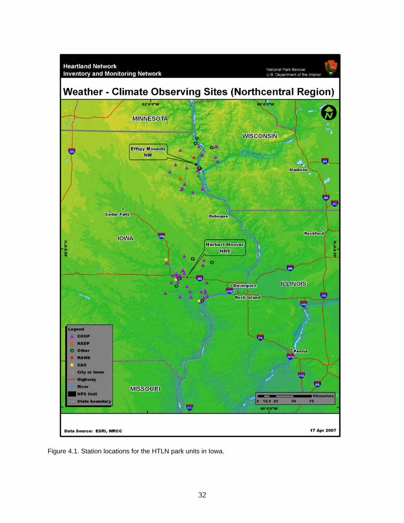
32

Figure 4.1. Station locations for the HTLN park units in Iowa.

33

February 1999. The COOP station at Iowa City Municipal Airport and its collocated SAO station have been active since 1933. The data records at these sites, which are 16 km west of HEHO, are both reliably complete. The COOP station “Muscatine” is 37 km southeast of HEHO and has a data record which goes back to 1935 and is very complete. The COOP station “Illinois City Dam 16,” which is 39 km southeast of HEHO, has been active since 1940. This site has had sporadic temperature measurements but its precipitation measurements have been largely complete except for a larger gap from May 1986 to October 1987. Besides the SAO network sites discussed above, several other weather networks provide near-real-time data within 40 km of HEHO. The AWDN station “Muscatine” has been operating since 2000 (Table 4.3) and is almost 40 km southeast of HEHO (Figure 4.1). Two CWOP stations have been identified within 40 km of HEHO, one at Hills (19 km southwest) and the other at Iowa City (11 km west). The UPR network also has stations in the area, one at Lowden and the other at Mechanicsville. 4.2.2. Kansas, Nebraska, and Minnesota No weather or climate stations were identified within HOME (Table 4.4). Of the 36 COOP stations we identified within 40 km of the boundaries of HOME, 12 are active. The closest active COOP station is “Beatrice 1 N” (1984-present), which is 6 km east of HOME. The longest records come from the COOP stations “Beatrice” and “Fairbury,” both of which have observations going back to January 1893. “Beatrice” is 7 km east of HOME, while “Fairbury” is 33 km southwest of HOME. The latter station has a very complete data record; however, “Beatrice” has been unreliable after 1984. The COOP station “Crete” is another COOP station with data going back to 1893 (July). This station is located 37 km north of HOME and has a very complete data record. The COOP station “Hickman” (1894-present) measures precipitation only and has had a reliable data record since 1948. The COOP station “Wymore” (1897-present), 22 km southeast of HOME, measures precipitation only and has had a reliable data record with the exception of a gap from June 1986 to February 1987. The COOP station “Western” (1910-present) is 32 km west of HOME and measures precipitation only. This site had numerous data gaps in the 1960s and 1970s. The COOP station “Virginia” is 28 km east of HOME and has been active since 1926. Precipitation measurements at this site have been largely complete, with only scattered, small data gaps. Temperature measurements have only been made since the late 1980s. Four different weather stations currently provide near-real-time data within 40 km of HOME (Table 4.4; Figure 4.2). The AWDN station “Beatrice” is located 8 km east of HOME and has been active since 1990. A CWOP station is present in the town of Crete, almost 40 km north of HOME. The UPR network has two stations in the area, one at Fairbury and the other at Rudy. Table 4.4. Weather and climate stations for the HTLN park units in Kansas, Nebraska, and Minnesota. Stations inside park units and within 40 km of the park unit boundary are included. Missing entries are indicated by “M”.

Name Lat. Lon. Elev. (m) Network Start End In Park?

Homestead National Monument of America (HOME) Beatrice 40.300 -96.933 376 AWDN 1/1/1990 Present No Barneston 40.049 -96.575 366 COOP 8/1/1950 8/1/2005 No Beatrice 40.250 -96.750 372 COOP 1/1/1893 Present No Beatrice 1 N 40.299 -96.750 395 COOP 11/1/1984 Present No

34

Name Lat. Lon. Elev. (m) Network Start End In Park?Beatrice 2 40.267 -96.733 400 COOP 8/1/1948 6/11/1979 No Beatrice KWBE 40.267 -96.783 397 COOP 11/1/1954 8/31/1973 No Crete 40.596 -96.959 415 COOP 6/1/1949 Present No Crete 40.619 -96.947 437 COOP 7/1/1893 Present No Crete 2 SE 40.617 -96.917 451 COOP 7/1/1956 6/30/1961 No Endicott 40.083 -97.133 M COOP 7/1/1936 2/28/1958 No Fairbury 40.136 -97.171 415 COOP 1/1/1893 Present No Fairbury #2 40.115 -97.170 420 COOP 7/15/2006 Present No Fairbury 2 SSE 40.117 -97.167 445 COOP 2/1/1958 12/31/1958 No Firth 40.535 -96.608 408 COOP 7/1/1921 11/15/2000 No Hallam 2 N 40.567 -96.783 442 COOP 8/1/1956 1/1/1996 No Hallam 3 W 40.533 -96.850 427 COOP 7/1/1956 6/30/1961 No Hickman 40.622 -96.628 396 COOP 11/1/1894 Present No Hickman 2 SW 40.583 -96.633 M COOP 11/1/1950 7/1/1972 No Hickman 2 WSW 40.600 -96.667 418 COOP 7/1/1956 6/30/1961 No Hickman 3 W 40.617 -96.667 387 COOP 7/1/1956 6/30/1961 No Holland 40.583 -96.583 412 COOP 7/1/1956 6/30/1961 No Jansen 3 NE 40.200 -97.033 445 COOP 4/1/1958 4/27/2000 No Kramer 40.583 -96.867 418 COOP 6/1/1948 7/19/1978 No Martell 5 W 40.617 -96.850 442 COOP 7/1/1956 6/30/1961 No Pickrell 1 W 40.383 -96.750 421 COOP 7/1/1956 9/30/1957 No Pickrell 2 NW 40.400 -96.750 439 COOP 7/1/1956 9/30/1957 No Princeton 40.567 -96.700 436 COOP 7/1/1956 6/30/1961 No Princeton 2 N 40.600 -96.700 418 COOP 7/1/1956 6/30/1961 No Princeton 2 NW 40.583 -96.733 439 COOP 7/1/1956 6/30/1961 No Princeton 3 N 40.617 -96.700 415 COOP 7/1/1956 6/30/1961 No Sprague 40.633 -96.733 381 COOP 8/6/1942 5/12/2000 No Sprague 1 ESE 40.617 -96.717 403 COOP 7/1/1956 6/30/1961 No Sprague 3 W 40.633 -96.783 396 COOP 2/14/1984 Present No Virginia 40.244 -96.498 471 COOP 3/1/1926 Present No Western 40.395 -97.193 451 COOP 2/1/1910 Present No Wilber 3 W 40.480 -97.012 406 COOP 8/8/1958 Present No Wymore 40.127 -96.671 383 COOP 12/1/1897 Present No CW4251 Crete 40.622 -96.952 420 CWOP M Present No Beatrice Muni. Arpt. 40.317 -96.750 397 SAO 2/1/1950 6/24/1993 No Fairbury 40.155 -97.200 402 UPR M Present No Rudy 40.042 -97.026 388 UPR M Present No

Pipestone National Monument (PIPE) Pipestone 44.014 -96.326 520 COOP 8/5/1877 Present Yes Airlie 44.000 -96.500 501 COOP 2/1/1894 9/30/1894 No Brookings 44.172 -96.749 473 COOP 5/1/1972 Present No Flandreau 44.052 -96.593 475 COOP 1/1/1893 Present No Garretson 43.717 -96.500 454 COOP 10/1/1950 2/27/1974 No Holland 44.083 -96.167 543 COOP 10/1/1892 6/30/1893 No Lake Wilson 43.998 -95.957 503 COOP 4/1/1973 Present No Luverne 43.666 -96.202 457 COOP 6/1/1893 Present No

35

Name Lat. Lon. Elev. (m) Network Start End In Park?Sioux Falls EROS Ctr. 43.738 -96.627 485 COOP 2/1/1974 Present No Slayton 9 SW 43.900 -95.883 482 COOP 7/1/1898 4/5/1973 No Tyler 44.278 -96.128 529 COOP 7/1/1916 Present No Sioux Falls 14 NNE 43.735 -96.622 486 CRN 9/25/2002 Present No CW2877 Luverne 43.653 -96.231 436 CWOP M Present No KC0OFZ Elkton 44.232 -96.480 533 CWOP M Present No Sioux Falls 43.730 -96.620 486 GPS-MET M Present No Pipestone Muni. Arpt. 43.983 -96.300 529 SAO 10/1/1990 Present No EROS Data Center 43.740 -96.610 488 SCAN M Present No

Tallgrass Prairie National Preserve (TAPR) Tallgrass Prairie NP 38.433 -96.558 381 COOP 12/1/1999 Present Yes Tallgrass Prairie 38.435 -96.561 399 RAWS 4/1/2002 Present Yes Americus 2 S 38.467 -96.250 338 COOP 11/1/1963 1/1/2004 No Burdick 38.567 -96.850 445 COOP 8/1/1951 6/30/1959 No Bushong 38.645 -96.351 424 COOP 3/1/1961 Present No Cedar Point 4 S 38.200 -96.833 384 COOP 5/1/1964 11/11/1981 No Cedar Point 4 S 38.199 -96.823 393 COOP 10/20/1997 8/20/2006 No Clements 38.300 -96.733 375 COOP 8/1/1966 10/1/1988 No Cottonwood Falls 38.369 -96.544 372 COOP 12/1/1902 Present No Cottonwood Falls ICT 38.367 -96.550 366 COOP 7/1/1956 11/30/1957 No Council Grove 38.667 -96.500 400 COOP 10/13/1908 10/31/1963 No Council Grove 38.650 -96.483 378 COOP M Present No Council Grove Lake 38.675 -96.526 402 COOP M Present No Council Grove Waterworks 38.667 -96.500 381 COOP 12/1/1956 4/30/1965 No Diamond Springs 5 W 38.566 -96.848 460 COOP 8/1/1948 Present No Dunlap 2 N 38.587 -96.391 357 COOP 3/1/1963 Present No Elk 38.417 -96.817 387 COOP 6/1/1959 4/30/1974 No Elmdale 38.367 -96.650 366 COOP 10/1/1932 6/30/1959 No Elmdale 38.413 -96.767 396 COOP 5/14/1975 Present No Elmdale 38.409 -96.618 363 COOP 2/14/1989 Present No Emporia 38.386 -96.182 328 COOP 1/1/1893 Present No Emporia 3 NW 38.429 -96.219 372 COOP M Present No Emporia Muni. Arpt. 38.331 -96.190 369 COOP 10/1/1950 Present No Florence 38.242 -96.924 393 COOP 10/1/1925 Present No Florence 3 E 38.236 -96.877 376 COOP 10/1/1963 Present No Gunter 5 S 38.375 -96.761 224 COOP 7/1/1947 5/1/2001 No Lincolnville 38.497 -96.962 433 COOP 8/1/1966 Present No Marion 38.350 -97.000 412 COOP 8/1/1948 4/10/1968 No Matfield Green 2 N 38.185 -96.569 396 COOP 5/1/1952 Present No Plymouth 1 SW 38.398 -96.356 338 COOP 11/1/1963 Present No Saffordville 38.391 -96.446 354 COOP 2/1/1962 2/26/1999 No Wilsey 38.632 -96.673 445 COOP 3/1/1961 Present No Wonsevu 38.111 -96.731 418 COOP 6/1/1959 Present No Emporia Muni. Arpt. 38.331 -96.190 369 SAO 10/1/1950 Present No Herington AAF 38.700 -96.817 455 WBAN 6/1/1943 9/30/1945 No

36

Figure 4.2. Station locations for the HTLN park units in Kansas, Nebraska, and Minnesota.

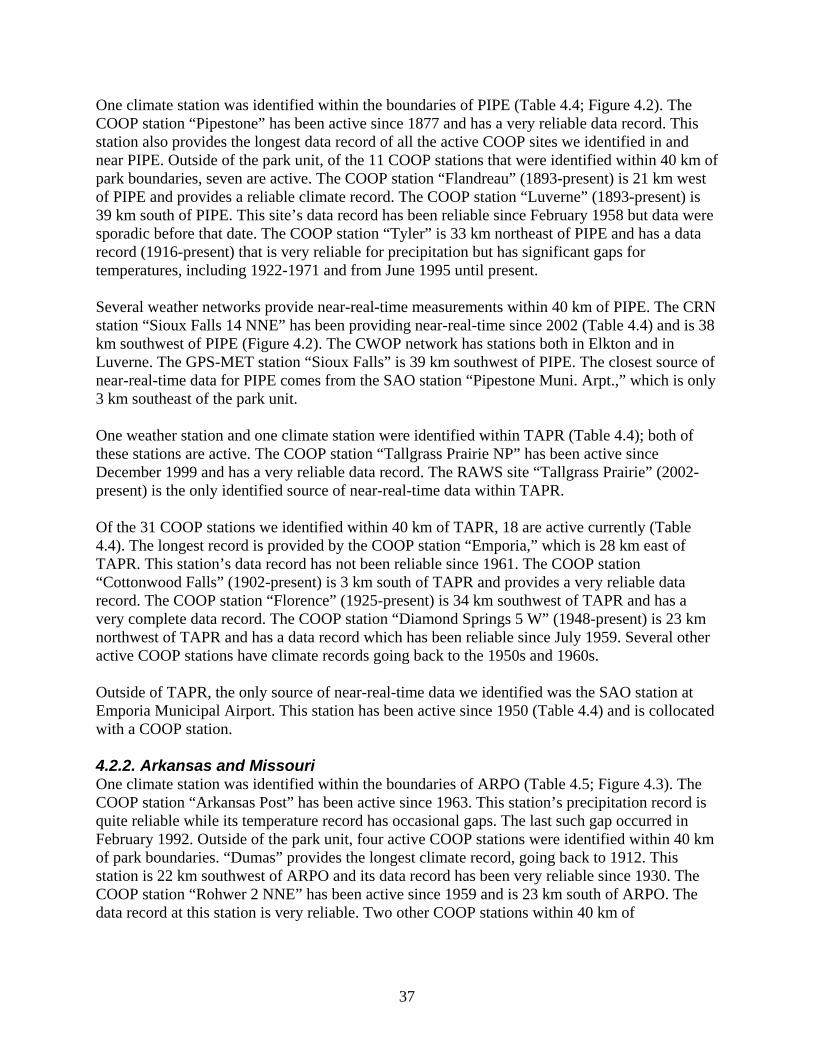
37

One climate station was identified within the boundaries of PIPE (Table 4.4; Figure 4.2). The COOP station “Pipestone” has been active since 1877 and has a very reliable data record. This station also provides the longest data record of all the active COOP sites we identified in and near PIPE. Outside of the park unit, of the 11 COOP stations that were identified within 40 km of park boundaries, seven are active. The COOP station “Flandreau” (1893-present) is 21 km west of PIPE and provides a reliable climate record. The COOP station “Luverne” (1893-present) is 39 km south of PIPE. This site’s data record has been reliable since February 1958 but data were sporadic before that date. The COOP station “Tyler” is 33 km northeast of PIPE and has a data record (1916-present) that is very reliable for precipitation but has significant gaps for temperatures, including 1922-1971 and from June 1995 until present. Several weather networks provide near-real-time measurements within 40 km of PIPE. The CRN station “Sioux Falls 14 NNE” has been providing near-real-time since 2002 (Table 4.4) and is 38 km southwest of PIPE (Figure 4.2). The CWOP network has stations both in Elkton and in Luverne. The GPS-MET station “Sioux Falls” is 39 km southwest of PIPE. The closest source of near-real-time data for PIPE comes from the SAO station “Pipestone Muni. Arpt.,” which is only 3 km southeast of the park unit. One weather station and one climate station were identified within TAPR (Table 4.4); both of these stations are active. The COOP station “Tallgrass Prairie NP” has been active since December 1999 and has a very reliable data record. The RAWS site “Tallgrass Prairie” (2002-present) is the only identified source of near-real-time data within TAPR. Of the 31 COOP stations we identified within 40 km of TAPR, 18 are active currently (Table 4.4). The longest record is provided by the COOP station “Emporia,” which is 28 km east of TAPR. This station’s data record has not been reliable since 1961. The COOP station “Cottonwood Falls” (1902-present) is 3 km south of TAPR and provides a very reliable data record. The COOP station “Florence” (1925-present) is 34 km southwest of TAPR and has a very complete data record. The COOP station “Diamond Springs 5 W” (1948-present) is 23 km northwest of TAPR and has a data record which has been reliable since July 1959. Several other active COOP stations have climate records going back to the 1950s and 1960s. Outside of TAPR, the only source of near-real-time data we identified was the SAO station at Emporia Municipal Airport. This station has been active since 1950 (Table 4.4) and is collocated with a COOP station. 4.2.2. Arkansas and Missouri One climate station was identified within the boundaries of ARPO (Table 4.5; Figure 4.3). The COOP station “Arkansas Post” has been active since 1963. This station’s precipitation record is quite reliable while its temperature record has occasional gaps. The last such gap occurred in February 1992. Outside of the park unit, four active COOP stations were identified within 40 km of park boundaries. “Dumas” provides the longest climate record, going back to 1912. This station is 22 km southwest of ARPO and its data record has been very reliable since 1930. The COOP station “Rohwer 2 NNE” has been active since 1959 and is 23 km south of ARPO. The data record at this station is very reliable. Two other COOP stations within 40 km of

38

Table 4.5. Weather and climate stations for the HTLN park units in Arkansas and Missouri. Stations inside park units and within 40 km of the park unit boundary are included. Missing entries are indicated by “M”.

Name Lat. Lon. Elev. (m) Network Start End In Park?

Arkansas Post National Monument (ARPO) Arkansas Post 34.025 -91.344 59 COOP 8/1/1963 Present Yes Arkansas Post 6 E LK2 34.033 -91.250 55 COOP 6/1/1967 5/1/1988 No Cummins Farm 34.067 -91.583 55 COOP 6/15/1944 5/5/1965 No Dumas 33.885 -91.532 50 COOP 5/1/1912 Present No Dumas 33.883 -91.500 52 COOP 7/1/1947 2/28/1961 No Kelso 33.770 -91.273 44 COOP 4/1/1985 Present No McArthur 33.687 -91.334 44 COOP 4/1/1985 Present No Pendleton 33.983 -91.383 49 COOP 11/7/1990 12/31/1991 No Pinchback 33.967 -91.717 55 COOP 7/1/1950 7/31/1960 No Rohwer 2 NNE 33.810 -91.270 46 COOP 12/1/1959 Present No Rosedale 33.850 -91.017 46 COOP 10/1/1894 6/30/1982 No Swan Lake 1 S 34.167 -91.700 52 COOP 12/1/1968 8/6/1982 No Watson 33.900 -91.267 45 COOP 11/1/1985 12/31/1988 No Yancopin 33.950 -91.217 52 COOP 12/1/1924 4/30/1938 No CW1630 DeWitt 34.300 -91.300 67 CWOP M Present No UAPB DeWitt 34.280 -91.350 60 SCAN M Present No

Buffalo National River (BUFF) St. Joe 35.984 -92.748 171 COOP 9/1/1970 11/5/2001 Yes Buffalo NR-Buffalo Point 36.084 -92.587 308 NADP 7/13/1982 Present Yes FRWS-12 Buffalo City 36.159 -92.459 274 RAWS 2/1/2003 11/30/2003 Yes Silver Hill 35.970 -92.746 283 RAWS 5/1/1998 Present Yes Berryville 36.360 -93.551 360 COOP 9/21/2001 Present No Big Flat 36.000 -92.400 381 COOP 12/21/1944 7/31/1960 No Botkinburg 3 NE 35.720 -92.471 395 COOP 6/1/1939 Present No Buffalo Tower 35.867 -93.500 786 COOP 8/1/1946 9/30/1987 No Bull Shoals Dam 36.365 -92.578 146 COOP 7/1/1947 Present No Calico Rock 2 36.116 -92.144 97 COOP 10/1/1984 Present No Calico Rock 2 WSW 36.109 -92.164 107 COOP 7/22/1904 Present No Canaan 2 W 35.867 -92.733 244 COOP 7/1/1947 10/31/1956 No Capps 36.233 -93.183 433 COOP 9/1/1970 4/9/1986 No Combs 35.800 -93.800 427 COOP 1/4/1946 9/30/1986 No Compton 36.092 -93.308 660 COOP 6/1/1939 Present No Cotter 36.283 -92.517 134 COOP 10/31/1927 2/28/1957 No Deer 35.827 -93.204 724 COOP 5/1/1975 Present No Denver 36.383 -93.300 314 COOP 7/1/1947 6/30/1955 No Devils Knob 35.717 -93.400 717 COOP 8/1/1937 6/7/1969 No Dutton 35.800 -93.700 485 COOP 4/1/1901 6/30/1937 No Flippin Arpt. 36.300 -92.583 215 COOP 6/1/1951 8/31/1979 No Gamaliel 36.415 -92.246 227 COOP 9/19/1989 Present No Gilbert 35.991 -92.715 189 COOP 7/1/1924 Present No Green Forest 36.339 -93.428 415 COOP 3/28/1940 10/18/2006 No Green Mtn. 36.033 -92.200 336 COOP 7/16/1937 10/31/1956 No

39

Name Lat. Lon. Elev. (m) Network Start End In Park?Harrison 36.196 -93.106 345 COOP 1/1/1892 Present No Harrison 6 S 36.144 -93.088 378 COOP 5/15/1986 Present No Harrison Boone Co. Arpt. 36.267 -93.157 419 COOP 8/15/1944 Present No Henderson 2 W 36.367 -92.267 177 COOP 9/12/1941 7/31/1960 No Hindsville 10 E 36.185 -93.687 456 COOP 4/1/2006 Present No Huntsville 36.083 -93.733 442 COOP 7/1/1894 10/1/1982 No Huntsville 1 SSW 36.070 -93.752 543 COOP 5/1/1983 Present No Iceledo 35.867 -92.983 415 COOP 7/1/1947 10/31/1950 No Jasper 36.001 -93.188 256 COOP 7/1/1947 Present No Kingston 36.120 -93.577 408 COOP 3/1/2006 Present No Kingston 2 S 36.009 -93.521 654 COOP 4/1/2006 Present No Lost Corner 35.567 -92.833 473 COOP 8/1/1946 5/31/1958 No Lurton 35.800 -93.067 610 COOP 8/1/1946 5/29/1975 No Marshall 35.916 -92.639 309 COOP 8/1/1946 Present No Maumee 36.050 -92.650 244 COOP 7/1/1947 1/13/1987 No Melbourne 5 W 36.082 -91.982 152 COOP 8/1/1946 Present No Mtn. Home 1 NNW 36.346 -92.394 244 COOP 3/1/1902 Present No Mtn. Home C. Of E. 36.333 -92.383 244 COOP 1/1/1953 2/28/1987 No Mtn. View 35.863 -92.085 240 COOP 6/10/1924 7/31/2006 No Norfork Dam 36.249 -92.256 130 COOP 8/1/1946 Present No Omaha 2 36.462 -93.192 396 COOP 9/20/1989 8/1/2000 No Ozone 35.645 -93.419 579 COOP 8/1/1890 Present No Parthenon 35.955 -93.242 274 COOP 3/12/1940 Present No Pelsor 35.717 -93.100 610 COOP 2/1/1962 1/1/1964 No Pettigrew 6 NE 35.881 -93.551 668 COOP 4/1/2006 Present No Pyatt 36.250 -92.850 244 COOP 7/1/1947 2/10/1970 No Rockhouse 36.283 -93.667 369 COOP 7/1/1947 5/31/1953 No Rudd 36.213 -93.485 442 COOP 9/20/1989 Present No St. Paul 35.824 -93.767 424 COOP 3/1/1988 Present No Turnpike 35.667 -93.083 637 COOP 1/1/1925 1/31/1961 No Yellville 2 SSE 36.200 -92.667 244 COOP 12/10/1944 3/31/1993 No CW4709 Capps 36.237 -93.197 451 CWOP M Present No Uppr Buffalo Riv./Deer 35.826 -93.203 727 DRI 6/1/2003 3/31/2005 No Devils Knob 35.611 -93.333 640 RAWS 3/1/1999 Present No Flippin Arpt. 36.300 -92.583 215 SAO 6/1/1951 8/31/1979 No Harrison Boone Co. Arpt. 36.267 -93.157 419 SAO 8/15/1944 Present No Mtn. Home Baxter Co. Regl. Arpt.

36.369 -92.470 283 SAO 10/22/1998 Present No

Deer 35.903 -93.255 562 WX4U M Present No Wayton Deer 35.904 -93.255 557 WX4U M Present No

George Washington Carver National Monument (GWCA) Diamond 2 W 36.986 -94.352 326 COOP 6/1/1973 Present Yes Anderson 36.652 -94.439 320 COOP 7/1/1943 Present No Anderson 36.650 -94.517 320 COOP M Present No Carthage 5 S 37.177 -94.305 298 COOP 3/1/1893 Present No Carthage River 37.183 -94.317 281 COOP 4/1/1967 5/31/1974 No

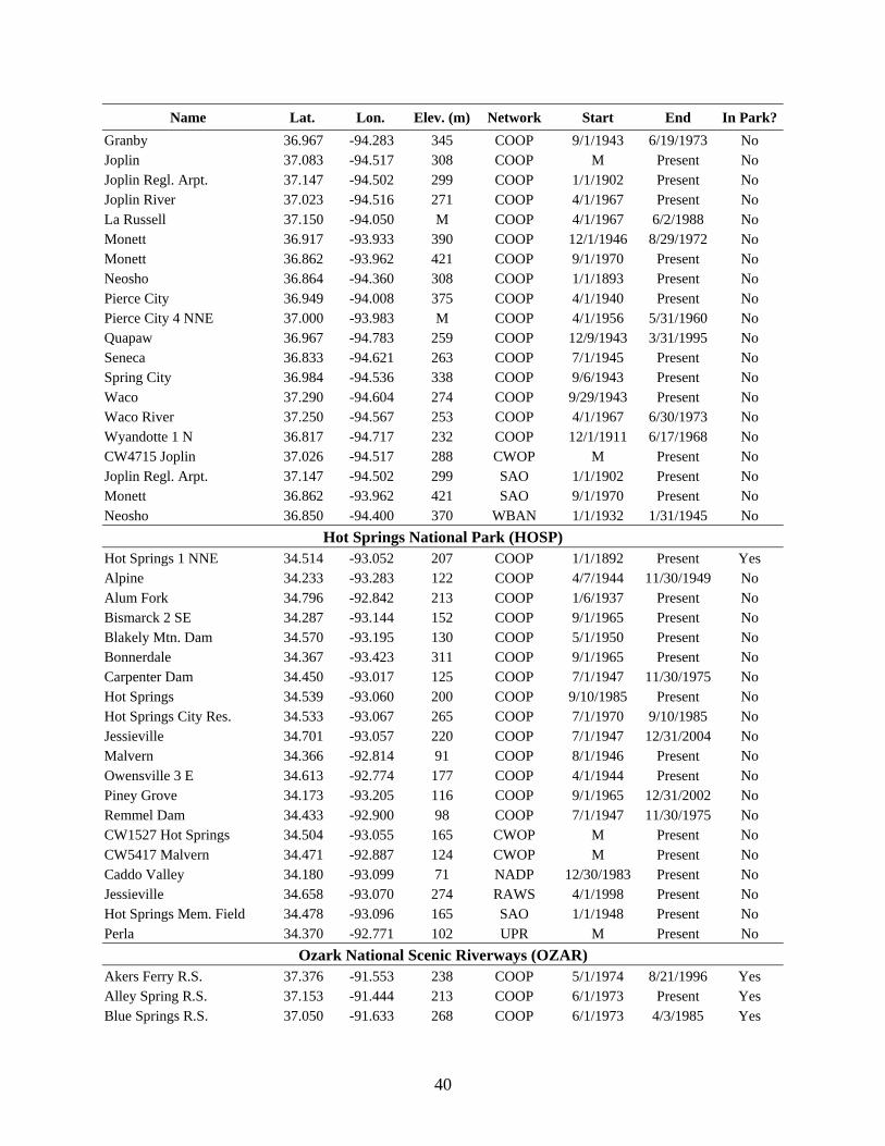
40

Name Lat. Lon. Elev. (m) Network Start End In Park?Granby 36.967 -94.283 345 COOP 9/1/1943 6/19/1973 No Joplin 37.083 -94.517 308 COOP M Present No Joplin Regl. Arpt. 37.147 -94.502 299 COOP 1/1/1902 Present No Joplin River 37.023 -94.516 271 COOP 4/1/1967 Present No La Russell 37.150 -94.050 M COOP 4/1/1967 6/2/1988 No Monett 36.917 -93.933 390 COOP 12/1/1946 8/29/1972 No Monett 36.862 -93.962 421 COOP 9/1/1970 Present No Neosho 36.864 -94.360 308 COOP 1/1/1893 Present No Pierce City 36.949 -94.008 375 COOP 4/1/1940 Present No Pierce City 4 NNE 37.000 -93.983 M COOP 4/1/1956 5/31/1960 No Quapaw 36.967 -94.783 259 COOP 12/9/1943 3/31/1995 No Seneca 36.833 -94.621 263 COOP 7/1/1945 Present No Spring City 36.984 -94.536 338 COOP 9/6/1943 Present No Waco 37.290 -94.604 274 COOP 9/29/1943 Present No Waco River 37.250 -94.567 253 COOP 4/1/1967 6/30/1973 No Wyandotte 1 N 36.817 -94.717 232 COOP 12/1/1911 6/17/1968 No CW4715 Joplin 37.026 -94.517 288 CWOP M Present No Joplin Regl. Arpt. 37.147 -94.502 299 SAO 1/1/1902 Present No Monett 36.862 -93.962 421 SAO 9/1/1970 Present No Neosho 36.850 -94.400 370 WBAN 1/1/1932 1/31/1945 No

Hot Springs National Park (HOSP) Hot Springs 1 NNE 34.514 -93.052 207 COOP 1/1/1892 Present Yes Alpine 34.233 -93.283 122 COOP 4/7/1944 11/30/1949 No Alum Fork 34.796 -92.842 213 COOP 1/6/1937 Present No Bismarck 2 SE 34.287 -93.144 152 COOP 9/1/1965 Present No Blakely Mtn. Dam 34.570 -93.195 130 COOP 5/1/1950 Present No Bonnerdale 34.367 -93.423 311 COOP 9/1/1965 Present No Carpenter Dam 34.450 -93.017 125 COOP 7/1/1947 11/30/1975 No Hot Springs 34.539 -93.060 200 COOP 9/10/1985 Present No Hot Springs City Res. 34.533 -93.067 265 COOP 7/1/1970 9/10/1985 No Jessieville 34.701 -93.057 220 COOP 7/1/1947 12/31/2004 No Malvern 34.366 -92.814 91 COOP 8/1/1946 Present No Owensville 3 E 34.613 -92.774 177 COOP 4/1/1944 Present No Piney Grove 34.173 -93.205 116 COOP 9/1/1965 12/31/2002 No Remmel Dam 34.433 -92.900 98 COOP 7/1/1947 11/30/1975 No CW1527 Hot Springs 34.504 -93.055 165 CWOP M Present No CW5417 Malvern 34.471 -92.887 124 CWOP M Present No Caddo Valley 34.180 -93.099 71 NADP 12/30/1983 Present No Jessieville 34.658 -93.070 274 RAWS 4/1/1998 Present No Hot Springs Mem. Field 34.478 -93.096 165 SAO 1/1/1948 Present No Perla 34.370 -92.771 102 UPR M Present No

Ozark National Scenic Riverways (OZAR) Akers Ferry R.S. 37.376 -91.553 238 COOP 5/1/1974 8/21/1996 Yes Alley Spring R.S. 37.153 -91.444 213 COOP 6/1/1973 Present Yes Blue Springs R.S. 37.050 -91.633 268 COOP 6/1/1973 4/3/1985 Yes

41

Name Lat. Lon. Elev. (m) Network Start End In Park?Eminence 10 E 37.184 -91.175 168 COOP 5/1/1988 8/22/1996 Yes Eminence 5 WNW 37.150 -91.450 214 COOP 1/4/1946 6/1/1973 Yes Eminence 8 NE 37.183 -91.250 183 COOP 6/1/1973 4/30/1979 Yes Pulltite R.S. 37.334 -91.489 232 COOP 8/1/1974 8/21/1996 Yes Alton 10 SE 36.633 -91.233 M COOP 8/1/1940 12/31/1948 No Alton 6 SE 36.630 -91.304 247 COOP 3/1/1940 Present No Annapolis 3 SW 37.300 -90.767 180 COOP 8/1/1923 7/25/1980 No Birch Tree 36.983 -91.500 305 COOP 8/1/1893 11/5/1968 No Bunker 37.514 -91.194 366 COOP 8/1/1923 Present No Cedar Grove R.S. 37.417 -91.600 290 COOP 5/1/1974 8/24/1979 No Centerville 37.437 -90.964 256 COOP 1/1/1893 3/1/1999 No Centerville R.S. 37.433 -90.950 M COOP 11/1/1936 9/30/1960 No Clearwater Dam 37.132 -90.776 201 COOP 11/1/1946 Present No Doniphan 36.621 -90.813 101 COOP 4/1/1904 Present No Doniphan 1 W 36.617 -90.850 98 COOP 7/1/1935 5/31/1973 No Eastwood Lookout 36.883 -91.033 293 COOP M Present No Ellington 37.233 -90.970 223 COOP 6/1/1939 Present No Ellsinore 36.933 -90.750 226 COOP 12/1/1940 5/17/1972 No Eminence 1 N 37.156 -91.359 195 COOP 6/1/1973 Present No Fremont Tower 36.967 -91.233 M COOP 6/1/1940 11/30/1960 No Greer 1 NE 36.750 -91.383 262 COOP 5/1/1974 10/1/1994 No High Lookout 36.883 -91.450 M COOP 6/1/1940 11/30/1950 No Houston 1 NE 37.341 -91.948 394 COOP 1/1/1893 Present No Houston 1 SE 37.317 -91.967 M COOP 1/1/1902 7/31/1955 No Houston 2 W 37.334 -92.006 328 COOP 6/1/1959 Present No Leeper 37.067 -90.700 M COOP 7/1/1948 4/30/1953 No Licking 4 N 37.554 -91.883 360 COOP 9/1/1936 Present No Licking 7 W 37.517 -91.983 278 COOP 6/1/1959 1/9/1994 No Macedonia Lookout 36.750 -90.900 M COOP 6/1/1940 2/28/1957 No Montauk S.P. 37.453 -91.683 283 COOP 6/1/1973 Present No Mtn. View 36.933 -91.783 314 COOP 9/1/1986 5/1/1996 No Mtn. View 5 W 36.991 -91.794 366 COOP 6/6/2001 Present No Oates Tower 37.533 -91.050 M COOP 10/5/1940 6/30/1951 No Reynolds 37.401 -91.079 378 COOP 7/20/1941 Present No Riverton 36.633 -91.200 165 COOP 5/1/1974 1/21/1992 No Round Spring 37.260 -91.428 249 COOP 2/20/1893 Present No Salem 37.633 -91.536 366 COOP 9/1/1903 Present No Summersville 37.178 -91.653 360 COOP 4/3/1940 Present No Thomasville 36.783 -91.533 195 COOP 5/1/1974 6/1/1994 No Tyrone 2 NNW 37.233 -91.883 403 COOP 9/1/1949 12/31/1977 No Van Buren 36.999 -91.011 151 COOP 2/1/1937 6/1/2006 No Van Buren R.S. 36.975 -91.019 305 COOP 8/1/1963 9/25/2001 No Victoria C P & L 37.633 -91.917 372 COOP 6/1/1973 10/1/1985 No West Plains 36.743 -91.835 308 COOP 2/1/1937 Present No White Church 36.901 -91.772 311 COOP 8/1/1974 Present No Williamsville 36.971 -90.559 155 COOP 2/1/1924 Present No

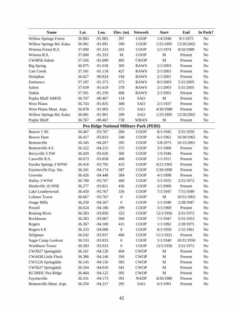
42

Name Lat. Lon. Elev. (m) Network Start End In Park?Willow Springs Forest 36.983 -91.983 397 COOP 1/4/1946 9/1/1973 No Willow Springs Rd. Kuku 36.981 -91.991 399 COOP 1/25/1895 12/20/2002 No Winona Forest R.S. 37.000 -91.333 265 COOP 5/1/1974 8/10/1989 No Winona R.S. 37.000 -91.333 M COOP M Present No CW4856 Salem 37.545 -91.699 405 CWOP M Present No Big Spring 36.975 -91.018 305 RAWS 2/1/2003 Present No Carr Creek 37.181 -91.118 427 RAWS 2/1/2001 Present No Doniphan 36.627 -90.824 194 RAWS 2/1/2001 Present No Eminence 37.187 -91.373 372 RAWS 8/1/2003 5/31/2005 No Salem 37.639 -91.619 378 RAWS 2/1/2003 5/31/2005 No Sinkin 37.501 -91.259 406 RAWS 2/1/2001 Present No Poplar Bluff AMOS 36.767 -90.467 114 SAO M Present No West Plains 36.743 -91.835 308 SAO 2/1/1937 Present No West Plains Muni. Arpt. 36.878 -91.903 373 SAO 4/30/1988 Present No Willow Springs Rd. Kuku 36.981 -91.991 399 SAO 1/25/1895 12/20/2002 No Poplar Bluff 36.767 -90.467 738 WBAN M Present No

Pea Ridge National Military Park (PERI) Beaver 1 SE 36.467 -93.767 284 COOP 8/1/1945 5/31/1959 No Beaver Dam 36.417 -93.833 348 COOP 6/1/1961 10/30/1965 No Bentonville 36.345 -94.207 395 COOP 5/8/1975 10/15/2001 No Bentonville 4 S 36.322 -94.215 372 COOP 3/1/1906 Present No Berryville 5 NW 36.429 -93.626 360 COOP 1/5/1946 Present No Cassville R.S. 36.673 -93.858 408 COOP 1/1/1911 Present No Eureka Springs 3 WNW 36.416 -93.792 433 COOP 4/21/1902 Present No Fayetteville Exp. Stn. 36.101 -94.174 387 COOP 5/20/1890 Present No Gravette 36.426 -94.448 384 COOP 4/1/1898 Present No Hailey 3 WSW 36.700 -93.767 400 COOP 5/1/1925 2/25/1972 No Hindsville 10 NNE 36.277 -93.821 436 COOP 3/1/2006 Present No Lake Leatherwood 36.450 -93.767 336 COOP 7/1/1947 7/31/1949 No Lohmer Tower 36.667 -93.767 0 COOP M 10/31/1963 No Osage Mills 36.250 -94.267 0 COOP 1/1/1940 2/28/1947 No Powell 36.624 -94.186 299 COOP 3/1/1969 Present No Roaring River 36.583 -93.850 323 COOP 12/1/1956 3/31/1972 No Rockhouse 36.283 -93.667 369 COOP 7/1/1947 5/31/1953 No Rogers 36.367 -94.100 415 COOP 1/1/1892 2/28/1975 No Rogers 6 E 36.333 -94.000 0 COOP 6/1/1959 1/31/1961 No Seligman 36.542 -93.937 466 COOP 11/1/1921 Present No Sugar Camp Lookout 36.533 -93.833 0 COOP 1/1/1940 10/31/1950 No Washburn Tower 36.583 -93.933 0 COOP 12/1/1956 3/31/1972 No CW3927 Springdale 36.161 -94.120 404 CWOP M Present No CW4438 Little Flock 36.386 -94.146 394 CWOP M Present No CW5126 Springdale 36.145 -94.150 383 CWOP M Present No CW5627 Springdale 36.164 -94.010 341 CWOP M Present No KC5RDU Pea Ridge 36.464 -94.122 395 CWOP M Present No Fayetteville 36.101 -94.173 391 NADP 4/20/1980 Present No Bentonville Muni. Arpt. 36.350 -94.217 395 SAO 6/1/1991 Present No

43

Name Lat. Lon. Elev. (m) Network Start End In Park?Fayetteville Springdale NWAR

36.283 -94.300 392 SAO 4/28/1999 Present No

Rogers Muni. Arpt. 36.372 -94.107 412 SAO 5/30/1991 Present No Springdale Muni. Arpt. 36.167 -94.117 414 SAO 7/1/1986 Present No

Wilson’s Creek National Battlefield (WICR) Wilson's Creek 37.117 -93.417 366 RAWS 2/1/2003 5/31/2005 Yes Ash Grove 4 S 37.261 -93.591 312 COOP 5/1/1962 Present No Billings 2 N 37.054 -93.575 406 COOP 5/1/1962 Present No Chadwick 36.933 -93.050 418 COOP 7/1/1948 9/30/1955 No Crane 36.900 -93.567 0 COOP M 3/31/1972 No Galena 36.804 -93.466 319 COOP 12/1/1898 Present No Halltown 5 NW 37.253 -93.728 360 COOP 5/1/1962 Present No Miller 1 E 37.215 -93.823 395 COOP 1/1/1951 Present No Oldfield 36.976 -93.024 378 COOP 10/1/1955 2/15/2005 No Ozark 37.019 -93.234 346 COOP 1/1/1946 Present No Rogersville 37.117 -93.050 0 COOP 11/1/1944 12/31/1977 No Springfield Regl. Arpt. 37.240 -93.390 384 COOP 1/1/1897 Present No Springfield WBO 37.200 -93.300 404 COOP 1/1/1888 12/31/1940 No CW1248 Battlefield 37.120 -93.366 390 CWOP M Present No CW1599 Willard 37.406 -93.424 351 CWOP M Present No CW1646 Republic 37.110 -93.466 399 CWOP M Present No CW2642 Ozark 37.005 -93.203 360 CWOP M Present No CW5071 Ozark 37.085 -93.236 386 CWOP M Present No WX2CHS Springfield 37.202 -93.357 388 CWOP M Present No WX6X Springfield 37.201 -93.267 409 CWOP M Present No Springfield Regl. Arpt. 37.240 -93.390 384 SAO 1/1/1897 Present No Springfield 37.200 -93.300 404 WBAN 1/1/1902 12/31/1947 No ARPO, “Kelso” and “McArthur,” have been operating since 1985. “McArthur” is 36 km south of ARPO, while “Kelso” is 27 km southeast of ARPO. Only two sources of near-real-time weather data were identified within 40 km of ARPO (Table 4.5; Figure 4.3). The CWOP station “CW1630 DeWitt” is 31 km north of ARPO and the SCAN station “UAPB DeWitt” is 28 km north of ARPO. Four weather and climate stations were identified within BUFF (Table 4.5). However, only two of these stations are active. These active stations are both located in eastern BUFF (Figure 4.3) and include the NADP station “Buffalo NR-Buffalo Point” (1982-present) and the RAWS site “Silver Hill” (1998-present). The COOP station “St. Joe” operated in central BUFF from 1970 until 2001 but is no longer active. Of the 52 COOP stations we identified within 40 km of BUFF, half of these (26) are active currently (Table 4.5). The closest active COOP station to BUFF is “Gilbert” (1924-present), which is less than a kilometer from the park unit and has a very complete data record. The

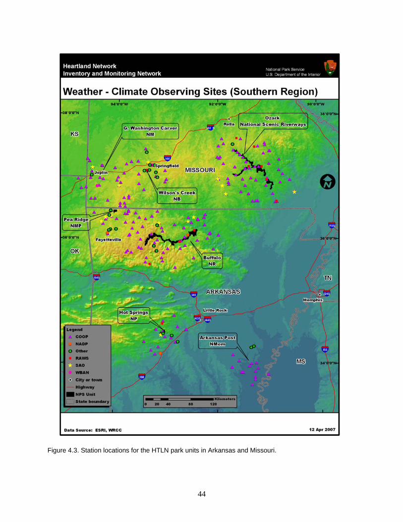
44

Figure 4.3. Station locations for the HTLN park units in Arkansas and Missouri.

45

longest record is provided by the COOP station “Ozone,” which is 29 km southwest of BUFF. This station’s data record has numerous, small gaps. The COOP station “Harrison,” 14 km north of BUFF, also provides a data record going back to the 1890s (1892-present). The data record at “Harrison” has some significant gaps, however. Temperature data have not been reliable since April 1975, while precipitation data, although measured currently, had a large gap from April 1975 to July 2001. The COOP station “Mtn. Home 1 NNW” is 19 km northeast of BUFF and has been active since 1902. This station’s data record is largely complete but there are scattered, small data gaps, particularly early on in the record (1940s and earlier). The COOP station “Calico Rock 2 WSW” is 22 km east of BUFF and has been active since 1904. Precipitation observations have been quite reliable at this site, while temperature observations show a gap from July 1937 to December 1963. Several other COOP stations within 40 km of BUFF have long climate records, going back to the1930s and 1940s. We identified one active RAWS site and two active SAO stations within 40 km of BUFF (Table 4.5; Figure 4.3). The RAWS site “Devils Knob” is located 34 km southwest of BUFF and has been active since 1999. This site has had numerous data gaps, including the latest gap in August 2004. The SAO station “Harrison Boone Co. Arpt.” is 19 km north of the western end of BUFF and has a data record going back to 1944. However, data from this site are unreliable. The SAO station “Mtn. Home Baxter Co. Regl. Arpt.” is 22 km northeast of BUFF and has a data record that is quite reliable and goes back to 1998. In addition to these stations, one CWOP station and two WX4U stations provide near-real-time weather data in the area. One station was identified within the boundaries of GWCA (Table 4.5; Figure 4.3). The COOP station “Diamond 2 W” has been active since 1973. This station’s precipitation record is largely complete except for a significant gap between February 1988 and September 1989. Temperature measurements have only been available at “Diamond 2 W” since February 1993. Outside of the park unit, of the 20 COOP stations that were identified within 40 km of park boundaries, 12 are active. “Neosho” provides the longest climate record, going back to 1893. This climate station is 13 km south of GWCA and its data record has been very reliable. The COOP station “Carthage 5 S,” 21 km north of GWCA, also has a data record that extends back to 1893 but its data record has not been reliable for the past 15 years. The COOP station “Joplin Regl. Arpt.” is 21 km northwest of GWCA and has a reliable data record that extends back to 1902. Five other COOP stations within 40 km of GWCA have been operating since the 1940s. We identified two active SAO stations within 40 km of GWCA (Table 4.5; Figure 4.3). “Joplin Regl. Arpt.” is 21 km northwest of GWCA, while “Monett” (1970-present) is 37 km east of GWCA. In addition to these near-real-time stations, one CWOP station was identified in Joplin, 14 km northwest of GWCA. One climate station was identified within the boundaries of HOSP (Table 4.5; Figure 4.3). The COOP station “Hot Springs 1 NNE” has been active since 1892 and has a very reliable data record. This station provides the longest data record of all the active COOP sites we identified in and near HOSP. Outside of the park unit, of the 13 COOP stations that were identified within 40 km of park boundaries, seven are active. The COOP station “Alum Fork” is 31 km northeast of HOSP and provides a reliable climate record that goes back to 1937. The COOP station “Owensville 3 E” is 24 km east of HOSP and has data going back to 1944. This site measures

46

precipitation only. Some gaps have occurred in the data record at “Owensville 3 E” during the 1990s and over the past 2-3 years. The COOP station “Malvern” is 26 km southeast of HOSP and has a data record (1946-present) that was very reliable up until the last 3 years. The COOP station “Blakely Mtn. Dam” is 10 km northwest of HOSP and has a data record (1950-present) that is quite complete except for no weekend measurements in the late 1980s. We identified one NADP site within 40 km of HOSP (Table 4.5; Figure 4.3). “Caddo Valley” is located 36 km south of HOSP and has been active since 1983. The primary source of near-real-time data outside of HOSP is the SAO station “Hot Springs Mem. Field,” which is 2 km southwest of HOSP (Figure 4.3) and has been operating since 1948 (Table 4.5). This station’s data record is quite reliable. The CWOP network has stations in Hot Springs and in Malvern (13 km east of HOSP). The RAWS station “Jessieville” is 11 km north of HOSP and has a reliable data record going back to 1998. The UPR network has a station at Perla. We identified seven COOP stations within OZAR (Table 4.5); however, only one of these is still active. This station is the COOP station “Alley Spring R.S.,” which has been active since 1973. Temperature measurements have not been reliable since June 1991; precipitation measurements, however, have been fairly reliable, with only scattered, small gaps in the record. Outside of OZAR, of the 46 COOP stations we identified within 40 km of the boundaries of OZAR, 20 are active. The longest record we identified was from the COOP station “Houston 1 NE,” which is 27 km west of OZAR and has been active since January 1893. This site had a significant data gap from 1926 to 1951 for precipitation and 1926 to 1960 for temperature. The COOP station “Round Spring” also has a data record going back to 1893. This station is only 2 km west of the central portion of OZAR. Temperatures have only been measured at this site within the past 7 years. The precipitation record is largely complete, with only scattered, small data gaps. The COOP station “Salem” (1903-present) is 21 km north of OZAR and has a reliable data record, as does the station “Doniphan” (1904-present), which is 24 km southeast of OZAR. The COOP station “Bunker” has been active since 1923 and is 30 km north of OZAR. Temperature measurements at “Bunker” have been most reliable since 1963 and precipitation measurements have been most reliable since 1948. This site has had numerous small gaps in its data record since 1990. The COOP station “Williamsville,” 30 km east of OZAR, has been active since 1924 and has a reliable data record. Several other COOP stations within 40 km of OZAR have data records extending back to the 1930s and 1940s. Four active RAWS stations were identified within 40 km of OZAR (Table 4.5). All of these stations have reliable data records. The RAWS stations “Big Spring” and “Carr Creek” are both less than a kilometer away from OZAR. “Doniphan” is 23 km southeast of OZAR and “Sinkin” is 25 km north of OZAR (Figure 4.3). Three active SAO stations were identified within 40 km of OZAR (Table 4.5). All of these stations have reliable data records. The closest SAO station to OZAR is “West Plains Muni. Arpt.,” which is 27 km southwest of the park unit (Figure 4.3). Of the two remaining active SAO stations, “West Plains” is 36 km southwest of OZAR and “Poplar Bluff Amos” is 40 km southeast of OZAR.

47

No weather or climate stations were identified within PERI (Table 4.5). Of the 22 COOP stations we identified within 40 km of the boundaries of PERI, nine are active. The closest active COOP station to PERI is “Seligman” (1921-present), which is 10 km northeast of the park unit. This site has numerous data gaps, with the most recent gap occurring from February 1990 to May 1994. The longest record comes from the COOP station “Fayetteville Exp. Stn.,” which has observations going back to 1890. This station is 37 km south of PERI. The data record at this site was quite complete until the last three years. The COOP station “Gravette” is another COOP station with data going back to the 1890s (1898). This station is located 34 km west of PERI and has a very reliable data record. The COOP station “Eureka Springs 3 WNW” (1902-present) is 19 km east of PERI and has a reliable data record except for no data during the month of October during the last two to three decades. The COOP station “Bentonville 4 S” is 18 km southwest of PERI and has data going back to 1906. This station has a very reliable data record. The COOP station “Cassville R.S.” (1911-present) is 26 km northeast of PERI. Temperature measurements at this station show a significant gap from 1920 to 1962, while precipitation measurements also show a gap, from 1920 to 1948. The COOP station “Berryville 5 NW” is 34 km east of PERI and measures precipitation only. This site has had a reliable data record (1946-present) except for a gap from October 1951 to June 1955. Several other networks have stations within 40 km of PERI. The NADP station “Fayetteville” has been operating since 1980, 37 km south of PERI. The closest source of near-real-time data for PERI comes from the CWOP station “KC5RDU Pea Ridge,” which is only 5 km west of the park unit. Four other active CWOP stations were identified for PERI, mostly in the community of Springdale. Four SAO stations were identified within 40 km of PERI (Table 4.5; Figure 4.3). The closest SAO station to PERI, “Rogers Muni. Arpt.” (1991-present), is located 6 km southwest of the park unit. Other SAO stations are located in the communities of Bentonville, Fayetteville, and Springdale. One station was identified within WICR (Table 4.5). This is a RAWS station (Wilson’s Creek) that is no longer active (2003-2005). Of the 12 COOP stations we identified within 40 km of WICR, seven are active currently (Table 4.5). The longest record is provided by the COOP station “Springfield Regl. Arpt.,” which is 14 km north of WICR. This station’s data record goes back to 1897 and is very reliable. A SAO station provides near-real-time data at this same location. The COOP station “Galena” (1898-present) is 31 km south of WICR. Temperatures were not measured at this site until 1963. The data record at “Galena” had a large data gap from 1903 to 1923. The COOP station “Ozark” is 16 km southeast of WICR and has data going back to 1946. This site, which measures precipitation only, has a data record that is largely complete except for scattered, small data gaps. Several other active COOP stations within 40 km of WICR have climate records going back to the 1950s and 1960s. Outside of WICR, the primary source of near-real-time data we identified is the aforementioned SAO station at Springfield Regional Airport. In addition to this station, seven active CWOP stations are located within 40 km of WICR (Table 4.5). The closest of these CWOP stations to WICR is “CW1248 Battlefield,” located only 3 km northeast of the park unit.

48

4.2.3. Indiana and Ohio We identified three weather and climate stations within CUVA (Table 4.6); however, only one of these is still active. This station is the COOP station “Old Portage,” which has been active since 1973 in southern CUVA. Unfortunately, the data record at “Old Portage” is unreliable. Outside of CUVA, of the 48 COOP stations we identified within 40 km of the boundaries of CUVA, 20 are active. The longest record we identified was from the COOP station “Hiram,” which is 30 km east of CUVA and has been active since 1893. This site has a very reliable data record. The COOP station “Chippewa Lake” is 31 km southwest of CUVA and has been active since 1895. This site has a very reliable data record. Three COOP stations we identified within 40 km of CUVA have reliable data records going back to 1896. The closest of these stations to CUVA is “Akron Fulton Intl. Arpt.,” 7 km south of the park unit. “Cleveland Hopkins Intl. Arpt.” is 17 km northwest of CUVA and “Elyria 3 E” is 33 km west of CUVA. Several other COOP stations within 40 km of CUVA have climate records going back to the1930s and 1940s. Table 4.6. Weather and climate stations for the HTLN park units in Indiana and Ohio. Stations inside park units and within 40 km of the park unit boundary are included. Missing entries are indicated by “M”.

Name Lat. Lon. Elev. (m) Network Start End In Park?

Cuyahoga Valley National Park (CUVA) Brecksville 3 N 41.367 -81.617 M COOP 6/1/1929 4/30/1948 Yes Old Portage 41.133 -81.550 226 COOP 10/1/1973 Present Yes Cuyahoga Valley 41.216 -81.581 300 GPMP 7/1/1985 1/31/1992 Yes Akron 41.157 -81.566 229 COOP 8/1/1948 Present No Akron 41.080 -81.517 329 COOP 1/1/1970 9/1/2000 No Akron Canton Regl. Arpt. 40.917 -81.433 368 COOP 7/1/1948 Present No Akron Fulton Intl. Arpt. 41.038 -81.464 318 COOP 5/1/1896 Present No Akron Steeles Corner 41.167 -81.517 317 COOP 12/1/1953 6/30/1967 No Alliance 40.933 -81.100 320 COOP 10/1/1926 10/31/1973 No Alliance 3 NNW 40.955 -81.117 322 COOP 8/1/1948 Present No Apco Ravenna Arsenal 41.167 -81.083 305 COOP 1/1/1948 8/31/1975 No Atwater Ctr. 41.017 -81.167 345 COOP 5/1/1894 6/30/1974 No Avon Lake 41.500 -82.033 183 COOP 2/1/1961 12/19/1986 No Burton 1 W 41.467 -81.167 354 COOP 7/28/1939 10/15/1993 No Canton 5 N 40.867 -81.400 345 COOP 5/1/1896 9/30/1948 No Canton Hwy. Dept. 40.767 -81.383 311 COOP 8/1/1948 2/29/1988 No Canton Repository 40.800 -81.383 320 COOP 12/1/1952 6/12/1970 No Chardon 41.583 -81.183 344 COOP 6/1/1945 Present No Charlestown 41.167 -81.150 360 COOP 7/1/1926 10/31/1938 No Chippewa Lake 41.052 -81.936 360 COOP 1/1/1895 Present No Chippewa Lake Waterworks 41.067 -81.900 317 COOP 8/1/1948 5/31/1951 No Cleveland Carroll Univ. 41.483 -81.700 230 COOP 1/1/1897 12/31/1930 No Cleveland Crib 41.550 -81.750 175 COOP 7/1/1950 Present No Cleveland Easterly 41.567 -81.583 168 COOP 8/1/1955 Present No Cleveland Hopkins Intl. Arpt.

41.405 -81.853 235 COOP 5/1/1896 Present No

Cleveland Lutheran M. 41.483 -81.717 210 COOP 5/11/1971 5/31/1978 No Cleveland Seven Hill 41.367 -81.667 351 COOP 1/1/1948 6/30/1950 No Cleveland Shaker Hts. 41.467 -81.567 299 COOP 1/1/1901 12/31/1953 No

49

Name Lat. Lon. Elev. (m) Network Start End In Park?Cleveland WB City 41.500 -81.667 201 COOP 6/1/1888 11/12/1957 No Doylestown Gas Co. 40.933 -81.700 305 COOP M 4/30/1955 No Elyria 3 E 41.383 -82.050 223 COOP 5/1/1896 Present No Elyria 4 S 41.300 -82.117 235 COOP 7/1/1971 Present No Garfield Hts. 41.417 -81.600 284 COOP 5/1/1971 5/31/1978 No Hiram 41.300 -81.150 375 COOP 6/1/1893 Present No Independence Teemark 41.400 -81.633 178 COOP 5/1/1966 Present No Kirtland-Holden 41.617 -81.300 228 COOP 12/1/1983 7/21/1994 No Kirtland-Holden 2 41.617 -81.300 314 COOP 7/21/1994 Present No Lagrange 1 NE 41.250 -82.100 249 COOP 7/1/1971 Present No Louisville 40.833 -81.250 357 COOP 3/15/1946 Present No Maple Hts. 41.400 -81.550 M COOP 7/1/1942 7/20/1955 No Marshallville 1 SSW 40.883 -81.733 341 COOP 3/1/1946 Present No Massillon 40.767 -81.533 283 COOP 2/1/1938 Present No Maximo 40.883 -81.183 360 COOP 7/1/1948 6/30/1974 No Parma Kyw. Transmitter 41.283 -81.617 329 COOP 6/1/1959 6/30/1961 No Ravenna 2 S 41.133 -81.283 337 COOP 8/1/1948 Present No Ravenna Pump Stn. 41.133 -81.233 329 COOP 7/1/1948 1/31/1949 No Stow 41.131 -81.404 323 COOP 1/1/1996 Present No Twinsburg 41.350 -81.500 345 COOP M 12/31/1975 No Willoughby 41.683 -81.383 192 COOP 7/1/1948 5/31/1953 No Willowghby East Lake 41.667 -81.433 195 COOP 7/2/1894 1/1/1977 No Willowghby River 41.633 -81.400 180 COOP 10/1/1973 2/17/1988 No AA3H Avon 41.392 -82.022 230 CWOP M Present No CW0221 Cleveland 41.423 -81.917 236 CWOP M Present No CW0393 Randolph 41.031 -81.447 348 CWOP M Present No CW1398 Akron 41.108 -81.511 336 CWOP M Present No CW2334 Moreland Hills 41.443 -81.443 334 CWOP M Present No CW2461 Fairview Park 41.443 -81.867 241 CWOP M Present No CW2494 Avon Lake 41.513 -82.013 184 CWOP M Present No CW2812 Brunswick 41.200 -81.800 325 CWOP M Present No CW3230 Middleburg Hts. 41.361 -81.812 259 CWOP M Present No CW4101 Medina 41.100 -81.750 300 CWOP M Present No CW4558 Cleveland 41.412 -81.742 259 CWOP M Present No CW4629 Kent 41.128 -81.364 329 CWOP M Present No CW5122 Sheffield Lake 41.487 -82.108 184 CWOP M Present No KA8OAD-1 Fairlawn 41.135 -81.604 305 CWOP M Present No KB8ROP Chardon 41.538 -81.180 354 CWOP M Present No KC8YFO Strongsville 41.343 -81.794 283 CWOP M Present No KF4IEQ Wondrely 41.656 -81.452 189 CWOP M Present No KG8QC North Olmsted 41.407 -81.932 237 CWOP M Present No N8FGR Orange 41.442 -81.464 365 CWOP M Present No N8VHJ Bedford 41.392 -81.516 296 CWOP M Present No WD8BMP-4 Copley 41.129 -81.647 328 CWOP M Present No Akron Canton Regl. Arpt. 40.917 -81.433 368 SAO 7/1/1948 Present No Akron Fulton Intl. Arpt. 41.038 -81.464 318 SAO 5/1/1896 Present No

50

Name Lat. Lon. Elev. (m) Network Start End In Park?Cleveland Burke Lakefront Arpt.

41.518 -81.684 178 SAO 1/1/1962 Present No

Cleveland Cuyahoga Co. Arpt.

41.567 -81.483 268 SAO 9/1/1962 Present No

Cleveland Hopkins Intl. Arpt.

41.405 -81.853 235 SAO 5/1/1896 Present No

Cleveland Lightboat 41.500 -81.717 184 SAO 5/1/1951 Present No Willoughby 41.683 -81.400 198 SAO 3/1/1971 Present No Wooster Wayne Co. Arpt. 40.873 -81.887 347 SAO 12/11/1996 Present No Akron NAS 41.033 -81.483 323 WBAN 1/1/1952 11/30/1957 No Chardon 41.580 -81.210 336 WX4U M Present No

Hopewell Culture National Historical Park (HOCU) Chillicothe Mound City 39.374 -83.004 198 COOP M Present Yes Chillicothe 39.386 -82.985 192 RAWS 9/1/2002 Present Yes Deer Creek State Park 39.636 -83.261 267 CASTNet 9/1/1988 Present No Alma Scioto Trails F. 39.217 -82.967 M COOP 8/1/1948 9/30/1949 No Bourneville 1 SSW 39.267 -83.167 215 COOP 6/1/1949 9/1/1986 No Chillicothe 39.333 -82.967 189 COOP 11/1/1897 1/28/1987 No Circleville 39.611 -82.955 205 COOP 11/15/1894 Present No Circleville 1 SW 39.576 -82.982 195 COOP 9/1/1990 Present No Deer Creek 39.625 -83.213 262 COOP 5/1/1968 Present No Greenfield 1 WNW 39.354 -83.406 296 COOP 1/1/1893 4/1/2005 No Hillsboro 39.200 -83.617 335 COOP 1/1/1893 Present No Hillsboro Water Work 39.233 -83.617 287 COOP 8/1/1948 5/31/1964 No Jackson 39.078 -82.705 244 COOP 3/25/1914 Present No Jackson Hwy. Dept. 39.050 -82.650 214 COOP 8/1/1948 6/30/1960 No Laurelville 39.467 -82.733 232 COOP 9/1/1951 Present No McArthur Hwy. Dept. 39.250 -82.467 235 COOP 8/1/1948 9/30/1957 No McArthur 39.250 -82.483 226 COOP 5/1/1893 2/1/1946 No McArthur 39.250 -82.482 239 COOP 5/1/1896 Present No Peebles 38.950 -83.417 247 COOP 1/1/1940 6/1/1985 No Peebles 1 S 38.933 -83.417 253 COOP 10/1/1910 8/31/1962 No Peebles 2 38.950 -83.400 240 COOP 9/1/1980 1/14/1985 No Piketon 39.071 -83.020 174 COOP 7/1/1942 Present No Piketon Water Works 39.068 -83.021 176 COOP 10/24/1985 1/1/2006 No Portsmouth Area WB 39.000 -83.000 204 COOP 7/1/1953 7/31/1955 No Washington Court House 39.527 -83.428 293 COOP 1/1/1915 9/1/2000 No Waverly 39.111 -82.980 171 COOP 6/1/1893 Present No Williamsport 39.583 -83.117 235 COOP M 12/7/1981 No CW4939 Peebles 38.949 -83.397 253 CWOP M Present No W8CTC Hillsboro 39.206 -83.599 338 CWOP M Present No Pikton 39.050 -83.020 176 GPS-MET M Present No Deer Creek State Park 39.636 -83.260 267 NADP 1/26/1999 Present No Piketon Water Works 39.068 -83.021 176 SAO 10/24/1985 1/1/2006 No Chillicothe 39.417 -82.900 267 WBAN 9/1/1941 12/31/1943 No Peebles 38.950 -83.383 259 WBAN 1/1/1937 4/30/1937 No

51

Name Lat. Lon. Elev. (m) Network Start End In Park?

Lincoln Boyhood National Monument (LIBO) Boonville 1 S 38.030 -87.274 122 COOP 10/1/1897 Present No Cannelton 37.899 -86.707 123 COOP 8/1/1971 Present No Ensor 37.800 -86.983 M COOP 2/1/1897 8/31/1899 No Ferdinand State Forest 38.250 -86.783 M COOP 7/1/1948 11/9/1957 No Grandview 37.954 -86.986 124 COOP 10/1/2001 Present No Hatfield 37.901 -87.230 119 COOP 3/1/1994 10/1/2000 No Holland 38.250 -87.033 M COOP 6/1/1902 11/30/1907 No Huntingburg 38.300 -86.967 154 COOP 3/1/1993 8/31/1996 No Huntingburg Arpt. 38.267 -86.950 159 COOP 2/1/1887 10/31/1957 No Jasper 38.386 -86.941 140 COOP 3/1/1893 Present No Jasper Radio WITZ 38.350 -86.933 140 COOP 6/1/1958 11/30/1960 No Lewisport 37.886 -86.910 128 COOP 6/1/1996 Present No Lynnville 3 N 38.250 -87.300 165 COOP 12/5/1947 12/9/1976 No Marchand Tower 38.100 -86.600 M COOP 2/1/1953 Present No Newburgh L & D 37.933 -87.374 116 COOP 1/1/1928 Present No Owensboro 37.783 -87.118 121 COOP 7/1/1896 10/1/2004 No Owensboro 3 E 37.791 -87.066 122 COOP 4/12/1960 Present No Owensboro Dam 46 L G 37.783 -87.133 M COOP 6/1/1948 12/31/1948 No Owensboro Treatment Plant 37.767 -87.083 125 COOP 1/1/1928 8/31/1990 No Rockport 4 N 37.939 -87.059 125 COOP 6/1/1992 9/13/2001 No Saint Meinrad 38.164 -86.809 155 COOP 4/1/1958 Present No Spurgeon 38.250 -87.250 152 COOP 3/1/1962 4/22/1995 No Stendal 38.269 -87.163 194 COOP 10/1/1995 Present No Tell City 37.953 -86.775 122 COOP 1/1/1902 Present No CW1123 Newburgh 37.976 -87.427 122 CWOP M Present No KB9LHX-6 Jasper 38.392 -86.930 153 CWOP M Present No KD9JB Oakland City 38.339 -87.354 145 CWOP M Present No N9LYA-1 Jasper 38.391 -86.931 152 CWOP M Present No Huntingburg Arpt. 38.249 -86.954 161 SAO 7/2/1993 Present No Tell City 37.953 -86.775 122 SAO 1/1/1902 Present No The primary sources of near-real-time weather data for CUVA are SAO sites. Eight active SAO stations are currently located within 40 km of CUVA (Table 4.6). The longest records (both going back to 1896) come from the SAO stations at the international airports in Akron and Cleveland. Other SAO stations providing reliable near-real-time data include “Akron Canton Regl. Arpt.” (20 km south of CUVA; Figure 4.4), “Cleveland Burke Lakefront Arpt.” (11 km northwest of CUVA), and “Wooster Wayne Co. Arpt.” (40 km southwest of CUVA). Numerous CWOP stations that provide near-real-time weather data have also been identified within 40 km of CUVA. Two stations were identified within HOCU (Table 4.6); both of these stations are active. The COOP station “Chillicothe Mound City” has been active since April 1972 and has a very reliable

52

Figure 4.4. Station locations for the HTLN park units in Indiana and Ohio.

53

a very reliable data record. The RAWS site “Chillicothe” (2002-present) is the only identified source of near-real-time data within HOCU. Of the 24 COOP stations we identified within 40 km of HOCU, nine of these are active currently (Table 4.6). The longest record is provided by the COOP station “Hillsboro,” which is 34 km southwest of HOCU. This station’s data record is very complete. Unfortunately, an active long-term record was lost within the past two years with the closing of the COOP station “Greenfield 1 WNW.” This station ceased taking measurements in April 2005. The COOP station “Waverly,” 20 km south of HOCU, also provides a data record going back to 1893. The data record at “Waverly” is very complete. The COOP station “Circleville” (1894-present) is 25 km north of HOCU and has a very complete data record. The COOP station “McArthur” (1896-present) is 37 km east of HOCU. Measurements at this site were sporadic before 1957. After 1957, the data record at “McArthur” has been very complete for precipitation. The COOP station “Jackson” is 30 km southeast of HOCU and has been active since 1914. The data record at this site has been reliable except for a large gap from August 1991 to September 1995. A few other active COOP stations have climate records going back to the1940s and 1950s. We identified one NADP site within 40 km of HOCU (Table 4.6; Figure 4.4). “Deer Creek State Park” is located 33 km northwest of HOCU and has been active since 1999. Several networks provide near-real-time data within 40 km of HOCU. The CASTNet station “Deer Creek State Park” is located 33 km northwest of HOCU (Figure 4.4) and has been active since 1988 (Table 4.6). The GPS-MET station “Piketon” is 28 km south of HOCU. The SAO station “Piketon Water Works” is 26 km south of HOCU but recently (January 2006) stopped taking measurements. Two CWOP stations have been identified, one in Peebles (35 km southwest of HOCU) and the other in Hillsboro (32 km southwest of HOCU). No weather or climate stations were identified within LIBO (Table 4.6). Of the 24 COOP stations we identified within 40 km of the boundaries of LIBO, 11 are active. The closest active COOP station to LIBO is “Saint Meinrad” (1958-present), which is 17 km east of the park unit and has a reliable data record. The longest record comes from the COOP station “Jasper,” which has observations going back to 1893. This climate station is 29 km north of LIBO. The COOP station “Boonville 1 S” is another COOP station with data going back to the 1890s (1897). This station is located 26 km southwest of LIBO. Precipitation measurements at “Boonville 1 S” have been largely complete, with only scattered, small data gaps, while temperature measurements have only been reliable since September 1990. The COOP station “Tell City” (1902-present) is 26 km southeast of LIBO and has a reliable data record. A SAO station is also located at this site. The COOP station “Newburgh L & D” is 38 km southwest of LIBO and measures precipitation only. This site has had a reliable data record (1928-present). A few other active COOP stations have records going back to the 1950s and earlier Two SAO stations were identified within 40 km of LIBO (Table 4.6; Figure 4.4). Besides the previously discussed SAO station at Tell City, “Huntingburg Arpt.” is located 14 km north of LIBO and provides the closest near-real-time measurements for LIBO. This station has been active since 1993. Four CWOP stations have been identified within 40 km of LIBO. The closest CWOP station is in Jasper, 30 km north of LIBO.

54

5.0. Conclusions and Recommendations We have based our findings on an examination of available climate records within HTLN units, discussions with NPS staff and other collaborators, and prior knowledge of the area. Here, we offer an evaluation and general comments pertaining to the status, prospects, and needs for climate-monitoring capabilities in the HTLN. The HTLN has already done much work inventorying weather and climate stations in its network and has established, in partnership with staff at the University of Missouri, data feeds from weather stations near several of its park units. 5.1. Heartland Inventory and Monitoring Network The HTLN network is committed to improving the weather- and climate-monitoring activities within their park units. At this point, we recall the primary objective of climate- and weather-monitoring activities in HTLN (DeBacker et al. 2005):

• Determine how climatic factors affecting plant and animal populations, communities, and

aquatic systems vary seasonally and annually. The current weather station data feed that has been established by HTLN is being utilized to meet this objective. Reliable long-term climate records are usually available either in HTLN park units or within 40 km of these park units, so this objective can likely be met by using data from these stations. Few near-real-time weather and climate stations were identified within the park units themselves. This is particularly critical for BUFF and OZAR. The only near-real-time stations we identified in BUFF are located in the eastern part of the park unit. There are no near-real-time weather stations in OZAR currently. Both BUFF and OZAR protect riverways that provide opportunities for setting up local climate transect measurements. Such transects would help to document spatial variations of extreme weather events and the associated disturbances that impact these relatively-pristine riverways. At BUFF, for instance, a RAWS installation in the western portion of the park unit would complement the existing RAWS sites in eastern BUFF. As an additional strategy for documenting the spatial characteristics of extreme weather and climate events in the HTLN, The NPS could encourage greater coverage of near-real-time weather stations outside of HTLN park units. The AWDN, RAWS, and SCAN networks each have a presence in the HTLN region and NPS could work with agencies such as the High Plains Regional Climate Center (HPRCC) for AWDN and NRCS for the SCAN network to encourage new weather station installations in or near HTLN park units. 5.2. Spatial Variations in Mean Climate With local variations over short horizontal distances, land use and irrigation can introduce considerable fine-scale structure to mean climate (temperature and precipitation) around some HTLN park units. Low-relief drainages within HTLN park units such as BUFF and OZAR can display significant nighttime temperature variations that are often undersampled by current surface weather and climate station networks. Convective summer precipitation events introduce a high level of spatial variability to precipitation characteristics in HTLN park units. Issues

55

encountered in mapping mean climate are discussed in Appendix D and in Redmond et al. (2005). For areas where new stations will be installed, if only a few new stations will be emplaced, the primary goal should be overall characterization of the main climate elements (temperature and precipitation and their joint relative, snow). This level of characterization generally requires that (a) stations should not be located in deep valley bottoms (cold air drainage pockets) or near excessively steep slopes and (b) stations should be distributed spatially in the major biomes of each park. If such stations already are present in the vicinity, then additional stations would be best used for two important and somewhat competing purposes: (a) add redundancy as backup for loss of data from current stations (or loss of the physical stations) or (b) provide added information on spatial heterogeneity in climate arising from topographic and land-use diversity. 5.3. Climate Change Detection There is much interest in the adaptation of HTLN ecosystems in response to possible future climate change. In particular, in light of the extensive land-use fragmentation which has taken place across the HTLN network, there are concerns about habitat shifts and abilities of plant and animal communities to migrate in response to climate changes (DeBacker et al. 2005). The desire for credible, accurate, complete, and long-term climate records—from any location—cannot be overemphasized. Thus, this consideration always should have a high priority. However, because of spatial diversity in climate, monitoring that fills knowledge gaps and provides information on long-term temporal variability in short-distance relationships also will be valuable. We cannot be sure that climate variability and climate change will affect all parts of a given park unit equally. In fact, it is appropriate to speculate that this is not the case, and spatial variations in temporal variability extend to small spatial scales, a consequence of diversity within HTLN in land use patterns. 5.4. Aesthetics This issue arises frequently enough to deserve comment. Standards for quality climate measurements require open exposures away from heat sources, buildings, pavement, close vegetation and tall trees, and human intrusion (thus away from property lines). By their nature, sites that meet these standards are usually quite visible. In many settings (such as heavily forested areas) these sites also are quite rare, making them precisely the same places that managers wish to protect from aesthetic intrusion. The most suitable and scientifically defensible sites frequently are rejected as candidate locations for weather and climate stations. Most weather and climate stations, therefore, tend to be “hidden” but many of these hidden locations have inferior exposures. Some measure of compromise is nearly always called for in siting weather and climate stations. The public has vast interest and curiosity in weather and climate, and within the NPS I&M networks, such measurements consistently rate near or at the top of desired public information. There seem to be many possible opportunities for exploiting and embracing this widespread interest within the interpretive mission of the NPS. One way to do this would be to highlight rather than hide these stations and educate the public about the need for adequate siting. A

56

number of weather displays we have encountered during visits have proven inadvertently to serve as counterexamples for how measurements should not be made. 5.5. Information Access Access to information promotes its use, which in turn promotes attention to station care and maintenance, better data, and more use. An end-to-end view that extends from sensing to decision support is far preferable to isolated and disconnected activities and aids the support infrastructure that is ultimately so necessary for successful, long-term climate monitoring. Decisions about improvements in monitoring capacity are facilitated greatly by the ability to examine available climate information. Various methods are being created at WRCC to improve access to that information. Web pages providing historic and ongoing climate data, and information from HTLN park units, can be accessed at http://www.wrcc.dri.edu/nps. In the event that this URL changes, there still will be links from the main WRCC Web page entitled “Projects” under NPS. The WRCC has been steadily developing software to summarize data from hourly sites. This has been occurring under the aegis of the RAWS program and a growing array of product generators ranging from daily and monthly data lists to wind roses and hourly frequency distributions. All park data are available to park personnel via an access code (needed only for data listings) that can be acquired by request. The WRCC RAWS Web page is located at http://www.wrcc.dri.edu/wraws or http://www.raws.dri.edu. Web pages have been developed to provide access not only to historic and ongoing climate data and information from HTLN park units but also to climate-monitoring efforts for HTLN. These pages can be found through http://www.wrcc.dri.edu/nps. Additional access to more standard climate information is accessible though the previously mentioned Web pages, as well as through http://www.wrcc.dri.edu/summary. These summaries are generally for COOP stations. 5.6. Summarized Conclusions and Recommendations

• HTLN has already recognized the importance of improving weather and climate station coverage within its park units (DeBacker et al. 2005) and is actively ingesting data from select weather stations near HTLN park units.

• The presence of reliable, long-term climate records near most HTLN park units is helpful for monitoring climate variations at longer time scales and their impacts on HTLN ecosystems.

• The ability to sample extreme weather events in the HTLN is currently restricted due to the lack of near-real-time stations within HTLN park units, especially BUFF and OZAR. Climate transects may be useful at both of these park units.

• NPS could facilitate expansion of near-real-time weather networks, such as AWDN, RAWS, and SCAN, by encouraging local and federal agencies to install additional stations near HTLN park units.

57

6.0 Literature Cited American Association of State Climatologists. 1985. Heights and exposure standards for sensors

on automated weather stations. The State Climatologist 9. Bevis, M., S. Businger, T. A. Herring, C. Rocken, R. A. Anthes, and R. H. Ware. 1992. GPS

meteorology: remote sensing of the atmospheric water vapor using the global positioning system. Journal of Geophysical Research 97:75–94.

Bonan, G. B. 2002. Ecological Climatology: Concepts and Applications. Cambridge University

Press. Bunkers, M. J., J. R. Miller, Jr., and A. T. DeGaetano. 1996. An examination of El Niño-La Niña

related precipitation and temperature anomalies across the Northern Plains. Journal of Climate 9:147-160.

Bureau of Land Management. 1997. Remote Automatic Weather Station (RAWS) and Remote

Environmental Monitoring Systems (REMS) standards. RAWS/REMS Support Facility, Boise, Idaho.

Chapin III, F. S., M. S. Torn, and M. Tateno. 1996. Principles of ecosystem sustainability. The

American Naturalist 148:1016-1037. Daly, C., R. P. Neilson, and D. L. Phillips. 1994. A statistical-topographic model for mapping

climatological precipitation over mountainous terrain. Journal of Applied Meteorology 33:140-158.

Daly, C., W. P. Gibson, G. H. Taylor, G. L. Johnson, and P. Pasteris. 2002. A knowledge-based

approach to the statistical mapping of climate. Climate Research 22:99-113. DeBacker, M. D., C. C. Young (editor), P. Adams, L. Morrison, D. Peitz, G. A. Rowell, M.

Williams, and D. Bowles. 2005. Heartland Inventory and Monitoring Network and Prairie Cluster Prototype Monitoring Program Vital Signs Monitoring Plan. National Park Service, Heartland Inventory and Monitoring Network and Prairie Cluster Prototype Monitoring Program, Wilson’s Creek National Battlefield, Republic, Missouri.

Doggett, M., C. Daly, J. Smith, W. Gibson, G. Taylor, G. Johnson, and P. Pasteris. 2004. High-

resolution 1971-2000 mean monthly temperature maps for the western United States. Fourteenth AMS Conf. on Applied Climatology, 84th AMS Annual Meeting. Seattle, Washington, American Meteorological Society, Boston, Massachusetts, January 2004, Paper 4.3, CD-ROM.

Duan, J., M. Bevis, P. Fang, Y. Bock, S. Chiswell, S. Businger, C. Rocken, F. Solheim, T. van

Hove, R. Ware, and others. 1996. GPS meteorology: direct estimation of the absolute value of precipitable water. Journal of Applied Meteorology 35:830-838.

58

Environmental Protection Agency. 1987. On-site meteorological program guidance for regulatory modeling applications. EPA-450/4-87-013. Environmental Protection Agency, Office of Air Quality Planning and Standards, Research Triangle Park, North Carolina.

Finklin, A. I., and W. C. Fischer. 1990. Weather station handbook –an interagency guide for

wildland managers. NFES No. 2140. National Wildfire Coordinating Group, Boise, Idaho. Giorgi, F., L. Mearns, C. Shields, and L. Mayer. 1996. A regional model study of the importance

of local versus remote controls of the 1988 drought and the 1993 flood over the central United States. Journal of Climate 9:1150–1162.

Gibson, W. P., C. Daly, T. Kittel, D. Nychka, C. Johns, N. Rosenbloom, A. McNab, and G.

Taylor. 2002. Development of a 103-year high-resolution climate data set for the conterminous United States. Thirteenth AMS Conf. on Applied Climatology. Portland, Oregon, American Meteorological Society, Boston, MA, May 2002:181-183.

I&M. 2006. I&M Inventories home page. http://science.nature.nps.gov/im/inventory/index.cfm. Jacobson, M. C., R. J. Charlson, H. Rodhe, and G. H. Orians. 2000. Earth System Science: From

Biogeochemical Cycles to Global Change. Academic Press, San Diego. Karl, T. R., V. E. Derr, D. R. Easterling, C. K. Folland, D. J. Hoffman, S. Levitus, N. Nicholls,

D. E. Parker, and G. W. Withee. 1996. Critical issues for long-term climate monitoring. Pages 55-92 in T. R. Karl, editor. Long Term Climate Monitoring by the Global Climate Observing System, Kluwer Publishing.

Kunkel, K. E., S. Chagnon, and J. Angel. 1994. Climatic aspects of the 1993 upper Mississippi

River basin flood. Bulletin of the American Meteorological Society 75:811–822. Namias, J. 1982. Anatomy of Great Plains protracted heat waves (especially the 1980 U.S.

summer drought). Monthly Weather Review 110:824–838. National Assessment Synthesis Team. 2001. Climate Change Impacts on the United States: The

Potential Consequences of Climate Variability and Change, Report for the U.S. Global Change Research Program. Cambridge University Press, Cambridge, UK.

National Research Council. 2001. A Climate Services Vision: First Steps Toward the Future.

National Academies Press, Washington, D.C. National Wildfire Coordinating Group. 2004. National fire danger rating system weather station

standards. Report PMS 426.3. National Wildfire Coordinating Group, Boise, Idaho. Neilson, R. P. 1987. Biotic regionalization and climatic controls in western North America.

Vegetatio 70:135-147.

59

Oakley, K. L., L. P. Thomas, and S. G. Fancy. 2003. Guidelines for long-term monitoring protocols. Wildlife Society Bulletin 31:1000-1003.

Perkins, D. W., H. Sosinski, K. Cherwin, and T. F. Zettner. 2005. Southern Plains Network Vital

Signs Monitoring Plan: Phase I. National Park Service, Southern Plains Network, Johnson City, Texas.

Redmond, K. T., D. B. Simeral, and G. D. McCurdy. 2005. Climate monitoring for southwest

Alaska national parks: network design and site selection. Report 05-01. Western Regional Climate Center, Reno, Nevada.

Rodriguez-Iturbe, I. 2000. Ecohydrology: A hydrologic perspective of climate-soil-vegetation

dynamics. Water Resources Research 36:3-9. Schlesinger, W. H. 1997. Biogeochemistry: An Analysis of Global Change. Academic Press, San

Diego. Tanner, B. D. 1990. Automated weather stations. Remote Sensing Reviews 5:73-98. Trenberth, K. E., G. W. Branstator, and P. A. Arkin. 1988. Origins of the 1988 North American

drought. Science 242:1640-1645. Trenberth, K. E., and C. J. Guillemot. 1996: Physical processes involved in the 1988 drought and

1993 floods in North America. Journal of Climate 9:1288–1298. World Meteorological Organization. 1983. Guide to meteorological instruments and methods of

observation, No. 8, 5th edition, World Meteorological Organization, Geneva, Switzerland. World Meteorological Organization. 2005. Organization and planning of intercomparisons of

rainfall intensity gauges. World Meteorological Organization, Geneva, Switzerland. Yuan, L. L., R. A. Anthes, R. H. Ware, C. Rocken, W. D. Bonner, M. G. Bevis, and S. Businger.

1993. Sensing climate change using the global positioning system. Journal of Geophysical Research 98:14925-14937.

60

Appendix A. Glossary Climate—Complete and entire ensemble of statistical descriptors of temporal and spatial properties comprising the behavior of the atmosphere. These descriptors include means, variances, frequency distributions, autocorrelations, spatial correlations and other patterns of association, temporal lags, and element-to-element relationships. The descriptors have a physical basis in flows and reservoirs of energy and mass. Climate and weather phenomena shade gradually into each other and are ultimately inseparable. Climate Element—(same as Weather Element) Attribute or property of the state of the atmosphere that is measured, estimated, or derived. Examples of climate elements include temperature, wind speed, wind direction, precipitation amount, precipitation type, relative humidity, dewpoint, solar radiation, snow depth, soil temperature at a given depth, etc. A derived element is a function of other elements (like degree days or number of days with rain) and is not measured directly with a sensor. The terms “parameter” or “variable” are not used to describe elements. Climate Network—Group of climate stations having a common purpose; the group is often owned and maintained by a single organization. Climate Station—Station where data are collected to track atmospheric conditions over the long-term. Often, this station operates to additional standards to verify long-term consistency. For these stations, the detailed circumstances surrounding a set of measurements (siting and exposure, instrument changes, etc.) are important. Data—Measurements specifying the state of the physical environment. Does not include metadata. Data Inventory—Information about overall data properties for each station within a weather or climate network. A data inventory may include start/stop dates, percentages of available data, breakdowns by climate element, counts of actual data values, counts or fractions of data types, etc. These properties must be determined by actually reading the data and thus require the data to be available, accessible, and in a readable format. NPS I&M Network—A set of NPS park units grouped by a common theme, typically by natural resource and/or geographic region. Metadata—Information necessary to interpret environmental data properly, organized as a history or series of snapshots—data about data. Examples include details of measurement processes, station circumstances and exposures, assumptions about the site, network purpose and background, types of observations and sensors, pre-treatment of data, access information, maintenance history and protocols, observational methods, archive locations, owner, and station start/end period. Quality Assurance—Planned and systematic set of activities to provide adequate confidence that products and services are resulting in credible and correct information. Includes quality control.

61

Quality Control—Evaluation, assessment, and improvement of imperfect data by utilizing other imperfect data. Station Inventory—Information about a set of stations obtained from metadata that accompany the network or networks. A station inventory can be compiled from direct and indirect reports prepared by others. Weather—Instantaneous state of the atmosphere at any given time, mainly with respect to its effects on biological activities. As distinguished from climate, weather consists of the short-term (minutes to days) variations in the atmosphere. Popularly, weather is thought of in terms of temperature, precipitation, humidity, wind, sky condition, visibility, and cloud conditions. Weather Element (same as Climate Element)—Attribute or property of the state of the atmosphere that is measured, estimated, or derived. Examples of weather elements include temperature, wind speed, wind direction, precipitation amount, precipitation type, relative humidity, dewpoint, solar radiation, snow depth, soil temperature at a given depth, etc. A derived weather element is a function of other elements (like degree days or number of days with rain) and is not measured directly. The terms “parameter” and “variable” are not used to describe weather elements. Weather Network—Group of weather stations usually owned and maintained by a particular organization and usually for a specific purpose. Weather Station—Station where collected data are intended for near-real-time use with less need for reference to long-term conditions. In many cases, the detailed circumstances of a set of measurements (siting and exposure, instrument changes, etc.) from weather stations are not as important as for climate stations.

62

Appendix B. Climate-monitoring principles Since the late 1990s, frequent references have been made to a set of climate-monitoring principles enunciated in 1996 by Tom Karl, director of the NOAA NCDC in Asheville, North Carolina. These monitoring principles also have been referred to informally as the “Ten Commandments of Climate Monitoring.” Both versions are given here. In addition, these principles have been adopted by the Global Climate Observing System (GCOS 2004). (Compiled by Kelly Redmond, Western Regional Climate Center, Desert Research Institute, August 2000.) B.1. Full Version (Karl et al. 1996) B.1.1. Effects on climate records of instrument changes, observing practices, observation locations, sampling rates, etc., must be known before such changes are implemented. This can be ascertained through a period where overlapping measurements from old and new observing systems are collected or sometimes by comparing the old and new observing systems with a reference standard. Site stability for in situ measurements, both in terms of physical location and changes in the nearby environment, also should be a key criterion in site selection. Thus, many synoptic network stations, which are primarily used in weather forecasting but also provide valuable climate data, and dedicated climate stations intended to be operational for extended periods must be subject to this policy. B.1.2. Processing algorithms and changes in these algorithms must be well documented. Documentation should be carried with the data throughout the data-archiving process. B.1.3. Knowledge of instrument, station, and/or platform history is essential for interpreting and using the data. Changes in instrument sampling time, local environmental conditions for in situ measurements, and other factors pertinent to interpreting the observations and measurements should be recorded as a mandatory part in the observing routine and be archived with the original data. B.1.4. In situ and other observations with a long, uninterrupted record should be maintained. Every effort should be applied to protect the data sets that have provided long-term, homogeneous observations. “Long-term” for space-based measurements is measured in decades, but for more conventional measurements, “long-term” may be a century or more. Each element in the observational system should develop a list of prioritized sites or observations based on their contribution to long-term climate monitoring. B.1.5. Calibration, validation, and maintenance facilities are critical requirements for long-term climatic data sets. Homogeneity in the climate record must be assessed routinely, and corrective action must become part of the archived record. B.1.6. Where feasible, some level of “low-technology” backup to “high-technology” observing systems should be developed to safeguard against unexpected operational failures. B.1.7. Regions having insufficient data, variables and regions sensitive to change, and key

63

measurements lacking adequate spatial and temporal resolution should be given the highest priority in designing and implementing new climate-observing systems. B.1.8. Network designers and instrument engineers must receive long-term climate requirements at the outset of the network design process. This is particularly important because most observing systems have been designed for purposes other than long-term climate monitoring. Instruments must possess adequate accuracy with biases small enough to document climate variations and changes. B.1.9. Much of the development of new observational capabilities and the evidence supporting the value of these observations stem from research-oriented needs or programs. A lack of stable, long-term commitment to these observations and lack of a clear transition plan from research to operations are two frequent limitations in the development of adequate, long-term monitoring capabilities. Difficulties in securing a long-term commitment must be overcome in order to improve the climate-observing system in a timely manner with minimal interruptions. B.1.10. Data management systems that facilitate access, use, and interpretation are essential. Freedom of access, low cost, mechanisms that facilitate use (directories, catalogs, browse capabilities, availability of metadata on station histories, algorithm accessibility and documentation, etc.) and quality control should guide data management. International cooperation is critical for successful management of data used to monitor long-term climate change and variability. B.2. Abbreviated version, “Ten Commandments of Climate Monitoring” B.2.1. Assess the impact of new climate-observing systems or changes to existing systems before they are implemented. “Thou shalt properly manage network change.” (assess effects of proposed changes) B.2.2. Require a suitable period where measurement from new and old climate-observing systems will overlap. “Thou shalt conduct parallel testing.” (compare old and replacement systems) B.2.3. Treat calibration, validation, algorithm-change, and data-homogeneity assessments with the same care as the data. "Thou shalt collect metadata." (fully document system and operating procedures) B.2.4. Verify capability for routinely assessing the quality and homogeneity of the data including high-resolution data for extreme events. “Thou shalt assure data quality and continuity.” (assess as part of routine operating procedures) B.2.5. Integrate assessments like those conducted by the International Panel on Climate Change into global climate-observing priorities.

64

“Thou shalt anticipate the use of data.” (integrated environmental assessment; component in operational plan for system) B.2.6. Maintain long-term weather and climate stations. “Thou shalt worship historic significance.” (maintain homogeneous data sets from long–term, climate-observing systems) B.2.7. Place high priority on increasing observations in regions lacking sufficient data and in regions sensitive to change and variability. "Thou shalt acquire complementary data." (new sites to fill observational gaps) B.2.8. Provide network operators, designers, and instrument engineers with long-term requirements at the outset of the design and implementation phases for new systems. “Thou shalt specify requirements for climate observation systems.” (application and usage of observational data) B.2.9. Carefully consider the transition from research-observing system to long-term operation. “Thou shalt have continuity of purpose.” (stable long-term commitments) B.2.10. Focus on data-management systems that facilitate access, use, and interpretation of weather data and metadata. “Thou shalt provide access to data and metadata.” (readily available weather and climate information) B.3. Literature Cited Karl, T. R., V. E. Derr, D. R. Easterling, C. K. Folland, D. J. Hoffman, S. Levitus, N. Nicholls,

D. E. Parker, and G. W. Withee. 1996. Critical Issues for Long-Term Climate Monitoring. Pages 55-92 in T. R. Karl, editor. Long Term Climate Monitoring by the Global Climate Observing System, Kluwer Publishing.

Global Climate Observing System. 2004. Implementation Plan for the Global Observing System

for Climate in Support of the UNFCCC. GCOS-92, WMO/TD No. 1219, World Meteorological Organization, Geneva, Switzerland.

65

Appendix C. Factors in operating a weather/ climate network C.1. Climate versus Weather

• Climate measurements require consistency through time. C.2. Network Purpose

• Anticipated or desired lifetime. • Breadth of network mission (commitment by needed constituency). • Dedicated constituency—no network survives without a dedicated constituency.

C.3. Site Identification and Selection

• Spanning gradients in climate or biomes with transects. • Issues regarding representative spatial scale—site uniformity versus site clustering. • Alignment with and contribution to network mission. • Exposure—ability to measure representative quantities. • Logistics—ability to service station (Always or only in favorable weather?). • Site redundancy (positive for quality control, negative for extra resources). • Power—is AC needed? • Site security—is protection from vandalism needed? • Permitting often a major impediment and usually underestimated.

C.4. Station Hardware

• Survival—weather is the main cause of lost weather and climate data. • Robustness of sensors—ability to measure and record in any condition. • Quality—distrusted records are worthless and a waste of time and money.

o High quality—will cost up front but pays off later. o Low quality—may provide a lower start-up cost but will cost more later (low cost can

be expensive). • Redundancy—backup if sensors malfunction. • Ice and snow—measurements are much more difficult than rain measurements. • Severe environments (expense is about two–three times greater than for stations in more

benign settings). C.5. Communications

• Reliability—live data have a much larger constituency. • One-way or two-way.

o Retrieval of missed transmissions. o Ability to reprogram data logger remotely. o Remote troubleshooting abilities. o Continuing versus one-time costs.

• Back-up procedures to prevent data loss during communication outages. • Live communications increase problems but also increase value.

66

C.6. Maintenance • Main reason why networks fail (and most networks do eventually fail!). • Key issue with nearly every network. • Who will perform maintenance? • Degree of commitment and motivation to contribute. • Periodic? On-demand as needed? Preventive? • Equipment change-out schedules and upgrades for sensors and software. • Automated stations require skilled and experienced labor. • Calibration—sensors often drift (climate). • Site maintenance essential (constant vegetation, surface conditions, nearby influences). • Typical automated station will cost about $2K per year to maintain. • Documentation—photos, notes, visits, changes, essential for posterity. • Planning for equipment life cycle and technological advances.

C.7. Maintaining Programmatic Continuity and Corporate Knowledge • Long-term vision and commitment needed. • Institutionalizing versus personalizing—developing appropriate dependencies.

C.8. Data Flow

• Centralized ingest? • Centralized access to data and data products? • Local version available? • Contract out work or do it yourself? • Quality control of data. • Archival. • Metadata—historic information, not a snapshot. Every station should collect metadata. • Post-collection processing, multiple data-ingestion paths.

C.9. Products

• Most basic product consists of the data values. • Summaries. • Write own applications or leverage existing mechanisms?

C.10. Funding

• Prototype approaches as proof of concept. • Linking and leveraging essential. • Constituencies—every network needs a constituency. • Bridging to practical and operational communities? Live data needed. • Bridging to counterpart research efforts and initiatives—funding source. • Creativity, resourcefulness, and persistence usually are essential to success.

67

C.11. Final Comments • Deployment is by far the easiest part in operating a network. • Maintenance is the main issue. • Best analogy: Operating a network is like raising a child; it requires constant attention.

Source: Western Regional Climate Center (WRCC)

68

Appendix D. General design considerations for weather/ climate-monitoring programs The process for designing a climate-monitoring program benefits from anticipating design and protocol issues discussed here. Much of this material is been excerpted from a report addressing the Channel Islands National Park (Redmond and McCurdy 2005), where an example is found illustrating how these factors can be applied to a specific setting. Many national park units possess some climate or meteorology feature that sets them apart from more familiar or “standard” settings. D.1. Introduction There are several criteria that must be used in deciding to deploy new stations and where these new stations should be sited.

• Where are existing stations located? • Where have data been gathered in the past (discontinued locations)? • Where would a new station fill a knowledge gap about basic, long-term climatic averages

for an area of interest? • Where would a new station fill a knowledge gap about how climate behaves over time? • As a special case for behavior over time, what locations might be expected to show a more

sensitive response to climate change? • How do answers to the preceding questions depend on the climate element? Are answers

the same for precipitation, temperature, wind, snowfall, humidity, etc.? • What role should manual measurements play? How should manual measurements interface

with automated measurements? • Are there special technical or management issues, either present or anticipated in the next

5–15 years, requiring added climate information? • What unique information is provided in addition to information from existing sites?

“Redundancy is bad.” • What nearby information is available to estimate missing observations because observing

systems always experience gaps and lose data? “Redundancy is good.” • How would logistics and maintenance affect these decisions?

In relation to the preceding questions, there are several topics that should be considered. The following topics are not listed in a particular order. D.1.1. Network Purpose Humans seem to have an almost reflexive need to measure temperature and precipitation, along with other climate elements. These reasons span a broad range from utilitarian to curiosity-driven. Although there are well-known recurrent patterns of need and data use, new uses are always appearing. The number of uses ranges in the thousands. Attempts have been made to categorize such uses (see NRC 1998; 2001). Because climate measurements are accumulated over a long time, they should be treated as multi-purpose and should be undertaken in a manner that serves the widest possible applications. Some applications remain constant, while others rise and fall in importance. An insistent issue today may subside, while the next pressing issue of tomorrow barely may be anticipated. The notion that humans might affect the climate of the

69

entire Earth was nearly unimaginable when the national USDA (later NOAA) cooperative weather network began in the late 1800s. Abundant experience has shown, however, that there always will be a demand for a history record of climate measurements and their properties. Experience also shows that there is an expectation that climate measurements will be taken and made available to the general public. An exhaustive list of uses for data would fill many pages and still be incomplete. In broad terms, however, there are needs to document environmental conditions that disrupt or otherwise affect park operations (e.g., storms and droughts). Design and construction standards are determined by climatological event frequencies that exceed certain thresholds. Climate is a determinant that sometimes attracts and sometimes discourages visitors. Climate may play a large part in the park experience (e.g., Death Valley and heat are nearly synonymous). Some park units are large enough to encompass spatial or elevation diversity in climate and the sequence of events can vary considerably inside or close to park boundaries. That is, temporal trends and statistics may not be the same everywhere, and this spatial structure should be sampled. The granularity of this structure depends on the presence of topography or large climate gradients or both, such as that found along the U.S. West Coast in summer with the rapid transition from the marine layer to the hot interior. Plant and animal communities and entire ecosystems react to every nuance in the physical environment. No aspect of weather and climate goes undetected in the natural world. Wilson (1998) proposed “an informal rule of biological evolution” that applies here: “If an organic sensor can be imagined that is capable of detecting any particular environmental signal, a species exists somewhere that possesses this sensor.” Every weather and climate event, whether dull or extraordinary to humans, matters to some organism. Dramatic events and creeping incremental change both have consequences to living systems. Extreme events or disturbances can “reset the clock” or “shake up the system” and lead to reverberations that last for years to centuries or longer. Slow change can carry complex nonlinear systems (e.g., any living assemblage) into states where chaotic transitions and new behavior occur. These changes are seldom predictable, typically are observed after the fact, and understood only in retrospect. Climate changes may not be exciting, but as a well-known atmospheric scientist, Mike Wallace, from the University of Washington once noted, “subtle does not mean unimportant.” Thus, individuals who observe the climate should be able to record observations accurately and depict both rapid and slow changes. In particular, an array of artificial influences easily can confound detection of slow changes. The record as provided can contain both real climate variability (that took place in the atmosphere) and fake climate variability (that arose directly from the way atmospheric changes were observed and recorded). As an example, trees growing near a climate station with an excellent anemometer will make it appear that the wind gradually slowed down over many years. Great care must be taken to protect against sources of fake climate variability on the longer-time scales of years to decades. Processes leading to the observed climate are not stationary; rather these processes draw from probability distributions that vary with time. For this reason, climatic time series do not exhibit statistical stationarity. The implications are manifold. There are no true climatic “normals” to which climate inevitably must return. Rather, there are broad ranges of climatic conditions. Climate does not demonstrate exact repetition but instead continual fluctuation and sometimes approximate repetition. In addition,

70

there is always new behavior waiting to occur. Consequently, the business of climate monitoring is never finished, and there is no point where we can state confidently that “enough” is known. D.1.2. Robustness The most frequent cause for loss of weather data is the weather itself, the very thing we wish to record. The design of climate and weather observing programs should consider the meteorological equivalent of “peaking power” employed by utilities. Because environmental disturbances have significant effects on ecologic systems, sensors, data loggers, and communications networks should be able to function during the most severe conditions that realistically can be anticipated over the next 50–100 years. Systems designed in this manner are less likely to fail under more ordinary conditions, as well as more likely to transmit continuous, quality data for both tranquil and active periods. D.1.3. Weather versus Climate For “weather” measurements, pertaining to what is approximately happening here and now, small moves and changes in exposure are not as critical. For “climate” measurements, where values from different points in time are compared, siting and exposure are critical factors, and it is vitally important that the observing circumstances remain essentially unchanged over the duration of the station record. Station moves can affect different elements to differing degrees. Even small moves of several meters, especially vertically, can affect temperature records. Hills and knolls act differently from the bottoms of small swales, pockets, or drainage channels (Whiteman 2000; Geiger et al. 2003). Precipitation is probably less subject to change with moves of 50–100 m than other elements (that is, precipitation has less intrinsic variation in small spaces) except if wind flow over the gauge is affected. D.1.4. Physical Setting Siting and exposure, and their continuity and consistency through time, significantly influence the climate records produced by a station. These two terms have overlapping connotations. We use the term “siting” in a more general sense, reserving the term “exposure” generally for the particular circumstances affecting the ability of an instrument to record measurements that are representative of the desired spatial or temporal scale. D.1.5. Measurement Intervals Climatic processes occur continuously in time, but our measurement systems usually record in discrete chunks of time: for example, seconds, hours, or days. These measurements often are referred to as “systematic” measurements. Interval averages may hide active or interesting periods of highly intense activity. Alternatively, some systems record “events” when a certain threshold of activity is exceeded (examples: another millimeter of precipitation has fallen, another kilometer of wind has moved past, the temperature has changed by a degree, a gust higher than 9.9 m/s has been measured). When this occurs, measurements from all sensors are reported. These measurements are known as “breakpoint” data. In relatively unchanging conditions (long calm periods or rainless weeks, for example), event recorders should send a signal that they are still “alive and well.” If systematic recorders are programmed to note and periodically report the highest, lowest, and mean value within each time interval, the likelihood

71

is reduced that interesting behavior will be glossed over or lost. With the capacity of modern data loggers, it is recommended to record and report extremes within the basic time increment (e.g., hourly or 10 minutes). This approach also assists quality-control procedures. There is usually a trade-off between data volume and time increment, and most automated systems now are set to record approximately hourly. A number of field stations maintained by WRCC are programmed to record in 5- or 10-minute increments, which readily serve to construct an hourly value. However, this approach produces 6–12 times as much data as hourly data. These systems typically do not record details of events at sub-interval time scales, but they easily can record peak values, or counts of threshold exceedance, within the time intervals. Thus, for each time interval at an automated station, we recommend that several kinds of information—mean or sum, extreme maximum and minimum, and sometimes standard deviation—be recorded. These measurements are useful for quality control and other purposes. Modern data loggers and office computers have quite high capacity. Diagnostic information indicating the state of solar chargers or battery voltages and their extremes is of great value. This topic will be discussed in greater detail in a succeeding section. Automation also has made possible adaptive or intelligent monitoring techniques where systems vary the recording rate based on detection of the behavior of interest by the software. Sub-interval behavior of interest can be masked on occasion (e.g., a 5-minute extreme downpour with high-erosive capability hidden by an innocuous hourly total). Most users prefer measurements that are systematic in time because they are much easier to summarize and manipulate. For breakpoint data produced by event reporters, there also is a need to send periodically a signal that the station is still functioning, even though there is nothing more to report. “No report” does not necessarily mean “no data,” and it is important to distinguish between the actual observation that was recorded and the content of that observation (e.g., an observation of “0.00” is not the same as “no observation”). D.1.6. Mixed Time Scales There are times when we may wish to combine information from radically different scales. For example, over the past 100 years we may want to know how the frequency of 5-minute precipitation peaks has varied or how the frequency of peak 1-second wind gusts have varied. We may also want to know over this time if nearby vegetation gradually has grown up to increasingly block the wind or to slowly improve precipitation catch. Answers to these questions require knowledge over a wide range of time scales. D.1.7. Elements For manual measurements, the typical elements recorded included temperature extremes, precipitation, and snowfall/snow depth. Automated measurements typically include temperature, precipitation, humidity, wind speed and direction, and solar radiation. An exception to this exists in very windy locations where precipitation is difficult to measure accurately. Automated measurements of snow are improving, but manual measurements are still preferable, as long as shielding is present. Automated measurement of frozen precipitation presents numerous challenges that have not been resolved fully, and the best gauges are quite expensive ($3–8K).

72

Soil temperatures also are included sometimes. Soil moisture is extremely useful, but measurements are not made at many sites. In addition, care must be taken in the installation and maintenance of instruments used in measuring soil moisture. Soil properties vary tremendously in short distances as well, and it is often very difficult (“impossible”) to accurately document these variations (without digging up all the soil!). In cooler climates, ultrasonic sensors that detect snow depth are becoming commonplace. D.1.8. Wind Standards Wind varies the most in the shortest distance, since it always decreases to zero near the ground and increases rapidly (approximately logarithmically) with height near the ground. Changes in anemometer height obviously will affect distribution of wind speed as will changes in vegetation, obstructions such as buildings, etc. A site that has a 3-m (10-ft) mast clearly will be less windy than a site that has a 6-m (20-ft) or 10-m (33-ft) mast. Historically, many U.S. airports (FAA and NWS) and most current RAWS sites have used a standard 6-m (20-ft) mast for wind measurements. Some NPS RAWS sites utilize shorter masts. Over the last decade, as Automated Surface Observing Systems (ASOSs, mostly NWS) and Automated Weather Observing Systems (AWOSs, mostly FAA) have been deployed at most airports, wind masts have been raised to 8 or 10 m (26 or 33 ft), depending on airplane clearance. The World Meteorological Organization recommends 10 m as the height for wind measurements (WMO 1983; 2005), and more groups are migrating slowly to this standard. The American Association of State Climatologists (AASC 1985) have recommended that wind be measured at 3 m, a standard geared more for agricultural applications than for general purpose uses where higher levels usually are preferred. Different anemometers have different starting thresholds; therefore, areas that frequently experience very light winds may not produce wind measurements thus affecting long-term mean estimates of wind speed. For both sustained winds (averages over a short interval of 2–60 minutes) and especially for gusts, the duration of the sampling interval makes a considerable difference. For the same wind history, 1–second gusts are higher than gusts averaging 3 seconds, which in turn are greater than 5-second averages, so that the same sequence would be described with different numbers (all three systems and more are in use). Changes in the averaging procedure, or in height or exposure, can lead to “false” or “fake” climate change with no change in actual climate. Changes in any of these should be noted in the metadata. D.1.9. Wind Nomenclature Wind is a vector quantity having a direction and a speed. Directions can be two- or three-dimensional; they will be three-dimensional if the vertical component is important. In all common uses, winds always are denoted by the direction they blow from (north wind or southerly breeze). This convention exists because wind often brings weather, and thus our attention is focused upstream. However, this approach contrasts with the way ocean currents are viewed. Ocean currents usually are denoted by the direction they are moving towards (eastward current moves from west to east). In specialized applications (such as in atmospheric modeling), wind velocity vectors point in the direction that the wind is blowing. Thus, a southwesterly wind (from the southwest) has both northward and eastward (to the north and to the east) components. Except near mountains, wind cannot blow up or down near the ground, so the vertical component of wind often is approximated as zero, and the horizontal component is emphasized.

73

D.1.10. Frozen Precipitation Frozen precipitation is more difficult to measure than liquid precipitation, especially with automated techniques. Sevruk and Harmon (1984), Goodison et al. (1998), and Yang et al. (1998; 2001) provide many of the reasons to explain this. The importance of frozen precipitation varies greatly from one setting to another. This subject was discussed in greater detail in a related inventory and monitoring report for the Alaska park units (Redmond et al. 2005). In climates that receive frozen precipitation, a decision must be made whether or not to try to record such events accurately. This usually means that the precipitation must be turned into liquid either by falling into an antifreeze fluid solution that is then weighed or by heating the precipitation enough to melt and fall through a measuring mechanism such as a nearly-balanced tipping bucket. Accurate measurements from the first approach require expensive gauges; tipping buckets can achieve this resolution readily but are more apt to lose some or all precipitation. Improvements have been made to the heating mechanism on the NWS tipping-bucket gauge used for the ASOS to correct its numerous deficiencies making it less problematic; however, this gauge is not inexpensive. A heat supply needed to melt frozen precipitation usually requires more energy than renewable energy (solar panels or wind recharging) can provide thus AC power is needed. Periods of frozen precipitation or rime often provide less-than-optimal recharging conditions with heavy clouds, short days, low-solar-elevation angles and more horizon blocking, and cold temperatures causing additional drain on the battery. D.1.11. Save or Lose A second consideration with precipitation is determining if the measurement should be saved (as in weighing systems) or lost (as in tipping-bucket systems). With tipping buckets, after the water has passed through the tipping mechanism, it usually just drops to the ground. Thus, there is no checksum to ensure that the sum of all the tips adds up to what has been saved in a reservoir at some location. By contrast, the weighing gauges continually accumulate until the reservoir is emptied, the reported value is the total reservoir content (for example, the height of the liquid column in a tube), and the incremental precipitation is the difference in depth between two known times. These weighing gauges do not always have the same fine resolution. Some gauges only record to the nearest centimeter, which is usually acceptable for hydrology but not necessarily for other needs. (For reference, a millimeter of precipitation can get a person in street clothes quite wet.) Other weighing gauges are capable of measuring to the 0.25-mm (0.01-in.) resolution but do not have as much capacity and must be emptied more often. Day/night and storm-related thermal expansion and contraction and sometimes wind shaking can cause fluid pressure from accumulated totals to go up and down in SNOTEL (Snowfall Telemtry network) gauges by small increments (commonly 0.3-3 cm, or 0.01–0.10 ft) leading to “negative precipitation” followed by similarly non-real light precipitation when, in fact, no change took place in the amount of accumulated precipitation. D.1.12. Time Time should always be in local standard time (LST), and daylight savings time (DST) should never be used under any circumstances with automated equipment and timers. Using DST leads to one duplicate hour, one missing hour, and a season of displaced values, as well as needless confusion and a data-management nightmare. Absolute time, such as Greenwich Mean Time (GMT) or Coordinated Universal Time (UTC), also can be used because these formats are

74

unambiguously translatable. Since measurements only provide information about what already has occurred or is occurring and not what will occur, they should always be assigned to the ending time of the associated interval with hour 24 marking the end of the last hour of the day. In this system, midnight always represents the end of the day, not the start. To demonstrate the importance of this differentiation, we have encountered situations where police officers seeking corroborating weather data could not recall whether the time on their crime report from a year ago was the starting midnight or the ending midnight! Station positions should be known to within a few meters, easily accomplished with GPS, so that time zones and solar angles can be determined accurately. D.1.13. Automated versus Manual Most of this report has addressed automated measurements. Historically, most measurements are manual and typically collected once a day. In many cases, manual measurements continue because of habit, usefulness, and desire for continuity over time. Manual measurements are extremely useful and when possible should be encouraged. However, automated measurements are becoming more common. For either, it is important to record time in a logically consistent manner. It should not be automatically assumed that newer data and measurements are “better” than older data or that manual data are “worse” than automated data. Older or simpler manual measurements are often of very high quality even if they sometimes are not in the most convenient digital format. There is widespread desire to use automated systems to reduce human involvement. This is admirable and understandable, but every automated weather/climate station or network requires significant human attention and maintenance. A telling example concerns the Oklahoma Mesonet (see Brock et al. 1995, and bibliography at http://www.mesonet.ou.edu), a network of about 115 high–quality, automated meteorological stations spread over Oklahoma, where about 80 percent of the annual ($2–3M) budget is nonetheless allocated to humans with only about 20 percent allocated to equipment. D.1.14. Manual Conventions Manual measurements typically are made once a day. Elements usually consist of maximum and minimum temperature, temperature at observation time, precipitation, snowfall, snow depth, and sometimes evaporation, wind, or other information. Since it is not actually known when extremes occurred, the only logical approach, and the nationwide convention, is to ascribe the entire measurement to the time-interval date and to enter it on the form in that way. For morning observers (for example, 8 am to 8 am), this means that the maximum temperature written for today often is from yesterday afternoon and sometimes the minimum temperature for the 24-hr period actually occurred yesterday morning. However, this is understood and expected. It is often a surprise to observers to see how many maximum temperatures do not occur in the afternoon and how many minimum temperatures do not occur in the predawn hours. This is especially true in environments that are colder, higher, northerly, cloudy, mountainous, or coastal. As long as this convention is strictly followed every day, it has been shown that truly excellent climate records can result (Redmond 1992). Manual observers should reset equipment only one time per day at the official observing time. Making more than one measurement a day is discouraged

75

strongly; this practice results in a hybrid record that is too difficult to interpret. The only exception is for total daily snowfall. New snowfall can be measured up to four times per day with no observations closer than six hours. It is well known that more frequent measurement of snow increases the annual total because compaction is a continuous process. Two main purposes for climate observations are to establish the long-term averages for given locations and to track variations in climate. Broadly speaking, these purposes address topics of absolute and relative climate behavior. Once absolute behavior has been “established” (a task that is never finished because long-term averages continue to vary in time)—temporal variability quickly becomes the item of most interest. D.2. Representativeness Having discussed important factors to consider when new sites are installed, we now turn our attention to site “representativeness.” In popular usage, we often encounter the notion that a site is “representative” of another site if it receives the same annual precipitation or records the same annual temperature or if some other element-specific, long-term average has a similar value. This notion of representativeness has a certain limited validity, but there are other aspects of this idea that need to be considered. A climate monitoring site also can be said to be representative if climate records from that site show sufficiently strong temporal correlations with a large number of locations over a sufficiently large area. If station A receives 20 cm a year and station B receives 200 cm a year, these climates obviously receive quite differing amounts of precipitation. However, if their monthly, seasonal, or annual correlations are high (for example, 0.80 or higher for a particular time scale), one site can be used as a surrogate for estimating values at the other if measurements for a particular month, season, or year are missing. That is, a wet or dry month at one station is also a wet or dry month (relative to its own mean) at the comparison station. Note that high correlations on one time scale do not imply automatically that high correlations will occur on other time scales. Likewise, two stations having similar mean climates (for example, similar annual precipitation) might not co-vary in close synchrony (for example, coastal versus interior). This may be considered a matter of climate “affiliation” for a particular location. Thus, the representativeness of a site can refer either to the basic climatic averages for a given duration (or time window within the annual cycle) or to the extent that the site co-varies in time with respect to all surrounding locations. One site can be representative of another in the first sense but not the second, or vice versa, or neither, or both—all combinations are possible. If two sites are perfectly correlated then, in a sense, they are “redundant.” However, redundancy has value because all sites will experience missing data especially with automated equipment in rugged environments and harsh climates where outages and other problems nearly can be guaranteed. In many cases, those outages are caused by the weather, particularly by unusual weather and the very conditions we most wish to know about. Methods for filling in those values will require proxy information from this or other nearby networks. Thus, redundancy is a virtue rather than a vice.

76

In general, the cooperative stations managed by the NWS have produced much longer records than automated stations like RAWS or SNOTEL stations. The RAWS stations often have problems with precipitation, especially in winter, or with missing data, so that low correlations may be data problems rather than climatic dissimilarity. The RAWS records also are relatively short, so correlations should be interpreted with care. In performing and interpreting such analyses, however, we must remember that there are physical climate reasons and observational reasons why stations within a short distance (even a few tens or hundreds of meters) may not correlate well. D.2.1. Temporal Behavior It is possible that high correlations will occur between station pairs during certain portions of the year (e.g., January) but low correlations may occur during other portions of the year (e.g., September or October). The relative contributions of these seasons to the annual total (for precipitation) or average (for temperature) and the correlations for each month are both factors in the correlation of an aggregated time window of longer duration that encompasses those seasons (e.g., one of the year definitions such as calendar year or water year). A complete and careful evaluation ideally would include such a correlation analysis but requires more resources and data. Note that it also is possible and frequently is observed that temperatures are highly correlated while precipitation is not or vice versa, and these relations can change according to the time of year. If two stations are well correlated for all climate elements for all portions of the year, then they can be considered redundant. With scarce resources, the initial strategy should be to try to identify locations that do not correlate particularly well, so that each new site measures something new that cannot be guessed easily from the behavior of surrounding sites. (An important caveat here is that lack of such correlation could be a result of physical climate behavior and not a result of faults with the actual measuring process; i.e., by unrepresentative or simply poor-quality data. Unfortunately, we seldom have perfect climate data.) As additional sites are added, we usually wish for some combination of unique and redundant sites to meet what amounts to essentially orthogonal constraints: new information and more reliably-furnished information. A common consideration is whether to observe on a ridge or in a valley, given the resources to place a single station within a particular area of a few square kilometers. Ridge and valley stations will correlate very well for temperatures when lapse conditions prevail, particularly summer daytime temperatures. In summer at night or winter at daylight, the picture will be more mixed and correlations will be lower. In winter at night when inversions are common and even the rule, correlations may be zero or even negative and perhaps even more divergent as the two sites are on opposite sides of the inversion. If we had the luxury of locating stations everywhere, we would find that ridge tops generally correlate very well with other ridge tops and similarly valleys with other valleys, but ridge tops correlate well with valleys only under certain circumstances. Beyond this, valleys and ridges having similar orientations usually will correlate better with each other than those with perpendicular orientations, depending on their orientation with respect to large-scale wind flow and solar angles. Unfortunately, we do not have stations everywhere, so we are forced to use the few comparisons that we have and include a large dose of intelligent reasoning, using what we have observed

77

elsewhere. In performing and interpreting such analyses, we must remember that there are physical climatic reasons and observational reasons why stations within a short distance (even a few tens or hundreds of meters) may not correlate well. Examples of correlation analyses include those for the Channel Islands and for southwest Alaska, which can be found in Redmond and McCurdy (2005) and Redmond et al. (2005). These examples illustrate what can be learned from correlation analyses. Spatial correlations generally vary by time of year. Thus, results should be displayed in the form of annual correlation cycles—for monthly mean temperature and monthly total precipitation and perhaps other climate elements like wind or humidity—between station pairs selected for climatic setting and data availability and quality. In general, the COOP stations managed by the NWS have produced much longer records than have automated stations like RAWS or SNOTEL stations. The RAWS stations also often have problems with precipitation, especially in winter or with missing data, so that low correlations may be data problems rather than climate dissimilarity. The RAWS records are much shorter, so correlations should be interpreted with care, but these stations are more likely to be in places of interest for remote or under-sampled regions. D.2.2. Spatial Behavior A number of techniques exist to interpolate from isolated point values to a spatial domain. For example, a common technique is simple inverse distance weighting. Critical to the success of the simplest of such techniques is that some other property of the spatial domain, one that is influential for the mapped element, does not vary significantly. Topography greatly influences precipitation, temperature, wind, humidity, and most other meteorological elements. Thus, this criterion clearly is not met in any region having extreme topographic diversity. In such circumstances, simple Cartesian distance may have little to do with how rapidly correlation deteriorates from one site to the next, and in fact, the correlations can decrease readily from a mountain to a valley and then increase again on the next mountain. Such structure in the fields of spatial correlation is not seen in the relatively (statistically) well-behaved flat areas like those in the eastern U.S. To account for dominating effects such as topography and inland–coastal differences that exist in certain regions, some kind of additional knowledge must be brought to bear to produce meaningful, physically plausible, and observationally based interpolations. Historically, this has proven to be an extremely difficult problem, especially to perform objective and repeatable analyses. An analysis performed for southwest Alaska (Redmond et al. 2005) concluded that the PRISM maps (Daly et al. 1994; 2002; Gibson et al. 2002; Doggett et al. 2004) were probably the best available. An analysis by Simpson et al. (2005) further discussed many issues in the mapping of Alaska’s climate and resulted in the same conclusion about PRISM. D.2.3. Climate-Change Detection Although general purpose climate stations should be situated to address all aspects of climate variability, it is desirable that they also be in locations that are more sensitive to climate change from natural or anthropogenic influences should it begin to occur. The question here is how well

78

we know such sensitivities. The climate-change issue is quite complex because it encompasses more than just greenhouse gasses. Sites that are in locations or climates particularly vulnerable to climate change should be favored. How this vulnerability is determined is a considerably challenging research issue. Candidate locations or situations are those that lie on the border between two major biomes or just inside the edge of one or the other. In these cases, a slight movement of the boundary in anticipated direction (toward “warmer,” for example) would be much easier to detect as the boundary moves past the site and a different set of biota begin to be established. Such a vegetative or ecologic response would be more visible and would take less time to establish as a real change than would a smaller change in the center of the distribution range of a marker or key species. D.2.4. Element-Specific Differences The various climate elements (temperature, precipitation, cloudiness, snowfall, humidity, wind speed and direction, solar radiation) do not vary through time in the same sequence or manner nor should they necessarily be expected to vary in this manner. The spatial patterns of variability should not be expected to be the same for all elements. These patterns also should not be expected to be similar for all months or seasons. The suitability of individual sites for measurement also varies from one element to another. A site that has a favorable exposure for temperature or wind may not have a favorable exposure for precipitation or snowfall. A site that experiences proper air movement may be situated in a topographic channel, such as a river valley or a pass, which restricts the range of wind directions and affects the distribution of speed-direction categories. D.2.5. Logistics and Practical Factors Even with the most advanced scientific rationale, sites in some remote or climatically challenging settings may not be suitable because of the difficulty in servicing and maintaining equipment. Contributing to these challenges are scheduling difficulties, animal behavior, snow burial, icing, snow behavior, access and logistical problems, and the weather itself. Remote and elevated sites usually require far more attention and expense than a rain-dominated, easily accessible valley location. For climate purposes, station exposure and the local environment should be maintained in their original state (vegetation especially), so that changes seen are the result of regional climate variations and not of trees growing up, bushes crowding a site, surface albedo changing, fire clearing, etc. Repeat photography has shown many examples of slow environmental change in the vicinity of a station in rather short time frames (5–20 years), and this technique should be employed routinely and frequently at all locations. In the end, logistics, maintenance, and other practical factors almost always determine the success of weather- and climate-monitoring activities. D.2.6. Personnel Factors Many past experiences (almost exclusively negative) strongly support the necessity to place primary responsibility for station deployment and maintenance in the hands of seasoned, highly qualified, trained, and meticulously careful personnel, the more experienced the better. Over

79

time, even in “benign” climates but especially where harsher conditions prevail, every conceivable problem will occur and both the usual and unusual should be anticipated: weather, animals, plants, salt, sensor and communication failure, windblown debris, corrosion, power failures, vibrations, avalanches, snow loading and creep, corruption of the data logger program, etc. An ability to anticipate and forestall such problems, a knack for innovation and improvisation, knowledge of electronics, practical and organizational skills, and presence of mind to bring the various small but vital parts, spares, tools, and diagnostic troubleshooting equipment are highly valued qualities. Especially when logistics are so expensive, a premium should be placed on using experienced personnel, since the slightest and seemingly most minor mistake can render a station useless or, even worse, uncertain. Exclusive reliance on individuals without this background can be costly and almost always will result eventually in unnecessary loss of data. Skilled labor and an apprenticeship system to develop new skilled labor will greatly reduce (but not eliminate) the types of problems that can occur in operating a climate network. D.3. Site Selection In addition to considerations identified previously in this appendix, various factors need to be considered in selecting sites for new or augmented instrumentation. D.3.1. Equipment and Exposure Factors D.3.1.1. Measurement Suite: All sites should measure temperature, humidity, wind, solar radiation, and snow depth. Precipitation measurements are more difficult but probably should be attempted with the understanding that winter measurements may be of limited or no value unless an all-weather gauge has been installed. Even if an all-weather gauge has been installed, it is desirable to have a second gauge present that operates on a different principle–for example, a fluid-based system like those used in the SNOTEL stations in tandem with a higher–resolution, tipping bucket gauge for summertime. Without heating, a tipping bucket gauge usually is of use only when temperatures are above freezing and when temperatures have not been below freezing for some time, so that accumulated ice and snow is not melting and being recorded as present precipitation. Gauge undercatch is a significant issue in snowy climates, so shielding should be considered for all gauges designed to work over the winter months. It is very important to note the presence or absence of shielding, the type of shielding, and the dates of installation or removal of the shielding. D.3.1.2. Overall Exposure: The ideal, general all-purpose site has gentle slopes, is open to the sun and the wind, has a natural vegetative cover, avoids strong local (less than 200 m) influences, and represents a reasonable compromise among all climate elements. The best temperature sites are not the best precipitation sites, and the same is true for other elements. Steep topography in the immediate vicinity should be avoided unless settings where precipitation is affected by steep topography are being deliberately sought or a mountaintop or ridgeline is the desired location. The potential for disturbance should be considered: fire and flood risk, earth movement, wind-borne debris, volcanic deposits or lahars, vandalism, animal tampering, and general human encroachment are all factors. D.3.1.3. Elevation: Mountain climates do not vary in time in exactly the same manner as adjoining valley climates. This concept is emphasized when temperature inversions are present to a greater degree and during precipitation when winds rise up the slopes at the same angle.

80

There is considerable concern that mountain climates will be (or already are) changing and perhaps changing differently than lowland climates, which has direct and indirect consequences for plant and animal life in the more extreme zones. Elevations of special significance are those that are near the mean rain/snow line for winter, near the tree line, and near the mean annual freezing level (all of these may not be quite the same). Because the lapse rates in wet climates often are nearly moist-adiabatic during the main precipitation seasons, measurements at one elevation may be extrapolated to nearby elevations. In drier climates and in the winter, temperature and to a lesser extent wind will show various elevation profiles. D.3.1.4. Transects: The concept of observing transects that span climatic gradients is sound. This is not always straightforward in topographically uneven terrain, but these transects could still be arranged by setting up station(s) along the coast; in or near passes atop the main coastal interior drainage divide; and inland at one, two, or three distances into the interior lowlands. Transects need not—and by dint of topographic constraints probably cannot—be straight lines, but the closer that a line can be approximated the better. The main point is to systematically sample the key points of a behavioral transition without deviating too radically from linearity. D.3.1.5. Other Topographic Considerations: There are various considerations with respect to local topography. Local topography can influence wind (channeling, upslope/downslope, etc.), precipitation (orographic enhancement, downslope evaporation, catch efficiency, etc.), and temperature (frost pockets, hilltops, aspect, mixing or decoupling from the overlying atmosphere, bowls, radiative effects, etc.), to different degrees at differing scales. In general, for measurements to be areally representative, it is better to avoid these local effects to the extent that they can be identified before station deployment (once deployed, it is desirable not to move a station). The primary purpose of a climate-monitoring network should be to serve as an infrastructure in the form of a set of benchmark stations for comparing other stations. Sometimes, however, it is exactly these local phenomena that we want to capture. Living organisms, especially plants, are affected by their immediate environment, whether it is representative of a larger setting or not. Specific measurements of limited scope and duration made for these purposes then can be tied to the main benchmarks. This experience is useful also in determining the complexity needed in the benchmark monitoring process in order to capture particular phenomena at particular space and time scales. Sites that drain (cold air) well generally are better than sites that allow cold air to pool. Slightly sloped areas (1 degree is fine) or small benches from tens to hundreds of meters above streams are often favorable locations. Furthermore, these sites often tend to be out of the path of hazards (like floods) and to have rocky outcroppings where controlling vegetation will not be a major concern. Benches or wide spots on the rise between two forks of a river system are often the only flat areas and sometimes jut out to give greater exposure to winds from more directions. D.3.1.6. Prior History: The starting point in designing a program is to determine what kinds of observations have been collected over time, by whom, in what manner, and if these observation are continuing to the present time. It also may be of value to “re-occupy” the former site of a station that is now inactive to provide some measure of continuity or a reference point from the past. This can be of value even if continuous observations were not made during the entire intervening period.

81

D.3.2. Element-Specific Factors D.3.2.1. Temperature: An open exposure with uninhibited air movement is the preferred setting. The most common measurement is made at approximately eye level, 1.5–2.0 m. In snowy locations sensors should be at least one meter higher than the deepest snowpack expected in the next 50 years or perhaps 2–3 times the depth of the average maximum annual depth. Sensors should be shielded above and below from solar radiation (bouncing off snow), from sunrise/sunset horizontal input, and from vertical rock faces. Sensors should be clamped tightly, so that they do not swivel away from level stacks of radiation plates. Nearby vegetation should be kept away from the sensors (several meters). Growing vegetation should be cut to original conditions. Small hollows and swales can cool tremendously at night, and it is best avoid these areas. Side slopes of perhaps a degree or two of angle facilitate air movement and drainage and, in effect, sample a large area during nighttime hours. The very bottom of a valley should be avoided. Temperature can change substantially from moves of only a few meters. Situations have been observed where flat and seemingly uniform conditions (like airport runways) appear to demonstrate different climate behaviors over short distances of a few tens or hundreds of meters (differences of 5–10°C). When snow is on the ground, these microclimatic differences can be stronger, and differences of 2–5°C can occur in the short distance between the thermometer and the snow surface on calm evenings. D.3.2.2. Precipitation (liquid): Calm locations with vegetative or artificial shielding are preferred. Wind will adversely impact readings; therefore, the less the better. Wind effects on precipitation are far less for rain than for snow. Devices that “save” precipitation present advantages, but most gauges are built to dump precipitation as it falls or to empty periodically. Automated gauges give both the amount and the timing. Simple backups that record only the total precipitation since the last visit have a certain advantage (for example, storage gauges or lengths of PVC pipe perhaps with bladders on the bottom). The following question should be asked: Does the total precipitation from an automated gauge add up to the measured total in a simple bucket (evaporation is prevented with an appropriate substance such as mineral oil)? Drip from overhanging foliage and trees can augment precipitation totals. D.3.2.3. Precipitation (frozen): Calm locations or shielding are a must. Undercatch for rain is only about 5 percent, but with winds of only 2–4 m/s, gauges may catch only 30–70 percent of the actual snow falling depending on density of the flakes. To catch 100 percent of the snow, the standard configuration for shielding is employed by the CRN: the DFIR (Double-Fence Intercomparison Reference) shield with 2.4-m (8-ft.) vertical, wooden slatted fences in two concentric octagons with diameters of 8 m and 4 m (26 ft and 13 ft, respectively) and an inner Alter shield (flapping vanes). Numerous tests have shown this is the only way to achieve complete catch of snowfall (e.g., Yang et al. 1998; 2001). The DFIR shield is large and bulky; it is recommended that all precipitation gauges have at least Alter shields on them. Near oceans, much snow is heavy and falls more vertically. In colder locations or storms, light flakes frequently will fly in and then out of the gauge. Clearings in forests are usually excellent sites. Snow blowing from trees that are too close can augment actual precipitation totals. Artificial shielding (vanes, etc.) placed around gauges in snowy locales always should be used if accurate totals are desired. Moving parts tend to freeze up. Capping of gauges during heavy snowfall events is a common occurrence. When the cap becomes pointed, snow falls off to the

82

ground and is not recorded. Caps and plugs often will not fall into the tube until hours, days, or even weeks have passed, typically during an extended period of freezing temperature or above or when sunlight finally occurs. Liquid-based measurements (e.g., SNOTEL “rocket” gauges) do not have the resolution (usually 0.3 cm [0.1 in.] rather than 0.03 cm [0.01 in.]) that tipping bucket and other gauges have but are known to be reasonably accurate in very snowy climates. Light snowfall events might not be recorded until enough of them add up to the next reporting increment. More expensive gauges like Geonors can be considered and could do quite well in snowy settings; however, they need to be emptied every 40 cm (15 in.) or so (capacity of 51 cm [20 in.]) until the new 91-cm (36-in.) capacity gauge is offered for sale. Recently, the NWS has been trying out the new (and very expensive) Ott all-weather gauge. Riming can be an issue in windy foggy environments below freezing. Rime, dew, and other forms of atmospheric condensation are not real precipitation, since they are caused by the gauge. D.3.2.4. Snow Depth: Windswept areas tend to be blown clear of snow. Conversely, certain types of vegetation can act as a snow fence and cause artificial drifts. However, some amount of vegetation in the vicinity generally can help slow down the wind. The two most common types of snow-depth gauges are the Judd Snow Depth Sensor, produced by Judd Communications, and the snow depth gauge produced by Campbell Scientific, Inc. Opinions vary on which one is better. These gauges use ultrasound and look downward in a cone about 22 degrees in diameter. The ground should be relatively clear of vegetation and maintained in a manner so that the zero point on the calibration scale does not change. D.3.2.5. Snow Water Equivalent: This is determined by the weight of snow on fluid-filled pads about the size of a desktop set up sometimes in groups of four or in larger hexagons several meters in diameter. These pads require flat ground some distance from nearby sources of windblown snow and shielding that is “just right”: not too close to the shielding to act as a kind of snow fence and not too far from the shielding so that blowing and drifting become a factor. Generally, these pads require fluids that possess antifreeze-like properties, as well as handling and replacement protocols. D.3.2.6. Wind: Open exposures are needed for wind measurements. Small prominences or benches without blockage from certain sectors are preferred. A typical rule for trees is to site stations back 10 tree-heights from all tree obstructions. Sites in long, narrow valleys can obviously only exhibit two main wind directions. Gently rounded eminences are more favored. Any kind of topographic steering should be avoided to the extent possible. Avoiding major mountain chains or single isolated mountains or ridges is usually a favorable approach, if there is a choice. Sustained wind speed and the highest gusts (1-second) should be recorded. Averaging methodologies for both sustained winds and gusts can affect climate trends and should be recorded as metadata with all changes noted. Vegetation growth affects the vertical wind profile, and growth over a few years can lead to changes in mean wind speed even if the “real” wind does not change, so vegetation near the site (perhaps out to 50 m) should be maintained in a quasi-permanent status (same height and spatial distribution). Wind devices can rime up and freeze or spin out of balance. In severely rimed or windy climates, rugged anemometers, such as those made by Taylor, are worth considering. These anemometers are expensive but durable and can withstand substantial abuse. In exposed locations, personnel should plan for winds to be at

83

least 50 m/s and be able to measure these wind speeds. At a minimum, anemometers should be rated to 75 m/s. D.3.2.7. Humidity: Humidity is a relatively straightforward climate element. Close proximity to lakes or other water features can affect readings. Humidity readings typically are less accurate near 100 percent and at low humidities in cold weather. D.3.2.8. Solar Radiation: A site with an unobstructed horizon obviously is the most desirable. This generally implies a flat plateau or summit. However, in most locations trees or mountains will obstruct the sun for part of the day. D.3.2.9. Soil Temperature: It is desirable to measure soil temperature at locations where soil is present. If soil temperature is recorded at only a single depth, the most preferred depth is 10 cm. Other common depths include 25 cm, 50 cm, 2 cm, and 100 cm. Biological activity in the soil will be proportional to temperature with important threshold effects occurring near freezing. D.3.2.10. Soil Moisture: Soil-moisture gauges are somewhat temperamental and require care to install. The soil should be characterized by a soil expert during installation of the gauge. The readings may require a certain level of experience to interpret correctly. If accurate, readings of soil moisture are especially useful. D.3.2.11. Distributed Observations: It can be seen readily that compromises must be struck among the considerations described in the preceding paragraphs because some are mutually exclusive. How large can a “site” be? Generally, the equipment footprint should be kept as small as practical with all components placed next to each other (within less than 10–20 m or so). Readings from one instrument frequently are used to aid in interpreting readings from the remaining instruments. What is a tolerable degree of separation? Some consideration may be given to locating a precipitation gauge or snow pillow among protective vegetation, while the associated temperature, wind, and humidity readings would be collected more effectively in an open and exposed location within 20–50 m. Ideally, it is advantageous to know the wind measurement precisely at the precipitation gauge, but a compromise involving a short split, and in effect a “distributed observation,” could be considered. There are no definitive rules governing this decision, but it is suggested that the site footprint be kept within approximately 50 m. There also are constraints imposed by engineering and electrical factors that affect cable lengths, signal strength, and line noise; therefore, the shorter the cable the better. Practical issues include the need to trench a channel to outlying instruments or to allow lines to lie atop the ground and associated problems with animals, humans, weathering, etc. Separating a precipitation gauge up to 100 m or so from an instrument mast may be an acceptable compromise if other factors are not limiting. D.3.2.12. Instrument Replacement Schedules: Instruments slowly degrade, and a plan for replacing them with new, refurbished, or recalibrated instruments should be in place. After

84

approximately five years, a systematic change-out procedure should result in replacing most sensors in a network. Certain parts, such as solar radiation sensors, are candidates for annual calibration or change-out. Anemometers tend to degrade as bearings erode or electrical contacts become uneven. Noisy bearings are an indication, and a stethoscope might aid in hearing such noises. Increased internal friction affects the threshold starting speed; once spinning, they tend to function properly. Increases in starting threshold speeds can lead to more zero-wind measurements and thus reduce the reported mean wind speed with no real change in wind properties. A field calibration kit should be developed and taken on all site visits, routine or otherwise. Rain gauges can be tested with drip testers during field visits. Protective conduit and tight water seals can prevent abrasion and moisture problems with the equipment, although seals can keep moisture in as well as out. Bulletproof casings sometimes are employed in remote settings. A supply of spare parts, at least one of each and more for less-expensive or more-delicate sensors, should be maintained to allow replacement of worn or nonfunctional instruments during field visits. In addition, this approach allows instruments to be calibrated in the relative convenience of the operational home—the larger the network, the greater the need for a parts depot. D.3.3. Long-Term Comparability and Consistency D.3.3.1. Consistency: The emphasis here is to hold biases constant. Every site has biases, problems, and idiosyncrasies of one sort or another. The best rule to follow is simply to try to keep biases constant through time. Since the goal is to track climate through time, keeping sensors, methodologies, and exposure constant will ensure that only true climate change is being measured. This means leaving the site in its original state or performing maintenance to keep it that way. Once a site is installed, the goal should be to never move the site even by a few meters or to allow significant changes to occur within 100 m for the next several decades. Sites in or near rock outcroppings likely will experience less vegetative disturbance or growth through the years and will not usually retain moisture, a factor that could speed corrosion. Sites that will remain locally similar for some time are usually preferable. However, in some cases the intent of a station might be to record the local climate effects of changes within a small-scale system (for example, glacier, recently burned area, or scene of some other disturbance) that is subject to a regional climate influence. In this example, the local changes might be much larger than the regional changes. D.3.3.2. Metadata: Since the climate of every site is affected by features in the immediate vicinity, it is vital to record this information over time and to update the record repeatedly at each service visit. Distances, angles, heights of vegetation, fine-scale topography, condition of instruments, shielding discoloration, and other factors from within a meter to several kilometers should be noted. Systematic photography should be undertaken and updated at least once every one–two years. Photographic documentation should be taken at each site in a standard manner and repeated every two–three years. Guidelines for methodology were developed by Redmond (2004) as a result of experience with the NOAA CRN and can be found on the WRCC NPS Web pages at http://www.wrcc.dri.edu/nps and at ftp://ftp.wrcc.dri.edu/nps/photodocumentation.pdf.

85

The main purpose for climate stations is to track climatic conditions through time. Anything that affects the interpretation of records through time must to be noted and recorded for posterity. The important factors should be clear to a person who has never visited the site, no matter how long ago the site was installed. In regions with significant, climatic transition zones, transects are an efficient way to span several climates and make use of available resources. Discussions on this topic at greater detail can be found in Redmond and Simeral (2004) and in Redmond et al. (2005). D.4. Literature Cited American Association of State Climatologists. 1985. Heights and exposure standards for sensors

on automated weather stations. The State Climatologist 9. Brock, F. V., K. C. Crawford, R. L. Elliott, G. W. Cuperus, S. J. Stadler, H. L. Johnson and M.

D. Eilts. 1995. The Oklahoma Mesonet: A technical overview. Journal of Atmospheric and Oceanic Technology 12:5-19.

Daly, C., R. P. Neilson, and D. L. Phillips. 1994. A statistical-topographic model for mapping

climatological precipitation over mountainous terrain. Journal of Applied Meteorology 33:140-158.

Daly, C., W. P. Gibson, G. H. Taylor, G. L. Johnson, and P. Pasteris. 2002. A knowledge-based

approach to the statistical mapping of climate. Climate Research 22:99-113. Doggett, M., C. Daly, J. Smith, W. Gibson, G. Taylor, G. Johnson, and P. Pasteris. 2004. High-

resolution 1971-2000 mean monthly temperature maps for the western United States. Fourteenth AMS Conf. on Applied Climatology, 84th AMS Annual Meeting. Seattle, WA, American Meteorological Society, Boston, MA, January 2004, Paper 4.3, CD-ROM.

Geiger, R., R. H. Aron, and P. E. Todhunter. 2003. The Climate Near the Ground. 6th edition.

Rowman & Littlefield Publishers, Inc., New York. Gibson, W. P., C. Daly, T. Kittel, D. Nychka, C. Johns, N. Rosenbloom, A. McNab, and G.

Taylor. 2002. Development of a 103-year high-resolution climate data set for the conterminous United States. Thirteenth AMS Conf. on Applied Climatology. Portland, OR, American Meteorological Society, Boston, MA, May 2002:181-183.

Goodison, B. E., P. Y. T. Louie, and D. Yang. 1998. WMO solid precipitation measurement

intercomparison final report. WMO TD 982, World Meteorological Organization, Geneva, Switzerland.

National Research Council. 1998. Future of the National Weather Service Cooperative Weather

Network. National Academies Press, Washington, D.C. National Research Council. 2001. A Climate Services Vision: First Steps Toward the Future.

86

National Academies Press, Washington, D.C. Redmond, K. T. 1992. Effects of observation time on interpretation of climatic time series - A

need for consistency. Eighth Annual Pacific Climate (PACLIM) Workshop. Pacific Grove, CA, March 1991:141-150.

Redmond, K. T. 2004. Photographic documentation of long-term climate stations. Available

from ftp://ftp.wrcc.dri.edu/nps/photodocumentation.pdf. (accessed 15 August 2004) Redmond, K. T. and D. B. Simeral. 2004. Climate monitoring comments: Central Alaska

Network Inventory and Monitoring Program. Available from ftp://ftp.wrcc.dri.edu/nps/alaska/cakn/npscakncomments040406.pdf. (accessed 6 April 2004)

Redmond, K. T., D. B. Simeral, and G. D. McCurdy. 2005. Climate monitoring for southwest

Alaska national parks: network design and site selection. Report 05-01. Western Regional Climate Center, Reno, Nevada.

Redmond, K. T., and G. D. McCurdy. 2005. Channel Islands National Park: Design

considerations for weather and climate monitoring. Report 05-02. Western Regional Climate Center, Reno, Nevada.

Sevruk, B., and W. R. Hamon. 1984. International comparison of national precipitation gauges

with a reference pit gauge. Instruments and Observing Methods, Report No 17, WMO/TD – 38, World Meteorological Organization, Geneva, Switzerland.

Simpson, J. J., Hufford, G. L., C. Daly, J. S. Berg, and M. D. Fleming. 2005. Comparing maps of

mean monthly surface temperature and precipitation for Alaska and adjacent areas of Canada produced by two different methods. Arctic 58:137-161.

Whiteman, C. D. 2000. Mountain Meteorology: Fundamentals and Applications. Oxford

University Press, Oxford, UK. Wilson, E. O. 1998. Consilience: The Unity of Knowledge. Knopf, New York. World Meteorological Organization. 1983. Guide to meteorological instruments and methods of

observation, No. 8, 5th edition, World Meteorological Organization, Geneva Switzerland. World Meteorological Organization. 2005. Organization and planning of intercomparisons of

rainfall intensity gauges. World Meteorological Organization, Geneva Switzerland. Yang, D., B. E. Goodison, J. R. Metcalfe, V. S. Golubev, R. Bates, T. Pangburn, and C. Hanson.

1998. Accuracy of NWS 8” standard nonrecording precipitation gauge: results and application of WMO intercomparison. Journal of Atmospheric and Oceanic Technology 15:54-68.

Yang, D., B. E. Goodison, J. R. Metcalfe, P. Louie, E. Elomaa, C. Hanson, V. Bolubev, T.

87

Gunther, J. Milkovic, and M. Lapin. 2001. Compatibility evaluation of national precipitation gauge measurements. Journal of Geophysical Research 106:1481-1491.

88

Appendix E. Master metadata field list

Field Name Field Type Field Description begin_date date Effective beginning date for a record. begin_date_flag char(2) Flag describing the known accuracy of the begin date for a

station. best_elevation float(4) Best known elevation for a station (in feet). clim_div_code char(2) Foreign key defining climate division code (primary in table:

clim_div). clim_div_key int2 Foreign key defining climate division for a station (primary in

table: clim_div. clim_div_name varchar(30) English name for a climate division. controller_info varchar(50) Person or organization who maintains the identifier system for a

given weather or climate network. country_key int2 Foreign key defining country where a station resides (primary in

table: none). county_key int2 Foreign key defining county where a station resides (primary in

table: county). county_name varchar(31) English name for a county. description text Any description pertaining to the particular table. end_date date Last effective date for a record. end_date_flag char(2) Flag describing the known accuracy of station end date. fips_country_code char(2) FIPS (federal information processing standards) country code. fips_state_abbr char(2) FIPS state abbreviation for a station. fips_state_code char(2) FIPS state code for a station. history_flag char(2) Describes temporal significance of an individual record among

others from the same station. id_type_key int2 Foreign key defining the id_type for a station (usually defined in

code). last_updated date Date of last update for a record. latitude float(8) Latitude value. longitude float(8) Longitude value. name_type_key int2 “3”: COOP station name, “2”: best station name. name varchar(30) Station name as known at date of last update entry. ncdc_state_code char(2) NCDC, two-character code identifying U.S. state. network_code char(8) Eight-character abbreviation code identifying a network. network_key int2 Foreign key defining the network for a station (primary in table:

network). network_station_id int4 Identifier for a station in the associated network, which is

defined by id_type_key. remark varchar(254) Additional information for a record. src_quality_code char(2) Code describing the data quality for the data source. state_key int2 Foreign key defining the U.S. state where a station resides

(primary in table: state). state_name varchar(30) English name for a state. station_alt_name varchar(30) Other English names for a station. station_best_name varchar(30) Best, most well-known English name for a station. time_zone float4 Time zone where a station resides. ucan_station_id int4 Unique station identifier for every station in ACIS. unit_key int2 Integer value representing a unit of measure.

89

Field Name Field Type Field Description updated_by char(8) Person who last updated a record. var_major_id int2 Defines major climate variable. var_minor_id int2 Defines data source within a var_major_id. zipcode char(5) Zipcode where a latitude/longitude point resides. nps_netcode char(4) Network four-character identifier. nps_netname varchar(128) Displayed English name for a network. parkcode char(4) Park four-character identifier. parkname varchar(128) Displayed English name for a park/ im_network char(4) NPS I&M network where park belongs (a net code)/ station_id varchar(16) Station identifier. station_id_type varchar(16) Type of station identifier. network.subnetwork.id varchar(16) Identifier of a sub-network in associated network. subnetwork_key int2 Foreign key defining sub-network for a station. subnetwork_name varchar(30) English name for a sub-network. slope integer Terrain slope at the location. aspect integer Terrain aspect at the station. gps char(1) Indicator of latitude/longitude recorded via GPS. site_description text(0) Physical description of site. route_directions text(0) Driving route or site access directions. station_photo_id integer Unique identifier associating a group of photos to a station.

Group of photos all taken on same date. photo_id char(30) Unique identifier for a photo. photo_date datetime Date photograph taken. photographer varchar(64) Name of photographer. maintenance_date datetime Date of station maintenance visit. contact_key Integer Unique identifier associating contact information to a station. full_name varchar(64) Full name of contact person. organization varchar(64) Organization of contact person. contact_type varchar(32) Type of contact person (operator, administrator, etc.) position_title varchar(32) Title of contact person. address varchar(32) Address for contact person. city varchar(32) City for contact person. state varchar(2) State for contact person. zip_code char(10) Zipcode for contact person. country varchar(32) Country for contact person. email varchar(64) E-mail for contact person. work_phone varchar(16) Work phone for contact person. contact_notes text(254) Other details regarding contact person. equipment_type char(30) Sensor measurement type; i.e., wind speed, air temperature, etc. eq_manufacturer char(30) Manufacturer of equipment. eq_model char(20) Model number of equipment. serial_num char(20) Serial number of equipment. eq_description varchar(254) Description of equipment. install_date datetime Installation date of equipment. remove_date datetime Removal date of equipment. ref_height integer Sensor displacement height from surface. sampling_interval varchar(10) Frequency of sensor measurement.

90

Appendix F. Electronic supplements F.1. ACIS metadata file for weather and climate stations associated with the HTLN: http://www.wrcc.dri.edu/nps/pub/HTLN/metadata/HTLN_from_ACIS.tar.gz. F.2. HTLN metadata files for weather and climate stations associated with the HTLN: http://www.wrcc.dri.edu/nps/pub/HTLN/metadata/HTLN_NPS.tar.gz.

91

Appendix G. Descriptions of weather/climate monitoring networks G.1. Automated Weather Data Network (AWDN)

• Purpose of network: provide denser coverage of near-real-time weather data for the Great Plains.

• Primary management agency: HPRCC. • Data website: http://www.hprcc.unl.edu/awdn. • Measured weather and climate elements:

o Air temperature. o Relative humidity. o Precipitation. o Wind. o Solar radiation.

• Sampling frequency: hourly. • Reporting frequency: hourly. • Estimated station cost: unknown. • Network strengths:

o Network has near-real-time data. o Coverage is extensive across the Heartland.

• Network weaknesses: o Maintenance and data quality are uncertain.

The AWDN is operated by HPRCC and was initiated to provide denser coverage of near-real-time weather data for the Great Plains. Hourly data are recorded for air temperature and humidity, wind speed and direction, solar radiation, and precipitation. Soil temperatures are also measured. G.2. Clean Air Status and Trends Network (CASTNet)

• Purpose of network: provide information for evaluating the effectiveness of national emission-control strategies.

• Primary management agency: EPA. • Data website: http://epa.gov/castnet/. • Measured weather and climate elements:

o Air temperature. o Precipitation. o Relative humidity. o Wind speed. o Wind direction. o Wind gust. o Gust direction. o Solar radiation. o Soil moisture and temperature.

• Sampling frequency: hourly.

92

• Reporting frequency: hourly. • Estimated station cost: $13000. • Network strengths:

o High-quality data. o Sites are well maintained.

• Network weaknesses: o Density of station coverage is low.

The CASTNet network is primarily is an air-quality-monitoring network managed by the EPA. The elements shown here are intended to support interpretation of measured air-quality parameters such as ozone, nitrates, sulfides, etc., which also are measured at CASTNet sites. G.3. NWS Cooperative Observer Program (COOP)

• Purpose of network: o Provide observational, meteorological data required to define U.S. climate and help

measure long-term climate changes. o Provide observational, meteorological data in near real-time to support forecasting and

warning mechanisms and other public service programs of the NWS. • Primary management agency: NOAA (NWS). • Data website: data are available from the NCDC (http://www.ncdc.noaa.gov), RCCs (e.g.,

WRCC, http://www.wrcc.dri.edu), and state climate offices. • Measured weather and climate elements:

o Maximum, minimum, and observation-time temperature. o Precipitation, snowfall, snow depth. o Pan evaporation (some stations).

• Sampling frequency: daily. • Reporting frequency: daily or monthly (station-dependent). • Estimated station cost: $2000 with maintenance costs of $500–900/year. • Network strengths:

o Decade–century records at most sites. o Widespread national coverage (thousands of stations). o Excellent data quality when well maintained. o Relatively inexpensive; highly cost effective. o Manual measurements; not automated.

• Network weaknesses: o Uneven exposures; many are not well-maintained. o Dependence on schedules for volunteer observers. o Slow entry of data from many stations into national archives. o Data subject to observational methodology; not always documented. o Manual measurements; not automated and not hourly.

The COOP network has long served as the main climate observation network in the U.S. Readings are usually made by volunteers using equipment supplied, installed, and maintained by the federal government. The observer in effect acts as a host for the data-gathering activities and supplies the labor; this is truly a “cooperative” effort. The SAO sites often are considered to be

93

part of the cooperative network as well if they collect the previously mentioned types of weather and climate observations. Typical observation days are morning to morning, evening to evening, or midnight to midnight. By convention, observations are ascribed to the date the instrument was reset at the end of the observational period. For this reason, midnight observations represent the end of a day. The Historical Climate Network is a subset of the cooperative network but contains longer and more complete records. G.4. NOAA Climate Reference Network (CRN)

• Purpose of network: provide long-term homogeneous measurements of temperature and precipitation that can be coupled with long-term historic observations to monitor present and future climate change.

• Primary management agency: NOAA. • Data website: http://www.ncdc.noaa.gov/crn/. • Measured weather and climate elements:

o Air temperature (triply redundant, aspirated). o Precipitation (three-wire Geonor gauge). o Wind speed. o Solar radiation. o Ground surface temperature.

• Sampling frequency: precipitation can be sampled either 5 or 15 minutes. Temperature sampled every 5 minutes. All other elements sampled every 15 minutes.

• Reporting frequency: hourly or every three hours. • Estimated station cost: $30000, with maintenance costs around $2000/year. • Network strengths:

o Station siting is excellent (appropriate for long-term climate monitoring). o Data quality is excellent. o Site maintenance is excellent.

• Network weaknesses: o CRN network is still developing. o Period of record is short compared to other automated networks. o Station coverage is limited. o Not intended for snowy climates.

Data from the CRN are used in operational climate-monitoring activities and are used to place current climate patterns into a historic perspective. The CRN is intended as a reference network for the U.S. that meets the requirements of the Global Climate Observing System. Up to 115 CRN sites are planned for installation, but the actual number of installed sites will depend on available funding. G.5. Citizen Weather Observer Program (CWOP)

• Purpose of network: collect observations from private citizens and make these data available for homeland security and other weather applications, providing constant feedback to the observers to maintain high data quality.

• Primary management agency: NOAA MADIS program. • Data Website: http://www.wxqa.com.

94

• Measured weather and climate elements: o Air temperature. o Dewpoint temperature. o Precipitation. o Wind speed and direction. o Barometric pressure.

• Sampling frequency: 15 minutes or less. • Reporting frequency: 15 minutes. • Estimated station cost: unknown. • Network strengths:

o Active partnership between public agencies and private citizens. o Large number of participant sites. o Regular communications between data providers and users, encouraging higher data

quality. • Network weaknesses:

o Variable instrumentation platforms. o Metadata are sometimes limited.

The CWOP network is a public-private partnership with U.S. citizens and various agencies including NOAA, NASA (National Aeronautics and Space Administration), and various universities. There are over 4500 registered sites worldwide, with close to 3000 of these sites located in North America. G.6. NPS Gaseous Pollutant Monitoring Program (GPMP)

• Purpose of network: measurement of ozone and related meteorological elements. • Primary management agency: NPS. • Data website: http://www2.nature.nps.gov/air/monitoring. • Measured weather and climate elements:

o Air temperature. o Relative humidity. o Precipitation. o Wind speed and direction. o Solar radiation. o Surface wetness.

• Sampling frequency: continuous. • Reporting frequency: hourly. • Estimated station cost: unknown. • Network strengths:

o Stations are located within NPS park units. o Data quality is excellent, with high data standards. o Provides unique measurements that are not available elsewhere. o Records are up to 2 decades in length. o Site maintenance is excellent. o Thermometers are aspirated.

• Network weaknesses:

95

o Not easy to download the entire data set or to ingest live data. o Station spacing and coverage: station installation is episodic, driven by opportunistic

situations. The NPS web site indicates that there are 33 sites with continuous ozone analysis run by NPS, with records from a few to about 16-17 years. Of these stations, 12 are labeled as GPMP sites and the rest are labeled as CASTNet sites. All of these have standard meteorological measurements, including a 10-m mast. Another nine GPMP sites are located within NPS units but run by cooperating agencies. A number of other sites (1-2 dozen) ran for differing periods in the past, generally less than 5-10 years. G.7. NOAA Ground-Based GPS Meteorology (GPS-MET) Network

• Purpose of network: o Measure atmospheric water vapor using ground-based GPS receivers. o Facilitate use of these data operational and in other research and applications. o Provides data for weather forecasting, atmospheric modeling and prediction, climate

monitoring, calibrating and validation other observing systems including radiosondes and satellites, and research.

• Primary management agency: NOAA Earth System Research Laboratory. • Data website: http://gpsmet.noaa.gov/jsp/index.jsp. • Measurements:

o Dual frequency carrier phase measurements every 30 seconds. • Ancillary weather and climate observations:

o Air temperature. o Relative humidity. o Barometric pressure.

• Reporting frequency: currently 30 min. • Estimated station cost: $0-$10000, depending on approach. Data from dual frequency GPS

receivers installed for conventional applications (e.g. high accuracy surveying) can be used without modification.

• Network strengths: o Frequent, high-quality measurements. o High reliability. o All-weather operability. o Many uses. o Highly leveraged. o Requires no calibration. o Measurement accuracy improves with time.

• Network weakness: o Point measurement. o Provides no direct information about the vertical distribution of water vapor.

The GPS-MET network is the first network of its kind dedicated to GPS meteorology (see Duan et al. 1996). The GPS-MET network was developed in response to the need for improved moisture observations to support weather forecasting, climate monitoring, and other research

96

activities. GPS-MET is a collaboration between NOAA and several other governmental and university organizations and institutions. GPS meteorology utilizes the radio signals broadcast by the satellite Global Positioning System for atmospheric remote sensing. GPS meteorology applications have evolved along two paths: ground-based (Bevis et al. 1992) and space-based (Yuan et al. 1993). Both applications make the same fundamental measurement (the apparent delay in the arrival of radio signals caused by changes in the radio-refractivity of the atmosphere along the paths of the radio signals) but they do so from different perspectives. In ground-based GPS meteorology, a GPS receiver and antenna are placed at a fixed location on the ground and the signals from all GPS satellites in view are continuously recorded. From this information, the exact position of the GPS antenna can be determined over time with high (millimeter-level) accuracy. Subsequent measurements of the antenna position are compared with the known position, and the differences can be attributed to changes in the temperature, pressure and water vapor in the atmosphere above the antenna. By making continuous measurements of temperature and pressure at the site, the total amount of water vapor in the atmosphere at this location can be estimated with high accuracy under all weather conditions. For more information on ground based GPS meteorology the reader is referred to http://gpsmet.noaa.gov. In space-based GPS meteorology, GPS receivers and antennas are placed on satellites in Low Earth Orbit (LEO), and the signals transmitted by a GPS satellite are continuously recorded as a GPS satellite “rises” or “sets” behind the limb of the Earth. This process is called an occultation or a limb sounding. The GPS radio signals bend more as they encounter a thicker atmosphere and the bending (which causes an apparent increase in the length of the path of the radio signal) can be attributed to changes in temperature, pressure and water vapor along the path of the radio signal through the atmosphere that is nominally about 300 km long. The location of an occultation depends on the relative geometries of the GPS satellites in Mid Earth Orbit and the satellites in LEO. As a consequence, information about the vertical temperature, pressure and moisture structure of the Earth’s atmosphere as a whole can be estimated with high accuracy, but not at any one particular place over time. The main difference between ground and space-based GPS meteorology is one of geometry. A space-based measurement can be thought of as a ground-based measurement turned on its side. For more information on space based GPS meteorology, the reader is referred to http://www.cosmic.ucar.edu/gpsmet/. G.8. National Atmospheric Deposition Program (NADP)

• Purpose of network: measurement of precipitation chemistry and atmospheric deposition. • Primary management agencies: USDA, but multiple collaborators. • Data website: http://nadp.sws.uiuc.edu. • Measured weather and climate elements:

o Precipitation. • Sampling frequency: daily. • Reporting frequency: daily. • Estimated station cost: unknown. • Network strengths:

97

o Data quality is excellent, with high data standards. o Site maintenance is excellent.

• Network weaknesses: o A very limited number of climate parameters are measured.

Stations within the NADP network monitor primarily wet deposition through precipitation chemistry at selected sites around the U.S. and its territories. The network is a collaborative effort among several agencies including USGS and USDA. Precipitation is the primary climate parameter measured at NADP sites. This network includes MDN sites. G.9. Remote Automated Weather Station (RAWS) Network

• Purpose of network: provide near-real-time (hourly or near hourly) measurements of meteorological variables for use in fire weather forecasts and climatology. Data from RAWS also are used for natural resource management, flood forecasting, natural hazard management, and air-quality monitoring.

• Primary management agency: WRCC, National Interagency Fire Center. • Data website: http://www.raws.dri.edu/index.html. • Measured weather and climate elements:

o Air temperature. o Precipitation. o Relative humidity. o Wind speed. o Wind direction. o Wind gust. o Gust direction. o Solar radiation. o Soil moisture and temperature.

• Sampling frequency: 1 or 10 minutes, element-dependent. • Reporting frequency: generally hourly. Some stations report every 15 or 30 minutes. • Estimated station cost: $12000 with satellite telemetry ($8000 without satellite telemetry);

maintenance costs are around $2000/year. • Network strengths:

o Metadata records are usually complete. o Sites are located in remote areas. o Sites are generally well-maintained. o Entire period of record available on-line.

• Network weaknesses: o RAWS network is focused largely on fire management needs (formerly focused only on

fire needs). o Frozen precipitation is not measured reliably. o Station operation is not always continuous. o Data transmission is completed via one-way telemetry. Data are therefore recoverable

either in real-time or not at all. The RAWS network is used by many land-management agencies, such as the BLM, NPS, Fish

98

and Wildlife Service, Bureau of Indian Affairs, Forest Service, and other agencies. The RAWS network was one of the first automated weather station networks to be installed in the U.S. Most gauges do not have heaters, so hydrologic measurements are of little value when temperatures dip below freezing or reach freezing after frozen precipitation events. There are approximately 1100 real-time sites in this network and about 1800 historic sites (some are decommissioned or moved). The sites can transmit data all winter but may be in deep snow in some locations. The WRCC is the archive for this network and receives station data and metadata through a special connection to the National Interagency Fire Center in Boise, Idaho. G.10. NWS/FAA Surface Airways Observation Network (SAO)

• Purpose of network: provide near-real-time (hourly or near hourly) measurements of meteorological variables and are used both for airport operations and weather forecasting.

• Primary management agency: NOAA, FAA. • Data website: data are available from state climate offices, RCCs (e.g., WRCC,

http://www.wrcc.dri.edu), and NCDC (http://www.ncdc.noaa.gov). • Measured weather and climate elements:

o Air temperature. o Dewpoint and/or relative humidity. o Wind speed. o Wind direction. o Wind gust. o Gust direction. o Barometric pressure. o Precipitation (not at many FAA sites). o Sky cover. o Ceiling (cloud height). o Visibility.

• Sampling frequency: element-dependent. • Reporting frequency: element-dependent. • Estimated station cost: $100000–$200000, with maintenance costs approximately

$10000/year. • Network strengths:

o Records generally extend over several decades. o Consistent maintenance and station operations. o Data record is reasonably complete and usually high quality. o Hourly or sub-hourly data.

• Network weaknesses: o Nearly all sites are located at airports. o Data quality can be related to size of airport—smaller airports tend to have poorer

datasets. o Influences from urbanization and other land-use changes.

These stations are managed by NOAA, U. S. Navy, U. S. Air Force, and FAA. These stations are located generally at major airports and military bases. The FAA stations often do not record precipitation, or they may provide precipitation records of reduced quality. Automated stations

99

are typically ASOSs for the NWS or AWOSs for the FAA. Some sites only report episodically with observers paid per observation. G.11. USDA/NRCS Soil Climate Analysis Network (SCAN)

• Purpose of network: comprehensive soil-climate network used in natural resource assessments and other conservation activities in the U.S.

• Primary management agency: USDA/NRCS. • Data website: http://www.wcc.nrcs.usda.gov/scan/. • Measured weather and climate elements:

o Air temperature. o Precipitation. o Relative humidity. o Wind speed. o Wind direction. o Barometric pressure. o Solar radiation. o Snow water content. o Snow depth. o Soil moisture and temperature.

• Sampling frequency: 1-minute temperature; 1-hour precipitation, snow water content, and snow depth. Less than one minute for relative humidity, wind speed and direction, solar radiation, and soil moisture and temperature.

• Reporting frequency: reporting intervals are user-selectable. Commonly used intervals are every one, two, three, or six hours.

• Estimated station cost: $25000, with maintenance costs approximately $1000/year. • Network strengths:

o Sites are well-maintained. o Data are of high quality and are largely complete. o Very reliable automated system.

• Network weaknesses: o Short data records. o Network is still in development.

The SCAN network is intended to be a comprehensive nationwide soil moisture and climate information system to be used in supporting natural resource assessments and other conservation activities. These stations are usually located in the agricultural areas of the U.S. All SCAN sites are automated. The parameters measured at these sites include air temperature, precipitation, humidity, wind, barometric pressure, solar radiation, snow depth, and snow water content. G.12. Union Pacific Railroad (UPR) Network

• Purpose of network: provide near-real-time meteorological data to support the shipping and transport activities of the Union Pacific Railroad.

• Primary management agency: Union Pacific Railroad. • Data website: http://www.met.utah.edu/jhorel/html/mesonet. • Measured weather and climate elements:

100

o Air temperature. o Relative humidity. o Precipitation. o Wind speed and direction. o Wind gust and direction.

• Sampling frequency: unknown. • Reporting frequency: unknown. • Estimated station cost: unknown. • Network strengths:

o Real-time data. o Fairly extensive network (covers much of central and western U.S.).

• Network weaknesses: o Uncertain data quality and station maintenance. o Access to archived data is difficult.

This is a network of weather stations managed by UPR to support their shipping and transport activities, primarily in the central and western U.S. These stations are generally located along the UPR’s main railroad lines. Measured meteorological elements include temperature, precipitation, wind, and relative humidity. G.13. Wisconsin Department of Transportation (WIDOT) Network

• Purpose of network: provide weather data to support management of Wisconsin’s transportation network.

• Primary management agency: WIDOT. • Data website: http://www.met.utah.edu/jhorel/html/mesonet. • Measured weather and climate elements:

o Air temperature. o Precipitation o Relative humidity. o Wind speed and direction. o Wind gust and direction.

• Sampling frequency: unknown. • Reporting frequency: unknown. • Estimated station cost: unknown. • Network strengths:

o Real-time data. o Routine station maintenance.

• Network weaknesses: o Coverage is limited to the state of Wisconsin. o Access to archived data can be difficult.

These weather stations are operated by WIDOT in support of management activities for Wisconsin’s transportation network. Measured meteorological elements include temperature, precipitation, wind, and relative humidity.

101

G.14. Weather For You Network (WX4U) • Purpose of network: allow volunteer weather enthusiasts around the U.S. to observe and

share weather data. • Data website: http://www.met.utah.edu/jhorel/html/mesonet. • Measured weather and climate elements:

o Air temperature. o Relative humidity and dewpoint temperature. o Precipitation. o Wind speed and direction. o Wind gust and direction.

• Sampling frequency: 10 minutes. • Reporting frequency: 10 minutes. • Estimated station cost: unknown. • Network strengths:

o Stations are located throughout the U.S. o Stations provide near-real-time observations.

• Network weaknesses: o Instrumentation platforms can be variable. o Data are sometimes of questionable quality.

The WX4U network is a nationwide collection of weather stations run by local observers. Meteorological elements that are measured usually include temperature, precipitation, wind, and humidity.

The U.S. Department of the Interior (DOI) is the nation's principal conservation agency, charged with the mission “to protect and provide access to our Nation’s natural and cultural heritage and honor our trust responsibilities to Indian tribes and our commitments to island communities.” More specifically, DOI protects America’s treasures for future generations, provides access to our Nation’s natural and cultural heritage, offers recreational opportunities, honors its trust responsibilities to American Indians and Alaskan Natives and its responsibilities to island communities, conducts scientific research, provides wise stewardship of energy and mineral resources, fosters sound use of land and water resources, and conserves and protects fish and wildlife. The work that we do affects the lives of millions of people; from the family taking a vacation in one of our national parks to the children studying in one of our Indian schools. NPS/HTLN/NRTR—2007/043, June 2007

National Park Service U.S. Department of the Interior Natural Resource Program Center Fort Collins, Colorado

Natural Resource Program Center 1201 Oakridge Drive, Suite 150 Fort Collins, Colorado 80525

www.nps.gov EXPERIENCE YOUR AMERICA™