Electronic copy available at: http://ssrn.com/abstract=1608662

Weak Identification in Fuzzy Regression

Discontinuity Designs∗

Vadim Marmer† Donna Feir† Thomas Lemieux†

November 3, 2012

Abstract

In fuzzy regression discontinuity (FRD) designs, the treatment effect is iden-

tified through a discontinuity in the conditional probability of treatment as-

signment. As in a standard instrumental variables setting, we show that when

identification is weak (i.e. when the discontinuity is of a small magnitude) the

usual t-test based on the FRD estimator and its standard error suffers from

asymptotic size distortions. This finite-sample problem can be especially severe

in the FRD setting since only observations close to the discontinuity are use-

ful for estimating the treatment effect. To eliminate those size distortions, we

∗We thank Moshe Buchinsky, Karim Chalak, Jae-Young Kim, Sokbae Lee, Arthur Lewbel,

Taisuke Otsu, Eric Renault, Yoon-Jae Whang, participants of the 2011 North American Winter

and European Meetings of the Econometric Society, Conference in Honor of Halbert White, and

econometrics seminar participants at Seoul National University, UC Davis, UC San Diego, and

University of Montreal for helpful comments. Vadim Marmer gratefully acknowledges the financial

support of the SSHRC under grant 410-2010-1394.†Department of Economics, University of British Columbia, 997 - 1873 East Mall, Vancouver,

BC, V6T 1Z1, Canada. E-mails: vadim.marmer@ubc.ca (Marmer), dfeir@interchange.ubc.ca (Feir),

and thomas.lemieux@ubc.ca (Lemieux).

1

Electronic copy available at: http://ssrn.com/abstract=1608662

propose a modified t-statistic that uses a null-restricted version of the standard

error of the FRD estimator. Simple and asymptotically valid confidence sets

for the treatment effect can be also constructed using the FRD estimator and

its null-restricted standard error. An extension to testing for constancy of the

regression discontinuity effect across covariates is also discussed.

JEL Classification: C12; C13; C14

Keywords: Nonparametric inference; treatment effect; size distortions; Anderson-

Rubin test; robust confidence set; class size effect

1 Introduction

In this paper, we discuss the problem of weak identification in the context of the fuzzy

regression discontinuity (FRD) design. The regression discontinuity (RD) design

has been studied recently by Hahn, Todd, and Van der Klaauw (2001) and Imbens

and Lemieux (2008). The RD framework is concerned with evaluating the effects of

interventions or treatments when assignment to treatment is determined completely

or partly by the value of an observable assignment variable. In this framework,

identification of the treatment effect comes from a discontinuity in the conditional

probability of treatment assignment at some known cutoff value of the assignment

variable. When assignment to the treatment is completely determined by the value

of the assignment variable, the RD design is called sharp. When assignment to the

treatment is only partly determined by the assignment variable, the RD design is

called fuzzy. The later is the focus of this paper.

Hahn, Todd, and Van der Klaauw (2001) show there is a close parallel between

the FRD design and an instrumental variable setting.1 However, since only the obser-1The FRD estimate of the treatment effect can be interpreted as an instrumental variable esti-

mate, where the instrument for the treatment variable is a dummy variable indicating whether the

2

vations close to the cutoff point are useful for estimating the size of the discontinuity,

the effective sample size available in the FRD design can be quite small even when

the full sample is large. Thus, it is particularly important to study the finite sample

properties of the estimated treatment effect, especially when identification is weak.

Weak identification in FRD corresponds to the situation where the discontinuity in

the conditional probability function of treatment assignment is of a small magnitude.

Similar to the weak instruments literature (see, for example, Andrews and Stock

(2007) for a review), weak identification can be formally modeled using the local-

to-zero framework. Specifically, we assume that the discontinuity in the conditional

probability function of treatment assignment is local-to-zero.

When identification is weak, we show that the usual t-test based on the FRD

estimator and its standard error suffers from asymptotic size distortions with an

exception to a few specific situations. For example, one can still use the usual t-

statistic when testing the hypothesis of zero treatment effect if the assignment to

treatment and the outcome variables are asymptotically independent. However, in

general the usual t-test is asymptotically invalid because it can over reject the null

hypothesis when identification is weak. The usual confidence intervals constructed

as estimate ± constant × standard error are also invalid because their asymptotic

coverage probability can be below the assumed nominal coverage when identification

is weak.

In this paper, we suggest a simple modification to the t-test that eliminates the

asymptotic size distortions caused by weak identification. Unlike the usual t-statistic,

the proposed modified t-statistic uses a null-restricted version of the standard error of

the FRD estimator. Tests based on the t-statistic computed using the null-restricted

standard errors do not suffer from asymptotic size distortions when identification

assignment variable exceeds the cutoff point.

3

is weak and are asymptotically equivalent to the usual t-test when identification is

strong.

Asymptotically valid confidence sets for the treatment effect can be obtained by

inverting the test based on the t-statistic with the null-restricted standard error. Since

the FRD is an exactly identified model, these confidence sets are easy to compute as

their construction only involves solving a quadratic equation.2 These confidence sets

are expected to be as informative as the standard ones, when identification is strong.

However, unlike the usual confidence intervals constructed as estimate ± constant

× standard error, the confidence sets we propose can be unbounded with positive

probability. This property is expected from valid confidence sets in the situations with

local identification failure and an unbounded parameter space (see Dufour (1997)).

In a recent paper, Otsu and Xu (2011), propose empirical likelihood based confi-

dence sets for the RD effect. Their method does not involve variance estimation and

for that reason is expected to be robust to weak identification. However, it requires

computation of the empirical likelihood function numerically and is computationally

more demanding than our approach. That being said, the empirical likelihood based

confidence sets are expected to have better higher-order coverage properties.

We also discuss testing whether the RD effect is homogeneous over differing values

of some covariates. The proposed testing approach is designed to remain asymptot-

ically valid when identification is weak. This is achieved by building a robust con-

fidence set for a common RD effect across covariates. The null hypothesis of the2Most of the literature on weak instruments deals with the case of over identified models (see,

e.g., Andrews and Stock (2007)). In exactly identified models, the approach suggested by Andersonand Rubin (1949) results in efficient inference if instruments turn out to be strong and remainsvalid if instruments are weak. However, in over identified models, Anderson and Rubin’s tests areno longer efficient even when instruments are strong. Several papers (Kleibergen, 2002; Moreira,2003; Andrews, Moreira, and Stock, 2006) proposed modifications to Anderson and Rubin’s basicprocedure to gain back efficiency in over identified models. Since the FRD design is an exactlyidentified model, we can adapt Anderson and Rubin’s approach without any loss of power.

4

common RD effect is rejected when that confidence set is empty.

To demonstrate the empirical relevance of weak identification in fuzzy RD designs,

we compare the results of both of these proposed robust tests to the standard ones

in two separate applications for Israel (Angrist and Lavy (1999)) and Chile (Urquiola

and Verhoogen (2009)). In both cases, we use the RD design to estimate the effect of

class size on student achievement. The existence of caps in class size (40 in Israel, 45

in Chile) provides a discontinuity in the relationship between the number of students

enrolled in the school (the assignment variable) and average class size (the treatment

variable). In both cases, we have a FRD design because the caps are enforced imper-

fectly and can result in various class sizes. We revisit the Angrist and Lavy study by

treating it explicitly as a FRD design (they used an instrumental variables approach

instead). We show that weak identification is not an issue at the large discontinuity

at the 40 students cutoff since the confidence sets obtained using our robust method

are very close to those obtained using the standard method. We also use our proposed

test for the homogeneity of the RD effect by comparing secular and religious schools,

and schools with an above- and below-median fraction of disadvantaged students.

In the case of Chile, Urquiola and Verhoogen (2009) show that the discontinuity

in class size gets progressively weaker at higher multiples of the 45 students cap.

As weak identification becomes more of a problem, we find that the confidence sets

obtained using standard methods and our robust procedure become more divergent.

Interestingly, in a number of cases the robust confidence sets provides more informa-

tive answers than the standard method. More generally, the empirical applications,

along with a Monte Carlo experiment, suggests that our simple and robust procedure

for computing confidence sets performs well when identification is either strong or

weak.

The rest of the paper proceeds as follows. In Section 2 we describe the FRD

5

model and present our analytical results. Section 3 discusses testing for constancy

of the RD effect across covariates. In Section 4, we illustrate our results in a Monte

Carlo experiment. We present our empirical applications in Section 5 and conclude

in Section 6.

2 Theoretical results

2.1 Preliminaries

In the RD design, the observed outcome variable yi is written as

yi = y0i + xiβi,

where xi is the treatment indicator variable that takes on value one if the treatment

is received and zero otherwise, y0i is the outcome without treatment, and βi is the

random treatment effect for observation i. The treatment assignment depends on

another observable assignment variable, zi:

Pr (xi = 1|zi = z) = E (xi|zi = z) .

The main feature in this framework is that E (xi|zi = z) is discontinuous at some

known cutoff point z0, while E (y0i|zi) is assumed to be continuous at z0.

Assumption 1. (a) limz↓z0 E (xi|zi = z) 6= limz↑z0 E (xi|zi = z).

(b) limz↓z0 E (y0i|zi = z) = limz↑z0 E (y0i|zi = z).

The RD design is called sharp if |limz↑z0 E (xi|zi = z)− limz↓z0 E (xi|zi = z)| = 1.

In this case, the treatment assignment is completely determined by the value of zi.

6

The FRD design corresponds to the situation where

∣∣∣∣limz↑z0E (xi|zi = z)− limz↓z0

E (xi|zi = z)

∣∣∣∣ < 1,

so either 0 < limz↑z0 E (xi|zi = z) < 1 or 0 < limz↓z0 E (xi|zi = z) < 1 or both, and

therefore the treatment assignment is not a deterministic function of zi.

The main object of interest is the RD effect

β =y+ − y−

x+ − x−, (1)

where

y+ = limz↓z0

E (yi|zi = z) , x+ = limz↓z0

E (xi|zi = z) , (2)

y− = limz↑z0

E (yi|zi = z) , x− = limz↑z0

E (xi|zi = z) .

The exact interpretation of β depends on the assumptions that the econometrician

is willing to make in addition to Assumption 1. As discussed in Hahn, Todd, and

Van der Klaauw (2001), if βi and xi are assumed to be independent conditional on zi,

then β captures the average treatment effect (ATE) at zi = z0: β = E (βi|zi = z0).

This also covers a special case where the treatment effect is a deterministic function

of zi in the neighborhood of z0: βi = β (zi). In this case, β = β (z0) and it is referred

to in Hahn, Todd, and Van der Klaauw (2001) as a constant treatment effect.

Hahn, Todd, and Van der Klaauw (2001) show that another interpretation for β

can be obtained if one assumes that in the neighborhood of z0 and with probability

one, xi is a non-decreasing or non-increasing function of zi, and E (xiβi|zi = z) is

constant in the neighborhood of z0. In this case, β captures the local ATE or the

7

ATE for compliers, where compliers are observations i for which xi switches its value

from zero to one (or from one to zero) when zi changes from z0− e to z0 + e for some

small e > 0.

Regardless of its interpretation, it is now standard to estimate β using the local

linear approach. Define

(y+, b+y

)= arg min

a,b

n∑i=1

(yi − a− (zi − z0) b)2 I+i K(zi − z0hn

), (3)

(y−, b−y

)= arg min

a,b

n∑i=1

(yi − a− (zi − z0) b)2 I−i K(zi − z0hn

), (4)

(x+, b+x

)= arg min

a,b

n∑i=1

(xi − a− (zi − z0) b)2 I+i K(zi − z0hn

), (5)

(x−, b−x

)= arg min

a,b

n∑i=1

(xi − a− (zi − z0) b)2 I−i K(zi − z0hn

), (6)

where K is the kernel function, hn is the bandwidth, and the indicator functions I−i

and I+i are defined as

I−i = 1 {zi < z0} ,

I+i = 1− 1 {zi < z0} .

The local linear estimator of β is given by

β =y+ − y−

x+ − x−.

To describe its asymptotic behavior, consider the following high-level assumption.

Assumption 2. (a) The PDF of zi is continuous and bounded in the neighborhood

of z0; it is also bounded away from zero in the neighborhood of z0.

8

(b) The data {(yi, xi, zi)}ni=1, kernel function K, and bandwidth hn are such that

√nhn

y+ − y+

x+ − x+

y− − y−

x− − x−

→d

Y +

X+

Y −

X−

=d N

0

0

0

0

,

σ+yy σ+

yx 0 0

σ+yx σ+

xx 0 0

0 0 σ−yy σ−yx

0 0 σ−yx σ−xx

,

where the asymptotic variance-covariance matrix is positive definite.

(c) There exist σsfg, s ∈ {+,−} and f, g ∈ {x, y}, such that σsfg →p σsfg for all s and

f, g.

Remark. As discussed in Hahn, Todd, and Van der Klaauw (2001, pages 207-

208) and Imbens and Lemieux (2008, page 630), Assumption 2 is satisfied when, for

example, the data {(yi, xi, zi)}ni=1 are iid, K is a continuous, symmetric around zero,

non-negative, and compactly supported second-order kernel function, hn = cn−δ with

c > 0 and 1/5 < δ < 1, and provided that some additional technical conditions hold.3

In this case,

σ+yy =

k+

fz (z0)limz↓z0

V ar (yi|zi = z0) , σ−yy =

k−

fz (z0)limz↑z0

V ar (yi|zi = z0) ,

σ+xx =

k+

fz (z0)limz↓z0

V ar (xi|zi = z0) , σ−xx =

k−

fz (z0)limz↑z0

V ar (xi|zi = z0) ,

σ+yx =

k+

fz (z0)limz↓z0

Cov (yi, xi|zi = z0) , σ−yx =

k−

fz (z0)limz↑z0

Cov (yi, xi|zi = z0) ,

3 The requirement δ > 1/5 corresponds to data under smoothing and is needed to eliminate the

asymptotic bias of the kernel estimators.

9

where fz (z0) denotes the PDF of zi at z = z0,

k+ =

´∞0

(´∞0s2K (s) ds− u

´∞0sK (s) ds

)2K2 (u) du(´∞

0u2K (u) du

´∞0K (u) du−

(´∞0uK (u) du

)2)2 ,and k− is defined similarly to k+ but with the integrals over (−∞, 0), see Theorem 4

in Hahn, Todd, and Van der Klaauw (2001).

The asymptotic variance σ+yy can be consistently estimated by

σ+yy =

k+

f 2z (z0)

1

nhn

n∑i=1

(yi − y+

)2I+i K

(zi − z0h

),

where fz(z0) is the kernel estimator of fz(z0): fz(z0) = (nhn)−1∑n

i=1K((zi−z0)/hn).

Consistent estimators of σ+xx, σ

+yx, σ

−yy, σ

−xx, σ

−yx can be constructed similarly.

When Assumption 2 holds and p limn→∞ (x+ − x−) 6= 0, by a standard application

of the delta-method, the asymptotic distribution of the FRD estimator of β is given

by √nhn

(β − β

)→d N (0, V (β)) , (7)

where

V (β) =σ2(β)

(x+ − x−)2. (8)

σ2(β) = σ+yy + σ−yy + β2

(σ+xx + σ−xx

)− 2β

(σ+yx + σ−yx

)(9)

The asymptotic variance Vβ(β) can be consistently estimated by the plug-in method

with

V (β) =σ2(β)

(x+ − x−)2, (10)

10

σ2(β) = σ+yy + σ−yy + β2

(σ+xx + σ−xx

)− 2β

(σ+yx + σ−yx

). (11)

A test of H0 : β = β0 in practice is usually based on the t-statistic

T (β0) =β − β0√

V (β)/ (nhn),

and one rejects H0 when T (β0) exceeds a standard normal critical value.

2.2 Weak identification in FRD

The FRD effect β is not defined if Assumption 1(a) fails and x+ − x− = 0. Here we

consider the situation where β is well-defined however only weakly identified. The

issue of weak identification arises in the FRD model when the discontinuity in the

conditional probability function of receiving the treatment is small. Similarly to the

case of weak instruments in the IV regression model, this creates the problem of a

nearly zero denominator in (1) and (8). The consequence of weak identification is that

the asymptotic result in (7) provides a poor approximation to the actual behavior of

the estimator in finite samples.

A useful device for analyzing the properties of estimators in the case of weak

identification is local-to-zero asymptotics. We make the following assumption.

Assumption 3 (Weak ID). We assume that the bandwidth h in Assumption 2 is

such that x+ − x− = πn = θ/√nhn for some constant θ.

Remarks. (a) The weak ID condition assumes that the discontinuity in the function

E (xi|zi = z) at z0 is small. In the case of weak instruments, one usually assumes that

in the first-stage equation, the coefficient of the IVs are local-to-zero: θ/√n. Such

an assumption results in a non-trivial asymptotic distribution for the IV estimator.

11

In our case, since the effective sample size is nhn and due to nonparametric rates of

convergence of the estimators, one has to consider the sequence πn that converges to

zero at 1/√nhn rate.

(b) Note that the bandwidth hn in the Weak ID condition is the bandwidth chosen

by the econometrician for the estimation of x+, x−, y+, and y−. Thus, formally

the assumption Weak ID states that the model depends on the sample size and the

choice of the bandwidth. Intuitively, the assumption implies that the econometrician

cannot achieve identification by simply estimating x+, x−, y+, and y_ using a different

bandwidth, say h∗n, such that h∗n/hn →∞, i.e. we assume that the weak identification

problem persists regardless of the bandwidth choice.

Theorem 1. Under Assumptions 2 and 3, the following results hold jointly:

(a) β − β →d ξβ,θ, where

ξβ,θ =Y + − Y − − β (X+ −X−)

(X+ −X−) + θ.

(b) (nhn)−1 V (β)→d σ2 (β + ξβ,θ) / (X+ −X− + θ)

2, where the function σ2(·) is de-

fined in (9).

(c) Under H0 : β = β0, |T (β0)| →d |Zβ| (σ (β) /σ (β + ξβ,θ)), where

Zβ=Y + − Y − − β (X+ −X−)

σ (β)∼ N (0, 1) .

Remarks. (a) Part (a) of the theorem shows that, due to weak identification, the

FRD estimator β is inconsistent.

(b) According to part (b) of the theorem, the estimator of the asymptotic vari-

ance of FRD V (β) diverges at rate nhn due to the presence of (x+ − x−)2 in the

12

denominator. However the standard error√V (β)/ (nhn) is stochastically bounded

in large samples.

(c) The asymptotic distribution of the t-statistic in part (c) is nonstandard. Al-

though the marginal distribution of Zβ is standard normal, the random variables Zβ

and σ (β + ξβ,θ) are not independent.

Consider a test of H0 : β = β0 against H1 : β 6= β0 with the nominal asymptotic

size α based on the usual t-statistic. The econometrician rejects H0 when |T (β0)| >

z1−α/2, where z1−α/2 is the (1− α/2)-quantile of the standard normal distribution.

The true asymptotic size is given by

limn→∞

P(|T (β0)| > z1−α/2 | β = β0

)= P

(|Zβ|

σ (β)

σ (β + ξβ,θ)> z1−α/2 | β = β0

).

If σ (β) /σ (β + ξβ,θ) ≤ 1 with probability one, the true asymptotic size is less or equal

to α . In such a case, the test based on T (β0) is asymptotically valid. For example,

suppose that β = 0 and the assignment into treatment is asymptotically independent

from the outcome variable, i.e. σ+yx = σ−yx = 0. Since

σ2 (β)

σ2 (β + ξβ,θ)=

(1 +

(ξ2β,θ + 2βξβ,θ

) σ+xx + σ−xxσ2 (β)

− 2ξβ,θσ+yx + σ−yxσ2 (β)

)−1,

we obtain that in this case, σ (β) /σ (β + ξβ,θ) ≤ 1 with probability one, and conse-

quently the test based on T (β0) is conservative: limn→∞ P(|T (β0)| > z1−α/2

∣∣β =

β0)≤ α.

If on the other hand σ (β) /σ (β + ξβ,θ) > 1 with high probability, one can expect

asymptotic size distortions, i.e. limn→∞ P(|T (β0)| > z1−α/2

∣∣β = β0)> α, and that

the usual confidence intervals constructed as β±z1−α/2×√V (β)/ (nhn) will have the

asymptotic coverage probability less than their nominal coverage 1−α. For example,

13

asymptotic size distortions are more likely to occur when the selection into treatment

variable, xi, and the outcome variable, yi, are highly correlated. Note that for the IV

regression model, substantial size distortions are reported when the instruments are

weak and the correlation between endogenous regressors and errors is high (Staiger

and Stock, 1997, page 577).

2.3 Weak identification robust inference for FRD

As it is apparent from Theorem 1, the failure of the standard t-test when identification

is weak is due to the asymptotic behavior of V (β) which depends on the inconsistent

estimator β. Inconsistency of β leads to the appearance of the σ (β) /σ (β + ξβ,θ)

random factor in the asymptotic distribution of the t-statistic T .

Instead of V (β), we suggest using a null-restricted version of the estimator of the

asymptotic variance. When testing H0 : β = β0, the null-restricted estimator of the

asymptotic variance is given by V (β0) = σ2(β0)/(x+− x−)2, where σ2(·) is defined in

(11). Next, we consider a null-restricted version of the t-statistic based on V (β0):4

T (β0) =β − β0√

V (β0) / (nhn).

Theorem 2. Let Z ∼ N (0, 1). Under Assumptions 2 and 3, and for a fixed constant

δ = β − β0,∣∣∣T (β0)

∣∣∣→d

∣∣∣Z + θδσ(β0)

∣∣∣.Remarks. (a) The t-statistic with a null-restricted variance estimator has a standard

normal asymptotic distribution under H0 : β = β0. For fixed alternatives β = β0 + δ,

the asymptotic distribution of T (β0) is noncentral, and one can expect nontrivial

power against such alternatives. As usual in the case of weak identification, there is4T (β0) is the Anderson-Rubin statistic in our framework (Anderson and Rubin, 1949).

14

no power against local alternatives β = β0 + δ/√nhn since T (β0)→d Z for all values

of δ. Power of the test depends on the strength of identification θ and the distance

from the null δ.

(b) Thus, when identification is strong, a test based on T (β0) has nontrivial power

against local alternatives.

While the usual t-test can have size distortions when identification is weak, a test

based on the t-statistic with the null-restricted standard error remains asymptotically

valid when identification is either weak or strong. The test consists of rejecting H0

whenever∣∣∣T (β0)

∣∣∣ > z1−α/2.

One can construct a confidence set for β with asymptotic coverage probability

1− α by collecting the values β0 that cannot be rejected by the T (β0) test:

CS1−α ={β0 ∈ R :

∣∣∣T (β0)∣∣∣ ≤ z1−α/2

}. (12)

The confidence set CS1−α can be easily computed analytically by solving for the

values of β0 that satisfy the inequality

nhn(β − β0)2(x+ − x−)2 − z21−α(σyy + β20 σxx − 2σyxβ0) ≤ 0, (13)

where σyy = σ+yy + σ−yy, σxx = σ+

xx + σ−xx, and σyx = σ+yx + σ−yx.

The expression on the left-hand side in (13) is a second order polynomial in β0.

Depending on the coefficients of that polynomial, the confidence set CS1−α can po-

tentially take one of the following forms: (i) an interval, (ii) the entire real line, or (iii)

a union of two disconnected half-lines (−∞, a1]∪ [a2,∞), where a1 < a2.5 It is equal

to the entire real line when the discriminant and the coefficient on β20 in the quadratic

5We show in the appendix that the confidence set CS1−α cannot be empty.

15

polynomial in β0 in (13) are both negative. The discriminant of that polynomial is

negative when nhn(x+ − x−)2(β2σxx − 2βσyx + σyy)− z21−α/2(σxxσyy − σ2

yx

)< 0, and

the coefficient on β20 is negative when nhn(x+ − x−)2 − z21−α/2σxx < 0. When identi-

fication is strong and as the sample size n increases, both the discriminant and the

coefficient on β20 tend to be positive, and therefore, with probability approaching one,

CS1−α will be an interval when identification is strong.

When identification is weak, however, nhn(x+− x−)2 approaches a constant θ and

β →d β+ξβ,θ as n increases. In this case, the confidence set CS1−α can be unbounded

with a positive probability. This probability depends on the strength of identification

θ and is higher for smaller values of |θ|. Thus, when θ = 0, the confidence set CS1−α

is equal to the entire real line with probability approaching one.

3 Testing for constancy of the RD effect across co-

variates

In this section, we develop a test of constancy of the RD effect across covariates

which is robust to weak identification issues. Such a test can be useful in practice

when the econometrician wants to argue that the treatment effect is different for

different population sub-groups. For example, in Section 5 we use this test to argue

that the effect of class sizes on educational achievements is different between secular

and religious schools, and therefore it might be optimal to implement different rules

concerning class sizes in those two categories of schools. Similarly, the rules concerning

class sizes should be different for schools with small and large numbers of disadvantage

students, as the data seem to suggest that the effect of class sizes on educational

achievements is also different between schools with a greater and lower than median

16

percentage of disadvantage students.

Similarly to Otsu and Xu (2011), we consider the RD effect conditional on some

covariate wi. LetW denote the support of the distribution of wi. Next, for w ∈ W we

define y+(w) similarly to y+ in (2), except that we now use the conditional expectation

given wi = w:

y+ = limz↓z0

E (yi|zi = z, wi = w) .

Let y−(w), x+(w) and x−(w) be defined similarly. The conditional RD effect given

wi = w is defined as

β(w) =y+(w)− y−(w)

x+(w)− x−(w).

Similarly to the case without covariates, under an appropriate set of assumptions,

β(w) captures the (local) ATE at z0 conditional on wi = w. We are interested in

testing

H0 : β(w) = β for some β ∈ R and all w ∈ W ,

against

H1 : β(w) 6= β(v) for some v, w ∈ W .

When identification is strong, the econometrician can estimate the conditional RD

effect function consistently and then use it for testing of constancy of the RD effect.

However, this approach can be unreliable if identification is weak. We therefore take

an alternative approach.

Suppose that W = {w1, . . . , wQ}, i.e. the covariate is categorical and divides the

population into Q groups. The assumption of a categorical covariate is plausible in

many practical applications where the econometrician may be interested in the effect

of gender, school type and etc. However, even when the covariate is continuous, in a

17

nonparametric framework it might be sensible to categorize it to have sufficient power

(as is often done in practice). For q = 1, . . . , Q, let y+q , y−q , x+q , and x−q denote the local

linear estimators as defined in (3)-(6) but computed using only the observations with

wi = wq. Let nq be the number of such observations. We assume that Assumption 2

holds for each of the Q categories with n replaced by nq and the bandwidth hnq . The

asymptotic variances and covariances of y+q , y−q , x+q and x−q , denoted by σ+yy,q, σ−yy,q,

σ+xx,q, σ−xx,q, σ+

yx,q and σ−yx,q, can vary across the categories. Let σ+yy,q, σ−yy,q, σ+

xx,q, σ−xx,q,

σ+yx,q and σ−yx,q be the corresponding estimators.

If H0 is true and the FRD effect is independent of w, one can construct a robust

confidence set for the common effect:

CSQ1−α =

β0 ∈ R :

Q∑q=1

nqhnq

(βq − β0

)2Vq (β0)

≤ χ2Q,1−α

,

where

βq =y+q − y−qx+q − x−q

,

χ2Q,1−α is the (1 − α)-th quantile of the χ2

Q distribution, and Vq (β0) is defined as in

equation (10) and (11), except that σ+yy, σ−yy, σ+

xx, σ−xx, σ+yx and σ−yx are being replaced

with σ+yy,q, σ−yy,q, σ+

xx,q, σ−xx,q, σ+yx,q and σ−yx,q respectively. Under H0 : β(w) = β for

some β ∈ R, CSQ1−α is an asymptotically valid confidence set as in this case,

Q∑q=1

nqhnq

(βq − β

)2Vq (β)

→d χ2Q

under weak or strong identification, where the convergence is as n → ∞ and under

the assumption that nqhnq/(nhn)→ pq > 0 for all q = 1, . . . , Q.

18

We consider the following size α asymptotic test:

Reject H0 if CSQ1−α is empty.

The test is asymptotically valid because underH0, P (CSQ1−α = ∅) ≤ P (β /∈ CSQ1−α)→

α, which holds again under weak or strong identification. Under the alternative, there

is no common value β that will provide a proper recentering for all Q categories, and

therefore one can expect deviations from the asymptotic χ2Q distribution. We show

below that the test is consistent in the case of strong identification.

Theorem 3. Suppose that Assumption 2 holds for each q = 1, . . . , Q with the sample

size nq, bandwidth hnq , and covariate-dependent asymptotic variances, covariances,

and their estimators, where n =∑Q

q=1 nq and nqhnq/(nhn) → pq > 0. Suppose

further that identification is strong and x+q − x−q →p dq 6= 0 for all q = 1, . . . , Q.

Then, under H1, P (CSQ1−α = ∅)→ 1 as n→∞.

4 Monte Carlo experiment

In this section, we illustrate the problem of weak identification in the FRD model

using a Monte Carlo experiment. In our experiment, the outcome variable yi is

generated according to the following model:

yi = y0i + xiβ,

xi =

1 (ui < 0) , zi ≤ 0,

1 (ui < c) , zi > 0,

19

where the outcome without treatment variable y0i and the variable ui are bivariate

normal: y0i

ui

∼ N

0,

1 ρ

ρ 1

.

Note that in this setup, ui determines whether the treatment is received, and therefore

the parameter ρ captures the degree of endogeneity of the treatment. The assignment

variable zi is generated to be either a standard normal or a N(0, 102) random variable

independent from y0i and ui. The observations are simulated to be independent across

i’s.

Let Φ (·) denote the standard normal CDF. In this setting, x+−x− = Φ (c)−Φ (0),

and weak identification corresponds to small values of c. We use the following values

to generate the data: β = 0, n = 1000, c = 2 for strong identification and c = 0.01

for weak identification, and the values of ρ = 0.50 and 0.99.

For each Monte Carlo replication, we generate n observations as described above.

Using the bandwidth hn = n−1/5−1/100 and the uniform kernel, we compute β, Vβ,

and the confidence intervals β± z1−α/2√V (β)/ (nhn) for α = 0.10, 0.05, 0.01. We use

10,000 replications to compute the average coverage probabilities of those confidence

intervals, as well as the bias and MSE of the FRD estimator.

The results are reported in Table 1. When identification is strong (c = 2), the

usual confidence intervals have coverage probabilities very close to the nominal ones.

This is the case regardless of the degree of endogeneity (ρ = 0.50 or ρ = 0.99). The

FRD estimator is more biased when ρ is large.

When identification is weak (c = 0.01) and the degree of endogeneity is small

(ρ = 0.50) the usual confidence intervals include the true value of β with higher than

nominal probabilities. As a matter of fact, the obtained coverage probabilities are

close to one.

20

The situation changes substantially when identification is weak (c = 0.01) and

endogeneity is strong (ρ = 0.99). In this case we observe size distortions. For example,

the actual coverage probabilities of the 90%, 95% and 99% confidence intervals are

approximately 82%, 87%, and 95%, respectively. We also repeated the experiment

with zi generated as N (0, 102). In this case, more substantial size distortions were

observed, and the actual coverages of the 90%, 95% and 99% confidence intervals

were 76%, 82%, and 90%, respectively.

When identification is weak, the FRD estimator is more biased and has large

MSE and standard errors. The distribution of the standard error√V (β)/ (nhn)

also exhibits heavy tails when identification is weak. This explains the large values

for the average standard errors under weak identification reported in Table 1. For

example, when c = 0.01 and ρ = 0.50, the median, 75th percentile, and maximum

standard error are 3.98, 13.73, and 6.97× 106, respectively. The standard errors are

well-behaved when identification is strong. For example, when c = 2 and ρ = 0.50,

the median, 75th percentile, and maximum standard error are 0.63, 0.77, and 5.59,

respectively.

Figure 1 shows the densities of the usual T statistic estimated by kernel smoothing

(for a standard normal assignment variable). As a comparison, we also plot the

standard normal density. For ρ = 0.50 and strong identification, it is apparent that

the standard normal distribution is a very good approximation to the distribution of

T . When ρ = 0.99, the distribution of T is slightly skewed to the left, but the normal

approximation still works reasonable well, because there is no substantial deviation of

extreme values of the distribution of T from those of the standard normal distribution.

Figures 1(c) and (d) show that under weak identification, the distribution of T is

very different from normal. It is strongly skewed to the left, though when ρ = 0.50 it is

also more concentrated around zero. As a result, we do not see size distortions when

21

identification is weak but the degree of endogeneity is small. The picture changes

drastically when ρ = 0.99. The distribution of T is strongly skewed to the left and no

longer concentrated around zero. As a result, we observe size distortions in this case.

Note further that due to the skewness of the distribution of T in the case of

weak identification and strong endogeneity (Figure 1(d)), larger size distortions than

those reported above are expected when considering one-sided hypothesis tests of

H0 : β ≥ β0 against H1 : β < β0, or one-sided confidence intervals of the form

[a,+∞). For example, when identification is weak and ρ = 0.99, the actual coverage

of the 90% one-sided confidence intervals is 74% in the case of a standard normal

assignment variable and 68% in the case of N(0, 102) assignment variable.6 The

results are summarized in Table 2.

We have also computed the simulated coverage probabilities of the weak identifi-

cation robust confidence set CS1−α introduced in (12) in Section 2.3. We find that

regardless of the strength of identification c and degree of endogeneity ρ, the simulated

coverage probabilities of CS1−α are very close to the nominal coverage probabilities

(see Table 3). For example, in the case of weak identification, strong endogeneity and

standard normal assignment variable, the coverage probabilities of the 90%, 95%, and

99% confidence sets are 90.4%, 95.2%, and 99.2%, respectively. This supports our

claim that the inference based on the null-restricted statistic T (β0) does not suffer

from size distortions and is asymptotically valid unlike the testing procedures based

on the usual t-statistic.

By contrast, the shape (and the expected size) of the weak identification robust

confidence set CS1−α does depend on the strength of identification. As reported in6 The coverage probability of the one-sided 95% confidence intervals is equal to that of the 90%

two-sided intervals.

22

Table 4, in the case of a strong FRD, the probabilities that the robust confidence sets

are equal to the entire real line are very small. Regardless of the value of ρ, they are

below 1% for the 90% and 95% confidence sets, and approximately 2% for the 99%

confidence set. The probabilities that the robust confidence sets are given by a union

of two half lines are similarly small. In the case of a weak FRD, unbounded robust

confidence sets are obtained with very high probabilities. Thus, the entire real line is

obtained with probabilities 74%, 86% and 97% for the confidence sets with nominal

coverage of 90%, 95% and 99% respectively.

5 Empirical Application

In this section we compare the results of standard and weak identification robust

inference in two separate, but related, applications. We show that the two methods

yield significantly different conclusions when weak identification appears to be a prob-

lem, but similar results when it is likely not. We also show that the robust confidence

sets can actually provide more informative answers in some cases than the standard

confidence intervals when the usual assumptions are violated.

We begin with a case where weak identification is not a serious issue. In an

influential paper, Angrist and Lavy (1999) have studied the effect of class size on

academic success in Israel.7 During the sample period, class sizes in Israeli public

schools were capped at 40 students in accordance with the recommendations of the

twelfth century Rabbinic scholar Maimonides. This rule, known as “Maimonides’

rule”, results in discontinuities in the relationship between class size and total school

enrollment (for a given grade). In practice, class size is not perfectly predicted by

enrollment and we have a fuzzy, as opposed to a sharp, RD design.7This application has also been used by Otsu and Xu (2011).

23

The data consists of 4th and 5th grade classes. Class size, enrollment and class

average verbal and mathematical achievement exam scores are available at the school

level. The exams were administered by the Israeli state in 1991 and compiled by

Angrist and Lavy (1999).8 Scores are calculated on a 100 point scale in their study,

but we have rescaled them to be in terms of standard deviations relative to the

mean. We focus on class average language scores among 4th graders (similar results

are obtained for math scores), but otherwise use the same sample selection rules as

Angrist and Lavy (1999). There is a total of 2049 classes in 1013 schools with valid

test results. Here we only look at the first discontinuity at the 40 students cutoff. The

number of observations used in the estimation depends on the bandwidth. It ranges

from 471 classes in 118 schools for the smallest bandwidth (6), to 722 observations in

484 schools for the widest bandwidth (20). Note that the bandwidth selected using a

“rule-of-thumb” procedure is 7.84 students.

Figure 2 plots the observed values of class size as a function of enrollment. As

discussed earlier, class size is not strictly set according to Maimonides’ rule (the solid

line in the figure). There is, nonetheless, a clearly discontinuity in the relationship

between class size and enrollment at the cutoff value (40 students). Table 5 shows

that the size of the discontinuity (the first stage estimates x+−x−) ranges from −8 to

−15 depending on the bandwidth chosen, which is smaller than the 20 students drop

predicted by Maimonides’ rule. The table also shows that, as expected, the standard

errors get larger as the bandwidth gets smaller. Despite this, the first stage effect

remains statistically significant (t-statistic above 5) even for the smallest bandwidth

considered. This suggests that weak identification is not much of an issue in this

particular application.

Table 5 also reports the FRD estimates of the class size effect on the class average8The data can be found at http://econ-www.mit.edu/faculty/angrist/data1/data/anglavy99.

24

verbal score, as well as the 95% standard and robust confidence sets for the class

size effect. The FRD estimates are uniformly negative and only significant at smaller

bandwidths.9 The robust confidence intervals are relatively close to their standard

versions, except at small bandwidths where they are slightly asymmetric (lower limit

of the confidence interval smaller for robust confidence intervals). This is also illus-

trated in Figure 3 which shows that the two sets of confidence intervals are essentially

indistinguishable for larger bandwidths, and only slightly different from each other

for smaller bandwidths. The close proximity of the two sets is consistent with the

above reported evidence that the identification is strong in this particular example.

In this application we also compare the standard test of equality of the RD effect

across subgroups to our robust test proposed in Section 3 using two examples. We look

at both the difference between secular and religious schools, and the difference between

schools with a greater and lower than median percentage of disadvantaged students.

Table 6 reports the results for both these comparisons. In neither cases are any of the

RD estimates individually significant using either method. However, in both cases

we find that a higher bandwidths the robust tests rejects the null hypothesis that the

RD effects are equal across groups, while the standard test fails to do so. Specifically,

at the largest bandwidths (18 and 20), our test rejects the hypothesis that test scores

in religious and secular schools respond in the same way to a change in class size. At

a bandwidth of 20, our test again rejects the null of hypothesis of a common effect

for schools with an above and below median proportion of disadvantaged students,

while the standard test fails to do so. This may assuage the worry that our proposed9 Comparable estimates reported in Angrist and Lavy are generally significant as they estimate

the treatment effect by pooling data at all cutoff values (multiples of 40). For the sake of clarity,

here we use a conventional FRD design by only focusing on the first cutoff value (40 students).

25

test has lower power against alternatives than the standard one.

The second application we consider is based on Urquiola and Verhoogen (2009)

who look at a similar rule for Chile. In that country, public schools use a variant

of Maimonides’ rule which stipulates that class size cannot exceed 45 students. As

in the Israeli data, a discontinuity in the probability of being assigned to a smaller

class is observed when enrollment in a given grade goes beyond the class size cutoff.

Figure 4 shows the discontinuity in the empirical relationship between class size and

enrollment at the various multiples of 45 (45, 90, 135 and 180 students). The figure

again shows that we have a FRD design since the observed data does not strictly

follow the relationship predicted under a strict application of the rule. While this is

not immediately obvious from the graph, Table 3 in Urquiola and Verhoogen (2009)

shows that the identification gets increasingly weaker at higher multiples of the 45

students cutoff rule. We, therefore, use this example to show how the null restricted

confidence sets start diverging substantially from the conventional confidence sets as

identification becomes progressively weaker.10 In this example, the outcome variable

is average class scores on state standardized math exams and we restrict attention to

4th graders. We also strictly adhere to the sample selection rules used by Urquiola

and Verhoogen.

The number of observations vary with the bandwidth and the enrollment cutoff

of interest. At the first cutoff point (45) we use between 273 and 778 school level10 It should be noted that Urquiola and Verhoogen (2009) are not attempting to provide causal

estimates of the effect of class size on tests score. They instead show how the RD design can be

invalid when there is some manipulation around the cutoff, which results in a violation of Assumption

1b (exogeneity of zi). So while this particular application is useful for illustrating some pitfalls linked

to weak identification in a FRD design, the results should be interpreted with caution.

26

observations, depending on the bandwidth. The range in the number of observations

is 201 to 402, 45 to 95, and 17 to 34 at the 90, 135, and 180 enrollment cutoffs,

respectively. As the sample size decreases, weak identification becomes generally

more of a concern. For instance, Table 7 shows that in the case of the first cutoff

(45), the first stage estimates are large and statistically significant for the larger

bandwidths, but become smaller and insignificant for bandwidths smaller than 10.

This is an important concern since the optimal bandwidth suggested by the rule-of-

thumb procedure is only 8.59. The problem of weak identification becomes even more

severe at the higher cutoffs for which the first stage is almost never significant for the

range of bandwidths considered here.

Table 8 reports the FRD estimates and the confidence sets for the different values

of the bandwidth and of the cutoff points. As before, we set the size of the test at the

5 percent level. In this application, there is now a substantial divergence between the

confidence sets obtained using the two methods. As the (first stage) effect becomes

weaker, the differences between the two methods become starker.

Starting with the first cutoff point, Table 8 shows that the robust and conventional

confidence sets diverge dramatically as the bandwidth gets smaller and identification

gets weaker (recall Table 7). The confidence sets are fairly similar for the largest

bandwidth (20). By the time we get to a bandwidth of 12, however, the robust confi-

dence set is very asymmetric (going from −1.720 to −0.065) around the FRD estimate

of −0.173. Interestingly, while the robust confidence interval is much wider than the

conventional one, it is sufficiently shifted to the left to reject the null hypothesis that

the effect of class size is equal to zero. By contrast, a conventional test would fail to

reject the null that the effect is zero.

As we move to smaller bandwidths, the number of observations decreases and the

first stage gets quite weak. The consequences that the null restricted confidence sets

27

become two disjoint half-lines. While these confidence intervals are unbounded, we

can nonetheless reject the null that the effect of class size on test scores is equal to

zero. The problem is that we cannot tell whether the effect is positive or negative

because of the weak first stage. Conventional confidence sets yield a very different

conclusion as they suggest that that null hypotheses of no treatment effect cannot be

rejected. For instance, with the smallest bandwidth (6) the conventional approach

suggests that the treatment effect is relatively small (between −0.061 and 0.353) and

that a zero effect cannot be ruled out. By contrast, the robust confidence sets suggest

that the treatment effect can be potentially quite large, and that it is significantly

different from zero.

To help interpret the results, we also graphically illustrate the difference between

standard and conventional confidence sets in Figure 5. The first panel plots the

standard confidence sets as a function of the bandwidth. The second panel does

the same for the weak-identification robust method. The shaded area is the region

covered by the confidence sets. As the bandwidth increases, the robust confidence

sets evolve from two disjoint sections of the real line to a well defined interval.11

Identification is considerably weaker for the second cutoff point. At all band-

widths, the standard confidence intervals fail to reject the null that the effect of class

size is zero. However, for most bandwidths, the robust confidence sets never contain

zero. For example, at the rule-of-thumb bandwidth (about 8), the econometrician

to would fail to reject that class sizes are not related to average class grades using

the standard method. However, our method would allow the econometrician to con-11 Note that class size is a discrete rather than a strictly continuous variable, hence the break

between bandwidths 11 and 12 when the robust confidence set switches from two disjoint half lines

to a single interval.

28

clude that, at the 5% level, the confidence interval does not include zero at most

bandwidths.

Identification is even weaker at the third cutoff and, for most bandwidths, the

robust confidence sets consists of two disjoint intervals. Finally, results get very

imprecise at the fourth cutoff because of the small number of observations, and the

robust confidence sets now map the entire real line. This suggests the first stage is very

weak at these levels and the standard confidence sets are overly conservative, even

if they do not lead the econometrician to reject the null hypothesis at conventional

levels.

In summary, our results suggest that when weak identification is not a problem,

the robust and standard confidence sets are similar, but when the assignment variable

does not produce a large enough jump in the conditional probability of assignment,

the robust confidence sets are very different from those obtained using the standard

method. We also demonstrate that our robust inference method can actually provide

more informative results than the one typically used.

6 Conclusion

In this paper, we propose a simple and asymptotically valid method for computing

robust t-statistics and confidence sets for the treatment effect in the fuzzy regression

discontinuity (FRD) design when identification is weak. We also discuss how to

extend the method to test for the constancy of the regression discontinuity effect

for different values of the covariates. Using a Monte Carlo experiment, we show

that the simulated coverage probabilities of the robust intervals are very close to the

nominal coverage probabilities regardless of whether identification is weak or strong.

By contrast, conventional confidence intervals suffer from important size distortion

29

when identification is weak.

We illustrate how the method works in practice for two related empirical ap-

plications from Angrist and Lavy (1999) and Urquiola and Verhoogen (2009). As

expected, robust and conventional confidence intervals are similar when identification

is strong, but sometimes diverge substantially when identification is weak. Interest-

ingly, in both applications the first stage relationship looks visually quite strong, as

is often the case in a FRD design. The relationship tends to get substantially weaker,

however, for the relatively small bandwidths suggested using a rule-of-thumb proce-

dure. More generally, it is good empirical practice to show how RD estimates are

robust to a wide range of bandwidths, including relatively small ones. As the number

of observations and the precision of the estimates decline for smaller bandwidths, it

becomes increasingly important to compute confidence intervals that are robust in

the presence of weak identification. Therefore, we expect that the simple and robust

method suggested here will be useful for a wide range of empirical applications.

Appendix A: Proofs of the theorems

Proof of Theorem 1. For part (a), using (1),

β − β =

√nhn ((y+ − y−)− (y+ − y−))− β

√nhn ((x+ − x−)− (x+ − x−))√

nhn ((x+ − x−)− (x+ − x−)) +√nhn (x+ − x−)

=

√nhn ((y+ − y−)− (y+ − y−))− β

√nhn ((x+ − x−)− (x+ − x−))√

nh ((x+ − x−)− (x+ − x−)) + θ

→d ξβ,θ,

where the second equality is by Assumptions 3, and the result in the last line is by

Assumption 2 and the Continuous Mapping Theorem.

30

For part (b), by Assumptions 3,

(nhn)−1 V (β) =σ+yy + σ−yy + β2 (σ+

xx + σ−xx)− 2β(σ+yx + σ−yx

)nhn

[(x+ − x−)− (x+ − x−) + θ/

√nhn

]2=σ+yy + σ−yy + β2 (σ+

xx + σ−xx)− 2β(σ+yx + σ−yx

)[√nhn ((x+ − x−)− (x+ − x−)) + θ

]2→d

σ2 (β + ξβ,θ)

(X+ −X− + θ)2.

For part (c), by imposing β = β0, collecting the results from (a) and (b), and since

convergence in (a) and (b) is joint, we obtain

T (β0)→d sgn(X+ −X−

) (Y + − Y − − β (X+ −X−))

σ (β)

σ (β)

σ (β + ξβ,θ).

where, (Y + − Y − − β (X+ −X−)) /σ (β) ∼ N (0, 1). �

Proof of Theorem 2. The absolute value of the null-restricted t-statistic∣∣∣T (β0)

∣∣∣ =∣∣∣β − β0∣∣∣ /√V (β0) / (nhn) can be written as follows:

√nhn |y+ − y− − β0 (x+ − x−)|

σ (β0)

=

√nhn

∣∣(y+ − y−)− (y+ − y−)− β0 ((x+ − x−)− (x+ − x−)) + (β − β0) θ/√nhn

∣∣σ (β0)

→d

∣∣∣∣Z +θ (β − β0)σ (β0)

∣∣∣∣ .�

Proof of Theorem 3. Define

Sn(b) =

Q∑q=1

nqhnq

nhn

(βq − b

)2(x+q − x−q )2

σ2q (b)

.

31

It suffices to show that, under the alternative, P (infb∈R nhnSn(b) > a)→ 1 for all

a ∈ R as n→∞. In the proof below, we allow for Sn(b) to be minimized at a set of

points or infinity. Define y+q = limz↓z0 E(yi|zi = z, wi = wq). Let y−q , x+q , and x−q be

defined similarly, and let βq = (y+q − y−q )/dq, where dq’s are defined in the statement

of the theorem. Since Assumption 2 holds for each q = 1, . . . , Q, define σ+yy,q, σ−yy,q,

σ+xx,q, σ−xx,q, σ+

yx,q, and σ−yx,q as the corresponding asymptotic variances and

covariances. Further, define σ2q (b) according to (9), however, with the

category-dependent variances and covariances. Lastly, let

S(b) =

Q∑q=1

pq(βq − b)2d2qσ2q (b)

.

We will show next that

supb∈R|Sn(b)− S(b)| →p 0. (14)

Since (βq − b)2 and σ2q (b) are continuous for all b ∈ R, and the asymptotic variance-

covariance matrix in Assumption 2(b) is positive definite, it follows that the function

(βq − b)2/σ2q (b) is continuous for all b ∈ R (Khuri, 2003, part 3 of Theorem 3.4.1 on

page 71). Next,

lim|b|→±∞

(βq − b)2d2qσ2q (b)

= lim|b|→±∞

((y+q − y−q )− bdq

)2σ+yy,q + σ−yy,q + b2(σ+

xx,q + σ−xx,q)− 2b(σ+yx,q + σ−yx,q)

=d2q

σ+xx,q + σ−xx,q

.

Thus, for all ε > 0 there is Mε > 0 such that

∣∣∣∣(βq − b)2d2qσ2q (b)

−d2q

σ+xx,q + σ−xx,q

∣∣∣∣ < ε

32

for all |b| ≥ Mε. Hence, by the triangle inequality, the function (βq − b)2/σ2q (b) is

bounded for all |b| ≥ Mε. This function is also bounded for b ∈ [−Mε,Mε] (Khuri,

2003, Theorem 3.4.5 on page 72). By a similar argument, one can show that

supb∈R

(βq − b

)2σ2q (b)

= Op(1). (15)

By the triangle inequality

|Sn(b)− S(b)| ≤Q∑q=1

pqd2q

∣∣∣∣∣∣∣(βq − b

)2σ2q (b)

− (βq − b)2

σ2q (b)

∣∣∣∣∣∣∣+

Q∑q=1

Rq,n(b), (16)

where

|Rq,n(b)| ≤(∣∣∣∣nqhnq

nhn− pq

∣∣∣∣ (x+q − x−q )2 +∣∣(x+q − x−q )2 − d2q

∣∣ pq)∣∣∣∣∣∣∣(βq − b

)2σ2q (b)

∣∣∣∣∣∣∣ .Hence, since nqhnq/nhn → pq and x+q − x−q →p dq by the assumption of the theorem,

it follows from (15) that for q = 1, . . . , Q,

supb∈R|Rq,n(b)| = op(1). (17)

Lastly,

∣∣∣∣∣∣∣(βq − b

)2σ2q (b)

− (βq − b)2

σ2q (b)

∣∣∣∣∣∣∣ ≤1

σ2q (b)

∣∣∣β2q − β2

q

∣∣∣+(βq − b)2

σ2q (b)σ

2q (b)

∣∣σ+yy,q − σ−yy,q − σ+

yy,q + σ−yy,q∣∣

+(βq − b)2b2

σ2q (b)σ

2q (b)

∣∣σ+xx,q − σ−xx,q − σ+

xx,q + σ−xx,q∣∣

+2(βq − b)2|b|σ2q (b)σ

2q (b)

∣∣σ+yx,q − σ−yx,q − σ+

yx,q + σ−yx,q∣∣ .

33

By the same argument as above,

supb∈R

1

σ2q (b)

= Op(1), supb∈R

(βq − b)2

σ2q (b)σ

2q (b)

= Op(1), supb∈R

(βq − b)2b2

σ2q (b)σ

2q (b)

= Op(1), and

supb∈R

(βq − b)2|b|σ2q (b)σ

2q (b)

= Op(1).

Hence, for all q = 1, . . . , Q,

supb∈R

∣∣∣∣∣∣∣(βq − b

)2σ2q (b)

− (βq − b)2

σ2q (b)

∣∣∣∣∣∣∣ = op(1). (18)

The result in (14) follows from (16), (17), and (18).

Next, we will show that

∣∣∣∣infb∈R

Sn(b)− infb∈R

S(b)

∣∣∣∣→p 0. (19)

For ε > 0, define an event Eε,n = {supb∈R |Sn(b)−S(b)| < ε/2}. On that event, when

infb∈R Sn(b) ≥ infb∈R S(b),

∣∣∣∣infb∈R

Sn(b)− infb∈R

S(b)

∣∣∣∣ = infb∈R

(S(b) + Sn(b)− S(b))− infb∈R

S(b)

< infb∈R

(S(b) + ε/2)− infb∈R

S(b)

= ε/2.

Similarly on Eε,n, when infb∈R Sn(b) ≤ infb∈R S(b),

∣∣∣∣infb∈R

Sn(b)− infb∈R

S(b)

∣∣∣∣ = infb∈R

S(b)− infb∈R

(S(b) + Sn(b)− S(b))

< infb∈R

S(b)− infb∈R

(S(b)− ε/2)

34

= ε/2.

Hence,

P

(∣∣∣∣infb∈R

Sn(b)− infb∈R

S(b)

∣∣∣∣ ≥ ε

)≤ P

(∣∣∣∣infb∈R

Sn(b)− infb∈R

S(b)

∣∣∣∣ ≥ ε, Eε,n

)+ P

(Ecε,n

)= P

(Ecε,n

)→ 0,

where the convergence in the last line holds for all ε > 0 by (14). The result in (19)

follows.

Lastly, since infb∈R S(b) > 0 under H1 (whether S(b) is minimized at a set of

points or infinity), we have that P (infb∈R nhnSn(b) > a)→ 1 for all a ∈ R as n→∞.

�

Appendix B

Here we show that the robust confidence set CS1−α defined in (12) cannot be empty.

From (13) it follows that for CS1−α to be empty, the following two conditions must

be satisfied:

nhn(x+ − x−)2(β2σxx − 2βσyx + σyy)− z21−α/2(σxxσyy − σ2

yx

)< 0, (20)

nhn(x+ − x−)2 − z21−α/2σxx > 0. (21)

Suppose that the first inequality holds. Since the variance-covariance matrix com-

posed of σxx, σyy, and σyy is positive definite, it follows that β2σxx− 2βσyx + σyy > 0

35

and σxxσyy − σ2yx > 0. The inequality in (20) then can be re-written as

nhn(x+ − x−)2 < z21−α/2σxxσyy − σ2

yx/σxx

β2σxx − 2βσyx + σyy

< z21−α/2σxx

(1− (σyx/

√σxx − β

√σxx)

2

β2σxx − 2βσyx + σyy

)< z21−α/2σxx.

It follows that the two inequalities (20)-(21) cannot be true together.

References

Anderson, T. W., and H. Rubin (1949): “Estimation of the parameters of a single

equation in a complete system of stochastic equations,” Annals of Mathematical

Statistics, 20(1), 46–63.

Andrews, D. W. K., M. J. Moreira, and J. H. Stock (2006): “Optimal In-

variant Similar Tests For Instrumental Variables Regression,” Econometrica, 74(3),

715–752.

Andrews, D. W. K., and J. H. Stock (2007): “Inference with Weak Instru-

ments,” in Advances in Economics and Econometrics, Theory and Applications:

Ninth World Congress of the Econometric Society, ed. by R. Blundell, W. K. Newey,

and T. Persson, vol. III. Cambridge University Press, Cambridge, UK.

Angrist, J. D., and V. Lavy (1999): “Using Maimonides’ Rule to Estimate The

Effect of Class Size on Scholastic Achievement,” Quarterly Journal of Economics,

114(2), 533–575.

36

Dufour, J.-M. (1997): “Some Impossibility Theorems in Econometrics with Appli-

cations to Structural and Dynamic Models,” Econometrica, 65(6), 1365–1387.

Hahn, J., P. Todd, and W. Van der Klaauw (2001): “Identification and Estima-

tion of Treatment Effects with a Regression-Discontinuity Design,” Econometrica,

69(1), 201–209.

Imbens, G. W., and T. Lemieux (2008): “Regression Discontinuity Designs: A

Guide to Practice,” Journal of Econometrics, 142(2), 615–635.

Khuri, A. I. (2003): Advanced Calculus with Applications in Statistics. John Wiley

& Sons, Inc., Hoboken, New Jersey.

Kleibergen, F. (2002): “Pivotal Statistics For Testing Structural Parameters in

Instrumental Variables Regression,” Econometrica, 70(5), 1781–1803.

Moreira, M. J. (2003): “A Conditional Likelihood Ratio Test For Structural Mod-

els,” Econometrica, 71(4), 1027–1048.

Otsu, T., and K.-L. Xu (2011): “Empirical Likelihood for Regression Discontinuity

Design,” Cowles Foundation Discussion Paper 1799.

Staiger, D., and J. H. Stock (1997): “Instrumental Variables Regression With

Weak Instruments,” Econometrica, 65(3), 557–586.

Urquiola, M., and E. Verhoogen (2009): “Class-size caps, sorting, and the

regression-discontinuity design,” American Economic Review, 99(1), 179–215.

37

Figure 1: Kernel estimated density of the usual T statistic (solid line) under strong(c = 2) and weak (c = 0.01) identification for different values of the endogeneityparameter ρ against the standard normal PDF (dashed line)

4 3 2 1 0 1 2 3 40

0.05

0.1

0.15

0.2

0.25

0.3

0.35

0.4

0.45

4 3 2 1 0 1 2 3 40

0.05

0.1

0.15

0.2

0.25

0.3

0.35

0.4

0.45

(a) Strong identification, ρ = 0.50 (b) Strong identification, ρ = 0.99

4 3 2 1 0 1 2 3 40

0.1

0.2

0.3

0.4

0.5

0.6

0.7

0.8

4 3 2 1 0 1 2 3 40

0.1

0.2

0.3

0.4

0.5

0.6

0.7

(c) Weak identification, ρ = 0.50 (d) Weak identification, ρ = 0.99

38

Figure 2: Angrist and Lavy (1999): Empirical relationship between class size andschool enrollment

Note: The solid line shows the relationship when Maimonides’ rule (cap of 40 stu-

dents) is strictly enforced.

39

Figure 3: Angrist and Lavy (1999): 95% confidence intervals for the effect of classsize on verbal test scores for different values of the bandwidth

Note: The rule-of-thumb bandwidth is 7.84. The scores are given in terms of standarddeviations from the mean.

40

Figure 4: Urquiola and Verhoogen (2009): Empirical relationship between class sizeand enrollment

Note: The solid line shows the relationship when the rule (cap of 45 students) is

strictly enforced.

41

Figure 5: Urquiola and Verhoogen (2009): 95% standard and robust confidence sets(CSs) for the effect of class size on class average math score for different values of thebandwidth

Note: The rule of thumb bandwidth is approximately 8, depending on the cutoffs. Thescores are given in terms of standard deviations from the mean.

42

Table 1: Simulated coverage probabilities of the confidence intervals constructed asestimate ± constant × standard error, and bias, root MSE and average standarderror of the FRD estimator

enforcing nominal simulated averagevariable identification endogeneity coverage coverage bias root MSE std.err.

N(0, 1) strong ρ = 0.50 0.90 0.9307 0.0557 0.7100 0.69870.95 0.97100.99 0.9951

N(0, 1) strong ρ = 0.99 0.90 0.9264 0.1114 0.8021 0.73600.95 0.95630.99 0.9858

N(0, 1) weak ρ = 0.50 0.90 0.9803 -1.0765 72.2496 2.1235× 103

0.95 0.99270.99 0.9995

N(0, 1) weak ρ = 0.99 0.90 0.8219 -0.1356 133.3221 1.3184× 104

0.95 0.87490.99 0.9459

N(0, 102) weak ρ = 0.99 0.90 0.7597 1.3005× 1011 1.3005× 1013 2.1041× 1011

0.95 0.81810.99 0.9012

43

Table 2: Simulated coverage probabilities of the one-sided confidence intervals con-structed as [estimate − constant × standard error, ∞)

enforcing nominal simulatedvariable identification endogeneity coverage coverage

N(0, 1) weak ρ = 0.99 0.90 0.74050.95 0.82190.99 0.9220

N(0, 102) weak ρ = 0.99 0.90 0.68050.95 0.75970.99 0.8735

44

Table 3: Simulated coverage probabilities of the robust confidence sets

enforcing nominal simulatedvariable identification endogeneity coverage coverage

N(0, 1) weak ρ = 0.50 0.90 0.90400.95 0.95220.99 0.9918

N(0, 1) weak ρ = 0.99 0.90 0.90400.95 0.95220.99 0.9918

N(0, 102) weak ρ=0.50 0.90 0.92830.95 0.97570.99 0.9964

N(0, 102) weak ρ=0.99 0.90 0.92860.95 0.97600.99 0.9967

45

Table 4: Simulated probabilities for the weak identification robust confidence setCS1−α to be the entire real line or a union of two disconnected half-lines

identification endogeneity nominal coverage entire real line two half-lines

strong ρ = 0.50 0.90 0.0017 0.00330.95 0.0046 0.00800.99 0.0213 0.0271

strong ρ = 0.99 0.90 0 0.00610.95 0.0004 0.01220.99 0.0025 0.0455

weak ρ = 0.50 0.90 0.7441 0.15790.95 0.8581 0.09530.99 0.9719 0.0211

weak ρ = 0.99 0.90 0.7444 0.15780.95 0.8599 0.09630.99 0.9707 0.0227

46

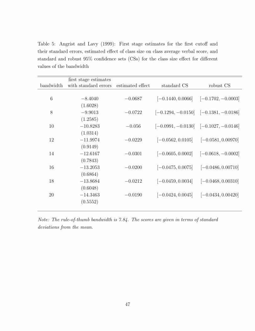
Table 5: Angrist and Lavy (1999): First stage estimates for the first cutoff andtheir standard errors, estimated effect of class size on class average verbal score, andstandard and robust 95% confidence sets (CSs) for the class size effect for differentvalues of the bandwidth

first stage estimatesbandwidth with standard errors estimated effect standard CS robust CS

6 −8.4040 −0.0687 [−0.1440, 0.0066] [−0.1702,−0.0003]

(1.6028)8 −9.9013 −0.0722 [−0.1294,−0.0150] [−0.1381,−0.0186]

(1.2585)10 −10.8283 −0.056 [−0.0991,−0.0130] [−0.1027,−0.0146]

(1.0314)12 −11.9974 −0.0229 [−0.0562, 0.0105] [−0.0581, 0.00970]

(0.9149)14 −12.6167 −0.0301 [−0.0605, 0.0002] [−0.0618,−0.0002]

(0.7843)16 −13.2053 −0.0200 [−0.0475, 0.0075] [−0.0486, 0.00710]

(0.6864)18 −13.8684 −0.0212 [−0.0459, 0.0034] [−0.0468, 0.00310]

(0.6048)20 −14.3463 −0.0190 [−0.0424, 0.0045] [−0.0434, 0.00420]

(0.5552)

Note: The rule-of-thumb bandwidth is 7.84. The scores are given in terms of standarddeviations from the mean.

47

Table 6: Angrist and Lavy (1999): Test of equality of RD effect across groups at 5%significance level for different values of the bandwidth

reject H0 of equality?bandwidth estimated effect robust standard

religious secular6 −0.0524 −0.1131 no no8 −0.0540 −0.0985 no no10 −0.0381 −0.0756 no no12 −0.0170 −0.0364 no no14 −0.0274 −0.0363 no no16 −0.0035 −0.0382 no no18 0.0052 −0.0505 yes no20 0.0107 −0.0523 yes no

<= 10% disadvantaged > 10% disadvantaged6 −0.0390 −0.0909 no no8 −0.0626 −0.0469 no no10 −0.0387 −0.0488 no no12 −0.0259 −0.0192 no no14 −0.0343 −0.0226 no no16 −0.0290 −0.0079 no no18 −0.0368 −0.0037 no no20 −0.0360 −0.0008 yes no

48

Table 7: Urquiola and Verhoogen (2009): First stage estimates for the first cutoffwith their standard errors and t-statistics for various values of the bandwidth

first-stage estimatesbandwidth with standard errors t-statistic

6 1.388 0.907(1.532)

8 −0.3873 −0.285

(1.358)10 −3.107 −2.609

(1.191)12 −4.779 −4.548

(1.051)14 −6.092 −6.406

(0.951)16 −7.87 −9.178

(0.857)18 −8.934 −11.393

(0.784)20 −9.968 −13.727

(0.726)

49

Table 8: Urquiola and Verhoogen (2009): The estimated effect of class size on theclass average math score and its 95% standard and robust confidence sets (CSs) fordifferent values of the bandwidth

bandwidth estimated effect standard CS robust CS

first cutoff (45)

6 0.146 [−0.061, 0.353] (−∞,−0.433] ∪ [0.043,∞)

8 3.378 [−74.820, 81.576] (−∞,−0.120] ∪ [0.129,∞)

10 −0.437 [−1.867, 0.993] (−∞,−0.078] ∪ [0.181,∞)

12 −0.173 [−0.360, 0.014] [−1.720,−0.065]

14 −0.136 [−0.246,−0.026] [−0.376,−0.060]

16 −0.091 [−0.153,−0.029] [−0.186,−0.042]

18 −0.073 [−0.115,−0.031] [−0.127,−0.037]

20 −0.063 [−0.099,−0.027] [−0.107,−0.032]

second cutoff (90)

6 0.128 [−0.025, 0.281] [0.004, 3.093]

8 0.261 [−0.061, 0.582] (−∞,−0.587] ∪ [0.085,∞)

10 0.227 [−0.111, 0.566] (−∞,−0.241] ∪ [0.046,∞)

12 0.306 [−0.296, 0.908] (−∞,−0.118] ∪ [0.053,∞)

14 0.486 [−1.092, 2.063] (−∞,−0.056] ∪ [0.068,∞)

16 1.636 [−18.745, 22.017] (−∞, 0.002] ∪ [0.065,∞)

18 −1.056 [−10.968, 8.856] (−∞,∞)

20 −0.425 [−2.041, 1.190] (−∞, 0.005] ∪ [0.162,∞)

The rule of thumb bandwidth is approximately 8. The scores are given in terms ofstandard deviations from the mean.

50

Table 8: (Continued)

bandwidth estimated effect standard CS robust CS

third cutoff (135)

6 −2.145 [−15.627, 11.336] (−∞,−0.076] ∪ [0.584,∞)

8 −0.298 [−0.692, 0.097] [−21.482, 0.007]

10 −0.307 [−0.850, 0.236] (−∞, 0.027] ∪ [1.414,∞)

12 −0.309 [−0.861, 0.243] (−∞, 0.027] ∪ [1.550,∞)

14 −0.328 [−0.885, 0.228] (−∞,−0.001] ∪ [1.838,∞)

16 −0.231 [−0.652, 0.190] (−∞, 0.034] ∪ [1.604,∞)

18 −0.181 [−0.500, 0.138] (−∞, 0.041] ∪ [21.933,∞)

20 −0.136 [−0.389, 0.117] [−1.642, 0.063]

forth cutoff (180)

10 0.048 [−0.119, 0.216] (−∞, ∞)

12 0.035 [−0.130, 0.200] (−∞, ∞)

14 −0.047 [−0.371, 0.278] (−∞, ∞)

16 −0.045 [−0.343, 0.254] (−∞, ∞)

18 −0.039 [−0.316, 0.238] (−∞, ∞)

20 −0.029 [−0.299, 0.242] (−∞, ∞)

51