1

Weak State Routing for Large Scale Dynamic

NetworksUtku Gunay Acer, Member, IEEE, Shivkumar Kalyanaraman, Fellow, IEEE,

and Alhussein A. Abouzeid, Member, IEEE

Abstract—Forwarding decisions in routing protocols rely oninformation about the destination nodes provided by routingtable states. When paths to a destination change, correspondingstates become invalid and need to be refreshed with controlmessages for resilient routing. In large and highly dynamicnetworks, this overhead can crowd out the capacity for datatraffic. For such networks, we propose the concept of weak state,which is interpreted as a probabilistic hint, not as absolutetruth. Weak state can remain valid without explicit messages,by systematically reducing the confidence in its accuracy. WeakState Routing (WSR) is a novel routing protocol that usesweak state along with random directional walks for forwardingpackets. When a packet reaches a node that contains a weakstate about the destination with higher confidence than that heldby the packet, the walk direction is biased. The packet reachesthe destination via a sequence of directional walks, punctuatedby biasing decisions. WSR also uses random directional walksfor disseminating routing state, and provides mechanisms foraggregating weak state.

Our simulation results show that WSR offers a very highpacket delivery ratio (≥ 98%). Control traffic overhead scalesas O(N) and the state complexity is Θ(N3/2), where N is thenumber of nodes. Packets follow longer paths compared to priorprotocols (OLSR [2], GLS-GPSR [3], [4]); but the average path

length is asymptotically efficient and scales as O(√

N). Despitelonger paths, WSR’s end-to-end packet delivery delay is muchsmaller due to the dramatic reduction in protocol overhead.

I. INTRODUCTION

In this paper, we consider the problem of designing ro-

bust and scalable routing protocols for large and dynamic

networks like large scale mobile ad-hoc networks (MANETs)

or metropolitan scale vehicular networks, where every vehicle

provides an open compute/storage/communication platform.

Though such networks are not prevalent today, they show

an immense potential for future deployment. We seek to

anticipate and understand the fundamental problem of routing,

and the nature of routing tables in such future networks.

Routing protocols in communication networks rely on rout-

ing table entries (“states”) to decide where to forward a packet.

The routing table state typically maps an ID (e.g.: destination

An earlier version of this paper appeared in MobiCom’07 [1]. The materialpresented in this paper is based upon work supported by the National ScienceFoundation under Grant No. 0546402 and 0627039. Any opinions, findings,and conclusions or recommendations expressed in this material are those ofthe authors and do not necessarily reflect the views of the National ScienceFoundation.

Utku Gunay Acer was with Rensselaer Polytechnic Institute, Troy, NY,12180, USA. He is now with INRIA Sophia Antipolis, 06902, SophiaAntipolis, France. email: utku.acer@sophia.inria.fr

Shivkumar Kalyanaraman was with Rensselaer Polytechnic Institute, Troy,NY, 12180, USA. He is now is with IBM Research - India, Bangalore, India.email: shivkumar-k@in.ibm.com

Alhussein Abouzeid is with Rensselaer Polytechnic Institute, Troy, NY,12180, USA. email: abouzeid@ecse.rpi.edu

address) or an aggregate (e.g.: a destination network) to an

entity such as a next-hop, a sequence of hops, a location

in plane etc. If a destination moves significantly within the

network, the corresponding routing table states become invalid

and need to be refreshed. As the network size increases and it

becomes more dynamic, routing table entries at several routers

must be refreshed leading to a huge increase in control traffic.

In fact, it has been recently shown that the control overhead

that is required for reliable routing may asymptotically use the

entire capacity of the network [5], [6]. On the other hand, if the

state information is not refreshed rapidly enough, the invalid

routing table entries lead to wrong routing decisions and

wandering packets that wastefully consume network capacity

without leading to end-to-end goodput.

For such large and dynamic networks, we propose to use

probabilistic routing tables, where routing table entries are

considered as probabilistic hints, and not absolute truth. Such

state information is called weak state. Weak state can be

locally refreshed by reducing the associated confidence value,

a measure of the probability that the state is accurate. This

way, weak state captures the inherent uncertainty (or weak

semantics) of the state information without the need for

explicit control traffic that traverse the network, consuming

network capacity. In other words, even though the network is

large and highly dynamic, the state information at routers is

more stable and yet useful when interpreted as probabilistic

hints. Weakening the state is similar to aging the state, albeit

in terms of semantics. The state is associated with an implicit

“soft timeout”, i.e. once the associated confidence value is

below a threshold the state is removed from the system.

We propose a novel protocol called Weak State Routing

(WSR) that uses probabilistic state information in the context

of a scalable routing protocol for large, dynamic networks.

WSR utilizes the new concept of random directional walks

(i.e. walks in randomly chosen directions) as a primitive both

for disseminating weak state, and for forwarding packets. In

particular (see Fig. 1), the source node initially assigns a

random direction to the data packet. The packet is forwarded

along this direction until it is first received by an intermediate

node that contains probabilistic information about the location

of the destination. The intermediate node biases the packet

in the direction towards this location and the new confidence

value is carried by the packet. This directional walk continues

until the packet reaches another node that contains a weak

state providing information about the destination ID with a

higher confidence value or greater accuracy of localization (i.e.

stronger state) than what is carried in the packet. The packet’s

directional walk is now biased using this information. This

2

S

D

A

B

C

E

DA

,θA D

B,θ

B

DC

,θC

DE,θ

E

Fig. 1. An illustration of routing with WSR. A data packet is forwardedfrom node S to D using random directional walks. The packet is successivelybiased in intermediate nodes, A, B, C and E in directions, towards DA, DB ,DC and DE , respectively, which the nodes believe to lead to destination. Thestrength of the bias at each intermediate node is θA, θB , θC , θE , respec-tively. Weak state biasing the packet at an intermediate node yields strongerinformation than the previously biasing state, i.e. θA < θB < θC < θE

process of the walks being biased with increasing confidence

continues until the packet reaches the destination.

The above forwarding mechanism assumes that a random

directional walk will encounter a node with probabilistic

state information about the destination with high probabil-

ity. Further, as the successively biased walk approaches the

destination, it will encounter, with high probability, nodes

with increasingly stronger state information. To support this

assumption, WSR disseminates state information periodically

in random directional walks from each node. Two random lines

(one the forwarding walk, and the other, the dissemination

walk) in a plane intersect with high probability [7]. Even with

mobility, the presence of multiple dissemination walks on the

plane that inject state at O(√

N) nodes assures that within

O(√

N) hops, with high probability, a packet forwarded in the

form of a directional walk will encounter a node that can bias

it with stronger information. WSR also provides mechanisms

for aggregating weak state to achieve scalability.

We use extensive simulations to evaluate the performance

of WSR. The simulation results show that WSR offers a

high packet delivery ratio, more than 98%. The total routing

protocol overhead scales as O(N), N being the number of

nodes. WSR offers a scalable state maintenance method by

aggregating weak states. Through asymptotical analysis, we

show that the state complexity of WSR is Θ(N3/2). The cost

of WSR is the increased path length. Even though packets fol-

low routes that are longer than the shortest paths, the average

path length is asymptotically efficient and scales as O(√

N).Despite the longer paths, due to the dramatic reduction in

control traffic overhead, the average end-to-end packet delivery

delay is much smaller than comparable protocols. In particular,

our simulations with large and dynamic networks indicate that

the average path length in WSR can be 3 times as large as

that of GLS-GPSR [3], [4] while control traffic overhead in

GLS-GPSR can be over 10 times larger than WSR overhead.

Even though the packets take longer paths with WSR, the

average end-to-end delay is up to 15 times less than that of

GLS-GPSR.

The rest of this paper is organized as follows: In Section II,

we review related work. We define our weak state concept and

present our routing mechanism in Section III. In Section IV,

we provide simulation results. We present an asymptotical

analysis in Section V. We conclude the paper in Section VI.

II. RELATED WORK

Traditional state concept can be classified into two broad

categories: hard and soft state approaches. Hard state is

maintained at a remote node until it is explicitly removed using

state-teardown messages by the node that installed the state.

Since the state is removed explicitly, reliable communication

is essential. Soft state, which was first coined in [8], times out

unless it is refreshed within a time-out duration. The node that

installed the state periodically issues refresh messages. Once

a message is received by the node maintaining the soft state,

the timer corresponding to the state is rescheduled. If the timer

expires, the state times out and it is removed from the system.

Soft state does not require explicit removal messages, unlike

hard state. Hence, reliable signaling is not required. Analytical

comparisons of hard state, soft state and the hybrid approaches

are presented in [9] and [10].In both hard state and soft state, the state information is

regarded as absolute truth. We refer to such state information

as having strong semantics or that it is an example of strong

state. When the original state changes, the strong state value

at the remote nodes should be explicitly refreshed in both

approaches (hard or soft). Weak state on the other hand has

“weak” or probabilistic semantics. The state can be refreshed

locally, by weakening or decaying the confidence value as-

sociated with the state over time. The confidence value is an

estimate of the probability that the true state is valid. Once the

confidence in the state is below a threshold value, the state is

removed from the system. Weakening the state is similar to

aging it and is equivalent to a soft timeout. Hence, weak state

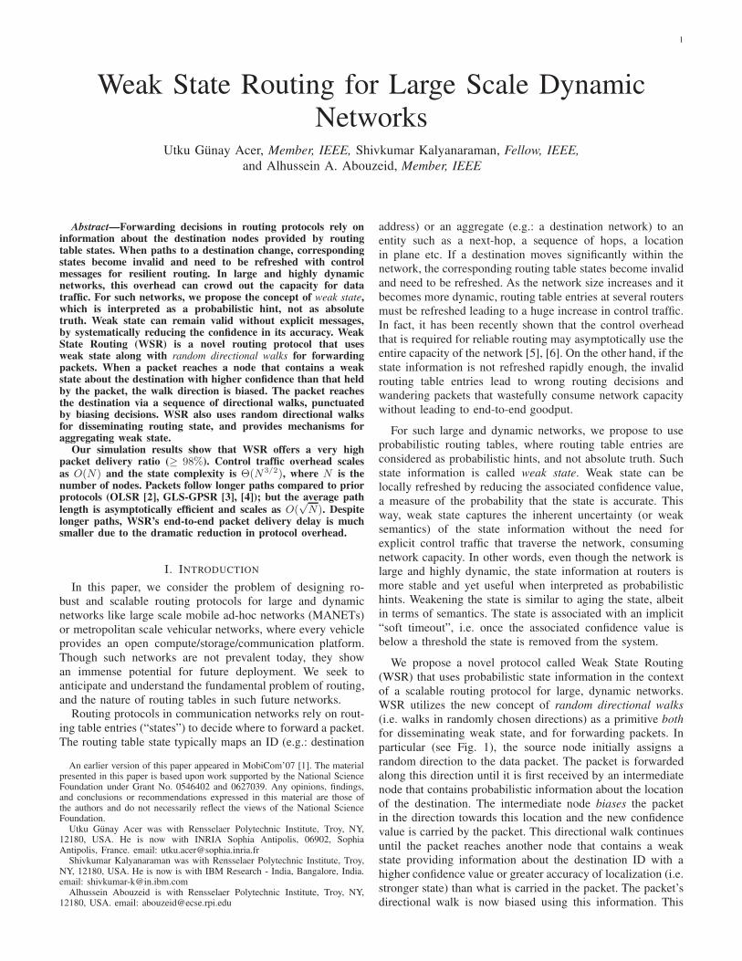
is a generalization of soft state. A comparison of hard, soft and

weak states are given in Fig. 2. The notion of state weakness

and its effect on the consistency of protocol decisions have

been evaluated in our more recent work [11], not included in

this paper.Position based routing protocols, such as Greedy Perimeter

Stateless Routing (GPSR) protocol [4], provide a scalable

solution to the routing problem (in moderately dynamic net-

works) by leveraging the geographic coordinates of nodes to

route packets. A packet is forwarded to the next-hop in the

direction of the destination. However, GPSR-like protocols

still require the knowledge of the location associated with

a destination node ID. They have to be used in conjunc-

tion with a location service protocol such as Grid Location

Service (GLS) [3] to retrieve the location information of a

destination ID. GLS partitions the network into structured

grids forming a geographical hierarchy. These structures tend

to be hard to maintain as the network size and dynamism

increase. Weak State Routing (WSR) uses the unstructured

approach of random directional walks both for forwarding

packets and disseminating state. In geographical routing, the

traditional approach isolates the location discovery (e.g. GLS)

and packet forwarding (e.g. GPSR). Even though WSR utilizes

geographical information as well, these processes take place

concurrently.

3

Sender

Receivertime

STATE A

STATE A

State removed

from the sender

State removed

from the receiver

(a) Hard State

Sender

Receivertime

STATE A

STATE A

State removed

from the sender

State refresh

interval

State timeout

intervalState removed

from the receiver

STATE A

STATE A

(b) Soft State

Sender

Receivertime

STATE A

STATE A

State removed

from the sender

State removed

from the receiver

q=1

q g<

(c) Weak State

Fig. 2. A comparison summary of hard state, soft state and weak state approaches. Hard state requires explicit control message to be removed. Soft statetimes out if it is not refreshed within the timeout interval. Weak state is associated with a confidence value θ which is a decreasing function of time. Whenthe confidence is below a threshold value γ, it is removed.

MANET routing that use link states has two subclasses:

proactive routing [12] (for large, but less dynamic networks)

and reactive or on-demand routing [13], [14] (for dynamic,

but relatively smaller networks). Recent protocols such as

FRESH [15] and EASE [16] utilize node encounter histories

as “state”. They use iterative searches to find nodes that

encountered the destination more recently. FRESH forwards a

packet to an intermediate node that encountered the destination

more recently whereas EASE sends it to the location where

the destination is encountered by such an intermediate node.

Flooding in proactive or reactive protocols to handle dy-

namism is a core issue that limits scalability. Optimized Link

State Routing (OLSR) is a link-state proactive protocol that

uses a multipoint relaying mechanism, where only a subset of

recipients redistribute control packets [2]. Hazy Sighted Link

State (HSLS) is a scalable protocol that propagates link state

information to farther nodes at decreasing rates by flooding

link state update messages with variable TTL values [17].

Though these protocols reduce flooding, they face challenges

when the network becomes both large and highly dynamic.

Increased dynamism of nodes leads to routing state updates

in a large subset of nodes, and increase in control traffic. In

addition, the cumulative number of routing table entries in

these protocols (especially OLSR) scales as O(N2). In WSR,

the cumulative state complexity is Θ(N3/2).The directional forwarding mechanism we utilize has some

similarities to the Orthogonal Rendezvous Routing Protocol

(ORRP) proposed for static networks in [7]. The paper uses

the property that a pair of orthogonal lines from the source and

destination intersect (“rendezvous”) in bounded 2-D Euclidean

space with high probability. In a mobile environment, it is

difficult to maintain fixed, orthogonal straight lines. Instead,

WSR uses random directions and requires multiple biasing

nodes to get the packet to the destination.

In Delay Tolerant Networks (DTN), some routing protocols

may maintain oracles about the global future view of the

network [18]. Opportunistic, stateless techniques are deployed

where the nodes have no global information about the network.

Instead, they rely on the natural node mobility [19], [20].

These works are inspired by Tse-Grossglauser model [21].

If the mobility scope is small relative to the size of the

network, packets may not be delivered to the destination.

PROPHET [22] positions itself between the two extremes. It

maintains transitive probabilities for each destination, such as

a probabilistic distance vector. The state information is used to

create gradients towards the destination rather than an explicit

mapping as in WSR.

Unstructured pure random walks, which proceed without

being biased, are used to locate an object in P2P networks

in [23] and [24]. In [25] and [26], Bloom filters are used

to bias random walks. Kumar et al. introduce Exponentially

Decaying Bloom Filters (EDBF) in [26], which is a “weak”

representation of a set of objects. We apply this concept to

store a probabilistic set-of-IDs. The difference between EDBF

and our weak states is that in EDBF, Bloom filters are decayed

hop-by-hop as they propagate in the network. EDBF is used to

set up implicit gradients between the nodes by comparing the

signals obtained in successive nodes. On the other hand, we

decay Bloom filters over time and use them to set up explicit

mappings from a weak set-of-IDs to a geographical region.

WSR functions as a distributed hashing method. Therefore,

WSR resembles the distributed hash tables (DHT) that provide

lookup services at large scale P2P networks [27]. In a DHT,

every node stores a range of keys and any node can locate

the node in which a particular key is stored using consistent

hashing [28]. A DHT relies on a structured overlay network.

In [29], it has been shown that maintaining such a structure

is hard and may require substantial overhead in P2P systems.

This is also true for mobile networks. A routing protocol for

wireless networks inspired by DHTs, Virtual Ring Routing

(VRR), is proposed in [30]. The authors show that increasing

the node mobility and network size degrades the network

performance significantly even though the protocol does not

require network flooding. WSR provides distributed hashing

functionality without a structured overlay as in traditional

DHTs and with more tolerance of dynamism.

GIA [29] is a scalable unstructured lookup technique for

P2P networks that depends upon the heterogeneity and lever-

ages nodes with higher storage and connectivity capabilities.

Bubblestorm [31] on the other hand hybridizes random walks

with flooding to replicate both data and queries in sub-graphs.

Once the sub-graph where the query is replicated overlaps with

the sub-graph in which requested resource is replicated, the

search is successful. With this scheme, paths are shorter than

what random walks provide and hence the delay is smaller.

Similar to GIA, Bubblestorm too exploits the heterogeneity

of nodes. In contrast, WSR can achieve similar objectives of

scaling and rare-object recall without constraints on the degree

distribution or dependence on super-nodes in the context of

large-scale dynamic networks.

III. WEAK STATE ROUTING

This section presents the details of the WSR protocol.

Specifically, we address the following:

4

�i

{1,2,3,4,a,b,c}

GeoRegion AB

GeoRegion A

2 31

4

GeoRegion B

a b

c

{1,2,3,4}

ii

{a,b,c}

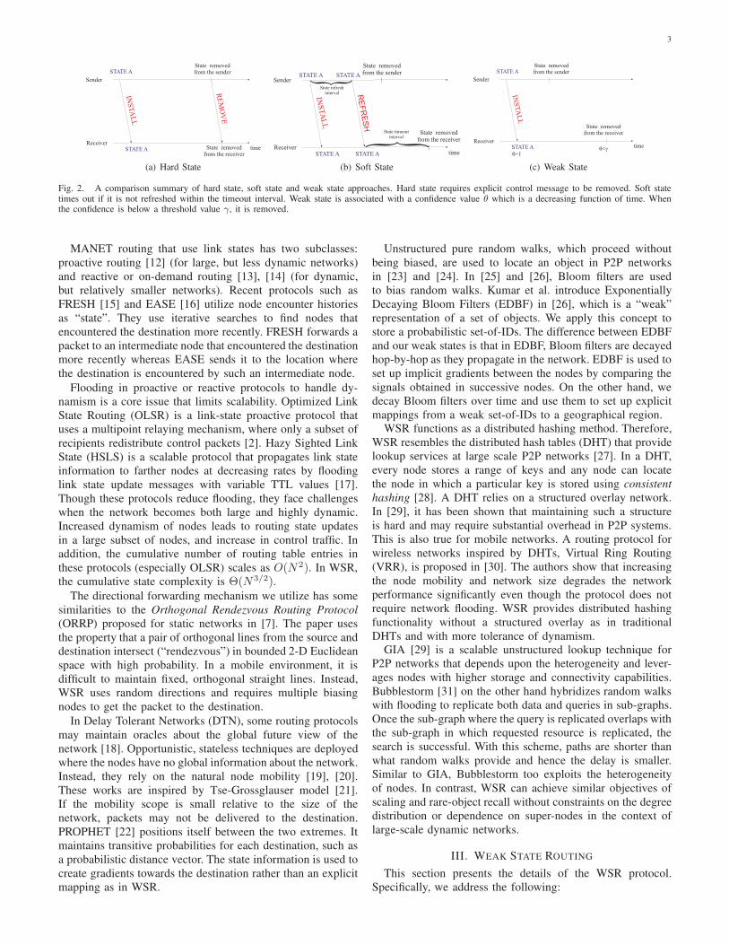
Fig. 3. Weak State Concept: A set of nodes (SetofIDs) are mapped to anaggregated geographical region (GeoRegion). Mappings are more definite forcloser nodes.

1) Assumptions made by WSR.

2) Weak state and its semantic strength

3) Proactive location announcements from destinations us-

ing random directional walks.

4) Packet forwarding strategy using successively biased

random directional walks.

A. Assumptions

The assumptions WSR makes are similar to those made by

traditional location based routing protocols: nodes know their

positions on a 2-D plane, either using a GPS device or through

any other localization techniques. By using periodic single hop

beacon messages, each node also knows its neighbors and their

positions. The nodes have uniform omni-directional antennas.

The source nodes in general do not know the location of the

destination nodes.

We consider the scenario where the nodes move indepen-

dently and the network density is high enough for connectivity

at any time. The maximum node speed is known. Though this

value can be large, we assume that the average displacement

in unit time is small in comparison to the maximum distance

between any two points in the area covered by the network.

B. Weak State Realization

In WSR, a weak state corresponds to a mapping from a

persistent node ID or a collection of IDs (SetofIDs) to a

geographical region (GeoRegion) in which the node (or the

set of nodes) is believed to be currently located. The state

information captures the uncertainty in the mapping.

An explicit mapping from a SetofIDs to a GeoRegion can be

used to “bias” the random directional walks of packets being

forwarded. If the destination ID is an element of the SetofIDs,

the packet can be biased towards the center of the associated

GeoRegion (subject to other conditions described later in this

section). The bias can be reinforced as the packets get closer

to their destinations. This is achieved by maintaining more

definite, or stronger, mappings for nodes located closer to the

destination. We capture the uncertainty in the mappings by

weakening the two components of these mappings: SetofIDs

and GeoRegion. We also aggregate the location information

about a number of nodes. In Fig. 3 for example, node i maps

node a (and a large set of nodes) to a large GeoRegion AB,

whereas node ii, which is inside this GeoRegion AB, maps a

subset of nodes to a smaller GeoRegion B. The confidence

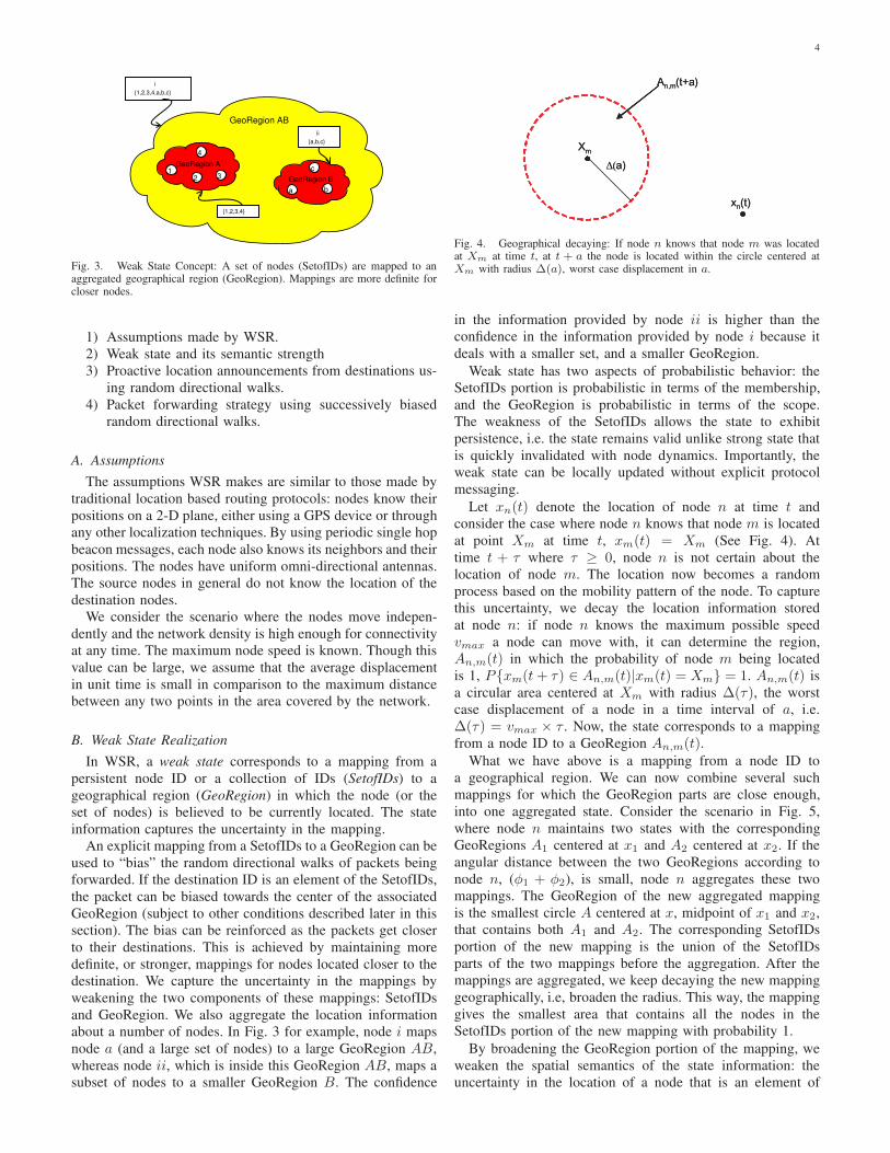
Fig. 4. Geographical decaying: If node n knows that node m was locatedat Xm at time t, at t + a the node is located within the circle centered atXm with radius ∆(a), worst case displacement in a.

in the information provided by node ii is higher than the

confidence in the information provided by node i because it

deals with a smaller set, and a smaller GeoRegion.

Weak state has two aspects of probabilistic behavior: the

SetofIDs portion is probabilistic in terms of the membership,

and the GeoRegion is probabilistic in terms of the scope.

The weakness of the SetofIDs allows the state to exhibit

persistence, i.e. the state remains valid unlike strong state that

is quickly invalidated with node dynamics. Importantly, the

weak state can be locally updated without explicit protocol

messaging.

Let xn(t) denote the location of node n at time t and

consider the case where node n knows that node m is located

at point Xm at time t, xm(t) = Xm (See Fig. 4). At

time t + τ where τ ≥ 0, node n is not certain about the

location of node m. The location now becomes a random

process based on the mobility pattern of the node. To capture

this uncertainty, we decay the location information stored

at node n: if node n knows the maximum possible speed

vmax a node can move with, it can determine the region,

An,m(t) in which the probability of node m being located

is 1, P{xm(t + τ) ∈ An,m(t)|xm(t) = Xm} = 1. An,m(t) is

a circular area centered at Xm with radius ∆(τ), the worst

case displacement of a node in a time interval of a, i.e.

∆(τ) = vmax × τ . Now, the state corresponds to a mapping

from a node ID to a GeoRegion An,m(t).What we have above is a mapping from a node ID to

a geographical region. We can now combine several such

mappings for which the GeoRegion parts are close enough,

into one aggregated state. Consider the scenario in Fig. 5,

where node n maintains two states with the corresponding

GeoRegions A1 centered at x1 and A2 centered at x2. If the

angular distance between the two GeoRegions according to

node n, (φ1 + φ2), is small, node n aggregates these two

mappings. The GeoRegion of the new aggregated mapping

is the smallest circle A centered at x, midpoint of x1 and x2,

that contains both A1 and A2. The corresponding SetofIDs

portion of the new mapping is the union of the SetofIDs

parts of the two mappings before the aggregation. After the

mappings are aggregated, we keep decaying the new mapping

geographically, i.e, broaden the radius. This way, the mapping

gives the smallest area that contains all the nodes in the

SetofIDs portion of the new mapping with probability 1.

By broadening the GeoRegion portion of the mapping, we

weaken the spatial semantics of the state information: the

uncertainty in the location of a node that is an element of

5

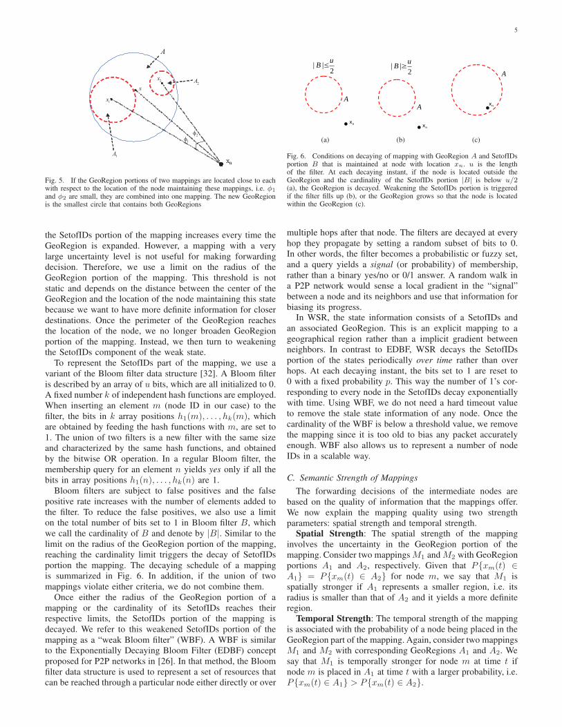
Fig. 5. If the GeoRegion portions of two mappings are located close to eachwith respect to the location of the node maintaining these mappings, i.e. φ1

and φ2 are small, they are combined into one mapping. The new GeoRegionis the smallest circle that contains both GeoRegions

the SetofIDs portion of the mapping increases every time the

GeoRegion is expanded. However, a mapping with a very

large uncertainty level is not useful for making forwarding

decision. Therefore, we use a limit on the radius of the

GeoRegion portion of the mapping. This threshold is not

static and depends on the distance between the center of the

GeoRegion and the location of the node maintaining this state

because we want to have more definite information for closer

destinations. Once the perimeter of the GeoRegion reaches

the location of the node, we no longer broaden GeoRegion

portion of the mapping. Instead, we then turn to weakening

the SetofIDs component of the weak state.

To represent the SetofIDs part of the mapping, we use a

variant of the Bloom filter data structure [32]. A Bloom filter

is described by an array of u bits, which are all initialized to 0.

A fixed number k of independent hash functions are employed.

When inserting an element m (node ID in our case) to the

filter, the bits in k array positions h1(m), . . . , hk(m), which

are obtained by feeding the hash functions with m, are set to

1. The union of two filters is a new filter with the same size

and characterized by the same hash functions, and obtained

by the bitwise OR operation. In a regular Bloom filter, the

membership query for an element n yields yes only if all the

bits in array positions h1(n), . . . , hk(n) are 1.

Bloom filters are subject to false positives and the false

positive rate increases with the number of elements added to

the filter. To reduce the false positives, we also use a limit

on the total number of bits set to 1 in Bloom filter B, which

we call the cardinality of B and denote by |B|. Similar to the

limit on the radius of the GeoRegion portion of the mapping,

reaching the cardinality limit triggers the decay of SetofIDs

portion the mapping. The decaying schedule of a mapping

is summarized in Fig. 6. In addition, if the union of two

mappings violate either criteria, we do not combine them.

Once either the radius of the GeoRegion portion of a

mapping or the cardinality of its SetofIDs reaches their

respective limits, the SetofIDs portion of the mapping is

decayed. We refer to this weakened SetofIDs portion of the

mapping as a “weak Bloom filter” (WBF). A WBF is similar

to the Exponentially Decaying Bloom Filter (EDBF) concept

proposed for P2P networks in [26]. In that method, the Bloom

filter data structure is used to represent a set of resources that

can be reached through a particular node either directly or over

(a) (b) (c)

Fig. 6. Conditions on decaying of mapping with GeoRegion A and SetofIDsportion B that is maintained at node with location xn. u is the lengthof the filter. At each decaying instant, if the node is located outside theGeoRegion and the cardinality of the SetofIDs portion |B| is below u/2(a), the GeoRegion is decayed. Weakening the SetofIDs portion is triggeredif the filter fills up (b), or the GeoRegion grows so that the node is locatedwithin the GeoRegion (c).

multiple hops after that node. The filters are decayed at every

hop they propagate by setting a random subset of bits to 0.

In other words, the filter becomes a probabilistic or fuzzy set,

and a query yields a signal (or probability) of membership,

rather than a binary yes/no or 0/1 answer. A random walk in

a P2P network would sense a local gradient in the “signal”

between a node and its neighbors and use that information for

biasing its progress.In WSR, the state information consists of a SetofIDs and

an associated GeoRegion. This is an explicit mapping to a

geographical region rather than a implicit gradient between

neighbors. In contrast to EDBF, WSR decays the SetofIDs

portion of the states periodically over time rather than over

hops. At each decaying instant, the bits set to 1 are reset to

0 with a fixed probability p. This way the number of 1’s cor-

responding to every node in the SetofIDs decay exponentially

with time. Using WBF, we do not need a hard timeout value

to remove the stale state information of any node. Once the

cardinality of the WBF is below a threshold value, we remove

the mapping since it is too old to bias any packet accurately

enough. WBF also allows us to represent a number of node

IDs in a scalable way.

C. Semantic Strength of Mappings

The forwarding decisions of the intermediate nodes are

based on the quality of information that the mappings offer.

We now explain the mapping quality using two strength

parameters: spatial strength and temporal strength.

Spatial Strength: The spatial strength of the mapping

involves the uncertainty in the GeoRegion portion of the

mapping. Consider two mappings M1 and M2 with GeoRegion

portions A1 and A2, respectively. Given that P{xm(t) ∈A1} = P{xm(t) ∈ A2} for node m, we say that M1 is

spatially stronger if A1 represents a smaller region, i.e. its

radius is smaller than that of A2 and it yields a more definite

region.

Temporal Strength: The temporal strength of the mapping

is associated with the probability of a node being placed in the

GeoRegion part of the mapping. Again, consider two mappings

M1 and M2 with corresponding GeoRegions A1 and A2. We

say that M1 is temporally stronger for node m at time t if

node m is placed in A1 at time t with a larger probability, i.e.

P{xm(t) ∈ A1} > P{xm(t) ∈ A2}.

6

Given that node m is located within a region A at time t,i.e. xm(t) ∈ A, the probability of the node being in the same

area in a future time t+τ , P{xm(t+τ) ∈ A|xm(t) ∈ A} is a

non-increasing function of τ ∈ [0,∞). Therefore, a temporal

strength parameter should capture the fact that among two

mappings, the one that provides more recent information about

a node should be temporally stronger.

In our mechanism, temporal strength of a mapping is

reduced only if the probability that a node being in that region

is not 1. In this case, we reset each 1 in the WBF part of

the mapping by a fixed collision probability, p. For a mapping

whose WBF part is denoted by B, let θ(m) = |{i; B[hi(m)] =1, i = 1, . . . , k}| be the number of 1’s in B corresponding to

node m. A larger θ(m) indicates that the mapping contains

more recent information about node m with high probability.

Therefore, the probability that the node is located within the

area that the GeoRegion portion of the mapping represents is

higher. Hence, we use θ(m) as an indicator of the temporal

strength and the value θ(m)/k as a rough (not actual) measure

of the probability P{xm ∈ A}, i.e. state confidence.

D. Dissemination of Location Information

Our routing mechanism is based on forwarding data packets

toward the region where the node believes the destination is

located, using the information given by weak states.

Initially, nodes have no information about the location of

the destination. Nodes know the location of their neighbors

through periodic beacon messages. Once two nodes which

were neighbors become non-neighbors, i.e. get out of each

other’s transmission range, they create mappings for each other

using their last known locations. For nodes farther away, WSR

uses periodic announcements from destinations in random

directions (random directional walks) to disseminate location

information. Note that a random directional walk is different

from a standard random walk; in random walks the random

walker can proceed to each neighbor with equal probability. In

random directional walks, a node selects the direction of the

announcement packet randomly and sends the announcement

in that direction, and the walk proceeds in that chosen direc-

tion. The node first picks an angle uniformly between 0 and 2πradians. The direction on which the location announcement is

sent is determined by this angle. WSR calculates the position

of a point that is far from the location of the node along this

direction (a point outside the area covered the network) and

use geographical routing to forward the announcement.

When a node receives an announcement from node m, it

creates a weak state entry: a WBF is created with bits at

indices h1(m), . . . , hk(m) are 1, and an associated GeoRegion

where the center is the location of node m and the radius is

0. After creating this state, the node checks if it can combine

this mapping with a already existing state.

By radially sending announcements in random directions

at different points in time, we increase the probability that

a packet that is also sent as random directional walk will

intersect with one of these lines on which the announcements

are sent. Also note that with this mechanism, the nodes that

are close to a particular node receive location announcements

from this node at a higher rate than the nodes further away.

Therefore, the uncertainty in the location of a node decreases

Algorithm 1 Algorithm for biasing packets in WSR

ForwardPacket (P )

1: //Consider the bias previously given to the packet P2: m← destination(P )3: θ ← Temporal(P )4: R← Spatial(P )5: (x, y)← TargetLocation(P )6: //Find the strongest local mapping indicating the where-

abouts of the node

7: for all mapping i do

8: θi ← Lookup(i, m)9: if (θi > θ) OR (θi = θ AND Ri < R) then

10: θ ← θi

11: R← Ri

12: (x, y)← Centeri

13: end if

14: end for

15: Temporal(P )← θ16: Spatial(P )← R17: TargetLocation(P )← (x, y)18: Use a geographic forwarding scheme to send the packet

to TargetLocation(P )

Lookup(i, m)

1: Φ← 02: for all q ∈ {1, 2, . . . k} do

3: Φ← Φ + WBFi[hq(m)]4: end for

5: Return Φ

as the distance to this node decreases. Even though a node has

uncertain information about the location of this destination, it

can bias the packet towards a region where the packet will

encounter a node that has more definite information.

E. Forwarding Data Packets

Our data forwarding mechanism is a simple greedy geo-

graphical forwarding algorithm, albeit using random direc-

tional walks, and consulting the weak state at intermediate

nodes. Similar to announcement packets, a data packet is ini-

tially sent in a random direction (assuming the source does not

have any weak state information about the destination). But,

unlike location announcements, a data packet is subsequently

biased at an intermediate node if the node has a weak state

about the location of the destination. We leave the problem of

acknowledgements and reliability, i.e. recovery of lost packets,

to the higher layers (transport).

The strategy we use for biasing the direction taken by data

packets at intermediate nodes is similar to the longest-prefix-

match method (summarized in Algorithm 1, called “strongest

semantics match”). We first consider the temporal strength of

the mapping to find the area that the destination node is most

likely located. To achieve this objective, the destination node

ID, m, is looked up in the WBF (i.e. SetofIDs) part of each

mapping maintained by the current node. For each mapping

i, the result of this lookup is the total number of bits set to 1

in locations indexed by hj(m), j ∈ 1 . . . k in the WBF part of

the mapping i, i.e. the temporal strength of the mapping for

7

node m, θ(m). If the temporal strength of a mapping is below

a threshold γ, the mapping is discarded. The temporal and

spatial strength values of the biasing state (i.e. the state which

influenced its current direction) are carried on the packet. If

a mapping at a subsequent node is stronger than strength

associated with the packet’s current direction (as indicated

by its header), the packet is now biased in a new direction

determined by this node’s mapping. Specifically, the node’s

state should be either temporally stronger or spatially stronger

with the same temporal strength. The packet is forwarded

toward the center of the associated GeoRegion. The actual

forwarding happens through a geographic forwarding scheme

such as GPSR. An illustration of a route determined by WSR

is given in Fig. 1. In this figure, θ values can be interpreted

as both temporal and spatial strength, with temporal strength

has priority over spatial strength.

With high probability, this mechanism does not result in

stable loops for any given packet. Specifically, we have two

cases. For Case 1, if a packet’s direction does not change,

due to the geographical forwarding, (such as GPSR), an

intermediate node does not receive a packet more than once.

For Case 2, consider the case where the packet’s direction has

changed since a node (say node-A) received the packet for

the first time. It is possible, with low probability that node-

A may receive a packet for the second time if the packet is

biased by another node (say node-B), especially if node-A

is also mobile. Since the packet has previously visited node-

A, and was subsequently biased by node-B, the most recent

bias (from node-B) is stronger than any mapping the node-

A maintains regarding the location of the destination (unless

node-A has received a new update from the destination).

Therefore (assuming node-A does not have new updates from

the destination), node-A cannot bias the packet’s direction

again. In other words, even if the packet touches a node more

than once, it does so, only in the context of making progress

towards the destination and the loop is not stable. Moreover,

since every packet is sent in an initial random direction, the

chance of multiple packets in a conversation being trapped in

loops is very small. In addition, the abrupt and sudden changes

in the node location may cause a node to receive a packet more

than once. This may lead to a persistent loop only if the node

mobility is repetitive and node speed is very high. Note that

this is not specific to WSR, but common in all geographical

routing mechanisms. Still, it is very unlikely because the node

displacement within a time interval is typically very small in

comparison to the distance traversed by a packet during the

same interval.

IV. SIMULATIONS

In this section, we evaluate the performance of WSR. We

compare WSR with OLSR and GLS location service combined

with GPSR protocol(GLS-GPSR). OLSR is an optimization of

link state protocols and does not contain flooding. Similar to

WSR, GLS is also based on a distributed hashing mechanism.

However, GLS relies on an underlying structure similar to

DHTs. In GLS-GPSR, GPSR forwarding is done after the GLS

protocol locates the geographic position of the destination.

Even though WSR uses geographical forwarding as well, loca-

tion discovery and packet forwarding take place concurrently

and cannot be isolated as in GLS-GPSR. Note that WSR itself

could be optimized further if a higher level acknowledgement

from the destination to the source conveys its location after

the first receipt of a packet (and thereby makes future packets

take shorter paths). We do not examine these optimizations in

this paper.

We empirically show that WSR achieves a high delivery

ratio, it incurs only O(N) overhead, its state complexity is

Θ(N3/2) and the average path length scales as O(√

N). We

also present how we select the WSR parameters. We obtain

the results in this section using random waypoint mobility

model [13] and with fixed node density. We also validate the

WSR performance trends with other mobility models as well.

A. Setup

In our simulations, the mobile nodes move in a square

area, which maintains an average node density of 75 nodes

per square kilometer. At the MAC layer we use IEEE 802.11

standard. The nodes have 250 m omnidirectional transmission

range.

We simulate WSR for 1000 seconds and other protocols

for 500 seconds because OLSR and GLS simulations require

too much memory. In WSR, we deploy constant bit rate

connections between 60 randomly selected source-destination

pairs. In OLSR and GLS, the number of connections is 30. For

each connection a 512 byte data packet is sent every second

for 100 seconds. All results are averaged over 5 different

instances.

The vertical bars in the graphs shown in throughout this

section correspond to the 95% confidence interval.

B. Parameter Selection

The parameters we used in our protocol are given in Table I.

We now explain the procedures for selecting WSR parameters.

In order to limit the hashing collisions in a Bloom filter to a

certain level, the number of bits in the filter, u, should increase

in the same order as the average number of nodes (IDs) a WBF

consists of. For example, if the average number of nodes in

a WBF scales as O(Nν), where ν is a constant, u should

also scale as O(Nν) in order to achieve a certain collision

probability. Therefore, the state complexity of the protocol in

terms of bits is only characterized by the average number of

nodes that an intermediate node maintains information. We

use a constant u value and a constant value for the number of

hash functions for WBFs, k. This leads to using a constant γvalue, minimum number of 1’s in a WBF that corresponds to

a node ID. If the temporal strength is below γ, the mapping is

timed out and discarded for that node ID. In our simulations,

we have u = 2048 bits, k = 32 and γ = 5.

In order to determine the decaying probability p, we look at

how long it is useful to maintain a given mapping. Remember

that the semantics of weak state is reduced over time and

the state is removed once the confidence is below a threshold

value. The time after which the state is removed is also

probabilistic. Here, we present a lower bound on the duration

for which a mapping is useful for after we start decaying

the SetofIDs portion. Note that the mapping is always useful

when we decay it geographically because the node is in the

corresponding GeoRegion with probability 1.

8

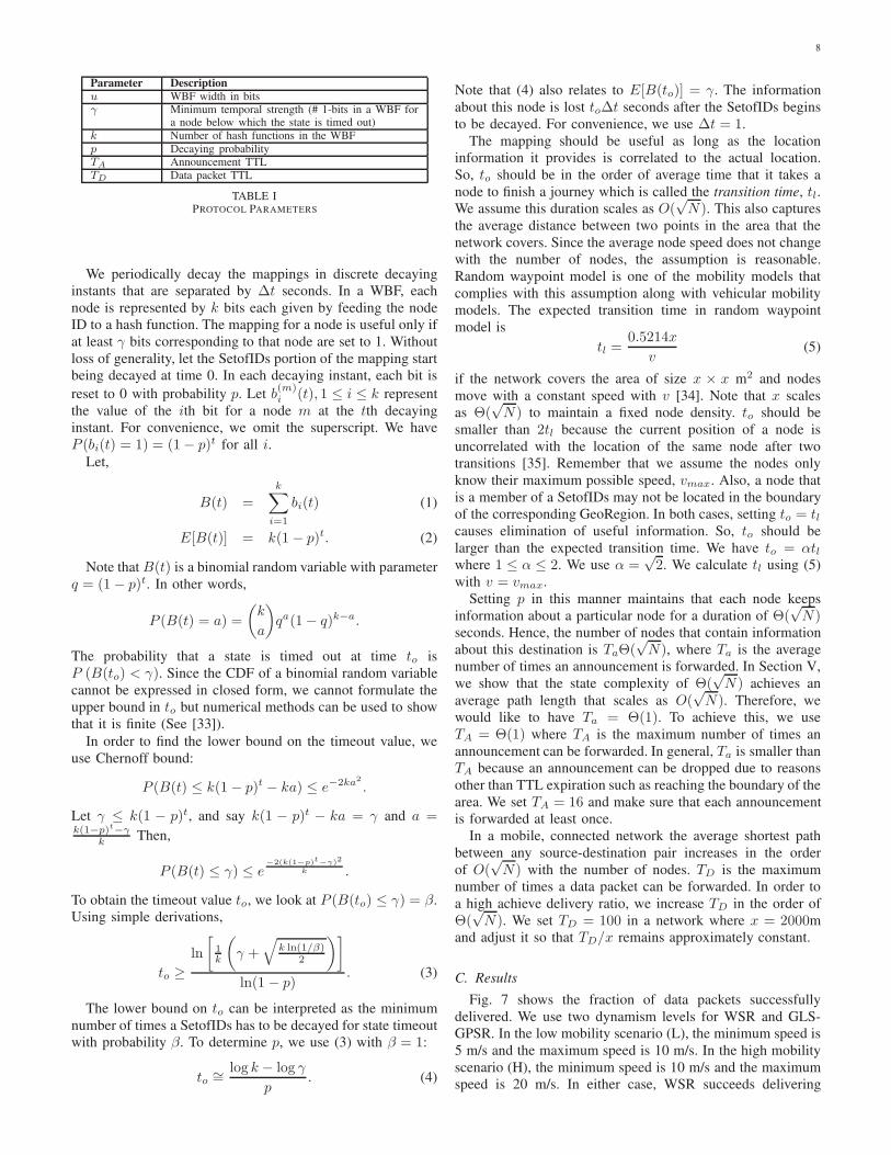
Parameter Description

u WBF width in bitsγ Minimum temporal strength (# 1-bits in a WBF for

a node below which the state is timed out)

k Number of hash functions in the WBF

p Decaying probabilityTA Announcement TTL

TD Data packet TTL

TABLE IPROTOCOL PARAMETERS

We periodically decay the mappings in discrete decaying

instants that are separated by ∆t seconds. In a WBF, each

node is represented by k bits each given by feeding the node

ID to a hash function. The mapping for a node is useful only if

at least γ bits corresponding to that node are set to 1. Without

loss of generality, let the SetofIDs portion of the mapping start

being decayed at time 0. In each decaying instant, each bit is

reset to 0 with probability p. Let b(m)i (t), 1 ≤ i ≤ k represent

the value of the ith bit for a node m at the tth decaying

instant. For convenience, we omit the superscript. We have

P (bi(t) = 1) = (1− p)t for all i.Let,

B(t) =k

∑

i=1

bi(t) (1)

E[B(t)] = k(1− p)t. (2)

Note that B(t) is a binomial random variable with parameter

q = (1− p)t. In other words,

P (B(t) = a) =

(

k

a

)

qa(1− q)k−a.

The probability that a state is timed out at time to is

P (B(to) < γ). Since the CDF of a binomial random variable

cannot be expressed in closed form, we cannot formulate the

upper bound in to but numerical methods can be used to show

that it is finite (See [33]).

In order to find the lower bound on the timeout value, we

use Chernoff bound:

P (B(t) ≤ k(1− p)t − ka) ≤ e−2ka2

.

Let γ ≤ k(1 − p)t, and say k(1 − p)t − ka = γ and a =k(1−p)t

−γk Then,

P (B(t) ≤ γ) ≤ e−2(k(1−p)t−γ)2

k .

To obtain the timeout value to, we look at P (B(to) ≤ γ) = β.

Using simple derivations,

to ≥ln

[

1k

(

γ +√

k ln(1/β)2

)]

ln(1 − p). (3)

The lower bound on to can be interpreted as the minimum

number of times a SetofIDs has to be decayed for state timeout

with probability β. To determine p, we use (3) with β = 1:

to ∼=log k − log γ

p. (4)

Note that (4) also relates to E[B(to)] = γ. The information

about this node is lost to∆t seconds after the SetofIDs begins

to be decayed. For convenience, we use ∆t = 1.

The mapping should be useful as long as the location

information it provides is correlated to the actual location.

So, to should be in the order of average time that it takes a

node to finish a journey which is called the transition time, tl.We assume this duration scales as O(

√N). This also captures

the average distance between two points in the area that the

network covers. Since the average node speed does not change

with the number of nodes, the assumption is reasonable.

Random waypoint model is one of the mobility models that

complies with this assumption along with vehicular mobility

models. The expected transition time in random waypoint

model is

tl =0.5214x

v(5)

if the network covers the area of size x × x m2 and nodes

move with a constant speed with v [34]. Note that x scales

as Θ(√

N) to maintain a fixed node density. to should be

smaller than 2tl because the current position of a node is

uncorrelated with the location of the same node after two

transitions [35]. Remember that we assume the nodes only

know their maximum possible speed, vmax. Also, a node that

is a member of a SetofIDs may not be located in the boundary

of the corresponding GeoRegion. In both cases, setting to = tlcauses elimination of useful information. So, to should be

larger than the expected transition time. We have to = αtlwhere 1 ≤ α ≤ 2. We use α =

√2. We calculate tl using (5)

with v = vmax.

Setting p in this manner maintains that each node keeps

information about a particular node for a duration of Θ(√

N)seconds. Hence, the number of nodes that contain information

about this destination is TaΘ(√

N), where Ta is the average

number of times an announcement is forwarded. In Section V,

we show that the state complexity of Θ(√

N) achieves an

average path length that scales as O(√

N). Therefore, we

would like to have Ta = Θ(1). To achieve this, we use

TA = Θ(1) where TA is the maximum number of times an

announcement can be forwarded. In general, Ta is smaller than

TA because an announcement can be dropped due to reasons

other than TTL expiration such as reaching the boundary of the

area. We set TA = 16 and make sure that each announcement

is forwarded at least once.

In a mobile, connected network the average shortest path

between any source-destination pair increases in the order

of O(√

N) with the number of nodes. TD is the maximum

number of times a data packet can be forwarded. In order to

a high achieve delivery ratio, we increase TD in the order of

Θ(√

N). We set TD = 100 in a network where x = 2000m

and adjust it so that TD/x remains approximately constant.

C. Results

Fig. 7 shows the fraction of data packets successfully

delivered. We use two dynamism levels for WSR and GLS-

GPSR. In the low mobility scenario (L), the minimum speed is

5 m/s and the maximum speed is 10 m/s. In the high mobility

scenario (H), the minimum speed is 10 m/s and the maximum

speed is 20 m/s. In either case, WSR succeeds delivering

9

400 500 600 700 800 900 10000

0.2

0.4

0.6

0.8

1

Number of Nodes

Pa

cke

t D

eviv

ery

Ra

tio

WSR (L)

GLS−GPSR (L)

OLSR (L)

WSR (H)

GLS−GPSR (H)

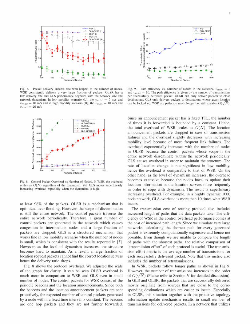
Fig. 7. Packet delivery success rate with respect to the number of nodes.WSR consistently delivers a very large fraction of packets. OLSR has alow delivery rate and GLS performance degrades with the network size andnetwork dynamism. In low mobility scenario (L), the vmin = 5 m/s andvmax = 10 m/s and in high mobility scenario (H), the vmin = 10 m/s andvmax = 20 m/s

400 500 600 700 800 900 10000

2000

4000

6000

8000

10000

12000

14000

Number of Nodes

To

tal O

ve

rhe

ad

pe

r S

eco

nd

(N

um

be

r o

f P

acke

ts)

WSR (L)

GLS−GPSR (L)

OLSR (L)

WSR (H)

GLS−GPSR (H)

Fig. 8. Control Packet Overhead vs Number of Nodes. In WSR, the overheadscales as O(N) regardless of the dynamism. Yet, GLS incurs superlinearlyincreasing overhead especially when the dynamism is high.

at least 98% of the packets. OLSR is a mechanism that is

optimized over flooding. However, the scope of dissemination

is still the entire network. The control packets traverse the

entire network periodically. Therefore, a great number of

control packets are generated in the network which causes

congestion in intermediate nodes and a large fraction of

packets are dropped. GLS is a structured mechanism that

works fine in low mobility scenario when the number of nodes

is small, which is consistent with the results reported in [3].

However, as the level of dynamism increases, the structure

becomes hard to maintain. As a result, a large fraction of

location request packets cannot find the correct location servers

hence the delivery ratio drops.

Fig. 8 shows the protocol overhead. We adjusted the scale

of the graph for clarity. It can be seen OLSR overhead is

much more in comparison to WSR and GLS even in small

number of nodes. The control packets for WSR consist of the

periodic beacons and the location announcements. Since both

the beacons and the location announcement packets are sent

proactively, the expected number of control packets generated

by a node within a fixed time interval is constant. The beacons

are one hop packets and they are not further forwarded.

400 500 600 700 800 900 10000

5

10

15

20

25

30

35

40

Number of Nodes

Tra

nsm

issio

n E

ffo

rt

(T

ran

sm

issio

ns/D

eliv

ere

d P

acke

t)

WSR

GLS−GPSR

OLSR

Fig. 9. Path efficiency vs. Number of Nodes in the Network. vmin = 5and vmax = 10. The path efficiency is given by the number of transmissionsper successfully delivered packet. OLSR can only deliver packets to closedestinations. GLS only delivers packets to destinations whose exact location

can be looked up. WSR are paths are much longer but still scalable O(√

N).

Since an announcement packet has a fixed TTL, the number

of times it is forwarded is bounded by a constant. Hence,

the total overhead of WSR scales as O(N). The location

announcement packets are dropped in case of transmission

failures and the overhead slightly decreases with increasing

mobility level because of more frequent link failures. The

overhead exponentially increases with the number of nodes

in OLSR because the control packets whose scope is the

entire network disseminate within the network periodically.

GLS causes overhead in order to maintain the structure. The

rate of location change is not significant in low mobility,

hence the overhead is comparable to that of WSR. On the

other hand, as the level of dynamism increases, the overhead

becomes excessive because the nodes have to update their

location information in the location servers more frequently

in order to cope with dynamism. The result is superlineary

increasing overhead. For example, in a highly dynamic 1000

node network, GLS overhead is more than 10 times what WSR

incurs.

The transmission cost of routing protocol also includes

increased length of paths that the data packets take. The effi-

ciency of WSR in the control overhead performance comes at

the cost of increased path length. Since we simulate very large

networks, calculating the shortest path for every generated

packet is extremely computationally expensive and hence not

possible. Even though we are unable to compare the length

of paths with the shortest paths, the relative comparison of

“transmission effort” of each protocol is useful. The transmis-

sion effort metric is the average number of transmissions for

each successfully delivered packet. Note that this metric also

includes the number of retransmissions.

In WSR, packets follow longer paths as shown in Fig 9.

However, the number of transmissions increases in the order

of O(√

N) (Please refer to Section V for detailed discussion).

In GLS and OLSR, the packets that are successfully delivered

mostly originate from sources that are close to the corre-

sponding destinations which are easier to locate. Especially

in OLSR, this situation together with the proactive topology

information update mechanism results in small number of

transmissions for delivered packets. In a network that utilizes

10

400 500 600 700 800 900 100015

20

25

30

35

40

45

Number of Nodes

Tra

nsm

issio

n E

ffo

rt

(Tra

nsm

issio

ns/D

eliv

ere

d P

acke

t)

vmin

=5, vmax

=10

vmin

=10, vmax

=10

vmin

=10, vmax

=20

Fig. 10. Path efficiency of WSR vs. Number of Nodes. The average pathlength increases with the maximum node speed but in all cases it scales as

O(√

N).

400 500 600 700 800 900 10000

0.5

1

1.5

2

2.5x 10

5

Number of Nodes

To

tal N

um

be

r o

f S

tate

s M

ain

tain

ed

WSR

GLS−GPSR

OLSR

Fig. 11. Total States Stored vs. The Number of Nodes. vmin = 5 andvmax = 10. Total storage size increases as Θ(N3/2) in WSR, O(N log N)in GLS and O(N2) in OLSR.

GLS, a node uses reactive location request packets when it has

a packet to send to a destination. For successfully delivered

packets, it is certain that the exact location of the destination

node is known. Therefore, the data packets follow the efficient

routes given by geographic forwarding scheme. We see that

average path length for delivered packets in GLS is about one

third of that in WSR.

We now look at how the path length changes with the node

mobility in WSR. In Fig. 10, we see that packets take longer

paths in the high mobility scenario. In WSR, the decaying

probability is a function of the maximum node speed. When

vmax = 20 m/s, the decaying probability is the twice the value

when vmax = 10 m/s under same conditions. As a result, the

mapping for a particular node is available for a shorter time

and it takes more transmissions for a packet to be received by

a node containing location information about the destination

for the first time.

In Fig. 11, we compare the number of mappings stored in

network in WSR with the number of entries in GLS location

database and number of entries in OLSR routing table. The

scale of the graph is adjusted for clarity. As we discuss in

Section V, the state complexity of WSR is Θ(N3/2). We

empirically see this in Fig. 11. In OLSR, every node in the

network maintains a routing table entry about every other

400 500 600 700 800 900 10000.5

1

1.5

2

2.5

3

3.5

4x 10

4

Number of Nodes

To

tal N

um

be

r o

f S

tate

s M

ain

tain

ed

vmin

=5, vmax

=10

vmin

=10, vmax

=10

vmin

=10, vmax

=20

Fig. 12. Number of mappings stored vs. Number of Nodes. Each statecorresponds to a WBF and a GeoRegion. The number of mappings stored inthe network scales as Θ(N3/2)

0 200 400 600 800 10000

5

10

15

20

25

30

35

40

45

time (seconds)

To

tal N

um

be

r o

f M

ap

pin

gs M

ain

tain

ed

pe

r N

od

e

Fig. 13. Evolution of the number of mappings in a node. The total number ofnodes in the network is 1000. vmin = 10 and vmax = 10. Announcementrate matches with the decaying aggregation rate and hence the number ofstates stored is bounded.

node in the network because the topology control packets are

received by the all the nodes in network even though OLSR

does not use flooding. Therefore, the total number of routing

table entries scales as O(N2). The total number of routing

table entries in GLS scales as O(N log N) because of the

structure it uses. This way GLS is similar to Distributed Hash

Tables and very efficient. On the other hand, WSR trades off

the number of mapping for better delivery ratio. The state

complexity is still below O(N2) and WSR can be regarded as

scalable.

Fig. 12 shows how the number of mappings stored in the

network changes with node mobility in WSR. The results

indicate that the number of mappings does not change sig-

nificantly with the increasing speed. Note that we decay the

SetofIDs portion of the mappings using a larger decaying

probability if the network is more dynamic. Still, the number

of mappings stored within the network remains roughly the

same because of aggregation. When the dynamism is low, the

average lifetime of the mappings is longer but the nodes have

more opportunities to combine mappings and vice versa in

highly dynamic scenarios. The combined effect of decaying

and aggregation mappings remains the same regardless of the

dynamism. Therefore, the number of mappings in the network

is approximately the same.

11

20 25 30 35 40 45 50 550

20

40

60

80

100

120

Number of States

Nu

mb

er

of

Occu

rre

nce

s

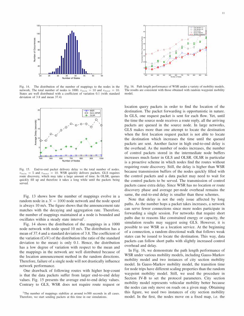
Fig. 14. The distribution of the number of mappings to the nodes in thenetwork. The total number of nodes is 1000. vmin = 10 and vmax = 10.States are well distributed with a coefficient of variation 0.1 (with standarddeviation of 3.8 and mean 37.4)

400 500 600 700 800 900 10000

5

10

15

20

25

Number of Nodes

Ave

rag

e D

ela

y (

se

co

nd

s)

WSR

GLS−GPSR

OLSR

Fig. 15. End-to-end packet delivery delay vs the total number of nodes.vmin = 5 and vmax = 10. WSR quickly delivers packets. GLS requiresroute discovery, which may take a large amount of time. In OLSR, queuesquickly fill up and therefore it takes a long while until the packets beingserved.

Fig. 13 shows how the number of mappings evolve in a

random node in a N = 1000 node network and the node speed

is always 10 m/s. The figure shows that the announcement rate

matches with the decaying and aggregation rate. Therefore,

the number of mappings maintained at a node is bounded and

oscillates within a steady state interval1.

Fig. 14 shows the distribution of the mappings in a 1000

node network with node speed 10 m/s. The distribution has a

mean of 37.4 and a standard deviation of 3.8. The coefficient of

the variation (CoV) of the distribution (the ratio of the standard

deviation to the mean) is only 0.1. Hence, the distribution

has a low degree of variation with respect to the mean and

the mappings in the network are well distributed because of

the location announcement method in the random directions.

Therefore, failure of a single node will not drastically influence

network performance.

One drawback of following routes with higher hop-count

is that the data packets suffer from larger end-to-end delay

values. Fig. 15 presents the average end-to-end delay values.

Contrary to GLS, WSR does not require route request or

1The number of mappings stabilize at around t=300 seconds in all cases.Therefore, we start sending packets at this time in our simulations.

400 450 500 550 600 650 700 750 800 850 90016

18

20

22

24

26

28

30

32

Number of Nodes

Tra

nsm

issio

n E

ffo

rt (

Tra

nsm

issio

ns/P

acke

t)

City Section (1)

City Section (2)

Community

Gauss−Markov

Random Waypoint

Fig. 16. Path length performance of WSR under a variety of mobility models.The results are consistent with those obtained with random waypoint mobilitymodel.

location query packets in order to find the location of the

destination. The packet forwarding is opportunistic in nature.

In GLS, one request packet is sent for each flow. Yet, until

the time the source node receives a route reply, all the arriving

packets are queued in the source node. In large networks,

GLS makes more than one attempt to locate the destination

when the first location request packet is not able to locate

the destination which increases the time until the queued

packets are sent. Another factor in high end-to-end delay is

the overhead. As the number of nodes increases, the number

of control packets stored in the intermediate node buffers

increases much faster in GLS and OLSR. OLSR in particular

is a proactive scheme in which nodes find the routes without

requiring route discovery. Still, the delay is higher than WSR

because transmission buffers of the nodes quickly filled with

the control packets and a data packet may need to wait for

the control packets to be served. The transmission of control

packets cause extra delay. Since WSR has no location or route

discovery phase and average per-node overhead remains the

same, the end-to-end delay is smaller than these schemes.

Note that delay is not the only issue affected by long

paths. As the number hops a packet takes increases, a network

can serve fewer connections since more nodes participate in

forwarding a single session. For networks that require short

paths due to reasons like constrained energy or capacity, the

simulation results may suggest using GLS. However, it is

possible to use WSR as a location service. At the beginning

of a connection, a random directional walk that follows weak

states can be issued to locate the destination. This way, data

packets can follow short paths with slightly increased control

overhead and delay.

In Fig. 16, we demonstrate the path length performance of

WSR under various mobility models, including Gauss-Markov

mobility model and two instances of city section mobility

model. In Gauss-Markov mobility model, the transition time

for node trips have different scaling properties than the random

waypoint mobility model. Still, we used the procedure in

Section IV-B to set the protocol parameters. City section

mobility model represents vehicular mobility better because

the nodes can only move on roads on a given map. Obtaining

this figure, we used two instances of city section mobility

model. In the first, the nodes move on a fixed map, i.e. the

12

size of the area covered by the network does not change

with the number of nodes. In the second, we used Manhattan

Grids with size that maintains a constant node density. In

all these scenarios, although the actual numbers can change,

the characteristics of WSR performance is the same: packet

delivery ratio is at least 98%, paths are longer than the shortest

paths but the average path length scales as O(√

N) and state

complexity of the protocol is O(N3/2). The difference in path

length stems from the node distribution. For example in Gauss-

Markov model, the nodes are distributed more evenly to the

area in comparison to other mobility models in which the node

distribution is denser in the center of the area. As a result,

the average path between source-destination pairs is larger in

Gauss-Markov mobility. Still, the paths are longer than the

shortest paths but the increase in the path length against the

number of nodes has the same characteristics for all mobility

models. We present the results for other performance criteria in

the extended technical report [33] because of space constraints.

V. ASYMPTOTICAL PERFORMANCE ANALYSIS

In this section, we present a simple mathematical analysis

that characterizes the asymptotical performance of our scheme.

We show that the number of mappings stored in the network

and the average path length scale as Θ(N3/2) and O(√

N),respectively. We study the notion of the weakness in terms of

consistency of protocol decisions in a separate paper [11].

A. State Complexity

The location announcements are sent along the random di-

rections with a constant TTL value. So, each announcement is

received by Θ(1) nodes. The procedure given in Section IV-B

determines the probability for decaying SetofIDs portions of

the mappings so that nodes maintain information about a

destination for a duration that scales as Θ(√

N). Within this

duration, Θ(√

N) nodes receives the location announcements

from a particular node because the announcements are sent

in random directions and the nodes move independently. This

implies that Θ(√

N) nodes maintain information about that

node and each node maintains information about Θ(√

N)nodes.

Because of the constant WBF length and the limit on the

maximum number of bits set to 1 in WBF, SetofIDs portion

of each mapping contains Θ(1) nodes. Hence, the number of

mappings a node stores scales the same way as the number of

nodes it maintains information about, i.e. Θ(√

N). Since the

WBF length is constant, this is also the number of bits a node

allocates for state storage. If we consider the entire network,

the state complexity of protocol becomes Θ(N3/2).

B. Path Length

In this section, we show that a random directional walk is

received by a node that has complete temporal strength about

the destination after it is biased by at most a constant times

and forwarded O(√

N) hops, with high probability. At this

point, the region where the destination is located is known with

certainty and we show that the probability of packet delivery

is very high within another O(√

N) hops.

Given that Θ(√

N) nodes maintain information about the

destination, the fraction of the nodes with the information

about this destination is q1 = c1√

Nwhere c1 is a constant.

Let n1 denote the number of hops a random directional walk

is forwarded until the packet first encounters a node containing

information about the destination. We have

P (n1 > n) = (1− q1)n ≤

(

1− c1√N

)n

. (6)

n1 is a geometric random variable with parameter at least q1.

Hence,

E[n1] = d1

√N (7)

where d1 is a constant. Let p1 be the probability that it is

biased at a node that has information about the destination

after it is forwarded O(√

N) times.

1− p1 =

(

1− c1√N

)b1√

N

≈ e−c1b1 . (8)

In words, a packet that is forwarded b1

√N times is biased with

an approximately high probability. This probability is high if

the product c1b1 is large.

In WSR, the protocol first checks the temporal strength of

the mappings to bias the packets. Remember that the temporal

strength of a mapping is given by the number of 1’s in the

indices that correspond to destination ID. There are a total of

k − γ temporal strength levels in the mappings (See Table I

for k and γ.). Because of the way the decaying probability is

set, the number of nodes that have a weak state with temporal

strength ω is in O(√

N) for each ω such that γ ≤ ω ≤ k.

Let θ1 denote the temporal strength of a mapping that first

biases a packet and say θ1 = ω1, where γ ≤ ω1 ≤ k.

P (θj > ω1) is the probability that a a node j has information

with a temporal strength higher than ω1. The number of nodes

that contain such information is c2

√N , with c2 < c1. The

probability that a consecutive node j, which is along the new

direction, biases the packet for the second time is denoted

by q2 and conditional on the information given by the first

mapping biasing the packet.

q2 = P (θj > ω1|θ1 = ω1).

Once the packet is biased, the direction it is forwarded is al-

tered so that it is more likely to be received by an intermediate

node that contains stronger information about the destination.

Hence, q2 is lower bounded by the unconditional probability

q2 ≥ P (θj > ω1) = c2√

N.

Based upon equations (6), (7) and (8), we can say that after

the first bias, the packet is biased again with probability p2,

which is at least a constant if it is forwarded b2

√N times.

This constant is large if c2b2 is large. The expected number

of hops the packet is forwarded between the first and second

bias, E[n2], is upper bounded by d2

√N . Because the number

of nodes that contain information with temporal strength ωis in the order of

√N for each ω, this argument is true for

every pi and ni. Note that the difference P (θj > ωi|θi =ωi)−P (θj > ωi) is larger for large values of ωi. Hence, it is

not necessarily true that E[ni] > E[ni−1] nor di > di−1.

13

The number of hops until a packet reaches a node that has

a complete temporal strength k is

ν =

K∑

i=1

ni (9)

where K is the number of times the packet is biased until it is

received by such a node. Because the number of temporal

strength values are constant (k − γ) as both k and γ are

constants, K = O(1). As a result, E[ν] = O(√

N). Similarly,

the probability that the packet is received by a node with a

mapping that has complete temporal strength k is

Pt =K∏

i=1

pi. (10)

Similar to p2, we can approximate the lower bound on each

pi as 1 − e−cibi . In the protocol, we do not control each bi.

Instead, we use a TD (See Table I) value that increases as

O(√

N), TD = b√

N as explained in Section IV-B. Using

a large b, as in our simulations, ensures that the packet is

received by a node that has a complete temporal strength about

the destination.

Once the packet is biased by a mapping with the complete

temporal strength, the region in which the destination is lo-

cated is known with certainty and the protocol makes decisions

using the spatial strength values of the mappings. The radius of

the GeoRegion part of the first mapping that biases the packet

with complete temporal strength, denoted by R1, is O(√

N).The distance between the destination and the biasing node is

also in the order of√

N hops. Once the packet is received by

a node that has a mapping with full temporal strength and a

GeoRegion with radius O(1), the packet can be delivered.

In comparison to the entire network size, the number of

nodes at which a packet can be biased via spatial strength is

small; yet, the concentration of such nodes is high in the given

GeoRegion. This is because the nodes in this region are likely

the destination’s recent neighbors and the announcements that

are sent after the one that created first mapping with complete

strength are more likely to be received by these nodes since

the announcements are sent radially.

Let us first not consider the state aggregation. Recall that we

broaden the GeoRegion portion of the mappings by periodi-

cally increasing the radius by a constant. Hence, the number of

announcements emitted by the destination since the mapping

with radius R1 hops is created is in the order of R1. If

R1 is large, the packet intersects the line on which one of

these announcement is sent (i.e. the packet is received by a

node that received that announcement) or received by a recent

neighbor of the destination with high probability. R1 is small,

the probability that the packet encounters a current neighbor

of the destination or the destination itself is high. Let this

happens after L hops. The radius of the new GeoRegion is

proportionally smaller than R1 because of the radius of the

GeoRegion is bounded.

R = O

(

1

LR1

)

(11)

Because R1 = O(√

N), after L = O(√

N) hops, the packet

reaches a node that maintains a mapping with complete

temporal strength and a GeoRegion of size O(1), that we

assume leads to final packet delivery. As a result, the total

average path length is O√

N .Recall that with state aggregation, even though the radius

of the GeoRegion increases, the deflection in the direction on

which a packet is forwarded is limited. This is because WSR

does not aggregate two mappings that are angularly far from

each other(See Fig. 5). Hence, even though the GeoRegion

of a mapping that gives fresh information about a destination

is large, forwarding the packet along the direction towards

the center of the aggregated mapping gives effectively the

same result as the forwarding the packet towards the individual

mapping.

VI. CONCLUSION AND FUTURE WORK

We present Weak State Routing (WSR) protocol, an unstruc-

tured forwarding paradigm based on the partial knowledge

about the node locations. The nodes periodically announce

their locations on random directions. The nodes use these

announcements to create aggregated SetofIDs-to-GeoRegion

mappings. A routing state consists of a weak Bloom filter

(WBF) which contains a set of nodes and a geographical

region where the nodes are believed to be located. WBF also

yields the confidence that a node is an element of SetofIDs.

When a node has a data packet, the packet is sent in a random

direction with the belief that an intermediate node will give

the packet a superior hint about the location of the destination

node. The packet trajectory is then biased toward the center

of the region indicated by this state value.In all our simulations, WSR provides a high data packet

delivery ratio greater than 98%. The total control traffic over-

head scales as O(N), where N is the number of nodes. The

state complexity of the protocol is Θ(N3/2). The average path

length is O(√

N) and asymptotically efficient in that routes

are at most a constant factor longer than the shortest path. We

show that the performance of our scheme is not affected by

the increasing mobility with speed values up to 20 m/s. Our

simulation results show that WSR significantly outperforms

OLSR and GLS with GPSR in large scale networks achieving

high reachability, low overhead and delay but needing a larger

number of hops to reach the destination.While we have considered WSR in the context of large,

mobile and connected ad-hoc networks in this paper, we

believe the weak state concept can be also adopted in networks

that experience node disconnectedness, i.e. Delay Tolerant

Networks (DTNs), though this would require different methods

for state dissemination and packet forwarding. Our future plans

include the investigation of such methods.

REFERENCES

[1] U. G. Acer, S. Kalyanaraman, and A. A. Abouzeid, “Weak State Routingfor Large Scale Dynamic Networks,” MobiCom ’07: Proceedings of the13th Annual ACM International Conference on Mobile Computing andNetworking, pp. 290–301, 2007.

[2] P. Jacquet, P. Muhlethaler, T. Clausen, A. Laouiti, A. Qayyum, andL. Viennot, “Optimized link state routing protocol for ad hoc networks,”IEEE Proceedings IEEE International Multi Topic Conference 2001.IEEE INMIC 2001. Technology for the 21st Century (Cat. No.01EX557),pp. 62 – 8, 2001.

[3] J. Li, J. Jannotti, D. De Couto, D. Karger, and R. Morris, “A scalablelocation service for geographic ad hoc routing,” Proceedings of the SixthAnnual International Conference on Mobile Computing and Network-ing(Mobicom), pp. 120 – 30, 2000.

14

[4] B. Karp and H. Kung, “GPSR: Greedy Perimeter Stateless Routing forwireless networks,” Proceedings of the Annual International Conferenceon Mobile Computing and Networking, MOBICOM, pp. 243 – 254, 2000.

[5] N. Bisnik and A. A. Abouzeid, “Capacity Deficit in Mobile Wireless AdHoc Networks Due to Geographic Routing Overheads,” in 26th IEEE In-ternational Conference on Computer Communications (INFOCOM’07).,2007, pp. 517–525.

[6] D. Wang and A. A. Abouzeid, “Link state routing overhead in mobilead hoc networks: A rate-distortion formulation,” Proceedings - IEEEINFOCOM, pp. 2011 – 2019, 2008.

[7] B.-N. Cheng, M. Yuksel, and S. Kalyanaraman, “Orthogonal rendezvousrouting protocol for wireless mesh networks,” IEEE/ACM Transactionson Networking, vol. 17, no. 2, pp. 542 – 555, 2009.

[8] D. D. Clark, “The design philosophy of the DARPA internet protocols,”in SIGCOMM. ACM, 1988, pp. 106–114.

[9] S. Raman and S. McCanne, “Model, analysis, and protocol frameworkfor soft state-based communication,” Computer Communication Review,vol. 29, no. 4, pp. 15 – 25, 1999.

[10] P. Ji, Z. Ge, J. Kurose, and D. Towsley, “A comparison of hard-state andsoft-state signaling protocols,” IEEE/ACM Transactions on Networking,vol. 15, no. 2, pp. 281 – 294, 2007.

[11] U. G. Acer, A. Abouzeid, and S. Kalyanaraman, “An Evaluation ofWeak State Mechanism Design for Indirection in Dynamic Networks,”INFOCOM’09: The 28th IEEE International Conference on ComputerCommunications, pp. 1125–1133, 2009.

[12] C. E. Perkins and P. Bhagwat, “Highly dynamic destination-sequenceddistance-vector routing (DSDV) for mobile computers,” Computer Com-munications Review, vol. 24, no. 4, pp. 234 –, 1994.

[13] D. B. Johnson and D. A. Maltz, “Dynamic Source Routing in Ad HocWireless Networks,” in Mobile Computing, T. Imielinski and H. Korth,Eds. Kluwer Academic Publishers, 1996, vol. 353.

[14] C. E. Perkins and E. Royer, “Ad-hoc on-demand distance vector routing,”Second IEEE Workshop on Mobile Computing Systems and Applications.WMCSA ’99., pp. 90–100, 1999.

[15] H. Dubois-Ferriere, M. Grossglauser, and M. Vetterli, “Age matters:Efficient route discovery in mobile ad hoc networks using encounterages,” Proceedings of the International Symposium on Mobile Ad HocNetworking and Computing (MobiHoc), pp. 257 – 266, 2003.

[16] M. Grossglauser and M. Vetterli, “Locating mobile nodes with EASE:Learning efficient routes from encounter histories alone,” IEEE/ACMTransactions on Networking, vol. 14, no. 3, pp. 457 – 469, 2006.

[17] C. Santivanez and R. Ramanathan, “Hazy Sighted Link State (HSLS)Routing: A Scalable Link state Algorithm,” BBN Technologies, Cam-bridge, MA, Tech. Rep. BBN-TM-1301, 2001.

[18] S. Jain, K. Fall, and R. Patra, “Routing in a delay tolerant network,”Computer Communication Review, vol. 34, no. 4, pp. 145 – 157, 2004.

[19] T. Spyropoulos, K. Psounis, and C. S. Raghavendra, “Spray and wait:An efficient routing scheme for intermittently connected mobile net-works,” Proceedings of ACM SIGCOMM 2005 Workshops: Conferenceon Computer Communications, pp. 252 – 259, 2005.

[20] Y. Wang, S. Jain, M. Martonosi, and K. Fall, “Erasure-coding basedrouting for opportunistic networks,” Proceedings of ACM SIGCOMM2005 Workshops: Conference on Computer Communications, pp. 229 –236, 2005.

[21] M. Grossglauser and D. N. Tse, “Mobility increases the capacity of adhoc wireless networks,” IEEE/ACM Transactions on Networking, vol. 10,no. 4, pp. 477 – 486, 2002.

[22] A. Lindgren, A. Doria, and O. Schelen, “Probabilistic routing in in-termittently connected networks,” Service Assurance with Partial andIntermittent Resources. First International Workshop, SAPIR 2004. Pro-ceedings (Lecture Notes in Comput. Sci. Vol.3126), pp. 239 – 54, 2004.

[23] Q. Lv, P. Cao, E. Cohen, K. Li, and S. Shenker, “Search and replicationin unstructured peer-to-peer networks,” Proceedings of the InternationalConference on Supercomputing, pp. 84 – 95, 2002.

[24] C. Gkantsidis, M. Mihail, and A. Saberi, “Random walks in peer-to-peernetworks,” Proceedings - IEEE INFOCOM, vol. 1, pp. 120 – 130, 2004.

[25] S. C. Rhea and J. Kubiatowicz, “Probabilistic location and routing,”Proceedings - IEEE INFOCOM, vol. 3, pp. 1248 – 1257, 2002.

[26] A. Kumar, J. Xu, and E. W. Zegura, “Efficient and scalable queryrouting for unstructured peer-to-peer networks,” Proceedings of IEEEINFOCOM, vol. 2, pp. 1162 – 1173, 2005.

[27] I. Stoica, R. Morris, D. Liben-Nowell, D. R. Karger, M. F. Kaashoek,F. Dabek, and H. Balakrishnan, “Chord: a scalable peer-to-peer lookupprotocol for internet applications,” IEEE/ACM Transactions on Network-ing, vol. 11, no. 1, pp. 17–32, 2003.

[28] D. Karger, E. Lehman, T. Leighton, M. Levine, D. Lewin, and R. Pan-igrahy, “Consistent hashing and random trees: Distributed cachingprotocols for relieving hot spots on the world wide web,” Conference

Proceedings of the Annual ACM Symposium on Theory of Computing,pp. 654 – 663, 1997.

[29] Y. Chawathe, S. Ratnasamy, L. Breslau, N. Lanham, and S. Shenker,“Making Gnutella-like P2P Systems Scalable,” Computer Communica-tion Review, vol. 33, no. 4, pp. 407 – 418, 2003.

[30] M. Caesar, M. Castro, E. B. Nightingale, G. O’Shea, and A. Rowstron,“Virtual ring routing: Network routing inspired by DHTs,” ComputerCommunication Review, vol. 36, no. 4, pp. 351 – 362, 2006.

[31] W. W. Terpstra, J. Kangasharju, C. Leng, and A. P. Buchmann, “Bub-bleStorm: resilient, probabilistic, and exhaustive Peer-to-Peer search,” inProceedings of the 2007 ACM SIGCOMM Conference. New York, NY,USA: ACM Press, Aug. 2007, pp. 49–60.

[32] B. H. Bloom, “Space/Time Trade-offs in Hash Coding with AllowableErrors,” Communications of the ACM, vol. 13, no. 7, pp. 422–426, 1970.

[33] U. G. Acer, S. Kalyanaraman, and A. A. Abouzeid, “Weak State Routingfor Large Scale Dynamic Networks (Extended Paper),” http://networks.ecse.rpi.edu/∼acer/wsr extended.pdf, Electrical, Computer and SystemsEngineering Department, Rensselaer Polytechnic Institute, Tech. Rep.,2009.

[34] C. Bettstetter, H. Hartenstein, and X. Perez-Costa, “Stochastic propertiesof the random waypoint mobility model,” Wireless Networks, vol. 10,no. 5, pp. 555 – 567, 2004.

[35] E. Hyytia, P. Lassila, and J. Virtamo, “Spatial node distribution of therandom waypoint mobility model with applications,” IEEE Transactionson Mobile Computing, vol. 5, no. 6, pp. 680 – 693, 2006.

Utku Gunay Acer received his B.S. degree intelecommunications engineering with honors fromSabancı University, Turkey in 2004 and his PhDdegree from the Electrical, Computer and SystemsEngineering Department of Rensselaer PolytechnicInstitute in 2009. Since October 2009, he has beena post-doctoral researcher with the National Re-search Institute of Informatics and Control (INRIA),Sophia-Antipolis, France. His current research in-terests include performance evaluation and protocoldesign for variable topology networks and with an

emphasis on large scale ad-hoc and disruption tolerant networks. He is amember of IEEE.

Shivkumar Kalyanaraman is with IBM Research- India, Bangalore. Previously he was a Professor atthe Department of Electrical, Computer and SystemsEngineering at Rensselaer Polytechnic Institute inTroy, NY. He holds a Computer Science B.Techdegree from IIT, Madras, India, and M.S., Ph.D.degrees from Ohio State University. His researchinterests include various traffic management topicsand protocols for emerging tetherless networks. Heis a senior member of the ACM and a Fellow ofIEEE.

Alhussein A. Abouzeid received the B.S. degreewith honors from Cairo University, Cairo, Egyptin 1993, and the M.S. and Ph.D. degrees fromUniversity of Washington, Seattle, WA in 1999 and2001, respectively, all in electrical engineering.

He is currently Associate Professor of Electri-cal, Computer, and Systems Engineering, and co-founding Deputy Director of the Center for Perva-sive Computing and Networking, Rensselaer Poly-technic Institute (RPI), Troy, NY. Since December2009, he has been on leave from RPI, serving as

Program Director, Computer & Network Systems Division, Computer &Information Science & Engineering Directorate, National Science Foundation,Arlington, VA. From 1994 to 1997, he was a Project Manager in Alcateltelecom. From 1993 to 1994 he was with the Information Technology Institute,Information and Decision Support Center, The Cabinet of Egypt. He receivedthe Faculty Early Career Development Award (CAREER) from the USNational Science Foundation in 2006. He is a member of IEEE and ACMand serves on the technical program and executive committees of variousconferences. He is also a member of the editorial board of Computer Networks(Elsevier).