econstorMake Your Publication Visible

A Service of

zbwLeibniz-InformationszentrumWirtschaftLeibniz Information Centrefor Economics

Cheung, Yin-Wong; Steinkamp, Sven; Westermann, Frank

Working Paper

China's Capital Flight: Pre- and Post-CrisisExperiences

CESifo Working Paper, No. 5584

Provided in Cooperation with:Ifo Institute – Leibniz Institute for Economic Research at the University ofMunich

Suggested Citation: Cheung, Yin-Wong; Steinkamp, Sven; Westermann, Frank (2015) : China'sCapital Flight: Pre- and Post-Crisis Experiences, CESifo Working Paper, No. 5584

This Version is available at:http://hdl.handle.net/10419/123220

Standard-Nutzungsbedingungen:

Die Dokumente auf EconStor dürfen zu eigenen wissenschaftlichenZwecken und zum Privatgebrauch gespeichert und kopiert werden.

Sie dürfen die Dokumente nicht für öffentliche oder kommerzielleZwecke vervielfältigen, öffentlich ausstellen, öffentlich zugänglichmachen, vertreiben oder anderweitig nutzen.

Sofern die Verfasser die Dokumente unter Open-Content-Lizenzen(insbesondere CC-Lizenzen) zur Verfügung gestellt haben sollten,gelten abweichend von diesen Nutzungsbedingungen die in der dortgenannten Lizenz gewährten Nutzungsrechte.

Terms of use:

Documents in EconStor may be saved and copied for yourpersonal and scholarly purposes.

You are not to copy documents for public or commercialpurposes, to exhibit the documents publicly, to make thempublicly available on the internet, or to distribute or otherwiseuse the documents in public.

If the documents have been made available under an OpenContent Licence (especially Creative Commons Licences), youmay exercise further usage rights as specified in the indicatedlicence.

www.econstor.eu

China’s Capital Flight: Pre- and Post-Crisis Experiences

Yin-Wong Cheung Sven Steinkamp

Frank Westermann

CESIFO WORKING PAPER NO. 5584 CATEGORY 7: MONETARY POLICY AND INTERNATIONAL FINANCE

OCTOBER 2015

An electronic version of the paper may be downloaded • from the SSRN website: www.SSRN.com • from the RePEc website: www.RePEc.org

• from the CESifo website: Twww.CESifo-group.org/wp T

ISSN 2364-1428

CESifo Working Paper No. 5584

China’s Capital Flight: Pre- and Post-Crisis Experiences

Abstract We study China’s illicit capital flow and document a change in its pattern. Specifically, we observe that China’s capital flight, especially the one measured by trade misinvoicing, exhibits a weakened response in the post-2007 period to the covered interest disparity, which is a theoretical determinant of capital flight. Further analyses indicate that the post-2007 behavior is influenced by quantitative easing and other factors including exchange rate variability, capital control policy and trade frictions. Our study confirms that China’s capital flight pattern and its determinants are affected by the crisis event. Further, both the canonical and additional explanatory variables have different effects on different measures of capital flight. These results highlight the challenges of managing China’s capital flight, which requires information on the period and the type of capital flight that the policy authorities would like to target.

JEL-Codes: F300, F320, G150.

Keywords: world bank residual method, trade misinvoicing, quantitative easing, capital controls, covered interest disparity.

Yin-Wong Cheung Hung Hing Ying Chair

City University Hong Kong Kowloon / Tong / Hong Kong

yicheung@cityu.edu.hk

Sven Steinkamp Institute of Empirical Economic Research

Osnabrück University Germany – 49069 Osnabrück

sven.steinkamp@uni-osnabrueck.de

Frank Westerman* Institute of Empirical Economic Research

Osnabrück University Germany – 49069 Osnabrück

frank.westermann@uni-osnabrueck.de

*corresponding author

1

1. Introduction

China is increasingly integrated with the global economy. The pace of integration, however,

is uneven across the trade and financial sectors. Since its reform initiatives were launched in 1978,

China has gradually evolved from a closed and isolated economy to the world’s largest trading

nation. While liberalizing trade activity, China is quite conscientious about the stability of its

financial sector. Regulations and capital control measures are in place to restrict and manage

cross-border capital movements. Despite the fact that China is loosening its grip on its financial

markets, it maintains explicit controls on capital account transactions to manage its

underdeveloped financial sector and protect it from external financial volatility.1

China’s capital control measures target both inflows and outflows. While excessive capital

inflows overheat the domestic economy, massive outflows drain needed resources from

development projects and impose pressure on monetary and exchange rate policies. One

commonly discussed caveat of China’s capital account liberalization policy is the capital outflow

and its adverse economic impacts that may occur when China opens up its capital account

(Bayoumi and Ohnsorge, 2013). Despite China’s infamously tight grip on its capital account, it

cannot perfectly regulate money movement across its border.

In the last few decades, China has been adjusting its capital control policy to maintain a

stable economic environment for its reform initiatives. Hung (2008) and Prasad and Wei (2007),

for instance, describe China’s policy measures aimed at curbing illicit capital flows. Although

these capital control measures are deemed effective, they do not eliminate all illicit flows.

Cheung and Herrala (2014), and Ma and McCauley (2008) for example, show that China’s

control of cross-border capital movement is porous. While control measures deter money from

moving across borders, people find ways to circumvent these barriers. The magnitude of China’s

capital flight could be quite large. For some years, inward or outward capital flight could be

larger than the official foreign direct investment data or the change in external debts (Cheung and

Qian, 2010).

Anecdotal evidence indicates that sizable capital flight – both inward and outward – has

taken place in China. It is commonly believed that China’s outward capital flight is driven by the

desire to move money out of a tightly controlled regime. For different reasons, wealthy

1 Fernald and Babson (1999) and Yu (2009), for instance, attribute to capital controls China’s ability to insulate

itself from the massive external financial volatility in the recent global financial crises.

2

individuals and corrupted executives/officials choose to shelter their wealth overseas. The

anticorruption campaign launched by the Xi Jinping regime reveals and reaffirms the widespread

existence of corruption and the magnitude of capital flight related to the embezzlement of public

funds. Inward capital flight sometimes is perceived to be hot money that takes advantage of the

flourishing real estate sector, shadow banking, and equity market.

Financial crises in the last few decades have always reminded authorities of the detrimental

impact of volatile cross-border capital flows on their economies. The 2007/8 Global Financial

Crisis is no exception. One new phenomenon of the recent crisis and its aftermath is

characterized by an ultra-loose monetary policy, dubbed quantitative easing pursued by the

United States to revive its economy. A similar accommodative monetary policy has been

subsequently pursued by other economies including Great Britain, Japan and the European

Monetary Union. The developing and emerging economies including China in general are quite

concerned about the massive capital inflows triggered by excess global liquidity created by

quantitative easing. Typically, these economies have tightened their policies on cross-border

capital movements to alleviate destabilizing capital flows. Indeed, China was quite vigilant – it

strengthened its management of capital flows in general, and, in June 2008, explicitly reinstated

its managed exchange rate policy in particular.

In this article, we empirically analyze China’s capital flight. The choice of China is

motivated by its growing importance on the global stage and the relative size of its capital flight.

Kar and Spanjers (2014) for instance, assert that China is the leading source of illicit capital flows

among developing countries, and it dominates the flows originating from Asia.2

Our exercise considers two approaches to generate a proxy for capital flight. The first, the

commonly used World Bank residual approach, uses balance-of-payments statistics and generates

the proxy from the difference between the sources and uses of funds (Cuddington, 1987, 1986;

World Bank, 1985).

The second approach is based on the notion of trade misinvoicing, which is believed to be a

common business maneuver to bypass controls and move money across national borders. For

instance, export underinvoicing and import overinvoicing facilitate outward capital flight. Kar

and Freitas (2012) and Kar and Spanjers (2014) estimate trade misinvoicing to account for 77.8%

2 Laws and rules restricting foreign purchases of assets instituted in the 2000s by, for example, Singapore and

Australia were perceived to target capital inflows from China. The top five sources of outward capital flight from 2003 to 2012 are China, Russia, Mexico, India, and Malaysia.

3

of total capital flight. This is a significant source of China’s capital flight, too. The asserted role

of trade misinvoicing echoes China’s repeated efforts to curtail trade misinvoicing by cracking

down on forged, illegal, and reused trade documents.

Using these measures, we compare the patterns of China’s capital flight before and after the

2007/8 global financial crisis in light of its dramatic impacts on the global market and related

policy responses. In anticipation of the empirical results, we show that the World Bank residual

and the trade misinvoicing measures of China’s capital flight behave differently, and these

measures exhibit different patterns before and after the eruption of the crisis. Further, the change

in behavior could be related to the ultra-accommodative monetary policy adopted by, for example,

the United States after the crisis, and to the responses to exchange rate variability and control

policy measures.

The next section introduces the World Bank residual and trade misinvoicing measures of

capital flight, presents the basic capital flight regression specifications, and lists the explanatory

variables that comprise both canonical economic determinants and factors specific to China.

Section 3 extends the basic specifications to accommodate different behaviors in the post-crisis

period and explores several potential factors driving the behavior in the post-crisis period. Some

robustness regressions are presented in Section 4. Section 5 concludes.

2. Basics

2.1 Two Capital Flight Measures

There is little disagreement on the adverse effect of capital flight, which hinders the capital-

formation and resource-allocation processes and strains the financial system.3 Its exact definition,

however, is far from conclusive. One general interpretation equates capital flight to capital

movement triggered by economic and political uncertainty. An obvious drawback of this

interpretation is that accurately measuring it is difficult.4 In the current study, we consider two

operationally feasible notions of capital flight that are commonly used in the literature. They are

the World Bank residual measure and the trade misinvoicing measure.

The World Bank residual measure of capital flight is quite routinely adopted in empirical

studies. Using information from balance-of-payments statistics to determine the discrepancy of

3 Capital flight could be beneficial if it helps circumvent distortionary capital controls and trade barriers. 4 Discussions of various measures of capital flight and their limitations are given in, for example, Claessens and

Naude (1993), Kant (1996), Kar and Cartwright-Smith (2009), Schneider (2003), and Zhao et al. (2013).

4

the uses and sources of funds, the measure provides an operational definition of capital flight.

There is outward (inward) capital flight when the total source of funds is larger (less) than the

total use of funds. Building on publicly available national accounting information, the World

Bank residual measure covers a wide range of economic activities including all foreign assets and

liabilities incurred by both public and private sectors. This measure is also replicated easily.

The World Bank residual method (World Bank, 1985) computes capital flight according to

WBR = ∆ExD + NFDI – CAD – ∆IR, (1)

where the sources of funds are given by the change in external debts (∆ExD) and the net foreign

direct investment (NFDI), and the uses of funds are the current account deficit (CAD) and the

change in international reserves (∆IR). If all international transactions are properly reported, the

double-entry accounting practice will ensure that the uses of funds equal the sources of funds and

the World Bank residual (WBR) measure is zero.

When the sources of funds are larger than the uses, the difference is interpreted as

unreported illicit capital outflow. When capital is leaking from the economy, it reflects dislike of

domestic assets and resources are leaving. When the sources of funds are less than the uses,

foreign capital is infiltrating into the domestic economy, and there is a relative preference for

domestic assets. The current study uses data from China’s State Administration of Foreign

Exchange to construct the WBR measure.

Trade misinvoicing is a well-documented way to circumvent regulations and move money

illicitly across national borders (Bhagwati, 1981, 1964; Cardoso and Dornbusch, 1989). To

quantify the level of trade misinvoicing, we compare the trade data reported by China and its

trading partners. The trade data are from the Directions of Trade Statistics. One practical

technical issue is that export data are reported at f.o.b. (free on board) prices and imports are at

c.i.f. (cost, insurance and freight) prices. Even in the absence of misinvoicing behavior, the two

price conventions create a wedge between trade data reported by importing and exporting

countries. To allow for differences in reported prices, we incorporate a variable CIF to capture

the c.i.f. effect in calculating China’s export underinvoicing, EUI,

EUI = [XWi,t – XCi,t*(1+CIF)], (2)

where XWi,t is economy i’s reported value of imports from China, XCi,t is China’s reported value

of exports to country i, p is the number of economies importing from China, and CIF facilitates a

pi

5

fair comparison of the reported values of exports and imports. In the current and next sections,

CIF assumes the value of 10%, a value commonly adopted by recent studies on trade

misinvoicing. 5 The results based on alternative fixed and time-varying values of CIF are

discussed in Section 4. A positive EUI implies China underinvoiced or underreported the value of

its exports, and capital has been illicitly transferred to its trading partners.6 By the same token, we

calculate China’s import overinvoicing, IOI as

IOI = [MCi,t – MWi,t*(1+CIF)]. (3)

MCi,t is China’s reported value of imports from country i, MWi,t is economy i’s reported

value of exports to China, and q is the number of countries exported to China. Again, a positive

IOI implies capital is leaking out of China.

The amount of China’s capital flight via trade misinvoicing is the sum of export

underinvoicing and import overinvoicing; that is, TMI = EUI + IOI. Henceforth, the sum is called

the trade misinvoicing (TMI) measure of capital flight.

The WBR and the TMI measures normalized by the gross domestic product (GDP) are

plotted in Figure 1. The sample period ranges from 1998:Q1 to 2014:Q2. Apparently, the two

measures evolve differently during the sample period, with a statistically insignificant sample

correlation of −0.0398.

The TMI measure indicates money was moving out of China for most of the sample period

until the post-crisis period. Starting roughly after 2009, the measure suggests that capital was

moving into China via TMI. The WBR measure, to a lesser extent, also exhibits a different

behavior after the 2007/8 global financial crisis. In contrast to the TMI measure, the WBR

measure shows a strong (average) outward capital flight in the post-crisis period.

The weak correlation suggests the possibility that the two measures capture different

aspects of China’s capital flight phenomenon. The WBR measure is based on international

transactions reported by China in its balance-of-payments statistics. The TMI measure focuses on

misreporting of trade transactions. Data from China and its trade partners are used to infer the

extent of misreporting. TMI could be carried out via price and quality misrepresentation, and

faked, forged, or illegally reused trade documents. Both discrepancies in coverage and data

5 See, for example, Beja (2008) and Kar and Freitas (2012). The value of 10% corresponds to the IMFs estimate

(International Monetary Fund, 2015, 2010, 1993). 6 We implicitly assume that EUI is mainly driven by China’s invoicing behavior.

qi

6

source contribute to differences of these two measures. Further, these two types of illicit cross-

border capital transfers are likely to be committed by different segments of the population.

The official capital flow based on financial account information is included in Figure 1. For

comparison purposes, the official data adopt the sign convention of the capital flight measure;

that is, a positive (negative) number means outflow (inflow). During the sample period, there are

on average substantial official capital inflows – an observation in line with China’s large trade

surplus and strong FDI performance. The sizes of the two capital flight measures, however, are at

times comparable to that of the official flow; a phenomenon also noted in Cheung and Qian

(2010).7,8 Thus, China’s capital flight seems to be non-negligible relative to the official flow.

Given that the WBR measure and the TMI measure have a weak correlation and can capture

different facets of China’s capital flight, we include the sum of the two measures as a third

measure of capital flight in the subsequent analysis.9 For brevity, we label the sum as the

combined measure (CM) of capital flight. The combined measure is plotted in Figure 1c. The

correlation of the combined measure with its two components are, respectively 0.7613 (WBR

measure) and 0.6176 (TMI measure).

FIGURE 1 HERE

2.2 Preliminary Results

A bivariate empirical specification of capital flight derived from the portfolio balance

approach (Cuddington, 1986; Diwan, 1989; Dornbusch, 1984) is given by

Yt = α + λCIDt + εt, (4)

where Yt is the capital flight normalized by GDP, CIDt is the deviation from the covered interest

parity between the Chinese and US currencies.10 Money tends to flow out from an economy when

its return on capital after adjusting for currency gains/losses is lower than in the rest of the world.

7 The averages of the net official flows, the WBR measure, and the TMI measure are, respectively, −0.61, 0.12, and

0.72 during the sample period. 8 The official flow and the WBR measure in fact have a quite high level of association, with an estimated sample

correlation coefficient of 0.74. However, the official flow data have essentially zero correlation with the TMI measure; their sample correlation coefficient estimate is almost zero and insignificant.

9 The combined estimate is considered in, for example, Boyce and Ndikumana (2001), Collier et al. (2001), Gunter (2004, 1996), and Kar and Spanjers (2014).

10 In the empirical literature, both capital flight and cumulative capital flight are examined. For instance, Boyce (1992), Cerra et al. (2008), Fedderke and Liu (2002); Le and Zak (2006); Lensink et al. (2000); Mikkelsen (1991), Ndikumana and Boyce (2003) and Pastor (1990) examined capital flight, while Cheung and Qian (2010), Collier et al. (2001), Cuddington (1987), Dooley (1988) and Rojas-Suarez (1990) considered cumulative capital flight. We consider the former, as it is the usual object of the policy debate.

7

Covered interest differentials are possible under capital controls. To take advantage of return

differentials, illicit capital movements evade control measures on cross-border transfers, and

constitute capital flight. Since the CIDt variable represents an excess covered return on the

Chinese currency, we expect it discourages outward capital flight and, thus, has a negative

coefficient. See the Appendix for the definition and construction of the covered interest disparity

and other variables used in the regression exercise.

While equation (4) presents the essential spirit of the portfolio balance approach, it

sidesteps the effects of other factors that influence capital movements. To properly assess the

CID effect, we add control variables to (4) and consider the augmented regression

Yt = α + λCIDt + θ′Xt + εt, (5)

where Xt is a vector containing control variables for the capital flight regression. We consider two

types of control variables: economic factors and China-specific institutional factors. The

economic factors include China’s real GDP growth rate, China’s government balance normalized

by its GDP, the difference between the United States and China inflation rates, the change in

China’s openness, and the change in China’s international reserves normalized by its GDP.

Besides these economic factors, we consider some institutional factors specific to China.

The China-specific institutional factors include a political-risk index and dummy variables

capturing the effects of China’s exchange rate policy, the US–China Strategic Economic

Dialogue,11 and the evolution of China’s capital control policy.12 It is assumed that capital flight

responds to these institutional environments. Again, data on these economic and institutional

factors are described in the appendix.

The results of estimating (4) and (5) are presented in Table 1. For each of the three

measures of capital flight, specification (1) gives the (gross) effect of covered interest disparity,

specification (2) includes the economic factors, and specification (3) includes both economic and

institutional factors.13

TABLE 1 HERE

11 The first Strategic Economic Dialogue took place in December 2006. The Dialogue was renamed the U.S.–China

Strategic and Economic Dialogue in July 2009; see http://www.treasury.gov/initiatives/Pages/china.aspx. 12 These dummy variables facilitate comparison with previous studies. More sophisticated variables capturing

effects of exchange rate variability and policy measures are considered later in the exercise. 13 Despite the GDP normalization of the capital flight measures, we labeled the results using the notations WBR,

TMI, and CM for convenience. The variables used in these and subsequent regressions are tested to be I(0) variables. The estimated residuals exhibit no significant serial correlation. Robust t-statistics are reported.

8

A relatively robust result is that the covered interest disparity variable, CID, always garners

a negative coefficient estimate. It is statistically significant in all three cases of specification (1)

and two cases of (2), but insignificant under (3). The insignificant results are likely due to the

inclusion of other insignificant control variables.

The performance of the economic and institutional factors varies across capital flight

measures and specifications.14 In general, the number of significant control variables is relatively

small. Indeed, as presented, the WBR measure is not affected by any of the control variables

under consideration. The TMI measure, on the other hand, is influenced by real GDP growth, the

inflation differential, the exchange rate regime, and the capital control policy. The results are in

accord with the observation in the previous subsection that these two measures do not move in

tandem. The group of significant control variables under the combined measure is a subset of

those affecting the TMI measure. Thus, if we examine only, say, the WBR measure, we can

misinterpret the economic and institutional factors that are relevant for understanding some other

common notions of capital flight. The adjusted R-square estimates indicate that these variables

explain the TMI measure better than they explain the WBR measure.

3. Pre- and Post-Crisis CID effects

Although not all the control variables are significant and some have unexpected signs, the

effect of the return differential on capital presented in the previous subsection is largely in line

with theory. Notably, the crisis did trigger some economic policy responses, and the effects of

these policies are likely to stay on for a while. One example of these “new” norms is quantitative

easing, which alters the pattern of international capital flow and, hence, China’s post-crisis

capital flight behavior. Thus, in this section, we investigate if China’s capital flight behavior and

the CID effect are different before and after the 2007/8 global financial crisis.

3.1 Post-Crisis Effects of Return Differentials

The average (annualized) CID before and after the crisis are quite comparable; for example,

the averages of the four-year periods before and after the crisis are, respectively, 3.14% and

4.13%. However, in those periods, the averages of the normalized WBR measure of capital flight

are −0.52% and 0.19%, and the normalized TMI measure averages 0.88% and −0.24%. These

14 Note that the WBR measure comprises international reserves; see equation (1). To avoid spurious interpretations,

we excluded the international reserve variable from the WBR and CM regressions. Indeed, when the international reserve variable is included, it always has the expected negatively significant coefficient estimate.

9

simple averages indicate the dissimilarity of these two capital flight measures, and the possible

change in the CID effect after the crisis erupted. To assess the post-crisis CID effect, we estimate

two modified equations:

Yt = α + α1Dt + λCIDt + λ1(Dt*CIDt) + εt, (6)

Yt = α + α1Dt + λCIDt +λ1(Dt*CIDt) + θ′Xt + εt, (7)

where Dt ≡ I(t >= 2007:Q1). At the risk of being imprecise, we call Dt the post-crisis dummy

variable, though it covers the post-2007 period.

The results of estimating (6) and (7) presented in the format of Table 1 are given in the

Appendix Table B1 for brevity. Table 2 instead presents parsimonious versions of these

specifications by sequentially dropping the insignificant economic and institutional control

variables. By excluding insignificant variables, we mitigate the effect of including irrelevant

variables on inferences. For the WBR measure, the institutional control factors have no significant

impact and, thus, only specifications (1) and (3) are presented.

The inclusion of the two post-crisis dummy variables discernibly enhances the explanatory

power of the models. Consider the TMI measure, for instance: Equation (4) (specification (1)

Tables 1 and 2) has an adjusted R-square estimate of 23%, while equation (6) has a value of 83%.

In general, the presence of the two post-crisis dummy variables increases the magnitude of the

CID effect. Similar to the results in Table 1, the model specifications with post-crisis dummy

variables offer a better explanatory power for capital flight captured by the TMI than captured by

the WBR channel.

A striking result is that the marginal post-crisis effect of CID, as given by the coefficient

estimate of the interaction variable Dt*CIDt, is positive and significant; its magnitude is at times

comparable to the usual CID effect. That is, the net return-differential effect on capital flight in

the post-crisis period (given by the combined effect of CID and Dt*CIDt) is noticeably smaller

than the CID effect in the precrisis period. Even though we expect the capital flight behavior to

be different before and after the crisis, it is puzzling to observe the prevalence of the marginally

positive post-crisis effect of CID; it goes against the portfolio balance reasoning and weakens the

general return-differential effect.

The economic and institutional control factors have the expected signs. An improving

government balance situation discourages outward capital flight. At the same time, a worsening

inflation induces outflows. During the sample period, China’s holding of international reserves is

10

a source of tension. The rapid growth of international reserves is viewed as a sign of predatory

trade practice and an undervalued exchange rate. Our results indicate that reserve holdings have a

positive impact on capital flight. Possibly, a high level of reserve holdings makes capital outflow

less of a policy issue. Indeed, in recent years, China has encouraged its corporations to invest

overseas. The negative sign of the exchange rate regime dummy variable indicates that a more

liberal regime in China is associated with reduced capital flight.

Technically speaking, the results in Table 2 could be biased if return differentials are

influenced by capital flight. To address this issue, we considered the two-stage least squares

version of the Lewbel (2012) instrumental-variable technique. The approach exploits

heteroscedasticity in our data and yields consistent instrumental-variable estimates. In sum, the

results from the Lewbel procedure do not reject the null hypothesis of the CID being exogenous.

For brevity, they are presented in Appendix Table B2.15

Thus, in the following, we examine the post-2007 behavior based on extensions and

modifications of the specifications in Table 2.

TABLE 2 HERE

3.2 The Role of Quantitative Easing

In the previous subsection, we found that the marginal post-crisis effect of CID, as given by

the coefficient estimate of Dt*CIDt, is significantly positive. Is the counterintuitively positive

effect caused by some extraordinary events that occurred during and after the crisis?

Quantitative easing is an aggressive monetary policy adopted by some developed countries

to counter the adverse crisis effects on their economies. The United States has pursued three

closely scrutinized rounds of quantitative easing since the advent of the global financial crisis. By

aggressively purchasing designated financial instruments in the open market for a prolonged

period, the US Federal Reserve dramatically expands the size of its balance sheet, increases the

monetary base and money supply, and keeps interest rates low. Besides debasing the US dollar,

developing countries are alert to implications of quantitative easing for global US dollar liquidity

and international capital movement. Specially, there are concerns about the adverse effect of

unduly massive inflow via proper and illicit channels. When the then-Fed Chairman Ben

15 Further, the marginal post-crisis effect given by Dt*CIDt is qualitatively similar to the results in Table 2 when Dt

is modified to I(t >= 2008:Q1). The result is available upon request.

11

Bernanke remarked in June 2013 on the possibility of tapering the quantitative easing, the

developing economies were jittered by capital flight and currency devaluation.

Did the surge in the global US dollar liquidity alter China’s capital flight behavior? We

investigate such a possibility using two sets of regression equations:

Yt = α + α1Dt + λCIDt + λ1(Dt*CIDt) + βM + εt, (8)

Yt = α + α1Dt + λCIDt + λ1(Dt*CIDt) + βM + θ′Xt + εt, (9)

and

Yt = α + α1Dt + λCIDt + λ1(Dt*CIDt) + βM + β1(Dt*M) + εt, (10)

Yt = α + α1Dt + λCIDt + λ1(Dt*CIDt) + βM + β1(Dt*M) + θ′Xt + εt. (11)

The liquidity effect is assessed using the variable M, which is the ratio of China’s GDP-

normalized money supply, M1, to the US normalized M1. The use of a ratio reflects that capital

flight is a case of siphoning off money from the domestic economy. Equations (8) and (9)

evaluate the monetary effect during the sample period, and (10) and (11) isolate the post-crisis

effect.

Table 3 presents the incremental explanatory power of the M variable relative to the

parsimonious specifications in Table 2. M exhibits quite different effects on the WBR and TMI

measures. It has a negative estimated coefficient for the former measure, but a positive

coefficient estimate for the latter. The M effect on the combined measure of capital flight is

similar to the one observed for the WBR measure. The relative money supply variable, M, is

statistically significant in only one of the three TMI specifications. For the WBR specifications,

the impact of the CID interaction term is weakened in the presence of M; indeed, it becomes

statistically insignificant in one of the two cases.

The magnitudes of the covered interest disparity variable and its interaction term for the

TMI specifications are strengthened in the presence of the relative money supply ratio. The

adjusted R-square estimates show that, at best, the M variable marginally increases the

explanatory powers of these specifications. One way to interpret the result is that the M variable

reinforces the effects of the two CID related variables and should be part of the TMI specification.

However, the interpretation does not help explain why the CID interaction term has a positive

sign in the post-crisis period.

To focus on the post-crisis phenomenon, we turn to Table 4 for the results pertaining to

equations (10) and (11). The inclusion of the M interaction term, which captures the marginal

12

effect in the post-crisis period, yields a few observations. First, it reinforces the impression that M

has a more prominent influence on TMI behavior than on the WBR measure and the combined

measure of capital flight.

Second, TMI is mainly affected by the relative money supply after the beginning of the

crisis, but not before it. The three coefficient estimates of the M interaction term are significantly

positive and are larger than the M coefficient estimates in Table 3. That is, the relative money

supply is not necessary a regular determinant of capital flight. Possibly, its effects after the crisis

are related to the specific objective of quantitative easing.

Third, in the presence of the interaction variable, the magnitudes of the coefficient

estimates of the CID related variables and of the economic and institutional factors are

(marginally) reduced. The overall explanatory power is also marginally improved. The result

indicates that at least a small part of the positive CID effect in Table 2 could be attributed to the

relative money supply effect. The new normal represented by the relative money supply does not,

nevertheless, fully explain the counterintuitively positive CID effect.

TABLE 3 AND TABLE 4 HERE

3.3. New Phenomena in China

Since the global financial crisis, China has continued its reform efforts. Will the ongoing

reform policies contribute to the observed capital flight behavior? In this subsection, we consider

the implications of changes in exchange rate volatility and capital control policy.

3.3.1 Exchange Rate Volatility

In line with the official stance on gradual reform, China has softened its control in

measured steps on the RMB since July 2005, the time at which the currency was allowed to float

against an unspecific basket of currencies. In May, 2007, the currency’s trading band around its

daily fixing was widened to ±0.5%, from ±0.3%. The daily trading band was further increased to

±1% on April 14, 2012, and to ±2% on March 15, 2014.

Although a 2% daily trading range could be deemed restrictive, the trend of widening the

trading band is lauded as a commitment to giving market forces a role in determining the RMB

value, and in facilitating the allocation of capital and resources. The increased trading range

provides China a platform to promote its long sought “two-way” volatility in the currency, and to

curb the market’s belief that the RMB is a safe one-way bet against the US dollar. Drops in the

RMB’s value in early and late 2014 are examples of the downside volatility effect.

13

With increased two-way exchange rate volatility, will capital flight be affected? A priori, a

high level of volatility is indicative of a high degree of uncertainty, which in turn encourages

outflow. However, in the case of China, the higher RMB volatility could be a result of a less

restrictive exchange rate regime and, thus, may not encourage capital flight. To study the

implications, we consider an augmented version of (11):

Yt = α + α1Dt + λCIDt + λ1(Dt*CIDt) + βM + β1(Dt*M) + V + 1(Dt*V) + θ′Xt + εt. (12)

The variable V is the exchange rate variability measured by the standard error of daily

returns in a quarter. Table 5 summarizes the results of estimating the exchange rate variability

effect.

Specification (3a) in Table 5 is essentially specification (3) in Table 2 augmented with the

exchange rate variability variables, and does not include relative money supply. It assesses the

marginal contributions of exchange rate variability in the presence of the canonical capital flight

explanatory variables. Specification (3b) adds the relative money supply interaction variable, and

drops the insignificant exchange rate variability term.

With the exception of (3b) for the WBR measure, the exchange rate variability exhibits a

statistically significant positive effect on capital flight since the global financial crisis. The

significance observed for the combined measure is likely attributable to the TMI component.

Despite the significance of its interaction term, the exchange rate volatility itself is not

statistically significant in the presence of the relative money supply variable. Notably, the

exchange rate regime dummy variable retains its negative effect in the presence of the exchange

rate variability variable. While a liberal exchange rate policy discourages capital flight, increased

volatility induces it.

Controlling for the effect of exchange rate volatility in the post-crisis period reduces the

estimated effects of the relative money supply and the return-differential interaction on the TMI

measure. Nevertheless, these two variables still have significant impact on capital flight. The

exchange rate volatility phenomenon does not completely alter the results noted in the previous

subsection.

TABLE 5 HERE

3.3.2 Capital Control Policy

While China is gradually loosening its grip on the domestic financial sector, it retains an

effective set of capital control policies to manage its economy and mitigate external financial

14

volatility. China manages cross-border capital movement in both directions. However, capital

flight and capital outflow, and their adverse economic impacts, are usually in the limelight when,

for example, China’s capital account liberalization policy is discussed (Bayoumi and Ohnsorge,

2013; Kar and Freitas, 2012).

The capital control dummy variable considered in the previous subsections was adopted to

facilitate comparison with some previous studies. It is arguably coarse for measuring the precise

effect of capital control. Recently, Chen and Qian (2015) constructed some elaborate measures of

China’s capital controls. These measures incorporate information from individual transaction

categories and quantify the intensity of policy effects.

The incremental effect of controls on capital flight are examined using the specification

Yt = α + α1Dt + λCIDt +λ1(Dt*CIDt) + βM + β1(Dt*M) + W + 1(Dt*W) + θ′Xt + εt. (13)

The variable W is the Chen and Qian (2015) de jure measure of control on capital

outflows.16 The capital control policy effect on capital flight presented in Table 6 is revealed by

the enhanced measure. While the significance of the W variable varies across capital flight

specifications, its effect during the post-crisis period is quite pronounced. Specifically, a strong

control on capital outflow dampens capital flight in the post-crisis sample period. The marginal

insignificance observed under the (3b) column of the WBR measure is mainly due to the inclusion

of the relative money supply interaction variable (see also Table 7 later).

Compared with exchange rate variability, the inclusion of the two outflow control variables

induces a larger dip in the coefficient estimates of the CID interaction term. That is, the refined

control variable contributes more than exchange rate variability to the observed post-crisis CID

effect in the previous regressions.17

Table 7 summarizes the joint effects of relative money supply, exchange rate variability and

outflow controls. The parsimonious specification (3b) keeps only the significant terms. The

results illustrate the different behaviors of the alternative measures of capital flight. It is relatively

easy to explain capital flight via TMI: 95% of its variability is accounted for by the combined

specification, and it is affected by – beyond the canonical factors – the relative money supply and

the exchange rate variability since the beginning of the global financial crisis. The WBR measure

16 The original Chen and Qian series was extended to 2014 using ARIMA forecasts. 17 We also examined the Chen and Qian (2015) measure of inflow controls. The results were not reported for

brevity because the variable turns out to be insignificant in the subsequent analyses.

15

is, on the other hand, not affected by these two variables, but is affected by the enhanced capital

outflow control measure.

TABLE 6 AND 7 HERE

4. Additional Discussions

In this section, we present additional results on China’s capital flight behavior.

4.1 Alternative TMI measures

As noted in Subsection 2.1, we followed the usual practice and set the CIF term to 10% in

calculating the TMI measure. This choice reflects the lack of c.i.f. data and facilitates comparison

with other studies. However, a fixed CIF implies the wedge between the reported prices of

imports and exports is constant over time, and the resulting capital flight measure does not

capture the time-varying nature of transaction costs. To address the issue, we consider a few

alternative proxies of the CIF term in (2) and (3).

First, in addition to the fixed 10% CIF, we consider the cases of fixed values of 8% and

12%. Second, we adopt the CIF estimates from the CEPII. In essence, the “raw” CIF estimates

are derived from a gravity-equation model at the product and country-pair levels. 18 These

estimates are product, trading-partner, and time specific. The country-pair CIF estimates are

constructed using weights determined by trading volumes of individual products. We derived two

versions of the CIF data from this approach. The first version contains the CIF data that are

calculated directly from the CEPII estimates. We then rescaled the first-version data and

normalized them to have their means equal to 10% to generate the second version. The rescaling

facilitates comparison of results based on the fixed 10% CIF assumption. Third, we use the oil

price to infer the time variability of the CIF. The choice of oil price is based on the assumption

that fuel cost is a main time-varying component of the c.i.f. Again, to facilitate comparison, the

time-varying CIF that tracks the variability of oil price is normalized to have a mean equal to

10%. The construction of these alternative CIF variables is presented in Appendix C.

Table 8 presents the results of estimating the parsimonious specification (3b) in Table 7

using alternative TMI measures. The column labeled 10% repeats the results from Table 7 for

reference. In sum, during the post-2007 period, the effects of return differentials, the relative

money supply and exchange rate variability are all positive. That is, the results in the previous

18 See Gaulier and Zignago (2010) for a detailed description.

16

section are quite robust to alternative TMI constructions – China’s capital flight is subject to the

effects of some “new” factors in the post-crisis period.

We repeated the exercise with alternative combined measures derived from alternative TMI

measures. The results presented in the appendix are similar to those in Table 8: CID and Dt*CIDt

have significantly negative and positive coefficient estimates, respectively.

4.2 Tariffs

So far, we have assumed the motivation to misreport import and export values is to move

money illicitly across borders. It is possible that TMI is a means to circumvent tariffs or

distortions created by import and export taxes (See Dornbusch and Kuenzler, 1993, on different

motives of TMI). To assess the tariff effect, we include a tariff variable in our analysis.

Specifically, we augment the three parsimonious specifications in Table 7 and those of alternative

TMI measures based on time-varying CIF factors in Table 8 with a tariff variable, which is the

total tariff revenues received normalized by trade volume.19

The estimated general effect given by the tariff variable itself is in line with the common

wisdom – the higher the tariff, the stronger the capital flight (Table 9). The tariff variable of all

four TMI measures has a positive coefficient estimate, and three of them are statistically

significant. The coefficient estimates of the WBR and the combined measures are positive but

insignificant. The tariff effect is mainly found among the TMI measures.

The marginal effect of tariffs after 2007, however, is negative. The tariff interaction

variable that captures its marginal post-crisis effect has a negative and significant coefficient

estimate for the TMI measures derived from time-varying CIF data. For two of the four TMI

measures, the negative post-2007 tariff effect is larger (in magnitude) than the tariff effect itself.

That is, since the advent of the crisis, the tariff effect is weaker than that observed before the

crisis, and the net effect depends on the way TMI is assessed.

The inclusion of the two tariff variables does not qualitatively alter the effects of other

explanatory variables. Nevertheless, it is noted that, compared with Table 8, the marginal positive

post-2007 effect of return differentials is reduced.

TABLE 8 AND 9 HERE

19 We also considered a “tariff” variable that includes the net value of the value-added, imports and related export

rebate taxes. The results are similar to those reported in the text.

17

4.3 Interest Rates or Exchange Rates

There are two main components of the deviation from covered interest parity: the interest

differential and the exchange rate premium. The interest rates and their differences are mainly

determined by the US and Chinese policies. Further, the Chinese money and capital markets are

not open to all market participants; especially, not to nonresidents. The segmentation restricts the

market response to interest rate differentials.

The exchange rate premium based on non-deliverable forwards, on the other hand, is a

barometer of the market’s expectation for RMB movement. While the RMB spot exchange rate is

effectively managed by China, the non-deliverable forward rate is determined in offshore markets

that are not officially under China’s jurisdiction. That is, the premium could reflect the market

view on the future value of the RMB. Indeed, the exchange rate premium displays a more

variable pattern than the interest rate differential during the full and subsample periods. Given the

structural differences between the two components, they may have different impacts on capital

flight.

To assess their individual roles, we use the interest differential (RDiff) and exchange rate

premium (NDF) in place of CID in the regression. Table 10 presents the results from the three

parsimonious specifications in Table 7, and those of the TMI measures based on time-varying

CIF factors. Breaking down the CID does not qualitatively change the effects of other

explanatory variables. The general effects of interest differentials and exchange rate premiums on

capital flight as captured by RDiff and NDF are in line with theoretical predictions – a high

relative Chinese interest rate deters capital flight, and an expected RMB depreciation (US dollar

appreciation) encourages capital flight.

The perplexing observation is the behavior of the interaction variables. The coefficient

estimates of both interest differential and exchange rate premium interaction variables, with only

one exception, have their signs opposite to those expected. While the interest differential

interaction is statistically significant in only one case, the exchange rate premium interaction is

significant in all the six cases reported in the table. These results indicate that the unusual

premium effect is a main force behind the marginally positive return differential (CID) effect

observed in the post-2007 period. It is not surprising to observe that capital flight responds

strongly to the premium, which reflects market expectations; the question is – why has the pattern

changed since 2007?

TABLE 10 HERE

18

4.3. Others

We did a few more robust checks. For instance, we explored if the CID exhibits threshold

effects since capital movement may be triggered only by large CIDs. We a) re-estimated the

regressions using stratified CID data, and b) estimated models with endogenously determined

thresholds. Neither of these efforts revealed any significant threshold effect.20

There are popular news stories on the implications of China’s money for the real estate

boom in Hong Kong, growing casino revenue in Macao, and hot money into China to fund the

expanding shadow-banking sector. Unfortunately, relevant data exemplified by these news stories

are hard to find. In one attempt, we included the Hong Kong housing price index in the

regression specifications presented in Table 7: The housing price index turned out to be

insignificant.

The errors and omissions (EO) of the balance-of-payments account is another measure of

capital flight. The EO measure has a sample correlation coefficient of 0.58 with the WBR

measure, and of −0.10 with the TMI measure. The regression results derived from the EO

measure are quite similar to those based on the WBR measure. These results, and those described

earlier in this subsection, are omitted brevity but are available upon request.

5. Concluding Remarks

China’s recent strong presence on the global stage is not a new phenomenon. In the

eighteenth and early nineteenth centuries, China produced one-quarter or more of total world

output. It was a major trading nation connected to the world via the Silk Road and marine routes

and ran substantial trade surpluses.21 In the last few decades China has been resurrecting the

global economic predominance it had a few centuries ago.

As the largest trading nation, China’s influence in the arena of international trade is easily

felt. Its role in the global financial market/architecture, however, is quite minor relative to the

size of its economy and trade sector.22 With its underdeveloped financial markets and capital

control policy, China has a limited degree of integration with the global financial market. After

the eruption of the global financial crisis, however, China is seen to be more assertive in

20 For an analysis of threshold effects in China’s covered interest differential see also Chen (2013). 21 See, for example, Maddison (2007), Sakakibara and Yamakawa (2003a, 2003b), and the references cited there. It

is of interest to note the implications of the “One Belt, One Road” initiative launched by China in the early 2015. 22 China surpassed the United States and became the largest trading nation in 2012. Making references to the PPP-

based measure, IMF asserted that China was the largest world economy in 2014.

19

advocating its roles in the global economy. When China is assuming a high-profile approach, the

world has to prepare itself to embrace the challenges and opportunities associated with accepting

China into the global financial market.

In this exercise, we study China’s illicit capital flow, which is perceived to be a non-

negligible channel through which Chinese capital interacts with the rest of the world. We

document a change in the pattern of China’s capital flight in the post-2007 period. Specifically,

we observe that China’s capital flight, especially that measured by TMI, behaved differently in

the pre- and post-2007 periods. The covered return differential, which is a theoretical determinant

of capital flight, displays a weakened effect in the post-2007 sample.

Further analyses indicated that the post-2007 behavior is influenced by quantitative easing

and other factors including exchange rate variability, China’s capital control policy, and trade

frictions. These additional explanatory factors, however, could not completely explain the

observed change in the covered return differential effect. Some changes in market perceptions

and behavior remain uncaptured.

Even though we could not fully explain the new phenomenon, our exercise unravels some

determinants that affect China’s capital flight after, but not before, 2007. This finding should not

be interpreted in isolation. In the literature, it is quite well documented that “new” theories have

been proposed about crises that have occurred in the preceding few decades.23 The international

reserve hoarding behavior, for example, changes across crisis periods.24 Apparently, the forces

that triggered the global financial crisis also changed the global economic environment and the

behavior of market participants, thus altering economic relationships.

Our study affirms that China’s capital flight pattern and its determinants are affected by the

crisis event. Our empirical results also show that both the canonical and additional explanatory

variables have different effects on different capital flight measures. That is, there is uncertainty of

understanding both China’s capital flight and its underlying driving forces. Policy considerations

have yet to face an extra layer of uncertainty. In addition to the relevant determining factors, the

management of capital flight requires information on which type of capital flight the policy

would like to target.

23 Consider, for instance, the “first generation” models focused on fiscal imbalances from the 1970s/1980s crises,

the “second generation” models of self-fulfilling followed the crisis in the early 1990s, the “third generation” models of financial-market imperfections followed the 1997–98 crisis, and the recent crisis models on leveraging.

24 See, for example, Aizenman et al. (2015) and Cheung and Qian (2009).

20

In Subsection 2.1, we note that the magnitudes of China’s capital flight and official capital

flow could be quite comparable. Will China’s continuous effort to liberalize its financial sector

diminish the incentive to move money across boarders illicitly? It will take some time for China

to have the free capital mobility that makes illicit capital movement irrelevant. Even for

developed countries with limited controls, there is illicit capital activity. More importantly, both

Zhou Xiaochuan and Pan Gongsheng (governor and deputy governor of China’s central bank)

consider controls on cross-border capital flows as consistent with convertibility; China’s vision of

convertibility is “managed convertibility,” which is not the same as the notion of free

convertibility. Thus, China’s illicit capital flow is likely to be around for a while.

Despite its current low level of participation in the global capital market, many observers

expect China to play an increasing role in the future.25 Chinn (2013) for instance highlights the

role of China for tackling the problem of global imbalances, which have implications for both

illicit capital flows discussed in the current study and official flows that have experienced large

swings, say, in 2015. Further studies of both the official and illicit flows are warranted.

6. Acknowledgements

We thank Joshua Aizenman, Bertrand Candelon, Steve Cecchetti, Valentina Corradi,

Pierre-Olivier Gourinchas, Katharina Panopoulou, Eli Remolona, Matthew Yiu, and participants

of the 2015 CityU-DNB-JIMF Conference on “The New Normal in the Post-Crisis Era,” and the

3rd Workshop on “New Financial Reality.” Also, we are grateful to Kenneth Chow, Charlotte

Emlinger, MingMing Li, XingWang Qian, and Fengming Qin for providing some of the data

used in our exercise.

25 China was ranked the most promising source of FDI (UNCTAD, 2013). Even back in the 2000s, China was

expected to be among the top 5 leading FDI exporters (UNCTAD, 2005, 2004). See, for example, Cheung and Qian (2009) on China’s ODI activity.

21

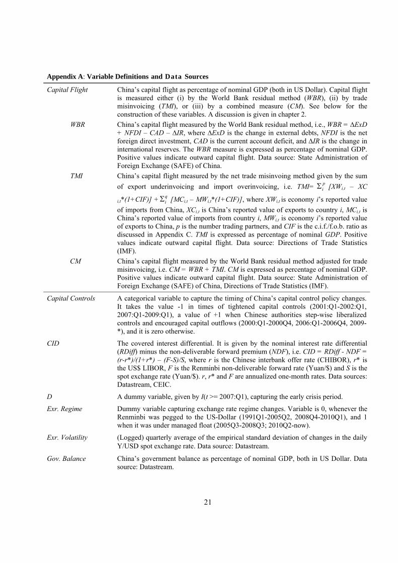
Appendix A: Variable Definitions and Data Sources

Capital Flight China’s capital flight as percentage of nominal GDP (both in US Dollar). Capital flight is measured either (i) by the World Bank residual method (WBR), (ii) by trade misinvoicing (TMI), or (iii) by a combined measure (CM). See below for the construction of these variables. A discussion is given in chapter 2.

WBR China’s capital flight measured by the World Bank residual method, i.e., WBR = ∆ExD + NFDI – CAD – ∆IR, where ∆ExD is the change in external debts, NFDI is the net foreign direct investment, CAD is the current account deficit, and ∆IR is the change in international reserves. The WBR measure is expressed as percentage of nominal GDP. Positive values indicate outward capital flight. Data source: State Administration of Foreign Exchange (SAFE) of China.

TMI China’s capital flight measured by the net trade misinvoing method given by the sum

of export underinvoicing and import overinvoicing, i.e. TMI= pi [XWi,t – XC

i,t*(1+CIF)] + qi [MCi,t – MWi,t*(1+CIF)], where XWi,t is economy i’s reported value

of imports from China, XCi,t is China’s reported value of exports to country i, MCi,t is China’s reported value of imports from country i, MWi,t is economy i’s reported value of exports to China, p is the number trading partners, and CIF is the c.i.f./f.o.b. ratio as discussed in Appendix C. TMI is expressed as percentage of nominal GDP. Positive values indicate outward capital flight. Data source: Directions of Trade Statistics (IMF).

CM China’s capital flight measured by the World Bank residual method adjusted for trade misinvoicing, i.e. CM = WBR + TMI. CM is expressed as percentage of nominal GDP. Positive values indicate outward capital flight. Data source: State Administration of Foreign Exchange (SAFE) of China, Directions of Trade Statistics (IMF).

Capital Controls A categorical variable to capture the timing of China’s capital control policy changes. It takes the value -1 in times of tightened capital controls (2001:Q1-2002:Q1, 2007:Q1-2009:Q1), a value of +1 when Chinese authorities step-wise liberalized controls and encouraged capital outflows (2000:Q1-2000Q4, 2006:Q1-2006Q4, 2009-*), and it is zero otherwise.

CID The covered interest differential. It is given by the nominal interest rate differential (RDiff) minus the non-deliverable forward premium (NDF), i.e. CID = RDiff - NDF = (r-r*)/(1+r*) – (F-S)/S, where r is the Chinese interbank offer rate (CHIBOR), r* is the US$ LIBOR, F is the Renminbi non-deliverable forward rate (Yuan/$) and S is the spot exchange rate (Yuan/$). r, r* and F are annualized one-month rates. Data sources: Datastream, CEIC.

D A dummy variable, given by I(t >= 2007:Q1), capturing the early crisis period.

Exr. Regime Dummy variable capturing exchange rate regime changes. Variable is 0, whenever the Renminbi was pegged to the US-Dollar (1991Q1-2005Q2, 2008Q4-2010Q1), and 1 when it was under managed float (2005Q3-2008Q3; 2010Q2-now).

Exr. Volatility (Logged) quarterly average of the empirical standard deviation of changes in the daily Y/USD spot exchange rate. Data source: Datastream.

Gov. Balance China’s government balance as percentage of nominal GDP, both in US Dollar. Data source: Datastream.

22

Inflation Diff. The difference between the Chinese and US inflation rate in percentage points. Data source: International Financial Statistics (IFS).

NDF The renminbi nondeliverable forward premium given by (F-S)/S, where F and S are nondeliverable forward and spot rates (Y/$), respectively. An NDF > 0 indicates an expected $ appreciation. Data sources: Datastream, CEIC.

Oil price Crude Oil-Brent Spot FOB U$/BBL. Data source: Datastream.

Openness China’s trade openness scaled by GDP. Openness is measured by the total value of (seasonally adjusted) imports and exports. Data source: International Financial Statistics (IFS).

Outflow Controls Chen and Qian (2015) index of China’s controls of capital outflows. A large score of the index represents a tight level of controls. Data source: Chen and Qian (2015).

Political Risk China’s Political Risk Index - a higher value means a lower level of political risk. Data source: ICRG.

RDiff Interest rate differential given by (r-r*)/(1+r*), where r is the Chinese interbank offer rate (CHIBOR), r* is the US$ LIBOR (both in annualized one-month rates) Positive values of RDiff indicate a higher nominal return on investment in China. Data sources: Datastream, CEIC.

Real GDP Growth Growth rate of China’s real GDP. Data source: International Financial Statistics (IFS).

Rel. M1 China’s Monetary Aggregate M1 relative to the US, both standardized by the countries nominal GDP. All variables in levels and national currency. Data sources: Federal Reserve Economic Data (FRED), Datastream.

Reserves China’s international reserve assets in percent of nominal GDP, both in US Dollar. Data source: International Financial Statistics (IFS).

SED A dummy variable for the semi-yearly Strategic Economic Dialogue (SED) between the US and Chinese governments, starting from December 2006 and its successor, the U.S.-China Strategic and Economic Dialogue (S&ED). The variable is set to 1 in each quarter when a meeting took place, 0 otherwise

Tariffs Tariff revenue collected from imports and exports. Expressed as percentage of total trade volume. Data source: Ministry of Finance, People’s Republic of China. 

Notes: If necessary, the time series have been seasonally adjusted. The first difference of a variable is used in the regression when the series itself is I(1).

23

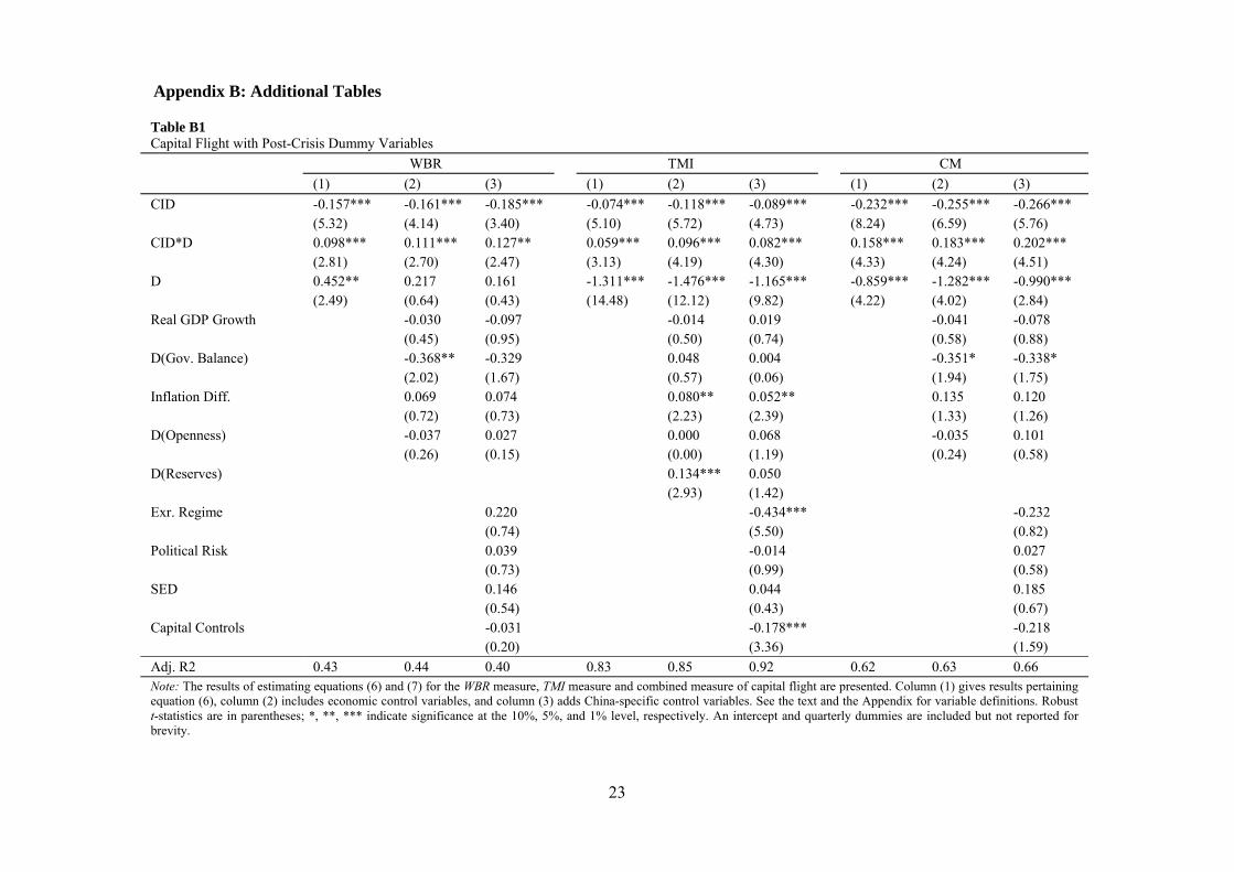
Appendix B: Additional Tables

Table B1 Capital Flight with Post-Crisis Dummy Variables

WBR TMI CM

(1) (2) (3) (1) (2) (3) (1) (2) (3)

CID -0.157*** -0.161*** -0.185*** -0.074*** -0.118*** -0.089*** -0.232*** -0.255*** -0.266*** (5.32) (4.14) (3.40) (5.10) (5.72) (4.73) (8.24) (6.59) (5.76) CID*D 0.098*** 0.111*** 0.127** 0.059*** 0.096*** 0.082*** 0.158*** 0.183*** 0.202*** (2.81) (2.70) (2.47) (3.13) (4.19) (4.30) (4.33) (4.24) (4.51) D 0.452** 0.217 0.161 -1.311*** -1.476*** -1.165*** -0.859*** -1.282*** -0.990*** (2.49) (0.64) (0.43) (14.48) (12.12) (9.82) (4.22) (4.02) (2.84) Real GDP Growth -0.030 -0.097 -0.014 0.019 -0.041 -0.078 (0.45) (0.95) (0.50) (0.74) (0.58) (0.88) D(Gov. Balance) -0.368** -0.329 0.048 0.004 -0.351* -0.338* (2.02) (1.67) (0.57) (0.06) (1.94) (1.75) Inflation Diff. 0.069 0.074 0.080** 0.052** 0.135 0.120 (0.72) (0.73) (2.23) (2.39) (1.33) (1.26) D(Openness) -0.037 0.027 0.000 0.068 -0.035 0.101 (0.26) (0.15) (0.00) (1.19) (0.24) (0.58) D(Reserves) 0.134*** 0.050 (2.93) (1.42) Exr. Regime 0.220 -0.434*** -0.232 (0.74) (5.50) (0.82) Political Risk 0.039 -0.014 0.027 (0.73) (0.99) (0.58) SED 0.146 0.044 0.185 (0.54) (0.43) (0.67) Capital Controls -0.031 -0.178*** -0.218 (0.20) (3.36) (1.59)

Adj. R2 0.43 0.44 0.40 0.83 0.85 0.92 0.62 0.63 0.66 Note: The results of estimating equations (6) and (7) for the WBR measure, TMI measure and combined measure of capital flight are presented. Column (1) gives results pertaining equation (6), column (2) includes economic control variables, and column (3) adds China-specific control variables. See the text and the Appendix for variable definitions. Robust t-statistics are in parentheses; *, **, *** indicate significance at the 10%, 5%, and 1% level, respectively. An intercept and quarterly dummies are included but not reported for brevity.

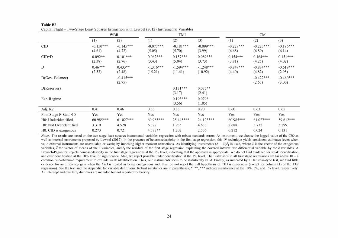
24

Table B2 Capital Flight – Two-Stage Least Squares Estimation with Lewbel (2012) Instrumental Variables

WBR TMI CM

(1) (2) (1) (2) (3) (1) (2) (3)

CID -0.150*** -0.145*** -0.077*** -0.181*** -0.099*** -0.228*** -0.223*** -0.196*** (4.61) (4.72) (5.05) (5.70) (3.99) (6.68) (6.89) (6.14)

CID*D 0.092** 0.101*** 0.062*** 0.157*** 0.089*** 0.154*** 0.164*** 0.151*** (2.38) (2.76) (3.43) (5.04) (3.73) (3.81) (4.25) (4.02)

D 0.467** 0.433** -1.316*** -1.594*** -1.248*** -0.849*** -0.884*** -0.619*** (2.53) (2.48) (15.21) (11.41) (10.92) (4.40) (4.82) (2.95)

D(Gov. Balance) -0.415*** -0.422*** -0.460*** (2.75) (2.67) (3.00)

D(Reserves) 0.131*** 0.075** (3.17) (2.41)

Exr. Regime 0.193*** 0.079* (3.56) (1.85)

Adj. R2 0.41 0.46 0.83 0.83 0.90 0.60 0.63 0.65

First Stage F-Stat >10 Yes Yes Yes Yes Yes Yes Yes Yes H0: Underidentified 60.985*** 61.027*** 60.985*** 25.445*** 24.123*** 60.985*** 61.027*** 59.612*** H0: Not Overidentified 3.319 4.528 6.322 1.935 4.633 2.688 3.732 3.299 H0: CID is exogenous 0.273 0.721 4.577** 1.202 2.556 0.212 0.024 0.131 Notes: The results are based on the two-stage-least squares instrumental variables regression with robust standards errors. As instrument, we choose the lagged value of the CID as well as internal instruments proposed by Lewbel (2012). In the presence of heteroscedasticity in the first stage regression, this IV technique yields consistent estimates (even when valid external instruments are unavailable or weak) by imposing higher moment restrictions. As identifying instruments ̅ ̂ is used, where is the vector of the exogenous variables, ̅ the vector of means of the variables, and ̂ the residual of the first stage regression explaining the covered interest rate differential variable by the variables. A Breusch-Pagan test rejects homoscedasticity in the first stage regressions at the 1% level; indicating that the approach is appropriate. We do not find evidence for weak identification and overidentification at the 10% level of significance. Also, we reject possible underidentification at the 1% level. The F-statistics in all first stage regressions are far above 10 – a common rule-of-thumb requirement to exclude weak identification. Thus, our instruments seem to be statistically valid. Finally, as indicated by a Hausman-type test, we find little evidence for an efficiency gain when the CID is treated as being endogenous and, thus, do not reject the null hypothesis of CID is exogenous (except for column (1) of the TMI regression). See the text and the Appendix for variable definitions. Robust t-statistics are in parentheses; *, **, *** indicate significance at the 10%, 5%, and 1% level, respectively. An intercept and quarterly dummies are included but not reported for brevity.

25

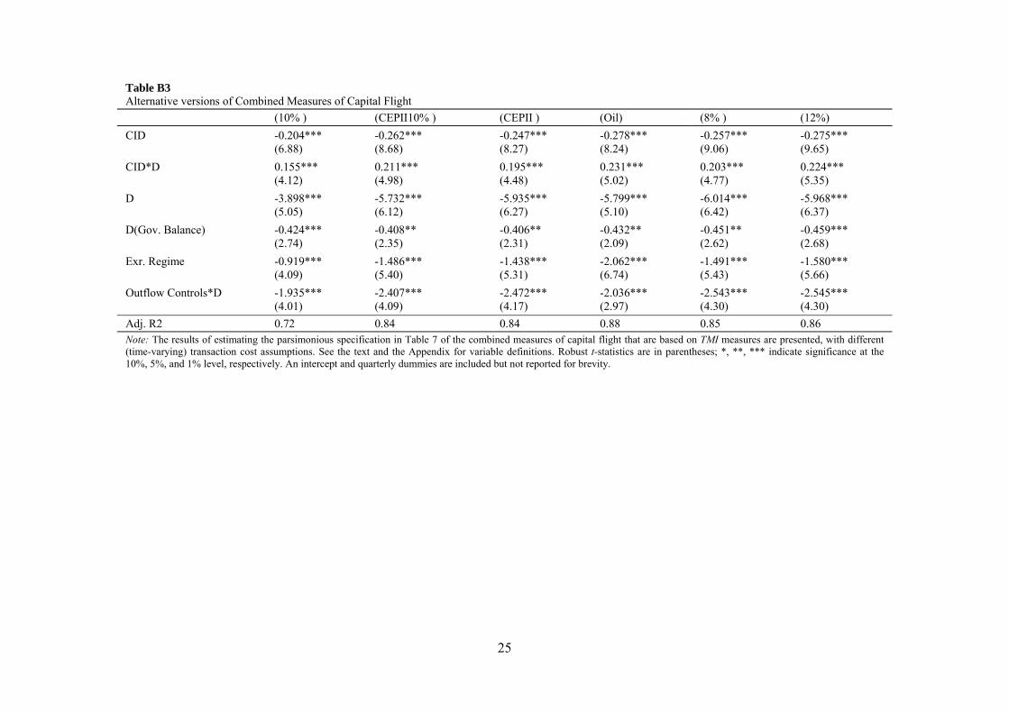
Table B3 Alternative versions of Combined Measures of Capital Flight

(10% ) (CEPII10% ) (CEPII ) (Oil) (8% ) (12%)

CID -0.204*** -0.262*** -0.247*** -0.278*** -0.257*** -0.275*** (6.88) (8.68) (8.27) (8.24) (9.06) (9.65)

CID*D 0.155*** 0.211*** 0.195*** 0.231*** 0.203*** 0.224*** (4.12) (4.98) (4.48) (5.02) (4.77) (5.35)

D -3.898*** -5.732*** -5.935*** -5.799*** -6.014*** -5.968*** (5.05) (6.12) (6.27) (5.10) (6.42) (6.37)

D(Gov. Balance) -0.424*** -0.408** -0.406** -0.432** -0.451** -0.459*** (2.74) (2.35) (2.31) (2.09) (2.62) (2.68)

Exr. Regime -0.919*** -1.486*** -1.438*** -2.062*** -1.491*** -1.580*** (4.09) (5.40) (5.31) (6.74) (5.43) (5.66)

Outflow Controls*D -1.935*** -2.407*** -2.472*** -2.036*** -2.543*** -2.545*** (4.01) (4.09) (4.17) (2.97) (4.30) (4.30)

Adj. R2 0.72 0.84 0.84 0.88 0.85 0.86 Note: The results of estimating the parsimonious specification in Table 7 of the combined measures of capital flight that are based on TMI measures are presented, with different (time-varying) transaction cost assumptions. See the text and the Appendix for variable definitions. Robust t-statistics are in parentheses; *, **, *** indicate significance at the 10%, 5%, and 1% level, respectively. An intercept and quarterly dummies are included but not reported for brevity.

26

Appendix C: Alternative Measures of Trade Misinvoicing

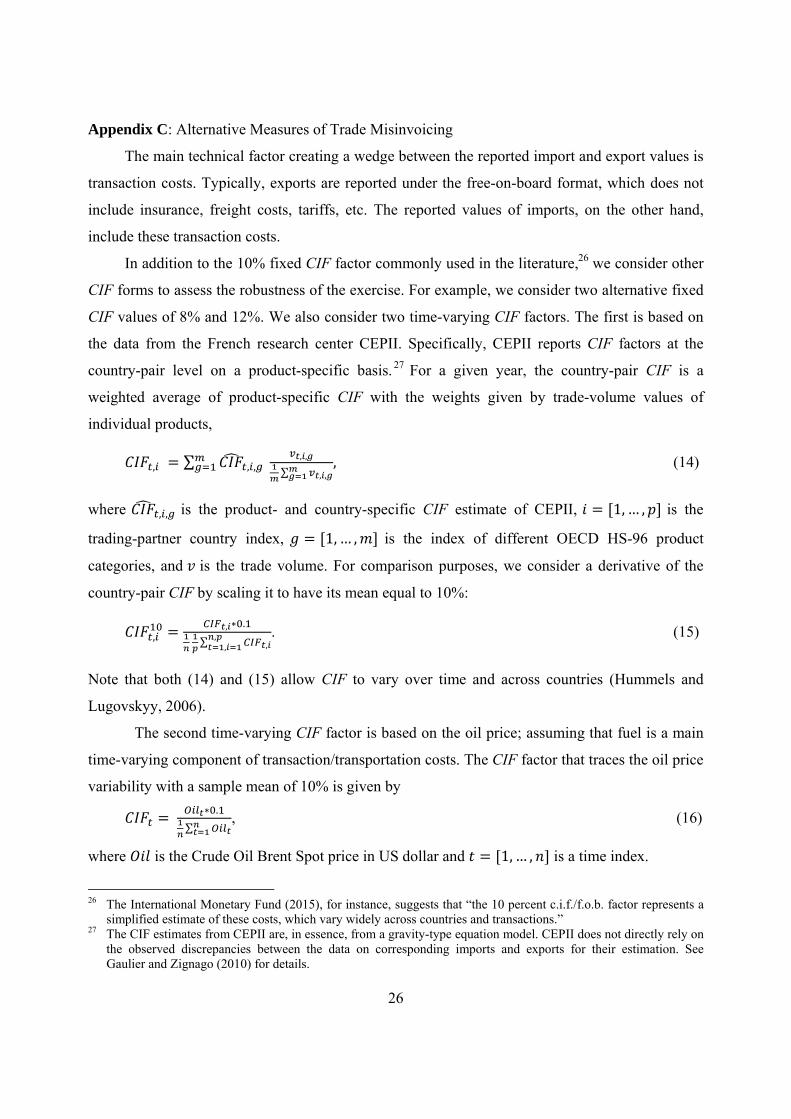
The main technical factor creating a wedge between the reported import and export values is

transaction costs. Typically, exports are reported under the free-on-board format, which does not

include insurance, freight costs, tariffs, etc. The reported values of imports, on the other hand,

include these transaction costs.

In addition to the 10% fixed CIF factor commonly used in the literature,26 we consider other

CIF forms to assess the robustness of the exercise. For example, we consider two alternative fixed

CIF values of 8% and 12%. We also consider two time-varying CIF factors. The first is based on

the data from the French research center CEPII. Specifically, CEPII reports CIF factors at the

country-pair level on a product-specific basis. 27 For a given year, the country-pair CIF is a

weighted average of product-specific CIF with the weights given by trade-volume values of

individual products,

, ∑ , , , ,

∑ , ,, (14)

where , , is the product- and country-specific CIF estimate of CEPII, 1,… , is the

trading-partner country index, 1,… , is the index of different OECD HS-96 product

categories, and is the trade volume. For comparison purposes, we consider a derivative of the

country-pair CIF by scaling it to have its mean equal to 10%:

,, ∗ .

∑ ,,,

. (15)

Note that both (14) and (15) allow CIF to vary over time and across countries (Hummels and

Lugovskyy, 2006).

The second time-varying CIF factor is based on the oil price; assuming that fuel is a main

time-varying component of transaction/transportation costs. The CIF factor that traces the oil price

variability with a sample mean of 10% is given by

∗ .∑

, (16)

where is the Crude Oil Brent Spot price in US dollar and 1,… , is a time index.

26 The International Monetary Fund (2015), for instance, suggests that “the 10 percent c.i.f./f.o.b. factor represents a

simplified estimate of these costs, which vary widely across countries and transactions.” 27 The CIF estimates from CEPII are, in essence, from a gravity-type equation model. CEPII does not directly rely on

the observed discrepancies between the data on corresponding imports and exports for their estimation. See Gaulier and Zignago (2010) for details.

27

References

Aizenman, J., Cheung, Y.-W., Ito, H., 2015. International reserves before and after the global crisis: Is there no end to hoarding? J. Int. Money Financ. 52, 102–126. doi:10.1016/j.jimonfin.2014.11.015

Bayoumi, T., Ohnsorge, F., 2013. Do Inflows or Outflows Dominate? Global Implications of Capital Account Liberalization in China, IMF Working Papers, No. 13/189. doi:10.5089/9781475532159.001

Beja, E.L., 2008. Estimating Trade Mis-invoicing from China: 2000–2005. China World Econ. 16, 82–92. doi:10.1111/j.1749-124X.2008.00108.x

Bhagwati, J.N., 1981. Alternative theories of illegal trade : Economic consequences and statistical detection. Weltwirtsch. Arch. 117(3), 409–427. doi:10.1007/BF02706100

Bhagwati, J.N., 1964. On the underinvoicing of imports. Bull. Oxford Univ. Inst. Econ. Stat. 27(4), 389–397. doi:10.1111/j.1468-0084.1964.mp27004007.x

Boyce, J.K., 1992. The revolving door? External debt and capital flight: A Philippine case study. World Dev. 20(3), 335–349. doi:10.1016/0305-750X(92)90028-T

Boyce, J.K., Ndikumana, L., 2001. Is Africa a Net Creditor? New Estimates of Capital Flight from Severely Indebted Sub-Saharan African Countries, 1970-96. J. Dev. Stud. 38(2), 27–56. doi:10.1080/00220380412331322261

Cardoso, E. a., Dornbusch, R., 1989. Foreign private capital flows, in: Handbook of Development Economics. pp. 1387–1439. doi:10.1016/S1573-4471(89)02013-9

Cerra, V., Rishi, M., Saxena, S.C., 2008. Robbing the Riches: Capital Flight, Institutions and Debt. J. Dev. Stud. 44(8), 1190–1213. doi:10.1080/00220380802242453

Chen, J., 2013. Crisis, Capital Controls, and Covered Interest Parity: Evidence from China in Transformation, in: Cheung, Y.-W., De Haan, J. (Eds.), The Evolving Role of China in the Global Economy. MIT Press, Chapter 11, 339-371.

Chen, J., Qian, X., 2015. Measuring the On-Going Changes in China’s Capital Flow Management: A De Jure and a Hybrid Index Data Set, HKIMR Working Paper No.11/2015. doi:10.2139/ssrn.2605303

Cheung, Y.-W., Herrala, R., 2014. China’s Capital Controls: Through the Prism of Covered Interest Differentials. Pacific Econ. Rev. 19(1), 112–134. doi:10.1111/1468-0106.12054

Cheung, Y.-W., Qian, X., 2010. Capital flight: China’s experience. Rev. Dev. Econ. 14(2), 227–247. doi:10.1111/j.1467-9361.2010.00549.x

Cheung, Y.-W., Qian, X., 2009. Empirics of China’s Outward Direct Investment. Pacific Econ. Rev. 14(3), 312-341. doi: 10.1111/j.1468-0106.2009.00451.x

Cheung, Y.-W., Qian, X., 2009. Hoarding of International Reserves: Mrs Machlup’s Wardrobe and the Joneses. Rev. Int. Econ. 17(4), 824–843. doi:10.1111/j.1467-9396.2009.00850.x

Chinn, M.D., 2013. United States, China, and the Rebalancing Debate: Misalignment, Elasticities, and the Saving-Investment Balance, in: Cheung, Y.-W., De Haan, J. (Eds.), The Evolving Role of China in the Global Economy. MIT Press, Chapter 11, 17-51.

Claessens, S., Naude, D., 1993. Recent Estimates of Capital Flight, Policy Research Working Paper Series, No. 1186, World Bank.

Collier, P., Hoeffler, A., Pattillo, C., 2001. Flight Capital as a Portfolio Choice. World Bank Econ. Rev. 15(1), 55–80. doi:10.1093/wber/15.1.55

28

Cuddington, J.T., 1987. Capital flight. Eur. Econ. Rev. 31(1-2), 382–388. doi:10.1016/0014-2921(87)90055-9

Cuddington, J.T., 1986. Capital flight: Estimates, issues, and explanations, Princeton Studies in International Finance, No. 58.

Diwan, I., 1989. Foreign debt, crowding out and capital flight. J. Int. Money Financ. 8(1), 121–136. doi:10.1016/0261-5606(89)90018-1

Dooley, M.P., 1988. Capital flight: a response to differences in financial risks. Staff Pap. Monet. Fund 422–436.

Dornbusch, R., 1984. External debt, budget deficits and disequilibrium exchange rates, NBER Working Papers, No. 1336.

Dornbusch, R., Kuenzler, L.T., 1993. Exchange rate policy: options and issues, in: Policy Making in the Open Economy. Oxford University Press, World Bank.

Fedderke, J.., Liu, W., 2002. Modelling the determinants of capital flows and capital flight: with an application to South African data from 1960 to 1995. Econ. Model. 19(3), 419–444. doi:10.1016/S0264-9993(01)00071-2

Fernald, J.G., Babson, O., 1999. Why has China survived the Asian crisis so well? What risks remain?, International Finance Discussion Papers 633, Board of Governors of the Federal Reserve System (U.S.).

Gaulier, G., Zignago, S., 2010. Baci: international trade database at the product-level (the 1994-2007 version), CEPII Working Paper 2010-23. CEPII Working Paper 2010-23.

Gunter, F.R., 2004. Capital flight from China: 1984–2001. China Econ. Rev. 15(1), 63–85. doi:10.1016/S1043-951X(03)00026-9

Gunter, F.R., 1996. Capital flight from the People’s Republic of China: 1984–1994. China Econ. Rev. 7(1), 77–96. doi:10.1016/S1043-951X(96)90020-6

Hummels, D., Lugovskyy, V., 2006. Are matched partner trade statistics a usable measure of transportation costs? Rev. Int. Econ. 14(1), 69–86. doi:10.1111/j.1467-9396.2006.00561.x

Hung, J.H., 2008. China’s Approach to Capital Flows Since 1978: A Brief Overview, in: Cheung, Y.-W., Wong, K.-Y. (Eds.), China and Asia: Economic and Financial Interactions. Routledge, pp. 44–63.

International Monetary Fund, 2015. Direction of Trade Statistics Quarterly. Washington, DC.

International Monetary Fund, 2010. Direction of Trade Statistics Yearbook. Washington, DC.

International Monetary Fund, 1993. A Guide to Direction of Trade Statistics. Washington, DC.

Kant, C., 1996. Foreign direct investment and capital flight, Princeton Studies in International Finance, No. 80.

Kar, D., Cartwright-Smith, D., 2009. Illicit financial flows from developing countries: 2002-2006, Global Financial Integrity. Washington, DC.

Kar, D., Freitas, S., 2012. Illicit Financial Flows from China and the Role of Trade Misinvoicing, Global Financial Integrity. Washington, DC.

Kar, D., Spanjers, J., 2014. Illicit Financial Flows from Developing Countries: 2003-2012, Global Financial Integrity. Washington, DC.

Le, Q.V., Zak, P.J., 2006. Political risk and capital flight. J. Int. Money Financ. 25(2), 308–329. doi:10.1016/j.jimonfin.2005.11.001

29

Lensink, R., Hermes, N., Murinde, V., 2000. Capital flight and political risk. J. Int. Money Financ. 19(1), 73–92. doi:10.1016/S0261-5606(99)00034-0

Lewbel, A., 2012. Using Heteroscedasticity to Identify and Estimate Mismeasured and Endogenous Regressor Models. J. Bus. Econ. Stat. 30(1), 67–80. doi:10.1080/07350015.2012.643126

Ma, G., McCauley, R.N., 2008. Efficacy of China’s capital controls: evidence from price and flow data. Pacific Econ. Rev. 13(1), 104–123. doi:10.1111/j.1468-0106.2007.00392.x

Maddison, A., 2007. Chinese Economic Performance in the Long Run, 2nd ed. Organization for Economic Cooperation and Development, Paris. doi:10.1787/9789264163553-en

Mikkelsen, J.G., 1991. An econometric investigation of capital flight. Appl. Econ. 23(1), 73–85. doi:10.1080/00036849108841050

Ndikumana, L., Boyce, J.K., 2003. Public Debts and Private Assets: Explaining Capital Flight from Sub-Saharan African Countries. World Dev. 31(1), 107–130. doi:10.1016/S0305-750X(02)00181-X

Pastor, M., 1990. Capital flight from Latin America. World Dev. 18(1), 1–18. doi:10.1016/0305-750X(90)90099-J

Prasad, E.S., Wei, S.-J., 2007. The Chinese Approach to Capital Inflows: Patterns and Possible Explanations, in: Edwards, S. (Ed.), Capital Controls and Capital Flows in Emerging Economies: Policies, Practices and Consequences. University of Chicago Press, pp. 421–480. doi:10.3386/w11306

Rojas-Suarez, L., 1990. Risk and capital flight in developing countries, IMF Working Papers, No. 90/64.

Sakakibara, E., Yamakawa, S., 2003a. Regional Integration in East Asia: Challenges and Opportunities-Part I: History and Institutions, World Bank Policy Research Working Paper Series No. 3078.

Sakakibara, E., Yamakawa, S., 2003b. Regional Integration in East Asia: Challenges and Opportunities-Part II: Trade, Finance, and Integration, World Bank Policy Research Working Paper No. 3079.

Schneider, B., 2003. Measuring capital flight: estimates and interpretations, Working Paper 194, Overseas Development Institute.

UNCTAD, 2013. World Investment Prospects Survey, 2013-2015. United Nations, New York and Geneva.

UNCTAD, 2005. Prospects for foreign direct investment and the strategies of transnational corporations, 2005-2008. United Nations, New York and Geneva.

UNCTAD, 2004. Prospects for Foreign Direct Investment and the Strategies of Transnational Corporations, 2004-2007. United Nations, New York and Geneva.

World Bank, 1985. World Bank Report. World Bank, Washington, DC.

Yu, Y., 2009. The management of cross-border capital flows and macroeconomic stability in China, TWN Global Economic Series 14, Third World Network.

Zhao, Y., de Haan, J., Scholtens, B., Yang, H., 2013. The Dynamics of Hot Money in China, in: BOFIT and CityU HK Conference on “Renminbi and the Global Economy.”

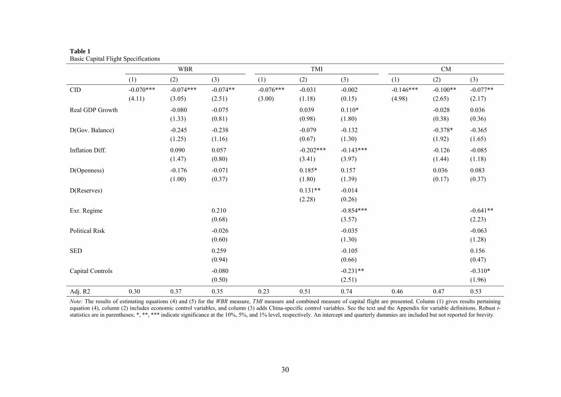
30

Table 1 Basic Capital Flight Specifications

WBR TMI CM

(1) (2) (3) (1) (2) (3) (1) (2) (3)

CID -0.070*** -0.074*** -0.074** -0.076*** -0.031 -0.002 -0.146*** -0.100** -0.077**

(4.11) (3.05) (2.51) (3.00) (1.18) (0.15) (4.98) (2.65) (2.17)

Real GDP Growth -0.080 -0.075 0.039 0.110* -0.028 0.036

(1.33) (0.81) (0.98) (1.80) (0.38) (0.36)

D(Gov. Balance) -0.245 -0.238 -0.079 -0.132 -0.378* -0.365

(1.25) (1.16) (0.67) (1.30) (1.92) (1.65)

Inflation Diff. 0.090 0.057 -0.202*** -0.143*** -0.126 -0.085

(1.47) (0.80) (3.41) (3.97) (1.44) (1.18)

D(Openness) -0.176 -0.071 0.185* 0.157 0.036 0.083

(1.00) (0.37) (1.80) (1.39) (0.17) (0.37)

D(Reserves) 0.131** -0.014

(2.28) (0.26)

Exr. Regime 0.210 -0.854*** -0.641**

(0.68) (3.57) (2.23)

Political Risk -0.026 -0.035 -0.063

(0.60) (1.30) (1.28)

SED 0.259 -0.105 0.156

(0.94) (0.66) (0.47)

Capital Controls -0.080 -0.231** -0.310*

(0.50) (2.51) (1.96)

Adj. R2 0.30 0.37 0.35 0.23 0.51 0.74 0.46 0.47 0.53

Note: The results of estimating equations (4) and (5) for the WBR measure, TMI measure and combined measure of capital flight are presented. Column (1) gives results pertaining equation (4), column (2) includes economic control variables, and column (3) adds China-specific control variables. See the text and the Appendix for variable definitions. Robust t-statistics are in parentheses; *, **, *** indicate significance at the 10%, 5%, and 1% level, respectively. An intercept and quarterly dummies are included but not reported for brevity.

31

Table 2 Capital Flight –Parsimonious Specifications of Post-Crisis CID Effects

WBR TMI CM

(1) (2) (1) (2) (3) (1) (2) (3)

CID -0.157*** -0.149*** -0.074*** -0.116*** -0.100*** -0.232*** -0.225*** -0.214*** (5.32) (4.70) (5.10) (5.94) (7.13) (8.24) (7.50) (7.23)

CID*D 0.098*** 0.105*** 0.059*** 0.097*** 0.090*** 0.158*** 0.166*** 0.167*** (2.81) (2.81) (3.13) (4.37) (5.52) (4.33) (4.26) (4.56)

D 0.452** 0.433** -1.311*** -1.447*** -1.248*** -0.859*** -0.884*** -0.630*** (2.49) (2.54) (14.48) (13.66) (11.08) (4.22) (4.82) (2.89)

D(Gov. Balance) -0.415** -0.421** -0.456*** (2.60) (2.67) (2.73)

Inflation Diff. 0.071** 0.077*** (2.36) (3.22)

D(Reserves) 0.130*** 0.084** (3.26) (2.29)

Exr. Regime -0.447*** -0.482** (4.88) (2.04)

Adj. R2 0.43 0.46 0.83 0.85 0.90 0.62 0.63 0.65

Note: The results of estimating equations (6) and (7) for the WBR measure, TMI measure and combined measure of capital flight are presented. Column (1) gives results pertaining equation (6), column (2) includes economic control variables, and column (3) adds China-specific control variables. Only the parsimonious specifications are presented. See the text and the Appendix for variable definitions. Robust t-statistics are in parentheses; *, **, *** indicate significance at the 10%, 5%, and 1% level, respectively. An intercept and quarterly dummies are included but not reported for brevity.

32

Table 3 Capital Flight – Relative Monetary Policy Effects

WBR TMI CM

(1) (2) (1) (2) (3) (1) (2) (3)

CID -0.129*** -0.128*** -0.091*** -0.122*** -0.106*** -0.220*** -0.206*** -0.206*** (3.84) (3.59) (5.77) (6.26) (7.51) (7.05) (5.99) (5.99)

CID*D 0.069 0.083* 0.077*** 0.104*** 0.097*** 0.146*** 0.159*** 0.159*** (1.65) (1.91) (4.30) (5.09) (6.42) (3.39) (3.84) (3.84)

D 0.417** 0.389** -1.283*** -1.403*** -1.216*** -0.866*** -0.641*** -0.641*** (2.10) (2.14) (16.26) (14.18) (9.60) (4.03) (2.93) (2.93)

D(Gov. Balance) -0.399** -0.451*** -0.451*** (2.62) (2.76) (2.76)

Inflation Diff. 0.059* 0.067** (1.79) (2.61)

D(Reserves) 0.113** 0.070* (2.65) (1.90)

Exr. Regime -0.442*** -0.491** -0.491** (4.36) (2.07) (2.07)

Rel. M1 -0.258 -0.234 0.169*** 0.117 0.101 -0.089 -0.086 -0.086 (1.52) (1.39) (2.86) (1.67) (1.60) (0.50) (0.49) (0.49)

Adj. R2 0.42 0.47 0.84 0.86 0.90 0.59 0.65 0.65

Note: The results of estimating equations (8) and (9) for the WBR measure, TMI measure and combined measure of capital flight are presented. Column (1) gives results pertaining equation (8), column (2) includes economic control variables, and column (3) adds China-specific control variables. Only the parsimonious specifications are presented. See the text and the Appendix for variable definitions. Robust t-statistics are in parentheses; *, **, *** indicate significance at the 10%, 5%, and 1% level, respectively. An intercept and quarterly dummies are included but not reported for brevity.

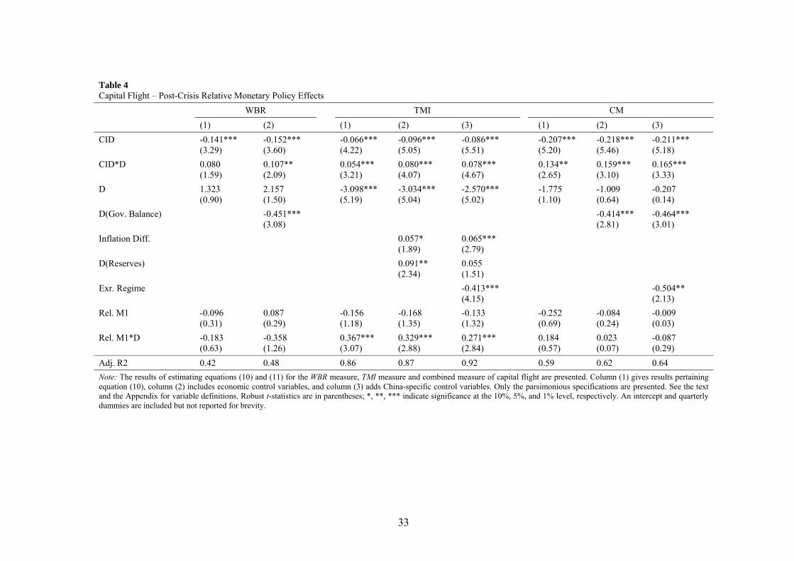
33

Table 4 Capital Flight – Post-Crisis Relative Monetary Policy Effects

WBR TMI CM

(1) (2) (1) (2) (3) (1) (2) (3)

CID -0.141*** -0.152*** -0.066*** -0.096*** -0.086*** -0.207*** -0.218*** -0.211*** (3.29) (3.60) (4.22) (5.05) (5.51) (5.20) (5.46) (5.18)

CID*D 0.080 0.107** 0.054*** 0.080*** 0.078*** 0.134** 0.159*** 0.165*** (1.59) (2.09) (3.21) (4.07) (4.67) (2.65) (3.10) (3.33)

D 1.323 2.157 -3.098*** -3.034*** -2.570*** -1.775 -1.009 -0.207 (0.90) (1.50) (5.19) (5.04) (5.02) (1.10) (0.64) (0.14)

D(Gov. Balance) -0.451*** -0.414*** -0.464*** (3.08) (2.81) (3.01)

Inflation Diff. 0.057* 0.065*** (1.89) (2.79)

D(Reserves) 0.091** 0.055 (2.34) (1.51)

Exr. Regime -0.413*** -0.504** (4.15) (2.13)

Rel. M1 -0.096 0.087 -0.156 -0.168 -0.133 -0.252 -0.084 -0.009 (0.31) (0.29) (1.18) (1.35) (1.32) (0.69) (0.24) (0.03)

Rel. M1*D -0.183 -0.358 0.367*** 0.329*** 0.271*** 0.184 0.023 -0.087 (0.63) (1.26) (3.07) (2.88) (2.84) (0.57) (0.07) (0.29)

Adj. R2 0.42 0.48 0.86 0.87 0.92 0.59 0.62 0.64

Note: The results of estimating equations (10) and (11) for the WBR measure, TMI measure and combined measure of capital flight are presented. Column (1) gives results pertaining equation (10), column (2) includes economic control variables, and column (3) adds China-specific control variables. Only the parsimonious specifications are presented. See the text and the Appendix for variable definitions. Robust t-statistics are in parentheses; *, **, *** indicate significance at the 10%, 5%, and 1% level, respectively. An intercept and quarterly dummies are included but not reported for brevity.

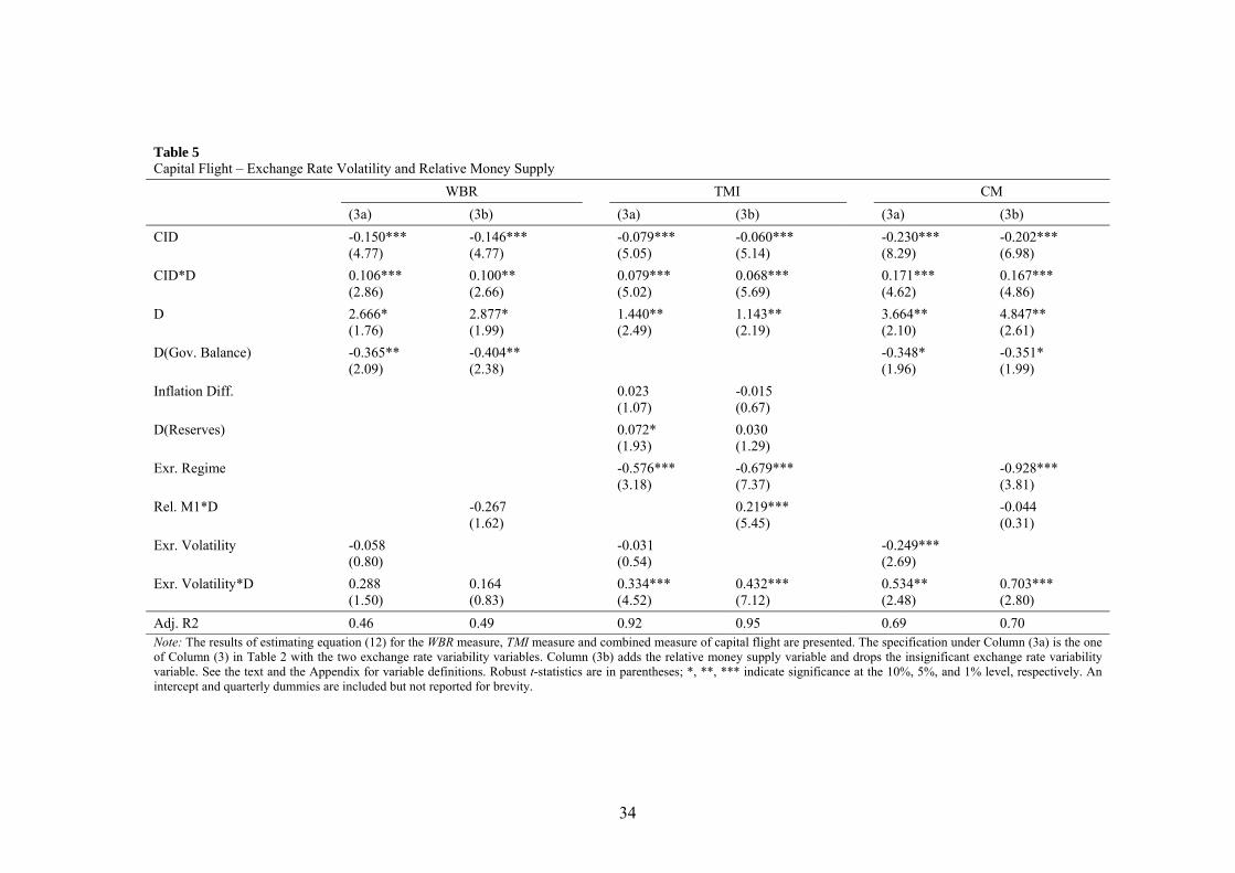
34

Table 5 Capital Flight – Exchange Rate Volatility and Relative Money Supply

WBR TMI CM

(3a) (3b) (3a) (3b) (3a) (3b)

CID -0.150*** -0.146*** -0.079*** -0.060*** -0.230*** -0.202*** (4.77) (4.77) (5.05) (5.14) (8.29) (6.98)

CID*D 0.106*** 0.100** 0.079*** 0.068*** 0.171*** 0.167*** (2.86) (2.66) (5.02) (5.69) (4.62) (4.86)

D 2.666* 2.877* 1.440** 1.143** 3.664** 4.847** (1.76) (1.99) (2.49) (2.19) (2.10) (2.61)

D(Gov. Balance) -0.365** -0.404** -0.348* -0.351* (2.09) (2.38) (1.96) (1.99)

Inflation Diff. 0.023 -0.015 (1.07) (0.67)

D(Reserves) 0.072* 0.030 (1.93) (1.29)

Exr. Regime -0.576*** -0.679*** -0.928*** (3.18) (7.37) (3.81)

Rel. M1*D -0.267 0.219*** -0.044 (1.62) (5.45) (0.31)

Exr. Volatility -0.058 -0.031 -0.249*** (0.80) (0.54) (2.69)

Exr. Volatility*D 0.288 0.164 0.334*** 0.432*** 0.534** 0.703*** (1.50) (0.83) (4.52) (7.12) (2.48) (2.80)

Adj. R2 0.46 0.49 0.92 0.95 0.69 0.70 Note: The results of estimating equation (12) for the WBR measure, TMI measure and combined measure of capital flight are presented. The specification under Column (3a) is the one of Column (3) in Table 2 with the two exchange rate variability variables. Column (3b) adds the relative money supply variable and drops the insignificant exchange rate variability variable. See the text and the Appendix for variable definitions. Robust t-statistics are in parentheses; *, **, *** indicate significance at the 10%, 5%, and 1% level, respectively. An intercept and quarterly dummies are included but not reported for brevity.

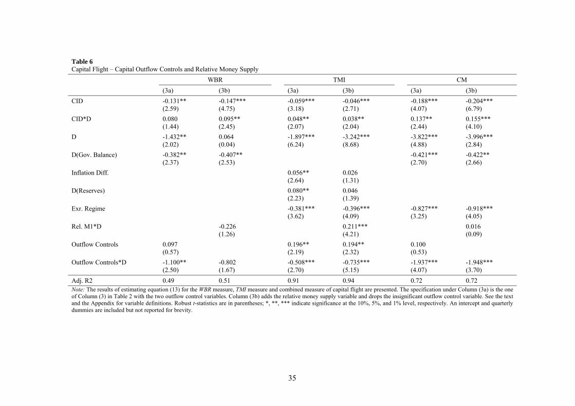
35

Table 6 Capital Flight – Capital Outflow Controls and Relative Money Supply

WBR TMI CM

(3a) (3b) (3a) (3b) (3a) (3b)

CID -0.131** -0.147*** -0.059*** -0.046*** -0.188*** -0.204*** (2.59) (4.75) (3.18) (2.71) (4.07) (6.79)

CID*D 0.080 0.095** 0.048** 0.038** 0.137** 0.155*** (1.44) (2.45) (2.07) (2.04) (2.44) (4.10)

D -1.432** 0.064 -1.897*** -3.242*** -3.822*** -3.996*** (2.02) (0.04) (6.24) (8.68) (4.88) (2.84)

D(Gov. Balance) -0.382** -0.407** -0.421*** -0.422** (2.37) (2.53) (2.70) (2.66)

Inflation Diff. 0.056** 0.026 (2.64) (1.31)

D(Reserves) 0.080** 0.046 (2.23) (1.39)

Exr. Regime -0.381*** -0.396*** -0.827*** -0.918*** (3.62) (4.09) (3.25) (4.05)

Rel. M1*D -0.226 0.211*** 0.016 (1.26) (4.21) (0.09)

Outflow Controls 0.097 0.196** 0.194** 0.100 (0.57) (2.19) (2.32) (0.53)

Outflow Controls*D -1.100** -0.802 -0.508*** -0.735*** -1.937*** -1.948*** (2.50) (1.67) (2.70) (5.15) (4.07) (3.70)

Adj. R2 0.49 0.51 0.91 0.94 0.72 0.72 Note: The results of estimating equation (13) for the WBR measure, TMI measure and combined measure of capital flight are presented. The specification under Column (3a) is the one of Column (3) in Table 2 with the two outflow control variables. Column (3b) adds the relative money supply variable and drops the insignificant outflow control variable. See the text and the Appendix for variable definitions. Robust t-statistics are in parentheses; *, **, *** indicate significance at the 10%, 5%, and 1% level, respectively. An intercept and quarterly dummies are included but not reported for brevity.

36

Table 7 Capital Flight - Relative Money Supply, Exchange Rate Volatility, and Capital Controls

WBR TMI CM

(3a) (3b) (3a) (3b) (3a) (3b)

CID -0.115 -0.149*** -0.035 -0.059*** -0.151** -0.204*** (1.45) (4.69) (1.36) (6.44) (2.11) (6.88)

CID*D 0.059 0.098** 0.036 0.065*** 0.105 0.155*** (0.72) (2.57) (1.38) (6.26) (1.39) (4.12)

D -0.675 -1.381* -0.387 0.947* -0.716 -3.898*** (0.20) (1.99) (0.35) (1.96) (0.20) (5.05)

D(Gov. Balance) -0.474*** -0.382** -0.414** -0.424*** (2.73) (2.39) (2.52) (2.74)

Inflation Diff. -0.008 (0.31)

D(Reserves) 0.037 (1.42)

Exr. Regime -0.542*** -0.685*** -1.182** -0.919*** (4.16) (7.57) (2.33) (4.09)

Rel. M1 0.338 0.005 0.283 (0.86) (0.05) (0.74)

Rel. M1*D -0.433 0.253*** 0.221*** -0.051 (1.38) (3.22) (5.60) (0.16)

Exr. Volatility -0.013 -0.002 0.109 (0.14) (0.04) (0.84)

Exr. Volatility*D -0.150 0.313*** 0.413*** 0.304 (0.53) (3.71) (7.74) (0.95)

Outflow Controls 0.216 0.149 0.245 (0.87) (1.46) (1.01)

Outflow Controls*D -1.269* -1.003** -0.308 -1.465* -1.935*** (1.72) (2.48) (1.47) (1.79) (4.01)

Adj. R2 0.48 0.49 0.95 0.95 0.72 0.72 Note: The results of estimating the combined effects of Relative Money Supply, Exchange Rate Volatility, and Capital Controls for the WBR measure, TMI measure and combined measure of capital flight are presented. The specification under Column (3a) is the one of Column (3) in Table 2 with the Relative Money Supply, Exchange Rate Volatility, and Capital Control variables. Column (3b) presents only the significant variables. See the text and the Appendix for variable definitions. Robust t-statistics are in parentheses; *, **, *** indicate significance at the 10%, 5%, and 1% level, respectively. An intercept and quarterly dummies are included but not reported for brevity.

37

Table 8 Alternative Measures of Trade Misinvoicing

(10% ) (CEPII10% ) (CEPII ) (Oil) (8% ) (12%)

CID -0.059*** -0.053*** -0.038*** -0.067*** -0.050*** -0.068*** (6.44) (6.06) (4.10) (5.95) (5.30) (7.54)

CID*D 0.065*** 0.061*** 0.047*** 0.080*** 0.055*** 0.075*** (6.26) (5.66) (4.21) (5.15) (5.32) (7.09)

D 0.947* 0.828* 0.653 0.021 0.786* 1.109** (1.96) (1.68) (1.26) (0.02) (1.68) (2.20)

Exr. Regime -0.685*** -0.655*** -0.596*** -1.318*** -0.634*** -0.736*** (7.57) (7.44) (6.78) (10.34) (7.17) (7.89)

Rel. M1*D 0.221*** 0.197*** 0.252*** 0.278*** 0.249*** 0.194*** (5.60) (4.09) (4.93) (2.85) (6.26) (4.87)

Exr. Volatility*D 0.413*** 0.377*** 0.402*** 0.414*** 0.412*** 0.413*** (7.74) (6.18) (6.14) (3.77) (7.92) (7.41)

Adj. R2 0.95 0.93 0.93 0.94 0.94 0.95 Note: The results of estimating the parsimonious specification in Table 7 of the TMI measure of capital flight, constructed under various transaction cost assumptions, are presented. See the text and the Appendix for variable definitions. Robust t-statistics are in parentheses; *, **, *** indicate significance at the 10%, 5%, and 1% level, respectively. An intercept and quarterly dummies are included but not reported for brevity.

Table 9 The role of Tariffs

TMI WBR CM

(10% ) (CEPII10% ) (CEPII ) (Oil)

CID -0.030** -0.024 -0.020 -0.034* -0.130** -0.183*** (2.10) (1.64) (1.29) (1.85) (2.34) (3.68)

CID*D 0.033** 0.028* 0.026 0.041* 0.079 0.133** (2.16) (1.70) (1.44) (1.71) (1.32) (2.28)

D 0.720 1.095** 1.090** 1.038 -0.974 -3.367** (1.52) (2.22) (2.07) (1.29) (0.86) (2.62)

D(Gov. Balance) -0.390** -0.428*** (2.44) (2.84)

Exr. Regime -0.558*** -0.502*** -0.487*** -1.108*** -0.830*** (5.90) (5.12) (4.79) (6.97) (3.44)

Rel. M1*D 0.233*** 0.199*** 0.249*** 0.267*** (6.15) (4.38) (5.16) (3.07)

Exr. Volatility*D 0.357*** 0.307*** 0.350*** 0.314*** (7.02) (4.79) (5.01) (2.81)

Outflow Controls*D -1.003** -1.839*** (2.42) (3.82)

Tariffs 0.344** 0.342** 0.212 0.387** 0.195 0.235 (2.43) (2.54) (1.53) (2.16) (0.49) (0.61)

Tariffs*D -0.157 -0.708* -0.743* -1.601** -0.319 -0.303 (0.45) (1.81) (1.74) (2.23) (0.31) (0.28)

Adj. R2 0.95 0.94 0.93 0.94 0.47 0.71 Note: The results of estimating the tariff revenue effect are presented. The three parsimonious specifications in Table 7 and those of the TMI measure allowing for time-varying transaction costs are considered. See the text and the Appendix for variable definitions. Robust t-statistics are in parentheses; *, **, *** indicate significance at the 10%, 5%, and 1% level, respectively. An intercept and quarterly dummies are included but not reported for brevity.

38

Table 10 The Individual Roles of Interest Rate Differential and Exchange Rate Premium

TMI WBR CM

(10% ) (CEPII10% ) (CEPII ) (Oil)

RDiff -0.065*** -0.070*** -0.066*** -0.044 -0.069 -0.129* (2.74) (3.44) (3.29) (1.59) (0.96) (1.76)

NDF 0.059*** 0.047*** 0.027** 0.082*** 0.184*** 0.245*** (5.16) (4.27) (2.56) (5.55) (6.39) (7.99)

RDiff*D 0.065* 0.029 0.005 -0.073 0.044 0.048 (1.79) (0.91) (0.16) (1.36) (0.43) (0.44)

NDF*D -0.066*** -0.059*** -0.040*** -0.097*** -0.130*** -0.193*** (5.32) (4.57) (3.26) (5.49) (3.61) (5.34)

D 1.051* 1.549** 1.746*** 0.981 -1.518** -3.586*** (1.74) (2.47) (2.89) (1.05) (2.18) (4.97)

D(Gov. Balance) -0.694*** -0.685*** -0.652*** -1.186*** -0.664** (6.23) (6.03) (5.88) (7.50) (2.57)

Exr. Regime 0.210*** 0.096* 0.107* 0.028 (4.53) (1.77) (1.96) (0.30)

Rel. M1*D 0.417*** 0.391*** 0.428*** 0.355*** (6.65) (5.68) (6.24) (3.09)

Exr. Volatility*D -0.367** -0.411** (2.26) (2.59)

Outflow Controls*D -0.998** -1.674*** (2.32) (3.65)

Adj. R2 0.95 0.94 0.94 0.95 0.50 0.72

Note: The results of estimating the individual roles of interest rate differential and exchange rate premium are presented. The specifications are those considered in Table 9. See the text and the Appendix for variable definitions. Robust t-statistics are in parentheses; *, **, *** indicate significance at the 10%, 5%, and 1% level, respectively. An intercept and quarterly dummies are included but not reported for brevity.

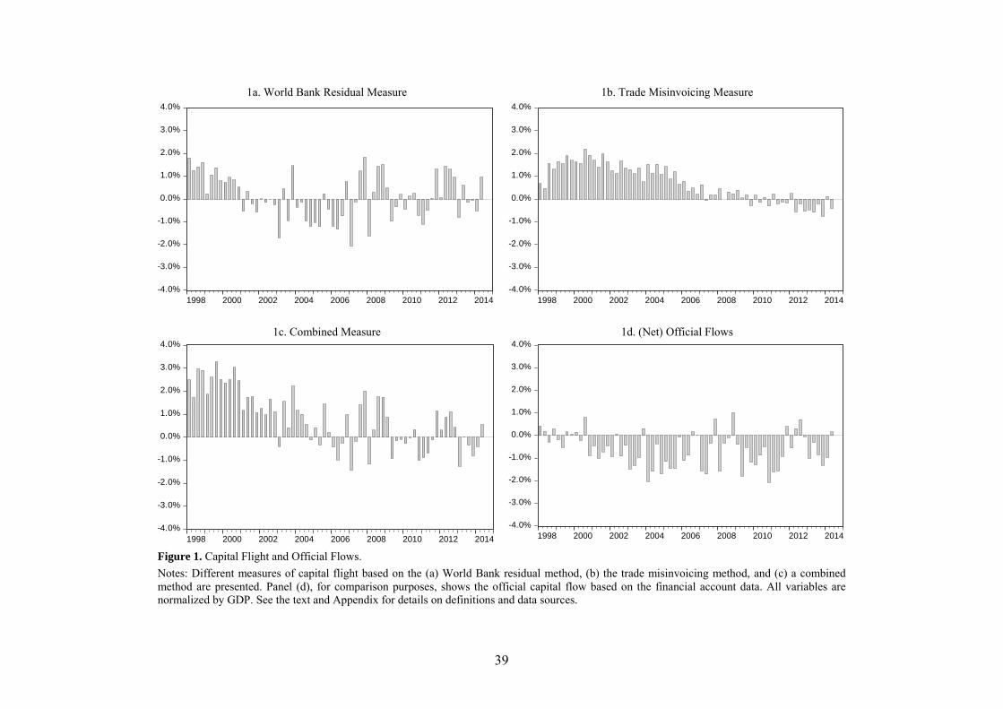
39

1a. World Bank Residual Measure

1b. Trade Misinvoicing Measure

1c. Combined Measure 1d. (Net) Official Flows

-4.0%

-3.0%

-2.0%

-1.0%

0.0%

1.0%

2.0%

3.0%

4.0%

1998 2000 2002 2004 2006 2008 2010 2012 2014

Figure 1. Capital Flight and Official Flows.

Notes: Different measures of capital flight based on the (a) World Bank residual method, (b) the trade misinvoicing method, and (c) a combined method are presented. Panel (d), for comparison purposes, shows the official capital flow based on the financial account data. All variables are normalized by GDP. See the text and Appendix for details on definitions and data sources.

-4.0%

-3.0%

-2.0%

-1.0%

0.0%

1.0%

2.0%

3.0%

4.0%

1998 2000 2002 2004 2006 2008 2010 2012 2014-4.0%

-3.0%

-2.0%

-1.0%

0.0%

1.0%

2.0%

3.0%

4.0%

1998 2000 2002 2004 2006 2008 2010 2012 2014

-4.0%

-3.0%

-2.0%

-1.0%

0.0%

1.0%

2.0%

3.0%

4.0%

1998 2000 2002 2004 2006 2008 2010 2012 2014