77th EAGE Conference & Exhibition 2015 IFEMA Madrid, Spain, 1-4 June 2015

1-4 June 2015 | IFEMA Madrid

We P3 09Robust Simultaneous Time-lapse Full-waveformInversion with Total-variation Regularization ofModel DifferenceM. Maharramov* (Stanford University) & B. Biondi (Stanford University)

SUMMARYWe present a technique for reconstructing production-induced subsurface velocity model changes fromtime-lapse seismic data using full-waveform inversion (FWI). The technique is based on simultaneouslyinverting multiple survey vintages with model-difference regularization using the total-variation (TV)seminorm. We compare the new TV-regularized time-lapse FWI with the joint time-lapse FWI from ourearlier work and the popular sequential difference method. We tested the proposed method on syntheticdatasets that exhibit survey repeatability issues. The results demonstrate advantages of the proposed TV-regularized simultaneous inversion over alternative methods for recovering production-induced velocitychanges, achieved by preserving sharp contrasts and reducing oscillatory artifacts.

77th EAGE Conference & Exhibition 2015 IFEMA Madrid, Spain, 1-4 June 2015

1-4 June 2015 | IFEMA Madrid

Introduction

Conventional time-lapse seismic processing techniques rely on picking time displacements and changesin reflectivity amplitudes between migrated baseline and monitor images, and converting them intoimpedance changes and subsurface deformation. This approach requires a significant amount of expertinterpretation and quality control. Wave-equation image-difference tomography is a more automatic al-ternative method to recover velocity changes (Albertin et al., 2006) that allows localized target-orientedinversion of model perturbations (Maharramov and Albertin, 2007). Another alternative is based onusing the high-resolution power of the full-waveform inversion (Sirgue et al., 2010) to reconstructproduction-induced changes from wide-offset seismic acquisitions (Routh et al., 2012; Zheng et al.,2011; Asnaashari et al., 2012; Raknes et al., 2013; Maharramov and Biondi, 2014b; Yang et al., 2014).However, time-lapse FWI is sensitive to repeatability issues (Asnaashari et al., 2012), with both coherentand incoherent noise potentially masking important production-induced changes. The joint time-lapseFWI proposed in (Maharramov and Biondi, 2014b) addresses repeatability issues by joint inversion ofmultiple vintage with model-difference regularization based on the L2-norm and produced improved re-sults when compared to the conventional time-lapse FWI techniques. In this work we extend this jointinversion approach to include edge-preserving total-variation (TV) model-difference regularization (Ma-harramov and Biondi, 2014c). We show that the new method can achieve a dramatic improvement overalternative techniques by significantly reducing oscillatory artifacts in the recovered model difference,and we demonstrate this on a synthetic dataset with added noise.

Method

FWI applications in time-lapse problems seek to recover induced changes in the subsurface model usingmultiple seismic datasets from different acquisition vintages. For two surveys sufficiently separatedin time, we call such datasets (and the associated models) “baseline” and “monitor”. Time-lapse FWIcan be carried out by separately inverting the baseline and monitor models (“parallel difference”) orinverting them sequentially with, e.g., the baseline supplied as a starting model for the monitor inversion(“sequential difference”). The latter may achieve a better recovery of model differences in the presenceof incoherent noise (Asnaashari et al., 2012; Maharramov and Biondi, 2014b). Another alternative isto apply the “double-difference” method (Watanabe et al., 2004; Denli and Huang, 2009; Zheng et al.,2011; Asnaashari et al., 2012; Raknes et al., 2013). The latter approach may require significant data pre-processing and equalization (Asnaashari et al., 2012; Maharramov and Biondi, 2014b) across surveyvintages.

In all of these techniques, optimization is carried out with respect to one model at a time, albeit ofdifferent vintages at different stages of the inversion. We propose to invert the baseline and monitormodels simultaneously by solving the following optimization problem:

α‖ub(mb)−db‖22+β‖um(mm)−dm‖22+ (1)

δ‖WR(mm−mb)‖1 → min (2)

with respect to both the baseline and monitor models mb and mm. Problem (1,2) describes time-lapseFWI with the L1 regularization of a transformed model difference (2). The terms (1) correspond toseparate baseline and monitor inversions with observed data d and modeled data u. This approach differsfrom our earlier approach proposed in (Maharramov and Biondi, 2014b) by using L1-norm regularizationin (2) instead of L2-norm based regularization. In (2), R and W denote regularization and weightingoperators respectively. If R is the gradient magnitude operator

R f (x,y,z) =√

f 2x + f 2y + f 2z , (3)

then (2) becomes the “Total Variation” (TV) seminorm (Ziemer, 1989). The latter case is of partic-ular interest as minimization of the gradient L1 norm promotes “blockiness” of the model-difference,potentially reducing oscillatory artifacts (Rudin et al., 1992; Aster et al., 2012).

77th EAGE Conference & Exhibition 2015 IFEMA Madrid, Spain, 1-4 June 2015

1-4 June 2015 | IFEMA Madrid

The model difference regularization weightsWmay be obtained from prior geomechanical information.For example, a rough estimate of production-induced velocity changes can be obtained from time shifts(Hatchell and Bourne, 2005; Barkved and Kristiansen, 2005) and used to map subsurface regions ofexpected production-induced perturbation. However, successfully solving the L1-regularized problem(1,2) is less sensitive to choice of the weighting operator W. For example, we show below that theTV-regularization using (3) with W = 1 recovers non-oscillatory components of the model difference,while the L2 approach would result in either smoothing or uniform reduction of the model difference.

In addition to the fully simultaneous inversion, Maharramov and Biondi (2013, 2014b) proposed andtested a “cross-updating” technique that offers a simple but remarkably effective approximation to min-imizing the objective function (1), while obviating the difference regularization and weighting operatorsR and W. This technique consists of one standard run of the sequential difference algorithm, followedby a second run with the inverted monitor model supplied as the starting model for the second baselineinversion

mINIT →baseline inversion→monitor inversion →

baseline inversion→monitor inversion,(4)

and computing the difference of the latest inverted monitor and baseline models. Cross-updating andthe simultaneous inversion with L2-based model difference regularization yielded qualitatively similarresults within the inversion target (Maharramov and Biondi, 2014b). In this paper we compare theresults of applying the sequential difference and cross-updating against simultaneous inversion with aTV-regularized model difference (1,2,3), and demonstrate the ability of the new approach to preservesharp contrasts and reduce oscillatory artifacts.

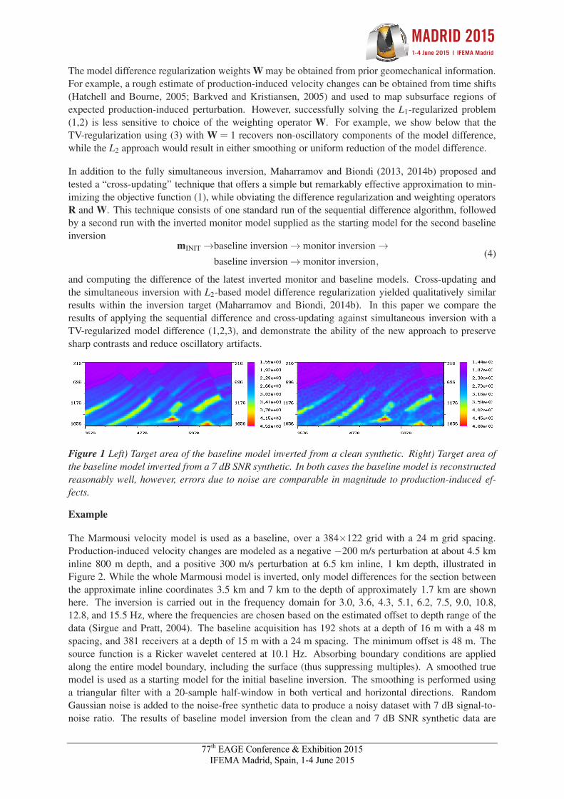
Figure 1 Left) Target area of the baseline model inverted from a clean synthetic. Right) Target area ofthe baseline model inverted from a 7 dB SNR synthetic. In both cases the baseline model is reconstructedreasonably well, however, errors due to noise are comparable in magnitude to production-induced ef-fects.

Example

The Marmousi velocity model is used as a baseline, over a 384×122 grid with a 24 m grid spacing.Production-induced velocity changes are modeled as a negative −200 m/s perturbation at about 4.5 kminline 800 m depth, and a positive 300 m/s perturbation at 6.5 km inline, 1 km depth, illustrated inFigure 2. While the whole Marmousi model is inverted, only model differences for the section betweenthe approximate inline coordinates 3.5 km and 7 km to the depth of approximately 1.7 km are shownhere. The inversion is carried out in the frequency domain for 3.0, 3.6, 4.3, 5.1, 6.2, 7.5, 9.0, 10.8,12.8, and 15.5 Hz, where the frequencies are chosen based on the estimated offset to depth range of thedata (Sirgue and Pratt, 2004). The baseline acquisition has 192 shots at a depth of 16 m with a 48 mspacing, and 381 receivers at a depth of 15 m with a 24 m spacing. The minimum offset is 48 m. Thesource function is a Ricker wavelet centered at 10.1 Hz. Absorbing boundary conditions are appliedalong the entire model boundary, including the surface (thus suppressing multiples). A smoothed truemodel is used as a starting model for the initial baseline inversion. The smoothing is performed usinga triangular filter with a 20-sample half-window in both vertical and horizontal directions. RandomGaussian noise is added to the noise-free synthetic data to produce a noisy dataset with 7 dB signal-to-noise ratio. The results of baseline model inversion from the clean and 7 dB SNR synthetic data are

77th EAGE Conference & Exhibition 2015 IFEMA Madrid, Spain, 1-4 June 2015

1-4 June 2015 | IFEMA Madrid

shown in Figure 1. The noisy monitor dataset is generated for the model perturbation of Figure 2 Left),using the same acquisition geometry and source wavelet. Results for model difference inversion from the7 dB SNR synthetic datasets using various methods are shown in Figures 2 and 3. The model-differenceregularization weightsW in (2) are set to 1 everywhere in the modeling domain. The two terms in (1) areof the same magnitude and therefore α and β are set to 1. Parameter δ is set to 10−6 but can be variedfor different acquisition source and geometry parameters. The result of the initial baseline inversion issupplied as a starting model for both mb and mm in the simultaneous inversion.

In all the inversions, up to 10 iterations of the nonlinear conjugate gradients algorithm (Nocedal andWright, 2006) are performed for each frequency. However, because the L1 component (2) of the objec-tive function is not smooth, differentiation of (3) may result in an overflow where the gradient magni-tude is very small. To avoid this, we use gradient smoothing similar to “Iteratively Re-weighted LeastSquares” (Aster et al., 2012): whenever the gradient magnitude (3) is below some threshold value ε , di-vision by (3) is substituted with division by ε . The threshold ε = 10−5 was chosen in our experiments tobe less than |Δv/v2|, with v as the baseline model velocity within the target area, and Δv as a lower boundon production-induced velocity changes. Note that alternative solution techniques such as “Bregman it-erations” (Goldstein and Osher, 2009) for TV-regularized problems can be employed in TV-regularized(time-lapse) FWI (Maharramov and Biondi, 2014a) where fixed and small ε-thresholding may adverselyimpact convergence.

Results

The results of applying iterated sequential difference (Maharramov and Biondi, 2014b) to the twodatasets are shown in Figure 2. The corresponding cross-updating and TV-regularized simultaneousinversion results are shown in Figure 3. While cross-updating demonstrates certain robustness with re-gard to uncorrelated noise in the data and computational artifacts (note the quantitative improvement ofthe recovered difference magnitudes in the left panel of Figure 3 compared with the right panel of Fig-ure 2), the TV-regularized simultaneous inversion (right panel of Figure 3) achieves a significant furtherimprovement by reducing oscillatory artifacts and honoring the blocky nature of the model difference.

Figure 2 Left) True velocity differences consist of a negative (−200 m/s) perturbation at about 4.5 kminline 800 m depth and a positive (300 m/s) perturbation at 6.5 km inline, 1 km depth. Right) Modeldifference inverted using iterated sequential difference.

Figure 3 Model difference recovered using Left) cross-updating, Right) simultaneous inversion with aTV-regularized model difference. Note the higher accuracy and stability to random noise of the TV-regularized simultaneous inversion.

77th EAGE Conference & Exhibition 2015 IFEMA Madrid, Spain, 1-4 June 2015

1-4 June 2015 | IFEMA Madrid

Conclusions

Our new TV-regularized simultaneous inversion technique is a more robust further development of pre-vious joint inversion methods. Use of the TV regularization in the simultaneous inversion allows robustrecovery of production-induced changes, and penalizes unwanted model oscillations that may mask use-ful production-induced changes.

Acknowledgements

The authors would like to thank Stewart Levin for a number of useful discussions, and the StanfordCenter for Computational Earth and Environmental Sciences for providing computing resources.

References

Albertin, U., Sava, P., Etgen, J. and Maharramov,M. [2006] Adjoint wave-equation velocity analysis. 76th AnnualInternational Meeting, SEG, Expanded Abstracts, 3345–3349.

Asnaashari, A., Brossier, R., Garambois, S., Audebert, F., Thore, P. and Virieux, J. [2012] Time-lapse imagingusing regularized FWI: A robustness study. 82nd Annual International Meeting, SEG, Expanded Abstracts,doi:10.1190/segam2012-0699.1, 1–5.

Aster, R., Borders, B. and Thurber, C. [2012] Parameter estimation and inverse problems. Elsevier.Barkved, O. and Kristiansen, T. [2005] Seismic time-lapse effects and stress changes: Examples from a compact-

ing reservoir. The Leading Edge, 24(12), 1244–1248.Denli, H. and Huang, L. [2009] Double-difference elastic waveform tomography in the time domain. 79th Annual

International Meeting, SEG, Expanded Abstracts, 2302–2306.Goldstein, T. and Osher, S. [2009] The split Bregman method for L1-regularized problems. SIAM Journal on

Imaging Sciences, 2(2), 323–343.Hatchell, P. and Bourne, S. [2005] Measuring reservoir compaction using time-lapse timeshifts. 75th Annual

International Meeting, SEG, Expanded Abstracts, 2500–2503.Maharramov, M. and Albertin, U. [2007] Localized image-difference wave equation tomography. 77th Annual

International Meeting, SEG, Expanded Abstracts, 3009–3013.Maharramov, M. and Biondi, B. [2013] Simultaneous time-lapse full waveform inversion. Stanford Exploration

Project Report, 150, 63–70.Maharramov, M. and Biondi, B. [2014a] Improved depth imaging by constrained full-waveform inversion. Stan-

ford Exploration Project Report, 155, 19–24.Maharramov,M. and Biondi, B. [2014b] Joint full-waveform inversion of time-lapse seismic data sets. 84th Annual

Meeting, SEG, Expanded Abstracts, 954–959.Maharramov, M. and Biondi, B. [2014c] Robust joint full-waveform inversion of time-lapse seismic datasets with

total-variation regularization. Stanford Exploration Project Report, 155, 199–208.Nocedal, J. and Wright, S.J. [2006] Numerical Optimization. Springer.Raknes, E., Weibull, W. and Arntsen, B. [2013] Time-lapse full waveform inversion: Synthetic and real data

examples. 83rd Annual International Meeting, SEG, Expanded Abstracts, 944–948.Routh, P., Palacharla, G., Chikichev, I. and Lazaratos, S. [2012] Full wavefield inversion of time-lapse data for im-

proved imaging and reservoir characterization. 82nd Annual International Meeting, SEG, Expanded Abstracts,doi:10.1190/segam2012-1043.1, 1–6.

Rudin, L.I., Osher, S. and Fatemi, E. [1992] Nonlinear total variation based noise removal algorithms. Physica D:Nonlinear Phenomena, 60(1-4), 259–268.

Sirgue, L., Barkved, O., Dellinger, J., Etgen, J., Albertin, U. and Kommendal, J. [2010] Full waveform inversion:The next leap forward in imaging at Valhall. First Break, 28(4), 65–70.

Sirgue, L. and Pratt, R. [2004] Efficient waveform inversion and imaging: A strategy for selecting temporalfrequencies. Geophysics, 69(1), 231–248.

Watanabe, T., Shimizu, S., Asakawa, E. and Matsuoka, T. [2004] Differential waveform tomography for time-lapse crosswell seismic data with application to gas hydrate production monitoring. 74th Annual InternationalMeeting, SEG, Expanded Abstracts, 2323–2326.

Yang, D., Malcolm, A.E. and Fehler, M.C. [2014] Time-lapse full waveform inversion and uncertainty analysiswith different survey geometries.

Zheng, Y., Barton, P. and Singh, S. [2011] Strategies for elastic full waveform inversion of time-lapse oceanbottom cable (OBC) seismic data. 81st Annual International Meeting, SEG, Expanded Abstracts, 4195–4200.

Ziemer, W.P. [1989] Weakly Differentiable Functions: Sobolev Spaces and Functions of Bounded Variation.Springer.