Waypoint GPS Post-Processing Guide

Chris Gifford

University of Kansas 2335 Irving Hill Road

Lawrence, KS 66045-7612 http://cresis.ku.edu

Technical Report CReSIS TR 141

September 9, 2008

This work was supported by a grant from the National Science Foundation

(#ANT-0424589).

1

Preface This guide presents the necessary steps to post-process GPS data recorded in the field using the Waypoint GrafNav/GrafNet Suite. It is not intended to be a comprehensive guide for the Waypoint software, rather a more concise version of how to process our own ground and aerial surveys. Images are included to help walk the user through the process. This guide can be used on old or new data, with most of the details being transparent to the user. The examples in this guide use data from actual CReSIS field seasons. Compared to our previous software, Topcon Tools, Waypoint GrafNav/GrafNet is much more flexible, efficient, and customizable. There are very few restrictions on both time and amount of data it can process. Like before, a USB hardware key is required to use the software. We have a single USB hardware key, so keep track of it at all times. Keys cost ~$4125 to replace (includes educational discount). Comprehensive support lasts free of charge until May 2009, which includes data assistance and software updates. Continuing this support costs ~$950 per year (includes educational discount), if renewed before year of service ends. Waypoint is widely known as the best post-processing software available, and is intended to last a very long time for the Center and its upcoming technology developments. It is recommended that users of this guide familiarize themselves with the software and accompanying utilities by referencing the comprehensive GrafNav/GrafNet binder and separate training manual. These support documents, together with those on Waypoint’s website, contain all the information one will need to operate the software. They also provide troubleshooting suggestions in further detail for common problems with data or for improving accuracy. During preliminary processing of our data, some of these problems were encountered. Again, this guide was created to expedite the process for CReSIS. A user of this guide should consult those manuals, as they contain a wealth of helpful information. If more assistance is required or if there are problems processing some of our data, contact Chris Gifford at cgifford@cresis.ku.edu or 785-864-7842, or David MacDonald of Waypoint Support at david.macdonald@novatel.ca or 403-730-4124 (Canada).

2

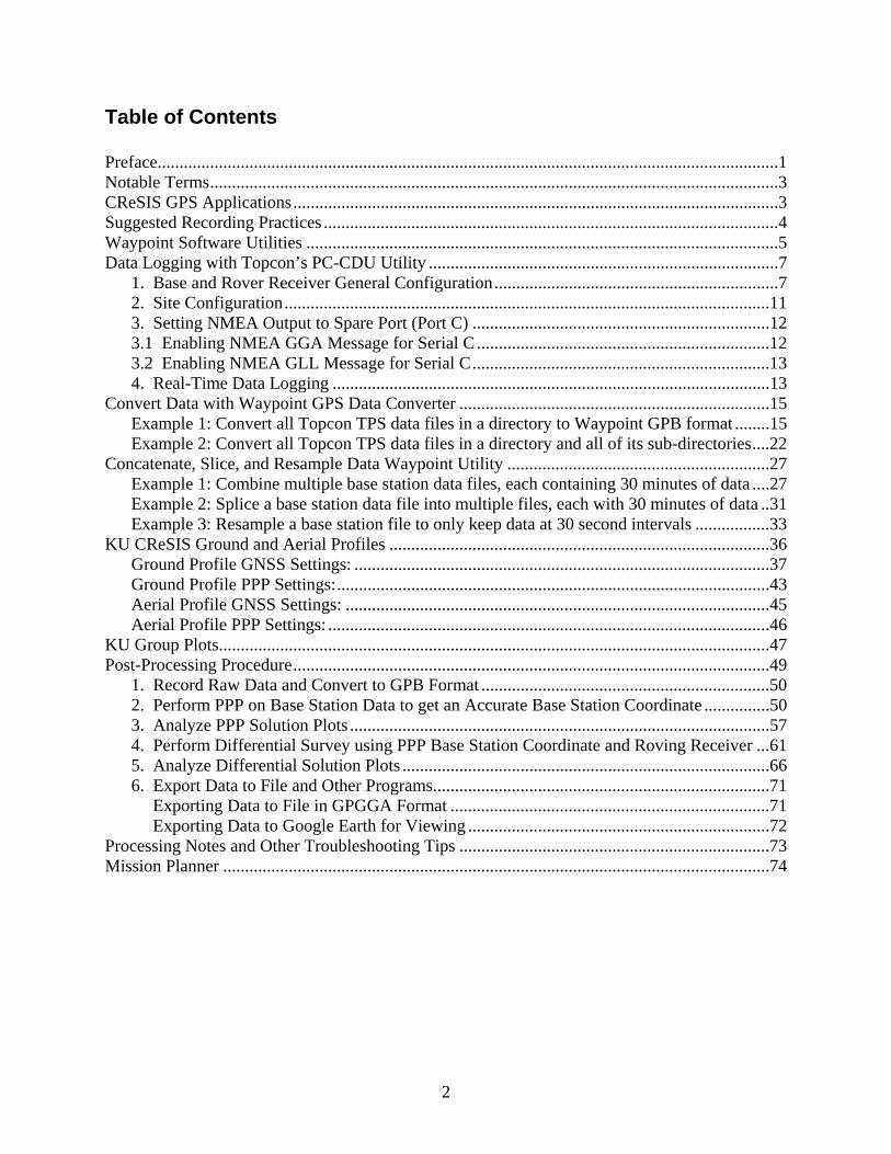
Table of Contents

Preface..............................................................................................................................................1 Notable Terms..................................................................................................................................3 CReSIS GPS Applications...............................................................................................................3 Suggested Recording Practices ........................................................................................................4 Waypoint Software Utilities ............................................................................................................5 Data Logging with Topcon’s PC-CDU Utility ................................................................................7

1. Base and Rover Receiver General Configuration.................................................................7 2. Site Configuration...............................................................................................................11 3. Setting NMEA Output to Spare Port (Port C) ....................................................................12 3.1 Enabling NMEA GGA Message for Serial C ...................................................................12 3.2 Enabling NMEA GLL Message for Serial C....................................................................13 4. Real-Time Data Logging ....................................................................................................13

Convert Data with Waypoint GPS Data Converter .......................................................................15 Example 1: Convert all Topcon TPS data files in a directory to Waypoint GPB format ........15 Example 2: Convert all Topcon TPS data files in a directory and all of its sub-directories....22

Concatenate, Slice, and Resample Data Waypoint Utility ............................................................27 Example 1: Combine multiple base station data files, each containing 30 minutes of data ....27 Example 2: Splice a base station data file into multiple files, each with 30 minutes of data ..31 Example 3: Resample a base station file to only keep data at 30 second intervals .................33

KU CReSIS Ground and Aerial Profiles .......................................................................................36 Ground Profile GNSS Settings: ...............................................................................................37 Ground Profile PPP Settings:...................................................................................................43 Aerial Profile GNSS Settings: .................................................................................................45 Aerial Profile PPP Settings: .....................................................................................................46

KU Group Plots..............................................................................................................................47 Post-Processing Procedure.............................................................................................................49

1. Record Raw Data and Convert to GPB Format ..................................................................50 2. Perform PPP on Base Station Data to get an Accurate Base Station Coordinate ...............50 3. Analyze PPP Solution Plots ................................................................................................57 4. Perform Differential Survey using PPP Base Station Coordinate and Roving Receiver ...61 5. Analyze Differential Solution Plots ....................................................................................66 6. Export Data to File and Other Programs.............................................................................71

Exporting Data to File in GPGGA Format .........................................................................71 Exporting Data to Google Earth for Viewing .....................................................................72

Processing Notes and Other Troubleshooting Tips .......................................................................73 Mission Planner .............................................................................................................................74

3

Notable Terms The following are terms that will be regularly encountered using the software and this manual. Others not listed here will be discussed throughout the guide near their examples:

• GPS: Global Position System, an American satellite constellation • GLONASS: Russian satellite constellation • GNSS: Global Navigation Satellite System, a general term consisting of available

satellites from constellations (includes GPS and GLONASS). Currently, only GPS and GLONASS are used by CReSIS in both Greenland and Antarctica.

• Base Station: Stationary receiver setup as a reference station for improving differential accuracy. Sometimes called the “Master Station” in the software.

• Roving Receiver: Moving receiver (such as that onboard the UAV or antenna sled) that typically uses a base station to improve its position accuracy offline. Also called “rover”.

• Baseline: Distance between a base station and a roving receiver. • Epoch: An instance in time, corresponding to an update rate (e.g., 1 Hz is 1 second). • Elevation Mask: Value specified in degrees which is used to reject the use of satellites

below this elevation with respect to the horizon for position calculations. Typically, the lower this mask is the more satellites that can be seen. However, satellites close to the horizon experience more atmosphere/troposphere effects and can be detrimental to position calculation.

• Kinematic: Moving. • Fixed Solution: Number of cycles (integer counts) between receiver and satellites has

been fixed. This is the more desired solution, but may not be attainable at long baselines. • Float Solution: Integer number of cycles to determine satellite distance could not be

fixed. Can be relatively close in accuracy to a fixed solution, and what we will likely see with longer baselines.

• Differential: Processing data using a static base station and a roving receiver. • PPP: Precise Point Positioning, processing of receiver data at a static base station or

without the use of an external base station if processing roving receiver data. At long baselines, this method of processing may provide better and faster solutions compared to the more typical differential processing.

• KAR / ARTK: Methods of ambiguity resolution used in the software. One can assume that we will always use ARTK, as it is faster, easier to use, and more reliable than KAR.

• WGS84 / NAD83: Datums representing reference coordinate systems. We have and will use WGS84 for CReSIS surveys. The autonomous rover also operates on WGS84 datum.

CReSIS GPS Applications CReSIS performs two main types of surveys: ground and aerial. Both survey types are typically performed with long baselines, making real-time corrections impossible, unreliable, or not needed. Ground surveys in the past and present use the Topcon equipment for both the base and the rover. Future field seasons will involve the UAV containing the roving receiver, which will record GPS data for the onboard radar using Javad equipment (receiver and aircraft antenna). In this case, the Topcon equipment (receiver and antenna) will be used to record data at the base station. See the Topcon Post-Processing Guide for more information about the Topcon

4

equipment. The post-processing portion of that guide is replaced with this guide. Topcon Tools and other processing options are no longer being used. All equipment CReSIS owns is capable of dual-frequency (L1 and L2 frequencies) recording for both GPS (American satellite constellation) and GLONASS (Russian satellite constellation). A minimum of 4 satellites are required to solve for 3 unknown variables in the software, but it is desired to have 6+ visible in case the software needs to drop satellites due to bad data from them. At the poles, this shouldn’t be much of a problem, as we have observed 7+ consistently in the field over a 24 hour period. See the “Mission Planner” section for more information about how the software can be used to plan when to fly the UAV for better satellite visibility. Of special note is the relation between the UAV’s planned banking angles during turns and the elevation mask. During turns for grid surveys, when the aircraft banks, the receiver’s antenna may lose lock on satellites. It has been suggested that a conservative elevation mask value would be equal to the bank angle of the aircraft. For example, if the UAV banks at 20 degrees, the elevation mask would be set to 20 degrees. However, in practice it is likely better to lower the elevation mask to 10. Our previous practice was to always set the elevation mask to 5. This practice can be followed for continuing experiments as well. Always use 5 when logging data. Contrary to popular belief, the recording frequency doesn’t have a profound affect on position accuracy, but rather the resolution of the position updates. It is also application-specific. For a static station, the frequency of position updates may not need to be anything less than 30 seconds (because it is stationary). For roving receivers, we typically want a finer resolution of position updates, especially if moving fast. For example, the UAV will be making a lot of movements, so we will want to have a high frequency (sub-second) update rate.

Suggested Recording Practices To keep all position data properly organized, the following suggested practices should be followed relatively closely.

• Unless disk space is limited in the field (which it never seems to be in our case), record at the highest speed possible for both base station and roving receiver. Consider this as 10 Hz, or 10 updates per second. It is always better to have more data than necessary in case we need it during processing or for future experimentation of new techniques.

• Raw data must be recorded at both the base station and roving receiver. Recording NMEA or similar strings cannot be used for post-processing. Thus, always record raw data, and use NMEA strings for time-stamping or correlating remote sensing data.

• Record raw data at the same rates for both the base station and roving receiver. • Name all base station data files “base”, followed by an ID if multiple are used. • Name all roving receiver data files “rover”, followed by an ID if multiple are used. • When the working day begins, the first task that should be done is to power on the base

station receiver and laptop and start recording data. When the working day ends, the last task should be to stop base station recording and power down base station equipment. This is to ensure that we have distinct sets of base station data for specific days, as well as base station data which overlap the roving receiver’s data. This overlap is crucial for differential processing.

5

• When the roving receiver is powered on, record data from it at all times. If it is powered off and turned back on during the same working day, create a separate data file for the second session and name it accordingly. Make note of this in a text file in that directory.

• The roving receiver can be powered on as little as 10 seconds before leaving the base if needed. It is suggested to turn it on as soon as possible. As the aircrafts we use will be near a base station during taxi, takeoff, and landing, taxi time is the minimum required recording lead-time needed for raw GPS data.

• Store all data from a day in a folder with a name indicative of the day and experiment. This includes offloading the roving receiver’s data into this location as well. This will expedite processing and keep all GPS data organized.

• Make note of anything out of the ordinary during a survey that may affect processing, including what happened and at what time. Examples are the antenna being covered during operation, a reset or powering down of recording equipment, antenna getting blown over, or the like. This may make troubleshooting much easier during processing. A text file in the day’s directory may be a good way to archive this.

• There is no need to have data files split up over a work day (e.g., a file for every 30 minutes). Store an entire work day’s data for each receiver in its own file. Files can be sampled, split, concatenated, etc with the post-processing software after acquisition. Do NOT edit raw data files manually, leave them how they are until ready for post-processing so we can let the software properly manipulate the files.

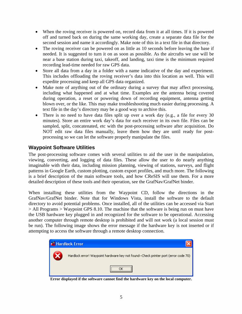
Waypoint Software Utilities The post-processing software comes with several utilities to aid the user in the manipulation, viewing, converting, and logging of data files. These allow the user to do nearly anything imaginable with their data, including mission planning, viewing of stations, surveys, and flight patterns in Google Earth, custom plotting, custom export profiles, and much more. The following is a brief description of the main software tools, and how CReSIS will use them. For a more detailed description of these tools and their operation, see the GrafNav/GrafNet binder. When installing these utilities from the Waypoint CD, follow the directions in the GrafNav/GrafNet binder. Note that for Windows Vista, install the software to the default directory to avoid potential problems. Once installed, all of the utilities can be accessed via Start > All Programs > Waypoint GPS 8.10. The machine that the software is being run on must have the USB hardware key plugged in and recognized for the software to be operational. Accessing another computer through remote desktop is prohibited and will not work (a local session must be run). The following image shows the error message if the hardware key is not inserted or if attempting to access the software through a remote desktop connection.

Error displayed if the software cannot find the hardware key on the local computer.

6

At the time of writing this guide, there were no Linux versions of the software available. Sentinel (hardware key) drivers will need updating if used with a 64-bit machine. The software utilizes at most two cores, and a dual-core machine is highly recommended for processing so forward and reverse solutions can be computed in parallel (a significant savings in time). GrafNav This is the main application that will be used for post-processing our data. Processing, viewing of all results, and exporting of processed data occur within this application. The majority of this manual involves GrafNav, as it is the main differential processing engine. We will process base stations, roving receivers, and differential projects using GrafNav. Flight lines can be viewed in Google Earth, HTML reports of plots generated, and data saved in a variety of formats. For each day of data being processed, it is expected that processing will take no longer than 15 minutes on a dual-core machine. GrafNet This is an application that can be used to process base stations with one or more nearby service stations. We may occasionally use this software to validate or determine the reliability of our differential or PPP solutions from GrafNav. For future projects which involve networks of stations (such as seismic surveying), this application may be more prominently used as it was developed for that purpose. Concatenate, Slice and Resample This tool will be used for concatenating, slicing, and resampling GPB files. It can concatenate multiple GPB files together into a single file. This feature will be used more with older data that has been previously divided into 30 minute chunks. We can also slice large files into smaller GPB files for individual processing. Resampling GPB files will come in handy when checking data for quality, by resampling data with high update rates to a smaller update interval (e.g., 10 Hz to once every 30 seconds). GPB Viewer Data viewer, allowing the user to look at raw data in GPB form. GPS Data Converter Waypoint software supports data from the majority of companies and receivers, but requires conversion of that data into Waypoint’s proprietary GPB format. This tool is used to perform this operation. Batch conversions to GPB format can be done for a single file, an entire folder, and for recursively for all folders within a selected folder. GPS Data Logger Utility to log data from nearly any available receiver, including those CReSIS uses. To eliminate the conversion process, the data logger can also directly convert and store the data in GPB format for immediate processing. This could be used as the main recording software, or as an alternative for free software utilities that came with the GPS equipment CReSIS has purchased. As we have extensively used Topcon’s PC-CDU real-time logging software, we will primarily use that until enough testing has gone into logging data with Waypoint’s Data Logger utility. Thus, always use Topcon’s PC-CDU software to log data at the base station.

7

Data Logging with Topcon’s PC-CDU Utility Before continuing, read the earlier section on “Suggested Recording Practices” to ensure that you are recording data consistently and at the proper times. Also note that as the UAV will be running a flavor of Linux, it will have a custom GPS recording application specifically written for it. Topcon’s PC-CDU software will only be used at the base station for most projects, as it requires Windows. The following provides high-level steps in order to setup Topcon equipment for a base station:

1. Setup and secure (anchor to ground) the antenna tripod. 2. Screw the Topcon Legant antenna onto the top of the tripod until it is secure. 3. Connect one end of TNC cable to the antenna and the other end of the TNC cable to the

left external connection of the black base station case. 4. Plug the power supply cord into a power source and the other end into the power

connection of the black base station case. 5. If no lights are flashing on the Topcon receiver inside the case, turn it on. 6. If only red lights are flashing, double-check the antenna connection. 7. Connect the serial cable (which may be accompanied with a USB-to-serial adapter) into

the COM or USB port of the computer that will be logging the base station’s GPS data. 8. Turn computer on and move to below set of steps to perform data logging.

The following steps can be used for general Topcon GPS receiver setup and data logging in Windows using Topcon’s PC-CDU utility, which were adapted from the Topcon Post-Processing Guide. The below example is for the Topcon equipment, as it has and will be used for the base station in the coming years. See the other Waypoint support documents for information about Waypoint’s Data Logger.

1. Check configuration of each receiver. 2. Set up site information for each receiver with a unique name for each. 3. Enable NMEA output to spare port if not already enabled. 4. Start real-time data logging 5. Collect data for receiver(s) using PC-CDU simultaneously throughout the survey process. 6. Stop real-time data logging and use Topcon Tools to post-process.

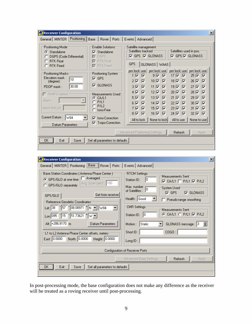
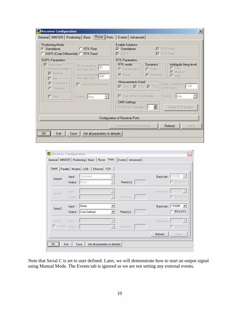
1. Base and Rover Receiver General Configuration These settings must be consistent between the rover and the base. To begin configuring the receiver, in PCCDU, click Configuration > Receiver. Now follow each tab and make any necessary changes based on what is shown in the following images.

8

Ignore the MINTER tab under Receiver Configuration, as we will not use the minter features.

5

9

In post-processing mode, the base configuration does not make any difference as the receiver will be treated as a roving receiver until post-processing.

10

Note that Serial C is set to user defined. Later, we will demonstrate how to start an output signal using Manual Mode. The Events tab is ignored as we are not setting any external events.

11

The Advanced tab features several sub-tabs for various settings. Rather than showing a picture for each, do the following. Under advanced, the following settings must be set within their respective tabs:

1) Anti-Interference: Off. 2) Multipath Reduction: Select both code and carrier boxes. 3) Loop Management: Make sure “Enable Co-Op Tracking Loop” is enabled.

All other tabs should remain unchanged.

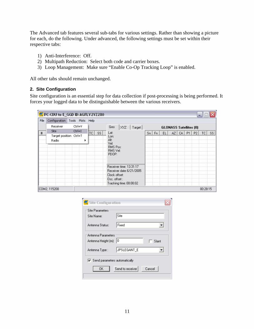
2. Site Configuration Site configuration is an essential step for data collection if post-processing is being performed. It forces your logged data to be distinguishable between the various receivers.

12

Each receiver should have a unique site configuration:

• Site Name: Give the site a unique name. When post-processing later, measurements from this site will have this assigned name. e.g. “base”, “rover_sled_1”, “rover_sled_2”, etc.

• Antenna Status: For base, select Fixed. For roving receivers, select Moving. • Antenna Height (m): The height of the antenna from the ground in meters. • Slant: Leave unchecked. • Antenna Type: Select JPSLEGANT_E. • Send parameters automatically: Checked.

Once all of the settings are finished, click the “Send to receiver” button. Then, click OK.

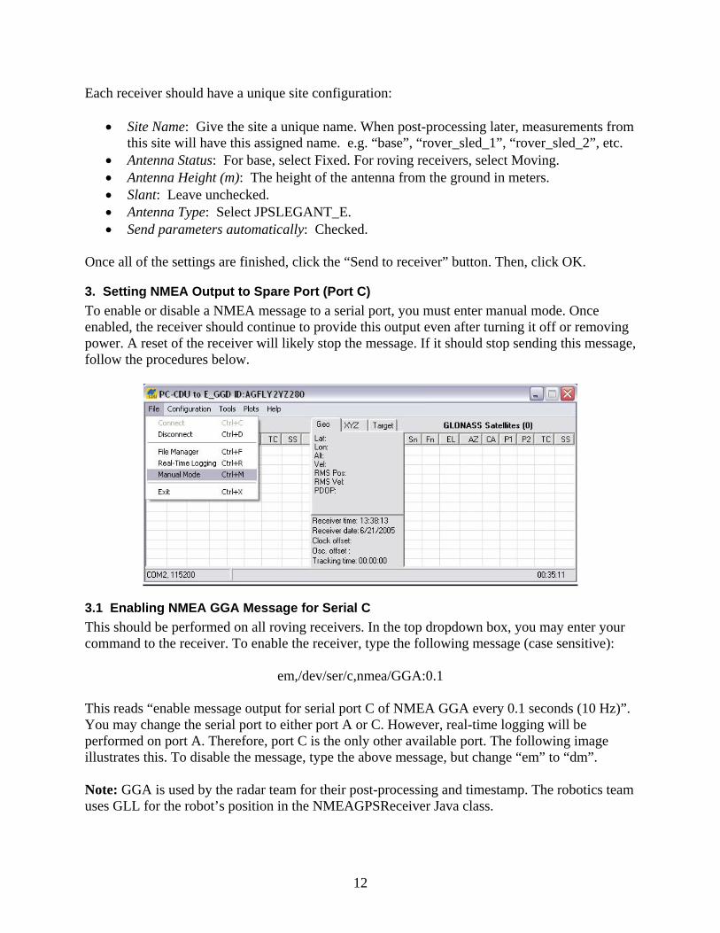
3. Setting NMEA Output to Spare Port (Port C) To enable or disable a NMEA message to a serial port, you must enter manual mode. Once enabled, the receiver should continue to provide this output even after turning it off or removing power. A reset of the receiver will likely stop the message. If it should stop sending this message, follow the procedures below.

3.1 Enabling NMEA GGA Message for Serial C This should be performed on all roving receivers. In the top dropdown box, you may enter your command to the receiver. To enable the receiver, type the following message (case sensitive):

em,/dev/ser/c,nmea/GGA:0.1 This reads “enable message output for serial port C of NMEA GGA every 0.1 seconds (10 Hz)”. You may change the serial port to either port A or C. However, real-time logging will be performed on port A. Therefore, port C is the only other available port. The following image illustrates this. To disable the message, type the above message, but change “em” to “dm”. Note: GGA is used by the radar team for their post-processing and timestamp. The robotics team uses GLL for the robot’s position in the NMEAGPSReceiver Java class.

13

3.2 Enabling NMEA GLL Message for Serial C This should be done for the robot’s GPS receiver only, unless the radar team decides to use GLL messages in the future. In the top dropdown box, you may enter your command to the receiver. To enable the receiver, type the following message (case sensitive):

em,/dev/ser/c,nmea/GLL:0.1 This reads “enable message output for serial port C of NMEA GLL every 0.1 seconds (10 Hz)”. You may change the serial port to either port A or C. However, real-time logging will be performed on port A. Therefore, port C is the only other available port. To disable the message, type the above message, but change “em” to “dm”. Note: The robot’s receiver should output both GGA and GLL. The radar team can parse only GGA and the robotics software only parses GLL.

4. Real-Time Data Logging For post-processing surveys, you will need to use the real-time data logger as the GPS receiver does not have sufficient onboard memory for large surveys.

14

Note: The elevation mask should always be set to 5 when logging raw data. The following steps can be used to setup real-time data logging. Logging must be performed simultaneously for both the roving receiver(s) and the base-station.

1. Set the name of the log file for which you want to save your raw data to. If you wish to use an existing file, when you click the Start button it will ask if you wish to overwrite or append. Create a new directory for each day of data (e.g., 121205_Monday). Set the filename to include the date (e.g., rover1_121205.tps).

2. Set the recording interval to the desired rate, which is normally 0.1 seconds (10 Hz). 3. Set the elevation mask to 5.

15

4. If you have not done so, set your site parameters as previously discussed. You may click on the “Site Parameters” button to access this window.

5. Once the logger is setup, click the Start button to begin logging raw data. When finished, click it again to stop.

Convert Data with Waypoint GPS Data Converter In the past, CReSIS has recorded all raw data in Topcon’s TPS format. Depending on the preferences of the user, we may still record raw data in Topcon’s format for the base station. Furthermore, raw data from the Javad roving receiver may be in Javad’s format. This utility can be used to convert those files into Waypoint’s GPB format. To ensure that the data format you want to convert from is compatible with the software, check the supported formats list at the following website (as a note, Javad and Topcon can be considered the same company):

http://www.novatel.com/products/waypoint_supportedGPS.htm The conversion process creates three files per data file you convert:

• *.gpb: the data file in Waypoint’s GPB format • *.epp: the ephemeris data for the satellites • *.sta: the station file containing information about the recording station

The following steps can be used for general data conversion. The below examples are for Topcon data, as it has been used extensively and is currently being used in the field.

Example 1: Convert all Topcon TPS data files in a directory to Waypoint GPB format

1. Open Waypoint’s Data Converter via Start > All Programs > Waypoint GPS 8.10 > Utilities > GPS Data Converter. You should see the window shown in the image below. This utility can also be accessed from within GrafNav and GrafNet via File > Convert > Raw GNSS to GPB.

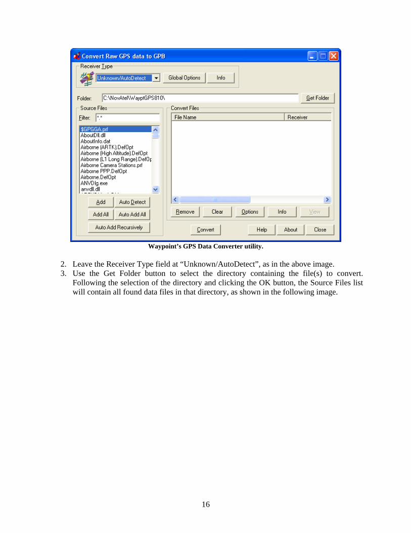
16

Waypoint’s GPS Data Converter utility.

2. Leave the Receiver Type field at “Unknown/AutoDetect”, as in the above image. 3. Use the Get Folder button to select the directory containing the file(s) to convert.

Following the selection of the directory and clicking the OK button, the Source Files list will contain all found data files in that directory, as shown in the following image.

17

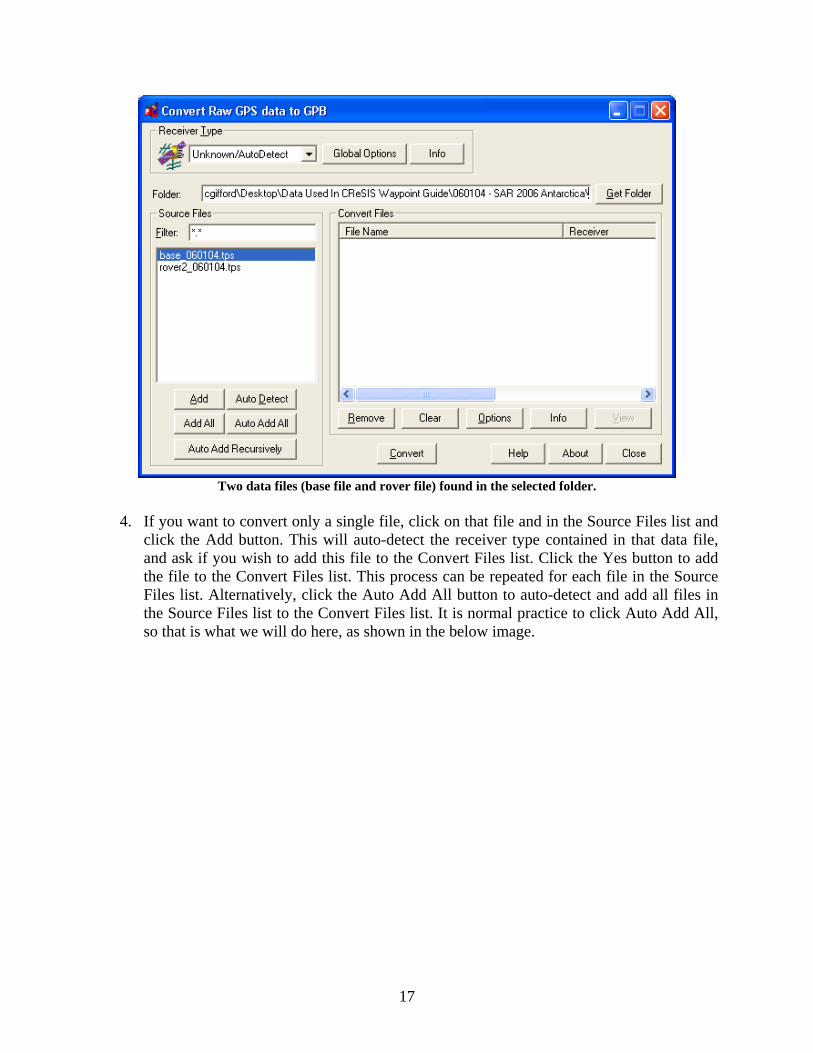
Two data files (base file and rover file) found in the selected folder.

4. If you want to convert only a single file, click on that file and in the Source Files list and

click the Add button. This will auto-detect the receiver type contained in that data file, and ask if you wish to add this file to the Convert Files list. Click the Yes button to add the file to the Convert Files list. This process can be repeated for each file in the Source Files list. Alternatively, click the Auto Add All button to auto-detect and add all files in the Source Files list to the Convert Files list. It is normal practice to click Auto Add All, so that is what we will do here, as shown in the below image.

18

Adding all files in the selected directory to the Convert Files list, all of which have their data auto-detected.

5. If there is a need to adjust how each individual file will be converted (based on detected

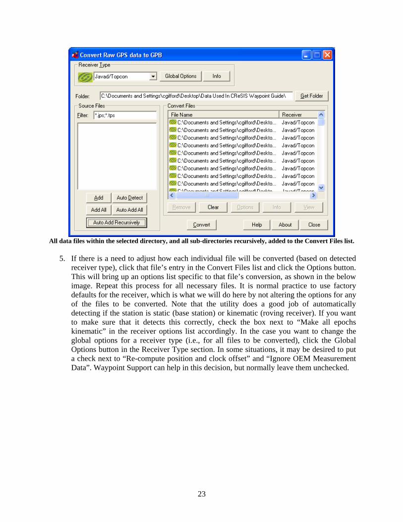
receiver type), click that file’s entry in the Convert Files list and click the Options button. This will bring up an options list specific to that file’s conversion, as shown in the below image. Repeat this process for all necessary files. It is normal practice to use factory defaults for the receiver, which is what we will do here by not altering the options for any of the files to be converted. Note that the utility does a good job of automatically detecting if the station is static (base station) or kinematic (roving receiver). If you want to make sure that it detects this correctly, check the box next to “Make all epochs kinematic” in the receiver options list accordingly.

19

File conversion options for a Javad/Topcon receiver. This image shows the factory defaults for Javad/Topcon.

6. Once all data files to convert have been added to the Convert Files list and their options set, click the Convert button to begin the conversion process of those files.

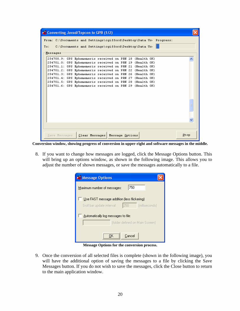
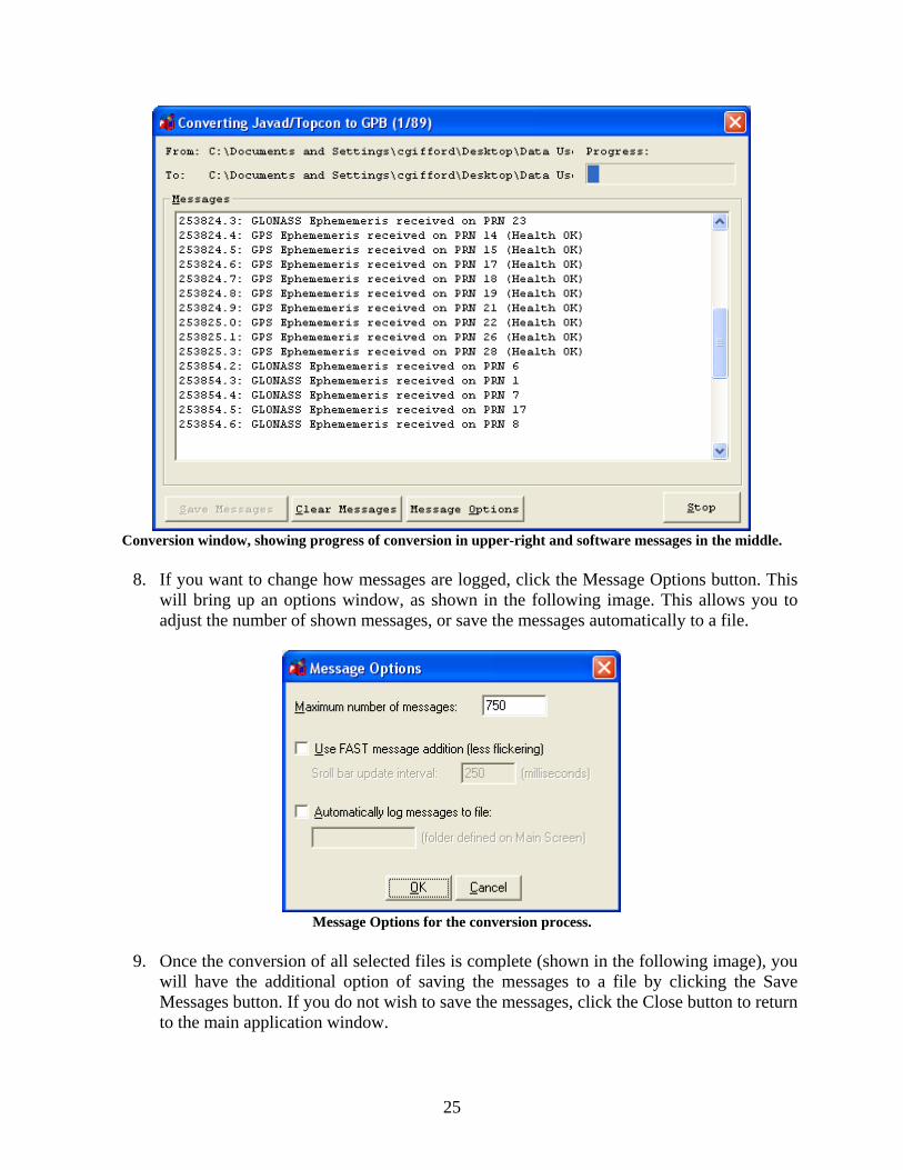
7. A conversion window will appear, showing messages from the software about the data. This is shown in the following image. By default, once 750 messages have been output, no more will be shown. Click the Clear Messages button to clear the message list if you see a message stating “Maximum 750 message received. Press Clear Messages to see more”. Even if this message is shown, the conversion process continues.

20

Conversion window, showing progress of conversion in upper-right and software messages in the middle.

8. If you want to change how messages are logged, click the Message Options button. This

will bring up an options window, as shown in the following image. This allows you to adjust the number of shown messages, or save the messages automatically to a file.

Message Options for the conversion process.

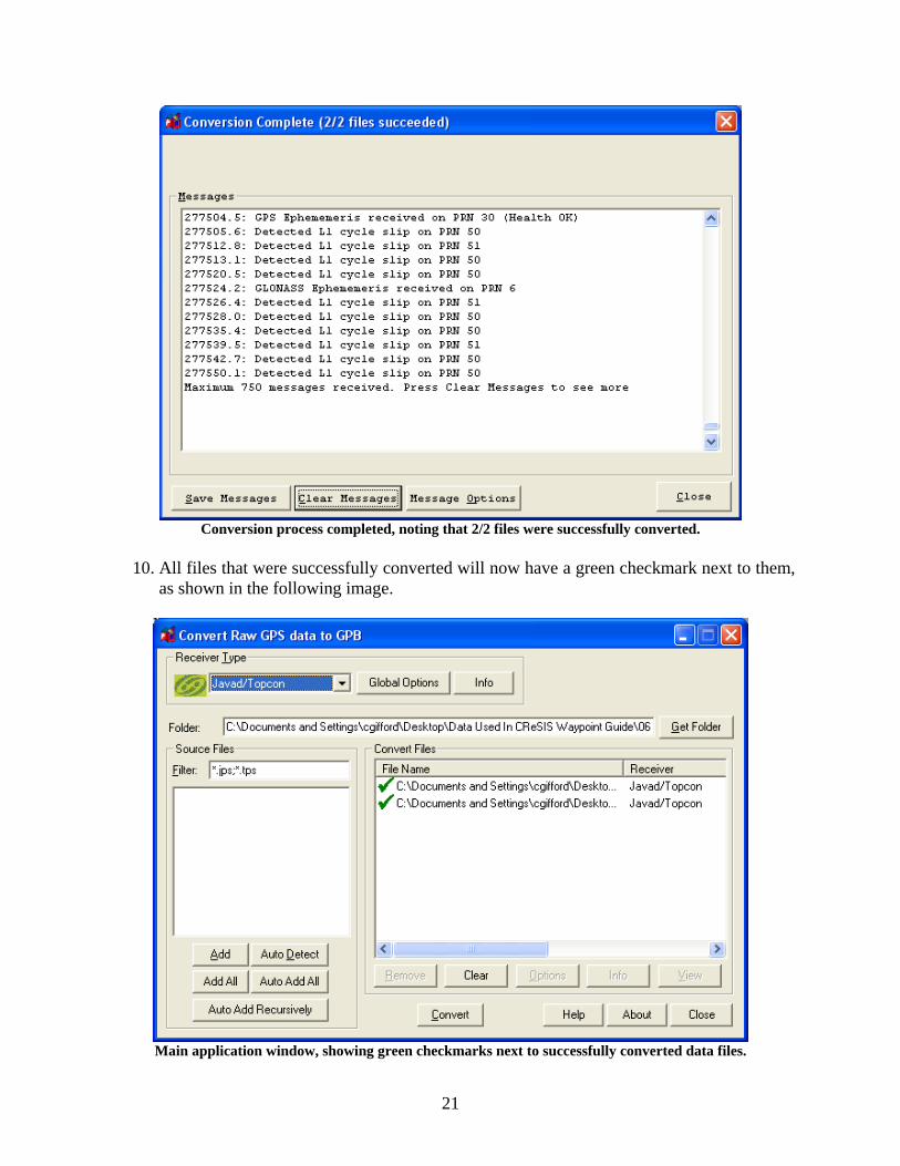
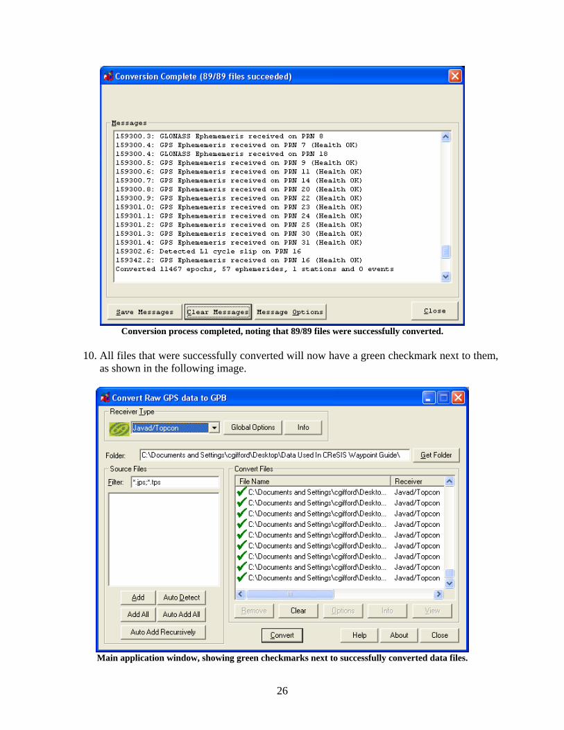
9. Once the conversion of all selected files is complete (shown in the following image), you

will have the additional option of saving the messages to a file by clicking the Save Messages button. If you do not wish to save the messages, click the Close button to return to the main application window.

21

Conversion process completed, noting that 2/2 files were successfully converted.

10. All files that were successfully converted will now have a green checkmark next to them,

as shown in the following image.

Main application window, showing green checkmarks next to successfully converted data files.

22

11. Check the station (.sta) files produced by the converter to ensure the conversion process went well. This file contains information specific to each converted file, such as whether the data is static (base station) or kinematic (roving receiver), the antenna height used during the recording process, and the type of antenna. If any of this information is wrong, convert the data again using different receiver options for those files. The below examples illustrate this.

Base station STA file:

Mark File: 253823.8 ENTERING STATIC MODE STA: * 253823.77 * base * 3.500 * * JPSLEGANT_E *

Roving receiver STA file: Mark File: 253095.8 ENTERING KINEMATIC MODE STA: * 253095.76 * rover2 * 2.000 * * JPSLEGANT_E * 277502.9 ENTERING KINEMATIC MODE STA: * 277502.90 * rover2 * 2.000 * * JPSLEGANT_E *

12. If the conversion process went well, you now have the option of deleting the original data

files you converted from. For large files this may save space, but may be desired for redundancy purposes. The above process can be repeated to convert other directories of data files. See the other Waypoint support materials for more information.

Example 2: Convert all Topcon TPS data files in a directory and all of its sub-directories

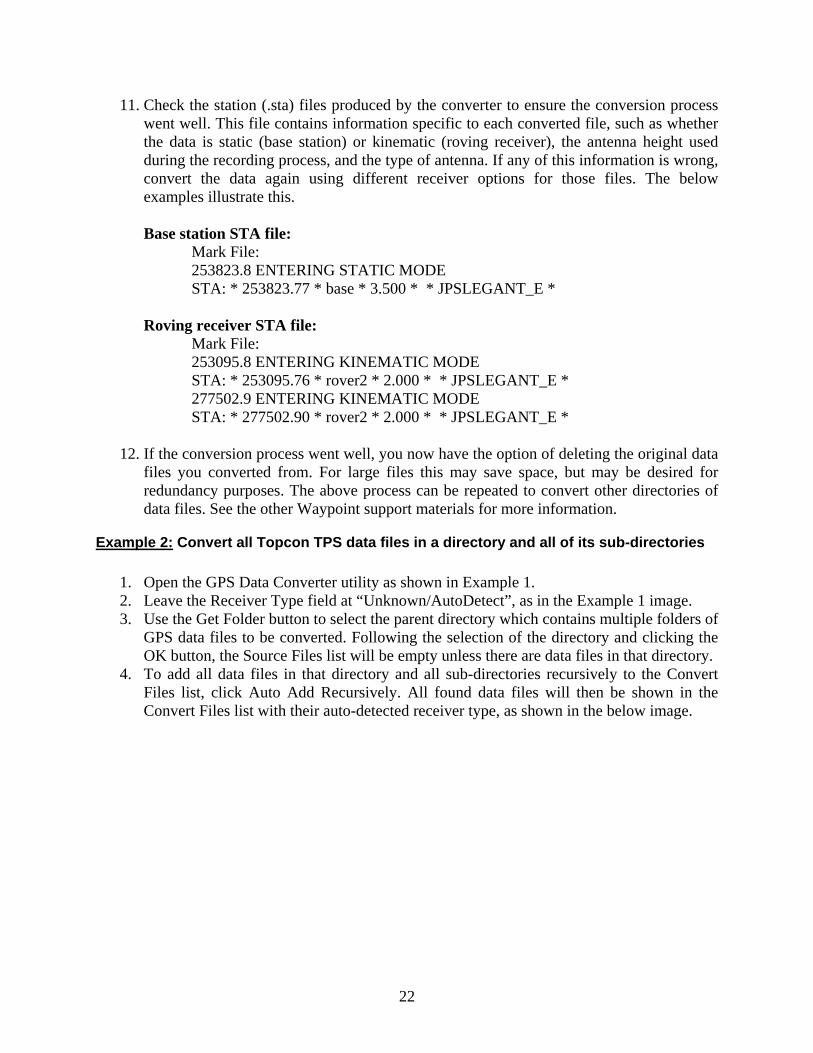
1. Open the GPS Data Converter utility as shown in Example 1. 2. Leave the Receiver Type field at “Unknown/AutoDetect”, as in the Example 1 image. 3. Use the Get Folder button to select the parent directory which contains multiple folders of

GPS data files to be converted. Following the selection of the directory and clicking the OK button, the Source Files list will be empty unless there are data files in that directory.

4. To add all data files in that directory and all sub-directories recursively to the Convert Files list, click Auto Add Recursively. All found data files will then be shown in the Convert Files list with their auto-detected receiver type, as shown in the below image.

23

All data files within the selected directory, and all sub-directories recursively, added to the Convert Files list.

5. If there is a need to adjust how each individual file will be converted (based on detected receiver type), click that file’s entry in the Convert Files list and click the Options button. This will bring up an options list specific to that file’s conversion, as shown in the below image. Repeat this process for all necessary files. It is normal practice to use factory defaults for the receiver, which is what we will do here by not altering the options for any of the files to be converted. Note that the utility does a good job of automatically detecting if the station is static (base station) or kinematic (roving receiver). If you want to make sure that it detects this correctly, check the box next to “Make all epochs kinematic” in the receiver options list accordingly. In the case you want to change the global options for a receiver type (i.e., for all files to be converted), click the Global Options button in the Receiver Type section. In some situations, it may be desired to put a check next to “Re-compute position and clock offset” and “Ignore OEM Measurement Data”. Waypoint Support can help in this decision, but normally leave them unchecked.

24

File conversion options for a Javad/Topcon receiver. This image shows the factory defaults for Javad/Topcon.

6. Once all data files to convert have been added to the Convert Files list and their options set, click the Convert button to begin the conversion process of those files.

7. A conversion window will appear, showing messages from the software about the data. This is shown in the following image. By default, once 750 messages have been output, no more will be shown. Click the Clear Messages button to clear the message list if you see a message stating “Maximum 750 message received. Press Clear Messages to see more”. Even if this message is shown, the conversion process continues.

25

Conversion window, showing progress of conversion in upper-right and software messages in the middle.

8. If you want to change how messages are logged, click the Message Options button. This

will bring up an options window, as shown in the following image. This allows you to adjust the number of shown messages, or save the messages automatically to a file.

Message Options for the conversion process.

9. Once the conversion of all selected files is complete (shown in the following image), you

will have the additional option of saving the messages to a file by clicking the Save Messages button. If you do not wish to save the messages, click the Close button to return to the main application window.

26

Conversion process completed, noting that 89/89 files were successfully converted.

10. All files that were successfully converted will now have a green checkmark next to them,

as shown in the following image.

Main application window, showing green checkmarks next to successfully converted data files.

27

11. Check the station (.sta) files produced by the converter to ensure the conversion process went well, as shown in Example 1.

12. If the conversion process went well, you now have the option of deleting the original data files you converted from. For large files this may save space, but may be desired for redundancy purposes. The above process can be repeated to convert other directories containing nested directories of data files. See the other Waypoint support materials for more information.

Concatenate, Slice, and Resample Data Waypoint Utility Occasionally there is the need to break files up into chunks, make multiple files into one, or resample the data we gather. This utility provides these functions for collections of one or more raw data files in GPB format. The result of these operations is also in GPB format. A typical use of this software is to resample a data file from high update rates to having much fewer updates for faster processing. We will mostly use it for this purpose, as well as concatenating past data from several files each with 30 minutes of data to a single file containing a day of data. The following steps can be used for general data and file manipulation. The below examples are for Topcon data, as it has been used extensively and is currently being used in the field. Note that files cannot be combined if they are not in sequential order or if they overlap in time. This utility also supports operations not shown in these examples. For details on these, see the other Waypoint support documents for more information.

Example 1: Combine multiple base station data files, each containing 30 minutes of data

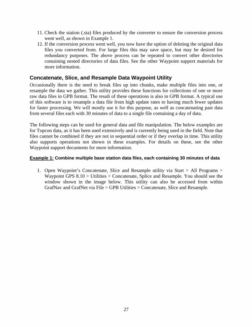
1. Open Waypoint’s Concatenate, Slice and Resample utility via Start > All Programs > Waypoint GPS 8.10 > Utilities > Concatenate, Splice and Resample. You should see the window shown in the image below. This utility can also be accessed from within GrafNav and GrafNet via File > GPB Utilities > Concatenate, Slice and Resample.

28

Waypoint’s Concatenate, Splice and Resample utility.

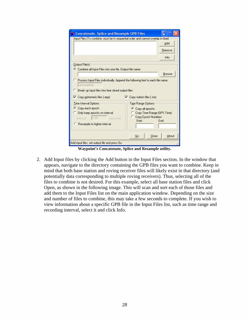
2. Add Input files by clicking the Add button in the Input Files section. In the window that

appears, navigate to the directory containing the GPB files you want to combine. Keep in mind that both base station and roving receiver files will likely exist in that directory (and potentially data corresponding to multiple roving receivers). Thus, selecting all of the files to combine is not desired. For this example, select all base station files and click Open, as shown in the following image. This will scan and sort each of those files and add them to the Input Files list on the main application window. Depending on the size and number of files to combine, this may take a few seconds to complete. If you wish to view information about a specific GPB file in the Input Files list, such as time range and recording interval, select it and click Info.

29

Selecting the base station input files for combining. Note that there are two sets of rover files (1 and 2).

Viewing information about a GPB file via the Info button in the Concatenate, Splice and Resample utility.

3. Under the Output File(s) section, select to “Combine all Input Files into one file”. Click

the Browse button to select the output directory, fill in the “File name” field, and click Save.

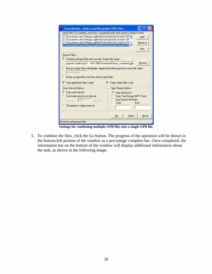
4. Ensure your window looks exactly like the following image for options, where we want to copy ephemeris files, station files, Copy each epoch, and Copy all epochs.

30

Settings for combining multiple GPB files into a single GPB file.

5. To combine the files, click the Go button. The progress of the operation will be shown in

the bottom-left portion of the window as a percentage complete bar. Once completed, the information bar on the bottom of the window will display additional information about the task, as shown in the following image.

31

Completed combination of multiple GPB files, showing 212.86 out of 212.86 MB of data was combined.

6. This process will produce three total files: base_combined.gpb, base_combined.epp, and

base_combined.sta. As before, the station file can be checked for validity. These files can now be used for post-processing. If doing a kinematic survey, repeat this process for accompanying roving receiver files.

7. The original GPB data files that have now been combined can be safely deleted, as this same utility can be used to splice the data back into 30 minute chunks (Example 2). See the other Waypoint support materials for more information.

Example 2: Splice a base station data file into multiple files, each with 30 minutes of data

1. Open the Concatenate, Splice and Resample utility as shown in Example 1. 2. Add Input files by clicking the Add button in the Input Files section. In the window that

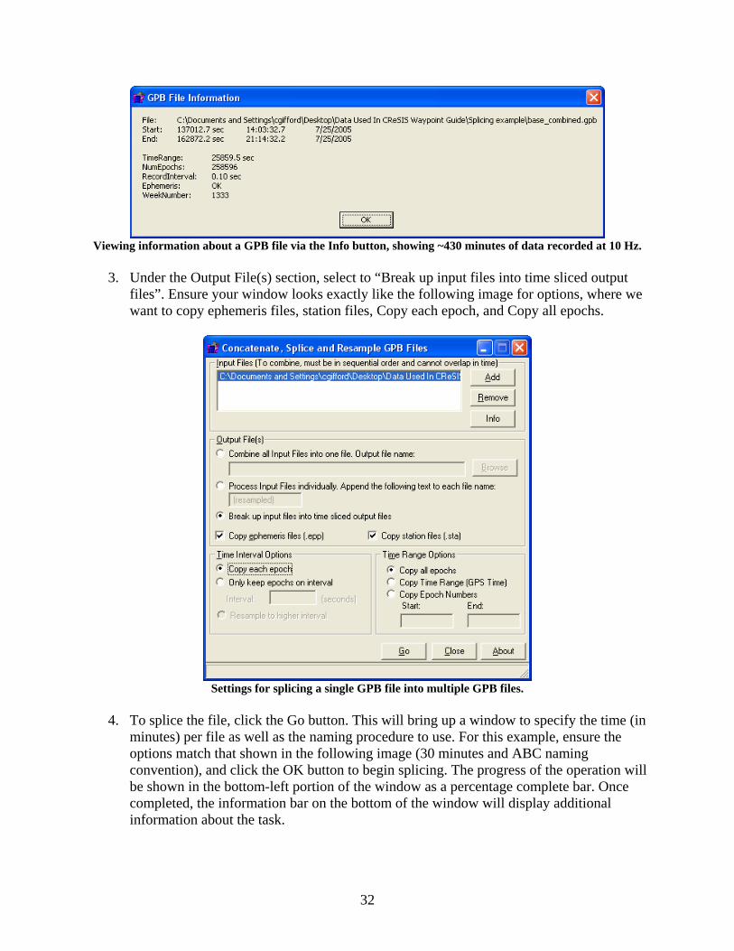
appears, navigate to the directory containing the GPB file(s) you want to splice. For this example, select the base station file and click Open. Multiple files can be selected to individually splice using the same options. This will scan that file and add it to the Input Files list on the main application window. Depending on the size and number of files to combine, this may take a few seconds to complete. If you wish to view information about a specific GPB file in the Input Files list, such as time range and recording interval, select it and click Info, as shown in the following image.

32

Viewing information about a GPB file via the Info button, showing ~430 minutes of data recorded at 10 Hz.

3. Under the Output File(s) section, select to “Break up input files into time sliced output

files”. Ensure your window looks exactly like the following image for options, where we want to copy ephemeris files, station files, Copy each epoch, and Copy all epochs.

Settings for splicing a single GPB file into multiple GPB files.

4. To splice the file, click the Go button. This will bring up a window to specify the time (in

minutes) per file as well as the naming procedure to use. For this example, ensure the options match that shown in the following image (30 minutes and ABC naming convention), and click the OK button to begin splicing. The progress of the operation will be shown in the bottom-left portion of the window as a percentage complete bar. Once completed, the information bar on the bottom of the window will display additional information about the task.

33

Options for splicing a GPB file up into 30 minute chunks.

Completed splicing of GPB file into multiple files, showing a total of fifteen 30-minute files being produced.

5. This process will produce three files for each splice: *.gpb, *.epp, and *.sta. As before,

the station file for each can be checked for validity. These files can now be used for post-processing. If doing a kinematic survey, repeat this process for accompanying roving receiver files.

6. The original GPB data file that has now been spliced can be safely deleted, as this same utility can be used to combine the data back into a single file (Example 1). See the other Waypoint support materials for more information.

Example 3: Resample a base station file to only keep data at 30 second intervals

1. Open the Concatenate, Splice and Resample utility as shown in Example 1.

34

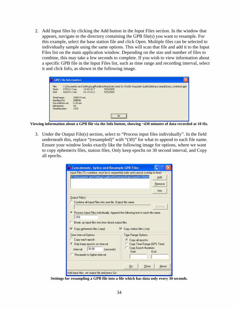
2. Add Input files by clicking the Add button in the Input Files section. In the window that appears, navigate to the directory containing the GPB file(s) you want to resample. For this example, select the base station file and click Open. Multiple files can be selected to individually sample using the same options. This will scan that file and add it to the Input Files list on the main application window. Depending on the size and number of files to combine, this may take a few seconds to complete. If you wish to view information about a specific GPB file in the Input Files list, such as time range and recording interval, select it and click Info, as shown in the following image.

Viewing information about a GPB file via the Info button, showing ~430 minutes of data recorded at 10 Hz.

3. Under the Output File(s) section, select to “Process input files individually”. In the field

underneath this, replace “(resampled)” with “(30)” for what to append to each file name. Ensure your window looks exactly like the following image for options, where we want to copy ephemeris files, station files, Only keep epochs on 30 second interval, and Copy all epochs.

Settings for resampling a GPB file into a file which has data only every 30 seconds.

35

4. To resample the file, click the Go button. The progress of the operation will be shown in the bottom-left portion of the window as a percentage complete bar. Once completed, the information bar on the bottom of the window will display additional information about the task.

Completed the resampling of a GPB file, showing that it copied 0.55 out of 165.18 MB (30 second interval).

5. This process will produce three files for each splice: “* (30).gpb”, “* (30).epp”, and “*

(30).sta”. As before, the station file for each can be checked for validity. Also, you can re-add the file that was created (with “(30)” appended) and click Info. A 30.00 second recording interval should be listed, as illustrated in the following image.

Checking the resampled result using the Info button, showing the desired 30.00 second recording interval.

6. These files can now be used for post-processing. If doing a kinematic survey, repeat this

process for accompanying roving receiver files. See the other Waypoint support materials for more information.

36

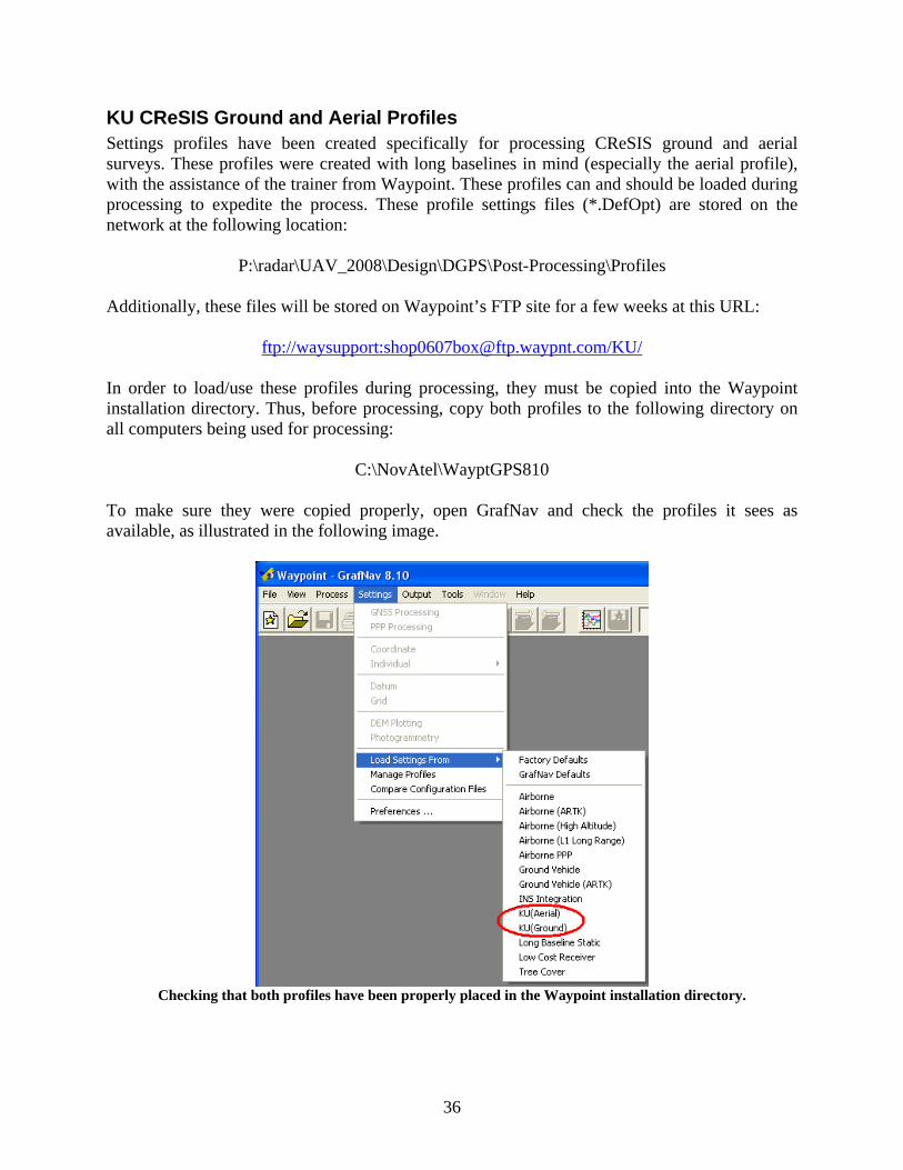
KU CReSIS Ground and Aerial Profiles Settings profiles have been created specifically for processing CReSIS ground and aerial surveys. These profiles were created with long baselines in mind (especially the aerial profile), with the assistance of the trainer from Waypoint. These profiles can and should be loaded during processing to expedite the process. These profile settings files (*.DefOpt) are stored on the network at the following location:

P:\radar\UAV_2008\Design\DGPS\Post-Processing\Profiles Additionally, these files will be stored on Waypoint’s FTP site for a few weeks at this URL:

ftp://waysupport:shop0607box@ftp.waypnt.com/KU/ In order to load/use these profiles during processing, they must be copied into the Waypoint installation directory. Thus, before processing, copy both profiles to the following directory on all computers being used for processing:

C:\NovAtel\WayptGPS810 To make sure they were copied properly, open GrafNav and check the profiles it sees as available, as illustrated in the following image.

Checking that both profiles have been properly placed in the Waypoint installation directory.

37

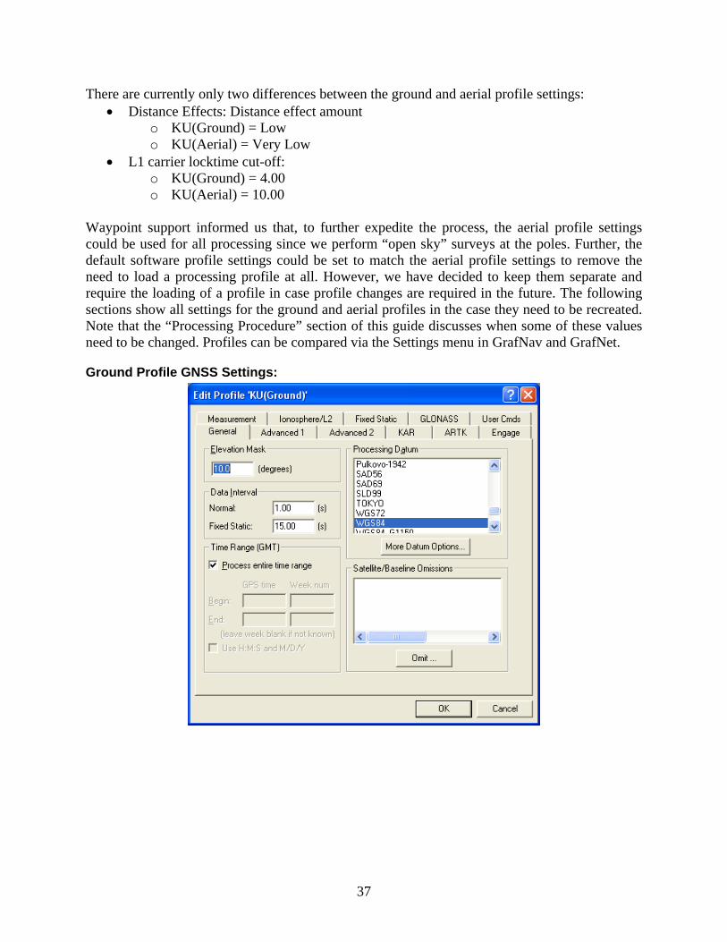
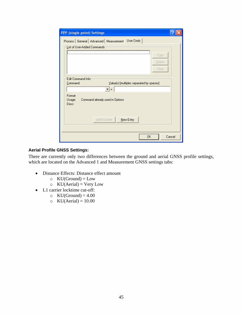
There are currently only two differences between the ground and aerial profile settings: • Distance Effects: Distance effect amount

o KU(Ground) = Low o KU(Aerial) = Very Low

• L1 carrier locktime cut-off: o KU(Ground) = 4.00 o KU(Aerial) = 10.00

Waypoint support informed us that, to further expedite the process, the aerial profile settings could be used for all processing since we perform “open sky” surveys at the poles. Further, the default software profile settings could be set to match the aerial profile settings to remove the need to load a processing profile at all. However, we have decided to keep them separate and require the loading of a profile in case profile changes are required in the future. The following sections show all settings for the ground and aerial profiles in the case they need to be recreated. Note that the “Processing Procedure” section of this guide discusses when some of these values need to be changed. Profiles can be compared via the Settings menu in GrafNav and GrafNet.

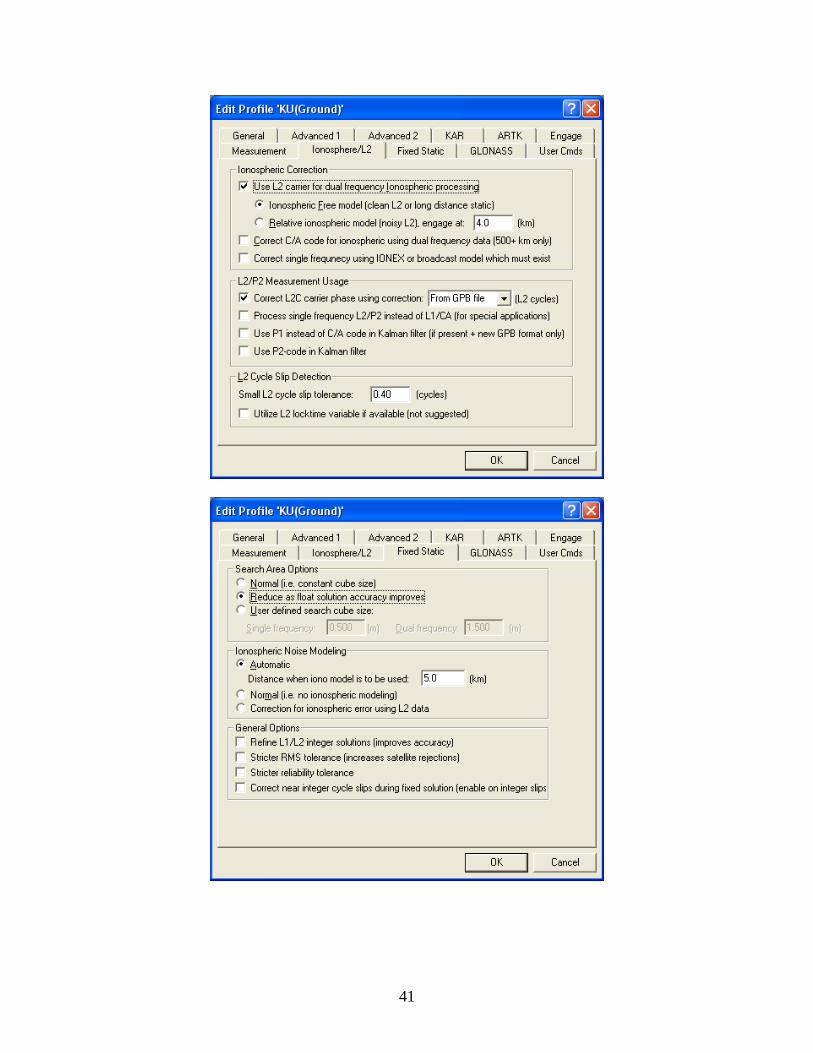
Ground Profile GNSS Settings:

38

39

40

41

42

43

Ground Profile PPP Settings:

44

45

Aerial Profile GNSS Settings: There are currently only two differences between the ground and aerial GNSS profile settings, which are located on the Advanced 1 and Measurement GNSS settings tabs:

• Distance Effects: Distance effect amount o KU(Ground) = Low o KU(Aerial) = Very Low

• L1 carrier locktime cut-off: o KU(Ground) = 4.00 o KU(Aerial) = 10.00

46

Aerial Profile PPP Settings: There is only one difference between the ground and aerial PPP profile settings, which is on the Advanced tab of the PPP settings:

47

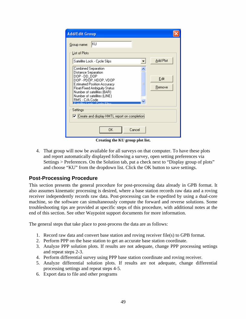
KU Group Plots There are several plots available to view after processing a survey, but only some of them are important to us. We can expedite the process of viewing and analyzing plots by automatically displaying the list of plots we specifically want to view after post-processing. To do this, we need to create a plot group, which we will call “KU”. The following steps go over creating this plot group:

1. Open GrafNav via Start > All Programs > Waypoint GPS 8.10 > GrafNav. GrafNav will open and try to find the hardlock key.

2. Open the plot settings window via Output > Plot Results. The following window will appear. If you do not see “KU” under Plots > Grouped Plots in that window, the group needs to be created. Click the Add Group button to create your own group of plots.

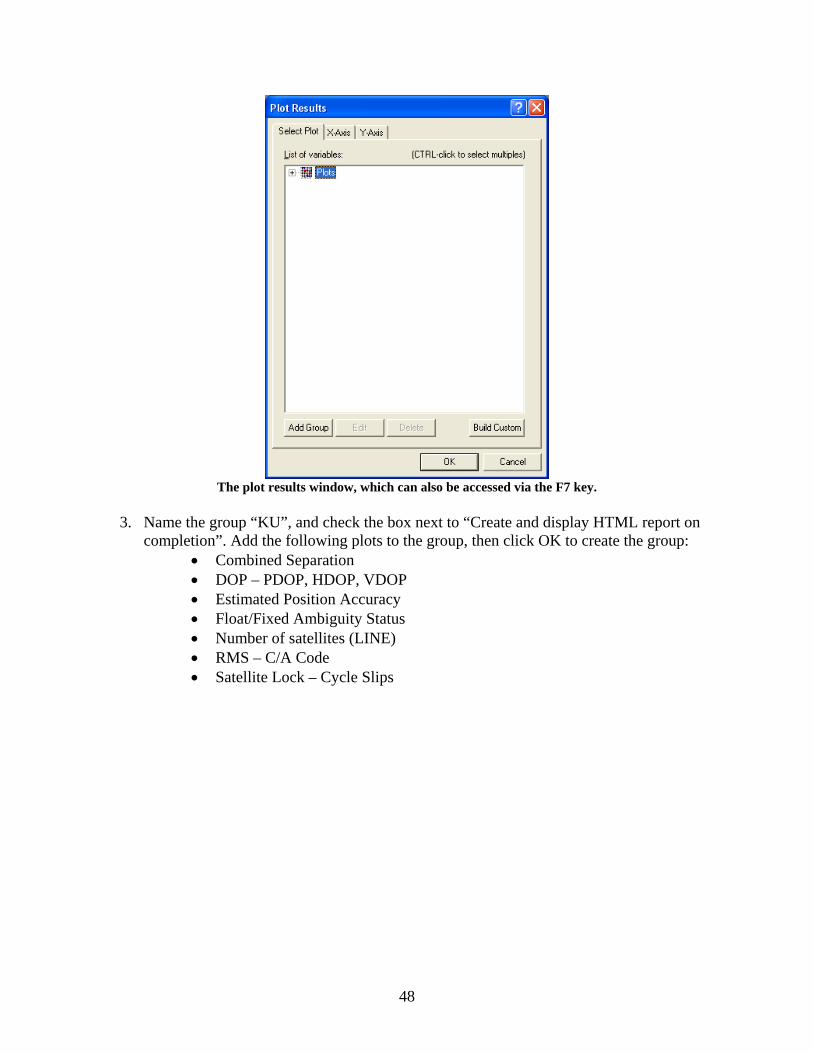
48

The plot results window, which can also be accessed via the F7 key.

3. Name the group “KU”, and check the box next to “Create and display HTML report on

completion”. Add the following plots to the group, then click OK to create the group: • Combined Separation • DOP – PDOP, HDOP, VDOP • Estimated Position Accuracy • Float/Fixed Ambiguity Status • Number of satellites (LINE) • RMS – C/A Code • Satellite Lock – Cycle Slips

49

Creating the KU group plot list.

4. That group will now be available for all surveys on that computer. To have these plots

and report automatically displayed following a survey, open setting preferences via Settings > Preferences. On the Solution tab, put a check next to “Display group of plots” and choose “KU” from the dropdown list. Click the OK button to save settings.

Post-Processing Procedure This section presents the general procedure for post-processing data already in GPB format. It also assumes kinematic processing is desired, where a base station records raw data and a roving receiver independently records raw data. Post-processing can be expedited by using a dual-core machine, so the software can simultaneously compute the forward and reverse solutions. Some troubleshooting tips are provided at specific steps of this procedure, with additional notes at the end of this section. See other Waypoint support documents for more information. The general steps that take place to post-process the data are as follows:

1. Record raw data and convert base station and roving receiver file(s) to GPB format. 2. Perform PPP on the base station to get an accurate base station coordinate. 3. Analyze PPP solution plots. If results are not adequate, change PPP processing settings

and repeat steps 2-3. 4. Perform differential survey using PPP base station coordinate and roving receiver. 5. Analyze differential solution plots. If results are not adequate, change differential

processing settings and repeat steps 4-5. 6. Export data to file and other programs

50

1. Record Raw Data and Convert to GPB Format This is covered in previous sections of this guide. See those sections for details on logging raw data and converting files to GPB format for use in post-processing.

2. Perform PPP on Base Station Data to get an Accurate Base Station Coordinate The base station must first be accurately set before we can properly perform differential processing for the roving receiver. A PPP (precise point positioning) survey on the base station will provide us an accurate coordinate to use for differential processing. This coordinate will be saved as a favorite for use in later steps. Note: It is highly recommended to make sure the latest manufacturing files are available. This can be automatically done by GrafNav and GrafNet through preference settings. Open preferences via Settings > Preferences, and ensure there is a check in the Auto-Update section in the Update tab. The following steps can be used for general PPP processing of a base station:

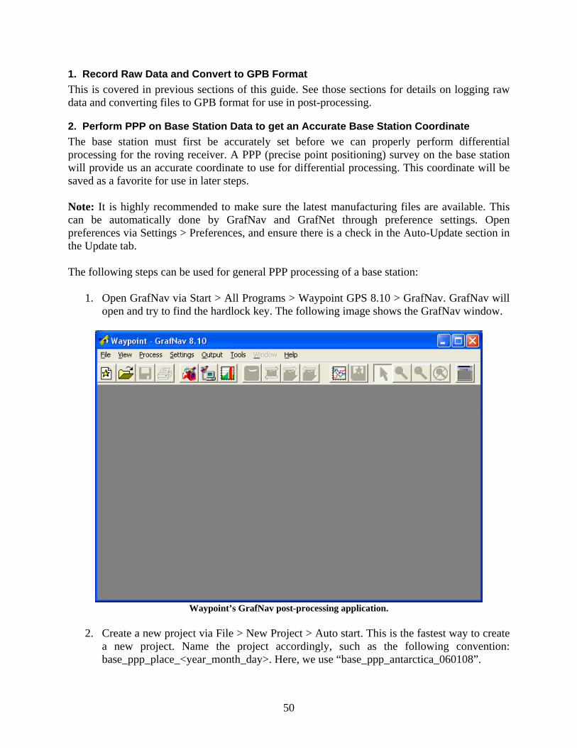
1. Open GrafNav via Start > All Programs > Waypoint GPS 8.10 > GrafNav. GrafNav will open and try to find the hardlock key. The following image shows the GrafNav window.

Waypoint’s GrafNav post-processing application.

2. Create a new project via File > New Project > Auto start. This is the fastest way to create

a new project. Name the project accordingly, such as the following convention: base_ppp_place_<year_month_day>. Here, we use “base_ppp_antarctica_060108”.

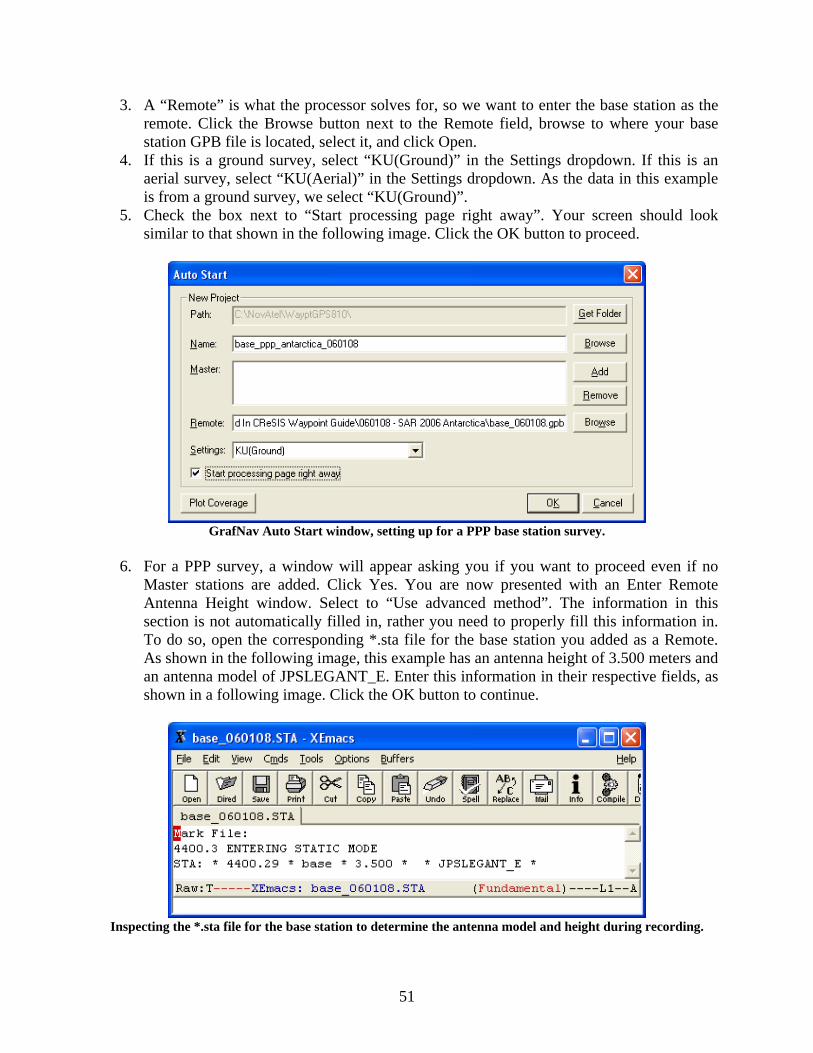
51

3. A “Remote” is what the processor solves for, so we want to enter the base station as the remote. Click the Browse button next to the Remote field, browse to where your base station GPB file is located, select it, and click Open.

4. If this is a ground survey, select “KU(Ground)” in the Settings dropdown. If this is an aerial survey, select “KU(Aerial)” in the Settings dropdown. As the data in this example is from a ground survey, we select “KU(Ground)”.

5. Check the box next to “Start processing page right away”. Your screen should look similar to that shown in the following image. Click the OK button to proceed.

GrafNav Auto Start window, setting up for a PPP base station survey.

6. For a PPP survey, a window will appear asking you if you want to proceed even if no

Master stations are added. Click Yes. You are now presented with an Enter Remote Antenna Height window. Select to “Use advanced method”. The information in this section is not automatically filled in, rather you need to properly fill this information in. To do so, open the corresponding *.sta file for the base station you added as a Remote. As shown in the following image, this example has an antenna height of 3.500 meters and an antenna model of JPSLEGANT_E. Enter this information in their respective fields, as shown in a following image. Click the OK button to continue.

Inspecting the *.sta file for the base station to determine the antenna model and height during recording.

52

Remote antenna information for the base station PPP survey.

7. You will again be warned that there are no master stations added. Click OK to proceed.

Close the two processing windows that automatically popped up, as they will not be needed. You will now be able to view your unprocessed base station data in the “Unprocessed – Map” window, along with its general accuracy before processing. The following image illustrates this for our example.

53

Viewing base station data in the Map window, ready to perform the PPP survey.

8. Click the “Process PPP Single Point” button on the middle of the toolbar. The following

window will appear. Note that the Status field states that there are no precise files present. These need to be downloaded by clicking on the Precise tab, and clicking the Download button. This will automatically download the correct precise clock and ephemeris files and add it to the project, as shown in a following image. Navigate back to the Process tab.

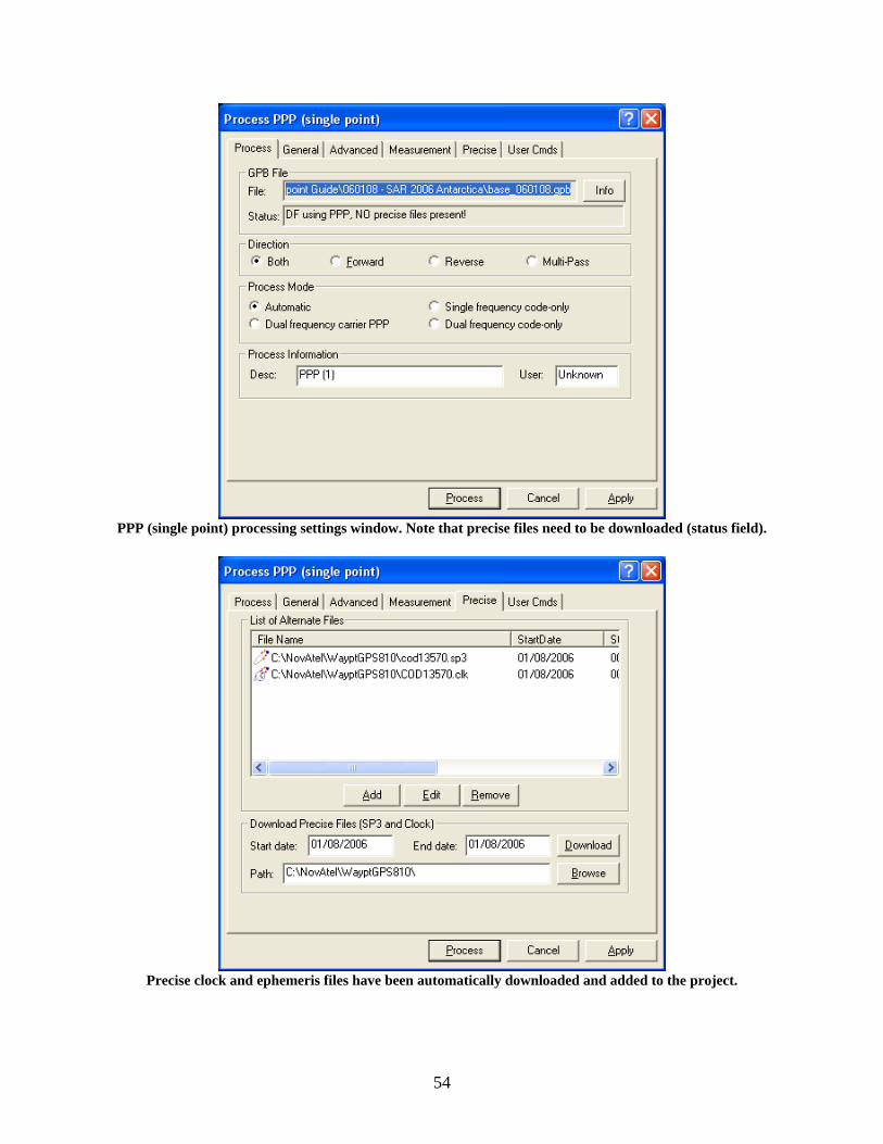
54

PPP (single point) processing settings window. Note that precise files need to be downloaded (status field).

Precise clock and ephemeris files have been automatically downloaded and added to the project.

55

9. Make sure Both is selected under the Direction section and Automatic is selected under the Process Mode section. Additional information can be provided in the Processing Information section, but is not required. Your screen should look like the following, with the Status field now saying we have precise clock and ephemeris files present. Navigate to the General tab.

Completed Process tab. Note that we now have precise clock and ephemeris files (status field).

10. As this is a base station and is static, we don’t necessarily need to use all of its 10 Hz

data. We could speed up processing time by replacing the 0.10 seconds in the Data Interval field to be 30.00 seconds. For this example, we leave the data at 10 Hz to get the best accuracy possible. All other tabs can be left as they are. Click the Process button to begin processing our PPP survey.

11. Solutions will now be computed in both forward and reverse directions. If using a dual-core CPU, both solutions will be computed simultaneously; otherwise, the forward will be computed and then the reverse sequentially. As shown in the following image, progress is shown in the upper-right area of the windows for each solution. The most important areas to look during this are in the Status section (top) and Notifications section (bottom). During processing, messages may appear that can give clues on how to resolve issues if results are not satisfactory. The status section provides a number which corresponds to the rank of the solution quality thus far, which should hopefully be 3 or lower. A fixed solution is desired, but will not always be attainable at our long baselines.

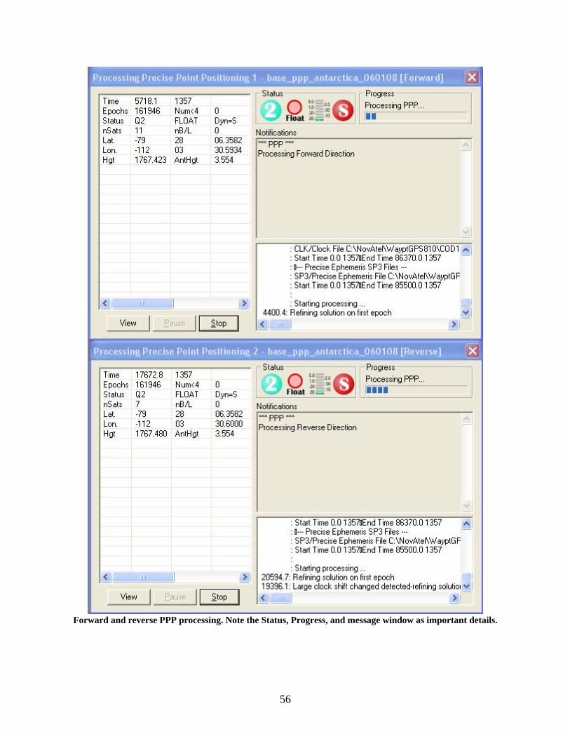
56

Forward and reverse PPP processing. Note the Status, Progress, and message window as important details.

57

After doing the PPP on the base station, we now have its coordinates down to under 2 cm error.

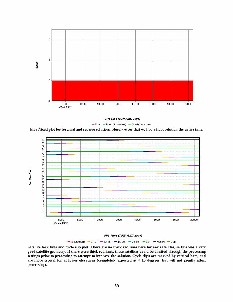
3. Analyze PPP Solution Plots Assuming the settings have been set to automatically display the KU group of plots, several plots should automatically appear and an HTML report should be automatically generated. The HTML report is a quick and easy way to view the results, but is not interactive. It can also be saved to file from your internet browser for future reference. The plot windows displayed by the software can be manipulated. For example, right-clicking and selecting to set the minimum and maximum facilitates zooming in and out. If large spikes are present in any of the images, this was likely due to a Kalman filter reset from bad satellite data or persistent cycle slips. The following images show the KU group plots for this PPP survey, with captions briefly discussing them.

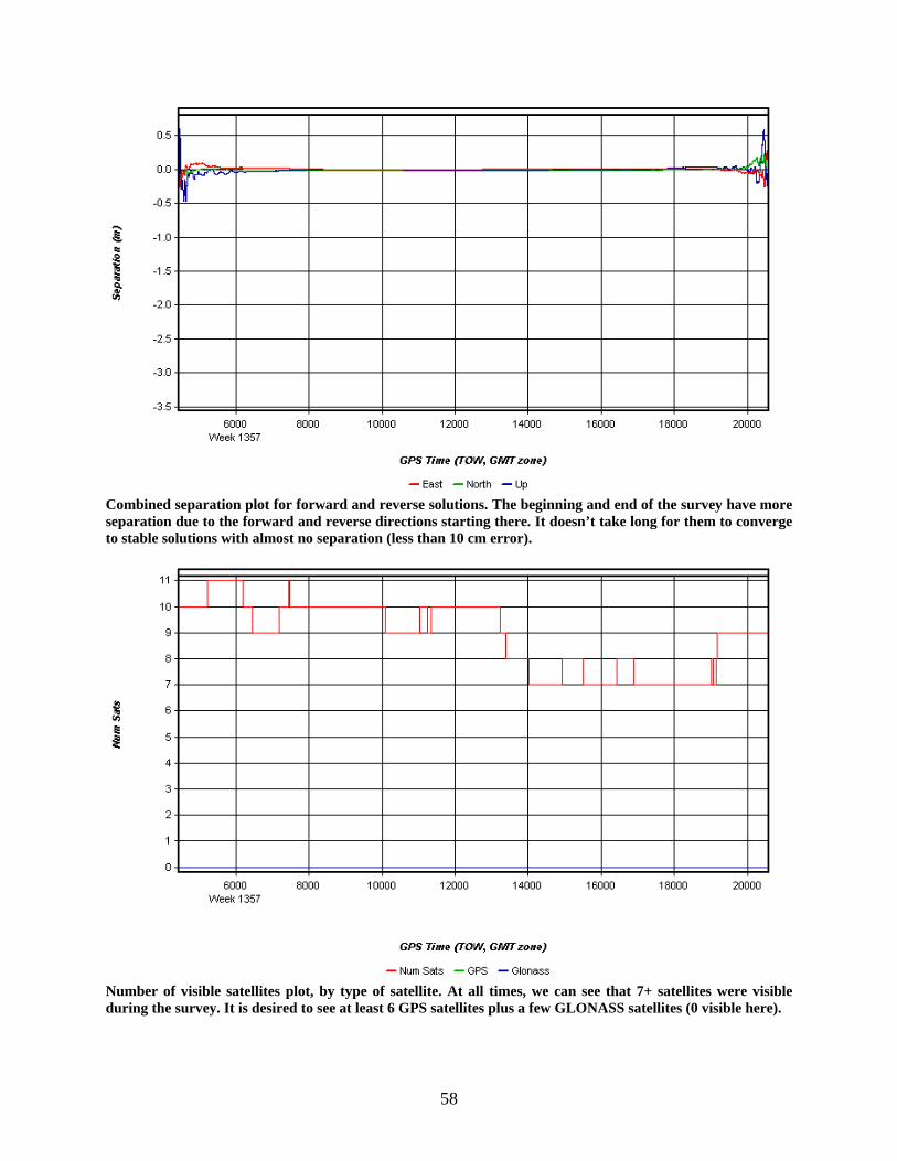
58

Combined separation plot for forward and reverse solutions. The beginning and end of the survey have more separation due to the forward and reverse directions starting there. It doesn’t take long for them to converge to stable solutions with almost no separation (less than 10 cm error).

Number of visible satellites plot, by type of satellite. At all times, we can see that 7+ satellites were visible during the survey. It is desired to see at least 6 GPS satellites plus a few GLONASS satellites (0 visible here).

59

Float/fixed plot for forward and reverse solutions. Here, we see that we had a float solution the entire time.

Satellite lock time and cycle slip plot. There are no thick red lines here for any satellites, so this was a very good satellite geometry. If there were thick red lines, those satellites could be omitted through the processing settings prior to processing to attempt to improve the solution. Cycle slips are marked by vertical bars, and are more typical for at lower elevations (completely expected at < 10 degrees, but will not greatly affect processing).

60

DOP plot, showing how horizontal (HDOP), vertical (VDOP), and XY (PDOP) accuracies were affected over the time of the survey. In regards to PDOP, it is generally accepted that values of 1-3 are considered excellent. Values of 3-4 are generally considered acceptable (although not ideal if you are trying to use KAR or ARTK), and 5-7 poor. Anything in the 8 or more is very poor. Again these are general guidelines. DDOP is roughly equal to PDOP^2. There are no drastic spikes in the plot, and all are under 4 for the DOP measures.

The RMS residuals plot. The red RMS line has no ramping, which is good. Ramps in RMS mean that the software was trying to fix satellite problems or the Kalman filter was reset. RMS is also always less than 7.

61

IMPORTANT: If results are satisfactory, save the processed base station coordinate to the Favorites via View > Objects > KAR/ARTK/Static. Click the Add to Favorites button, which will bring up the following window to adjust some information. Name the favorite “base_ppp_060108” and assign it to group KU. If the KU group is not there, click the Add Group button, enter “KU”, and click OK. Click OK to complete the addition of this base coordinate to favorites. This coordinate will be used when performing differential processing on the rover data.

Specifying information to save base station coordinate to Favorites for later use in differential processing.

4. Perform Differential Survey using PPP Base Station Coordinate and Roving Receiver Now that we have a processed PPP base station coordinate, we can proceed with the differential survey for the roving receiver. Again, using a dual-core CPU will increase the performance of processing. Note: For very long baselines (> 500 km), performing a PPP survey of the roving receiver has shown to be m much faster and sometimes provide better accuracy. The following steps can be performed for general post-processing of roving receiver data with a base station reference coordinate:

1. Open GrafNav as before via Start > All Programs > Waypoint GPS 8.10 > GrafNav. 2. Create a new project via File > New Project > Auto start. Name the project accordingly,

such as the following convention: rover_diff_place_<year_month_day>. Here, we use “rover_diff_antarctica_060108”.

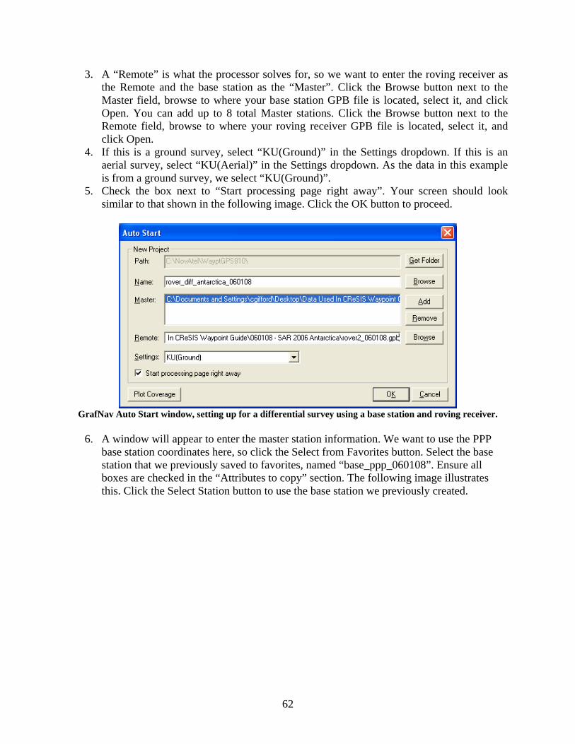
62

3. A “Remote” is what the processor solves for, so we want to enter the roving receiver as the Remote and the base station as the “Master”. Click the Browse button next to the Master field, browse to where your base station GPB file is located, select it, and click Open. You can add up to 8 total Master stations. Click the Browse button next to the Remote field, browse to where your roving receiver GPB file is located, select it, and click Open.

4. If this is a ground survey, select “KU(Ground)” in the Settings dropdown. If this is an aerial survey, select “KU(Aerial)” in the Settings dropdown. As the data in this example is from a ground survey, we select “KU(Ground)”.

5. Check the box next to “Start processing page right away”. Your screen should look similar to that shown in the following image. Click the OK button to proceed.

GrafNav Auto Start window, setting up for a differential survey using a base station and roving receiver.

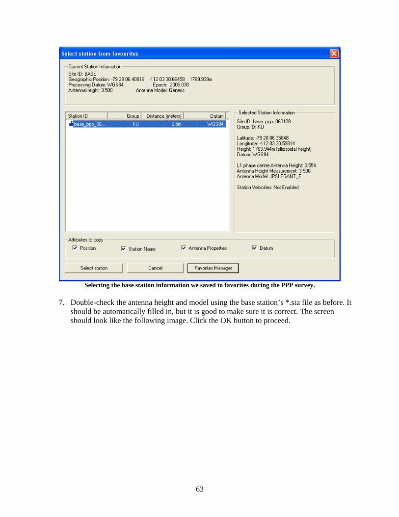
6. A window will appear to enter the master station information. We want to use the PPP

base station coordinates here, so click the Select from Favorites button. Select the base station that we previously saved to favorites, named “base_ppp_060108”. Ensure all boxes are checked in the “Attributes to copy” section. The following image illustrates this. Click the Select Station button to use the base station we previously created.

63

Selecting the base station information we saved to favorites during the PPP survey.

7. Double-check the antenna height and model using the base station’s *.sta file as before. It

should be automatically filled in, but it is good to make sure it is correct. The screen should look like the following image. Click the OK button to proceed.

64

Master base station coordinates retrieved from favorites and correct antenna information filled in.

8. You are now presented with an Enter Remote Antenna Height window. Select to “Use

advanced method”. The information in this section is not automatically filled in, rather you need to properly fill this information in. To do so, open the corresponding *.sta file for the roving receiver you added as a Remote. As shown in the following image, this example has an antenna height of 2.000 meters and an antenna model of JPSLEGANT_E. Enter this information in their respective fields, as shown in a following image. Click the OK button to continue.

Inspecting the *.sta file for the roving receiver to determine the antenna model and height during recording.

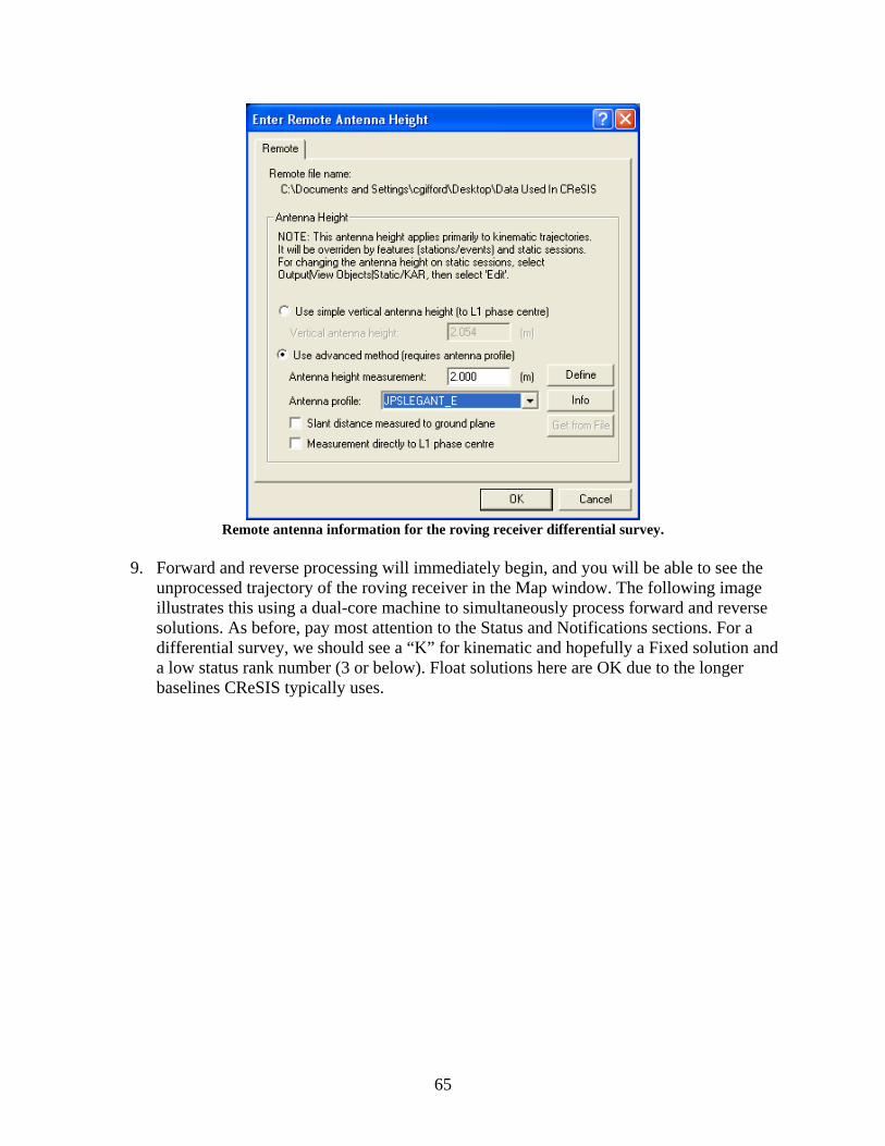
65

Remote antenna information for the roving receiver differential survey.

9. Forward and reverse processing will immediately begin, and you will be able to see the

unprocessed trajectory of the roving receiver in the Map window. The following image illustrates this using a dual-core machine to simultaneously process forward and reverse solutions. As before, pay most attention to the Status and Notifications sections. For a differential survey, we should see a “K” for kinematic and hopefully a Fixed solution and a low status rank number (3 or below). Float solutions here are OK due to the longer baselines CReSIS typically uses.

66

Processing forward and reverse solutions for a differential survey, with unprocessed trajectory shown (left).

5. Analyze Differential Solution Plots Now that we have processed the data, the result plots need to be analyzed to see if the solution is acceptable. Assuming the settings have been set to automatically display the KU group of plots, several plots should automatically appear and an HTML report should be automatically generated. The HTML report is a quick and easy way to view the results, but is not interactive. It can also be saved to file from your internet browser for future reference. The plot windows displayed by the software can be manipulated. For example, right-clicking and selecting to set the minimum and maximum facilitates zooming in and out. If large spikes are present in any of the images, this was likely due to a Kalman filter reset from bad satellite data or persistent cycle slips. The following images show the KU group plots for this differential survey, with captions briefly discussing them.

67

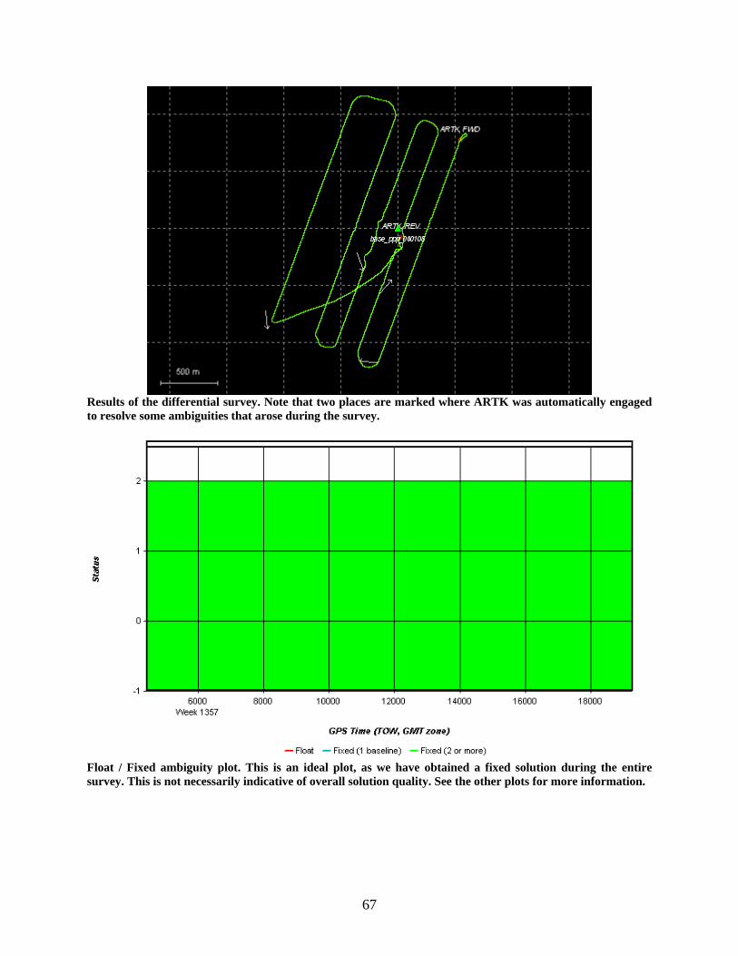
Results of the differential survey. Note that two places are marked where ARTK was automatically engaged to resolve some ambiguities that arose during the survey.

Float / Fixed ambiguity plot. This is an ideal plot, as we have obtained a fixed solution during the entire survey. This is not necessarily indicative of overall solution quality. See the other plots for more information.

68

Number of total visible satellites by constellation. Note that a maximum of 4 GLONASS satellites were visible at any one time during the survey. Total satellite coverage was sufficient for this survey (> 9 at all times).

Satellite lock / cycle slip plot. There are no thick red lines for any of the satellites, so we did not have any satellite troubles during this survey. If some satellites had thick red lines (very frequent cycle slips), we would want to omit those satellites (by number) in the processing settings. Also of note is that there were a few cycle slips (vertical red lines), but mostly at lower elevations (< 10 degrees). This is normal and expected, and generally will not greatly affect processing.

69

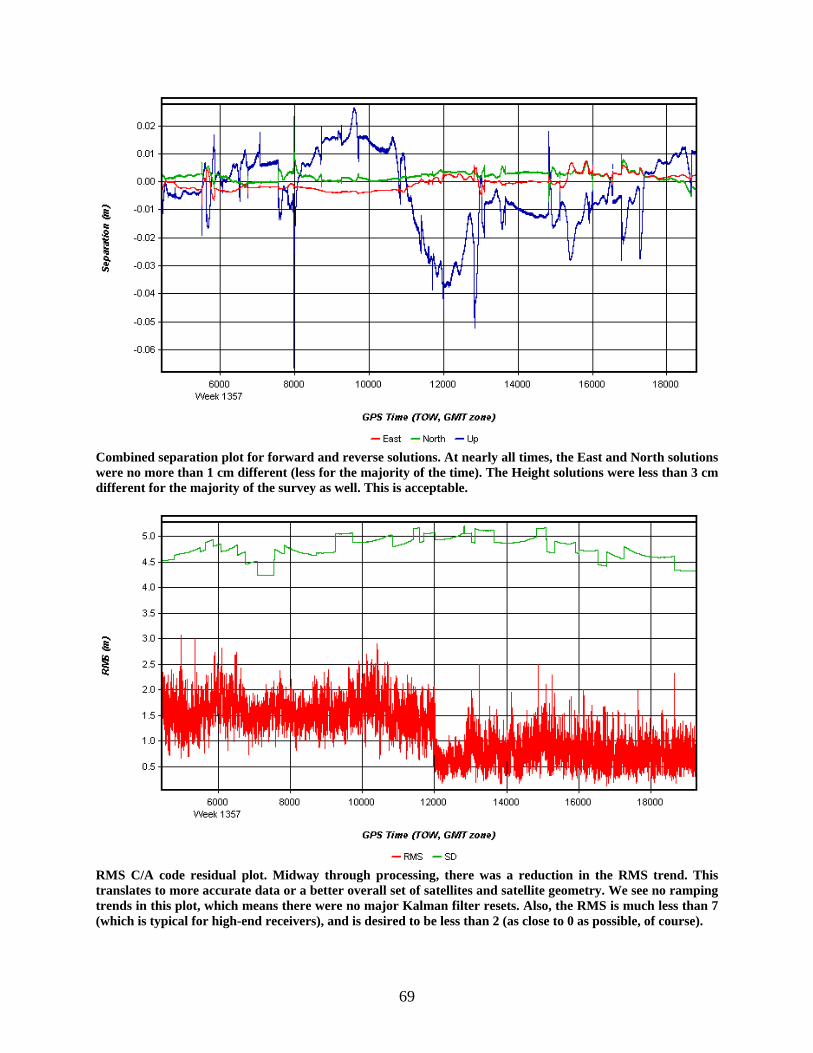
Combined separation plot for forward and reverse solutions. At nearly all times, the East and North solutions were no more than 1 cm different (less for the majority of the time). The Height solutions were less than 3 cm different for the majority of the survey as well. This is acceptable.

RMS C/A code residual plot. Midway through processing, there was a reduction in the RMS trend. This translates to more accurate data or a better overall set of satellites and satellite geometry. We see no ramping trends in this plot, which means there were no major Kalman filter resets. Also, the RMS is much less than 7 (which is typical for high-end receivers), and is desired to be less than 2 (as close to 0 as possible, of course).

70

DOP plot, showing the affects of horizontal (HDOP), vertical (VDOP), and XY (PDOP) accuracies. In regards to PDOP, it is generally accepted that values of 1-3 are considered excellent. Values of 3-4 are generally considered acceptable (although not ideal if you are trying to use KAR or ARTK), and 5-7 poor. Anything in the 8 or more is very poor. Again these are general guidelines. DDOP is roughly equal to PDOP^2. There are no major spikes present, and are all less than 3. This appears to be acceptable.

Estimated position accuracy plot. Note that the Trace line is the sum of the East, North, and Height lines. Height is always going to be less accurate than East and North, which we see here. The majority of the East and North data show standard deviation of 2 cm or better (one-sigma confidence). The Height data on the other hand mostly shows standard deviation of better than 8 cm (one-sigma confidence).

71

6. Export Data to File and Other Programs If plotted results are satisfactory, it is time to export the data of the final solution using the Export Coordinates Wizard. The following steps can be used to export the data in the proper CReSIS format. This is followed by an example of exporting the data to Google Earth for viewing.

Exporting Data to File in GPGGA Format The CReSIS radar data processing team uses GPS data in GPGGA format. The following steps can be used to export the processed data in this format:

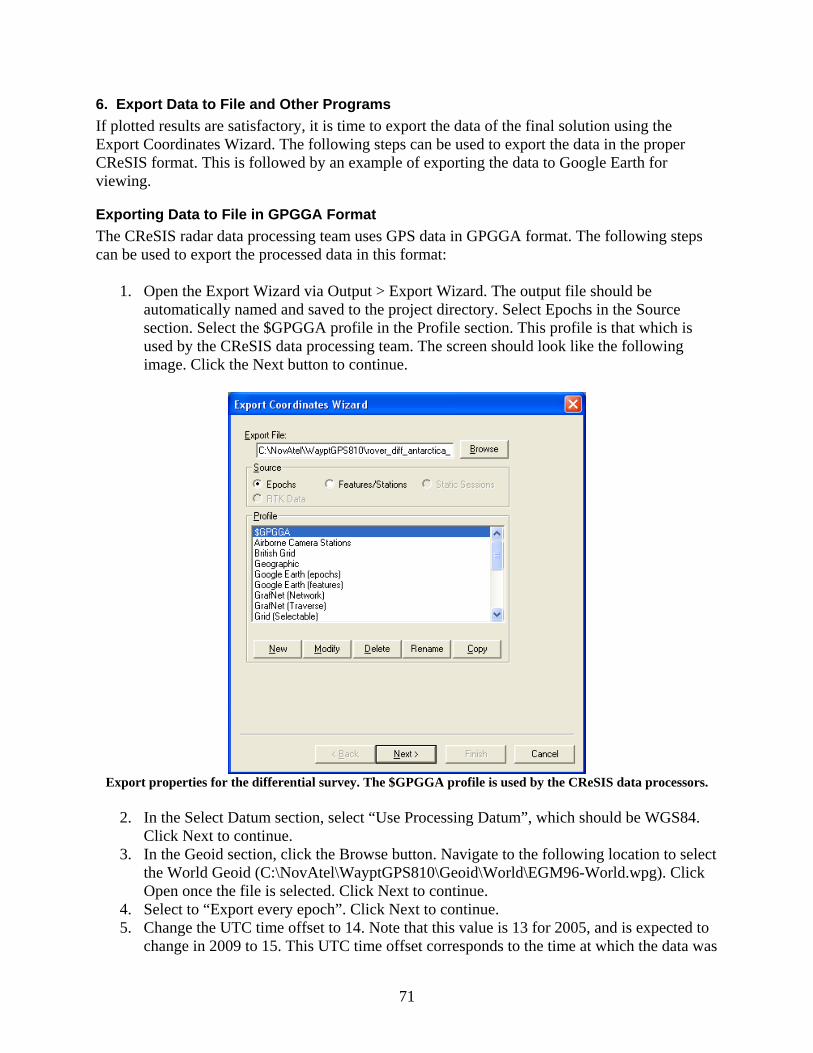
1. Open the Export Wizard via Output > Export Wizard. The output file should be automatically named and saved to the project directory. Select Epochs in the Source section. Select the $GPGGA profile in the Profile section. This profile is that which is used by the CReSIS data processing team. The screen should look like the following image. Click the Next button to continue.

Export properties for the differential survey. The $GPGGA profile is used by the CReSIS data processors.

2. In the Select Datum section, select “Use Processing Datum”, which should be WGS84.

Click Next to continue. 3. In the Geoid section, click the Browse button. Navigate to the following location to select

the World Geoid (C:\NovAtel\WayptGPS810\Geoid\World\EGM96-World.wpg). Click Open once the file is selected. Click Next to continue.

4. Select to “Export every epoch”. Click Next to continue. 5. Change the UTC time offset to 14. Note that this value is 13 for 2005, and is expected to

change in 2009 to 15. This UTC time offset corresponds to the time at which the data was

72

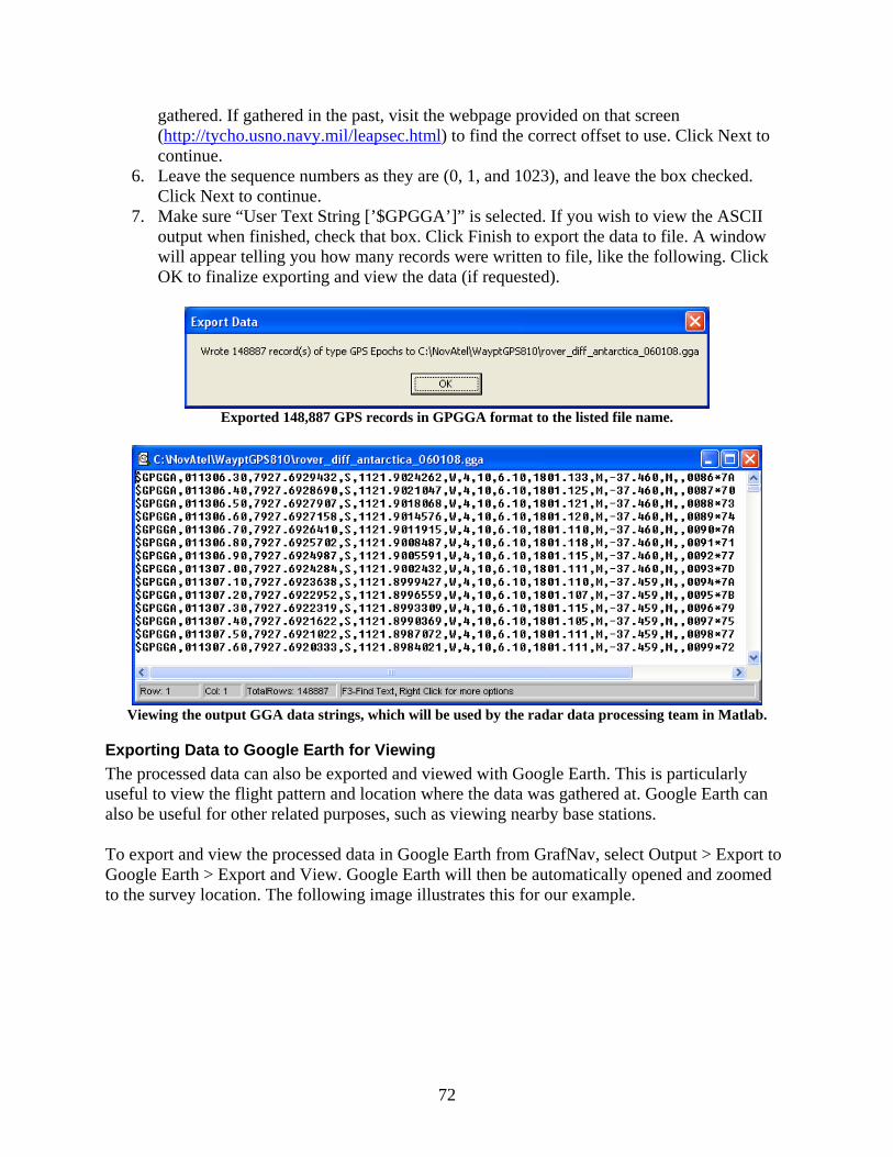
gathered. If gathered in the past, visit the webpage provided on that screen (http://tycho.usno.navy.mil/leapsec.html) to find the correct offset to use. Click Next to continue.

6. Leave the sequence numbers as they are (0, 1, and 1023), and leave the box checked. Click Next to continue.

7. Make sure “User Text String [’$GPGGA’]” is selected. If you wish to view the ASCII output when finished, check that box. Click Finish to export the data to file. A window will appear telling you how many records were written to file, like the following. Click OK to finalize exporting and view the data (if requested).

Exported 148,887 GPS records in GPGGA format to the listed file name.

Viewing the output GGA data strings, which will be used by the radar data processing team in Matlab.

Exporting Data to Google Earth for Viewing The processed data can also be exported and viewed with Google Earth. This is particularly useful to view the flight pattern and location where the data was gathered at. Google Earth can also be useful for other related purposes, such as viewing nearby base stations. To export and view the processed data in Google Earth from GrafNav, select Output > Export to Google Earth > Export and View. Google Earth will then be automatically opened and zoomed to the survey location. The following image illustrates this for our example.

73

Processed differential survey data exported and viewed in Google Earth.

Processing Notes and Other Troubleshooting Tips • Default profile settings are OK for < 100 km baselines. • ARTK is what CReSIS should use for its applications. KAR may be used if there is a

problem with ARTK, or to compare their results. • Low-cost receivers may need to have the Code (m) value increased to 7 or 10 meters (it is

better to be conservative) in the processing settings. • Software has a limit of 3.5 days worth of continuous data, but they offer a utility to splice

the data into day chunks. If the suggested recording practices in this guide are followed, this should never be an issue.

• Use multi-pass dual-direction processing if you have less than 4 hours of data. This is said to provide approximately the same level of accuracy of long baselines; however, we have chosen to not use it unless we have less than 4 hours of data.

• If the antenna height is unknown, enter a value of 0.000 meters. • In the Process tab, always choose Float unless you want to precede a survey with a static

session, which you would then choose Fixed. • In the General tab, the Data Interval can be changed to something slower than recorded

interval to do some quality tests with the data or to fine-tune processing parameters. Once parameters are fine-tuned, it is recommended to utilize the recorded interval for the final solution.

• In the General tab, it is very unusual to need to change anything in the Satellite/Baseline Omissions section. During preliminary processing of data, we actually needed to remove a couple of bad GLONASS satellites from a survey. This was recognized in the cycle slip

74

plot, where the bad satellites had thick red lines for long periods of time. We also saw frequent GLONASS messages during processing.

• Similarly, if GLONASS messages are frequent and appears there may be GLONASS satellite issues, select to process GPS only.

• Change the elevation mask during processing can help achieve better solutions. Higher elevation masks are more conservative, whereas very low elevation masks may harm the quality of the solution.

• In the ARTK tab: change Q2 to Q1 to be more restrictive, or to Q3+ if there are some problems during processing. The higher the Q, the less restrictive.

• For seismic experiments with short static segments, we want to select an option to Move to Static.

• The 1.00 sec normal interval that is shown in the processing settings will be changed automatically when a remote file is added. 1.00 seconds is merely the default.

• You need to ensure yourself that the base station data is logged or resampled to the same rate as your rover.

• It is recommended to use the tropospheric state, but only on very long baselines (> 100 km) and/or where there is a large height difference between your base station and rover (> ~7000 feet). Note that you can use this for static or kinematic processing. You also need at least two hours of open sky data for this to be beneficial. Using the tropospheric state when you do not need to (i.e., on short baselines or where you have poor data) will degrade your solution a bit as it will be adding more noise. Therefore, just like the ionospheric correction, it is beneficial to use it only when you need to. When you start collecting data from the UAV with long baselines, it will certainly be worth using. This requires that you download precise files as when you use this option, GrafNav will first calculate a PPP solution at your base station (which solves for the tropospheric zenith delay at your base station(s)). It is recommended to leave the default settings for this option, only checking the box if you want to use it.

Mission Planner The purpose of the mission planner is to provide information on when to survey, even in the future. It utilizes satellite constellations, projecting them into the future (which satellites will be at what locations and at what times on a future date) or the past (which satellites were at what locations and at what times on a previous date). This can be very useful in determining the best times to fly to maximize satellite visibility, especially during grid surveys which may require a lot of UAV turns due to the possibility of losing lock on satellites. This is important due to the need of a minimum of 4 satellites to allow the software to solve for 3 unknown variables. When lock is lost or satellites go out of view, usage of some satellites may be dropped. It is desirable to have 6+ satellites visible at all times in case the software needs to reject a satellite. One caveat to this is that when projecting into the future, it uses current satellite constellation almanacs to determine satellite positions in the future, which can be erroneous, but is the currently best way to do this. It is thus recommended to utilize the mission planner as close in time to the actual survey as possible. For instance, it would be ideal to download the most updated almanac before leaving for the field, and use that almanac to see what times would be best to fly the next day. If internet access is available, downloading the most updated almanac during use of the Mission Planner is suggested for best accuracy.

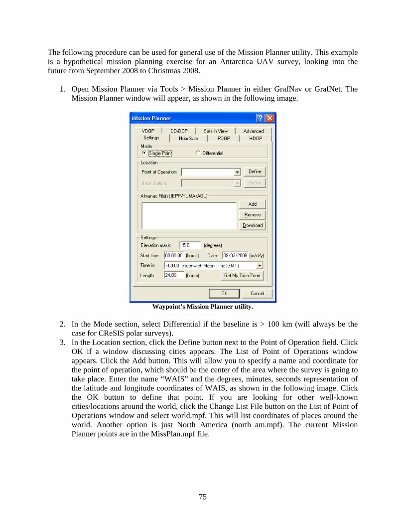
75

The following procedure can be used for general use of the Mission Planner utility. This example is a hypothetical mission planning exercise for an Antarctica UAV survey, looking into the future from September 2008 to Christmas 2008.

1. Open Mission Planner via Tools > Mission Planner in either GrafNav or GrafNet. The Mission Planner window will appear, as shown in the following image.

Waypoint’s Mission Planner utility.

2. In the Mode section, select Differential if the baseline is > 100 km (will always be the

case for CReSIS polar surveys). 3. In the Location section, click the Define button next to the Point of Operation field. Click

OK if a window discussing cities appears. The List of Point of Operations window appears. Click the Add button. This will allow you to specify a name and coordinate for the point of operation, which should be the center of the area where the survey is going to take place. Enter the name “WAIS” and the degrees, minutes, seconds representation of the latitude and longitude coordinates of WAIS, as shown in the following image. Click the OK button to define that point. If you are looking for other well-known cities/locations around the world, click the Change List File button on the List of Point of Operations window and select world.mpf. This will list coordinates of places around the world. Another option is just North America (north_am.mpf). The current Mission Planner points are in the MissPlan.mpf file.

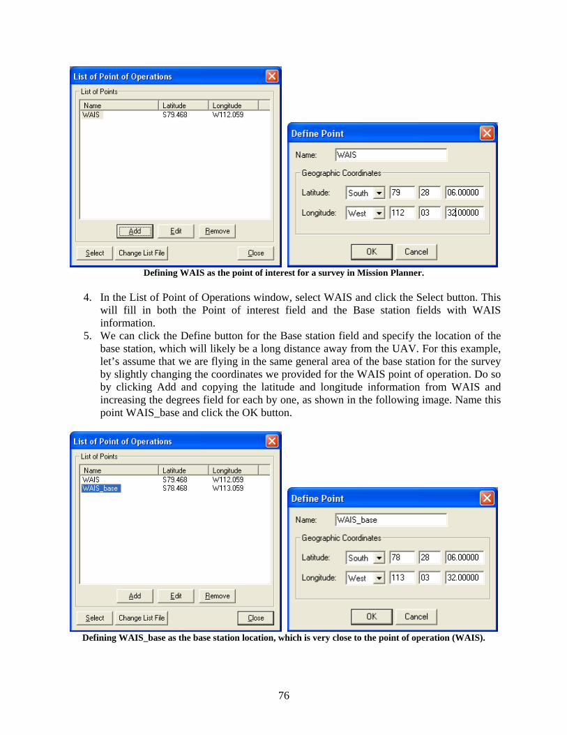
76

Defining WAIS as the point of interest for a survey in Mission Planner.

4. In the List of Point of Operations window, select WAIS and click the Select button. This

will fill in both the Point of interest field and the Base station fields with WAIS information.

5. We can click the Define button for the Base station field and specify the location of the base station, which will likely be a long distance away from the UAV. For this example, let’s assume that we are flying in the same general area of the base station for the survey by slightly changing the coordinates we provided for the WAIS point of operation. Do so by clicking Add and copying the latitude and longitude information from WAIS and increasing the degrees field for each by one, as shown in the following image. Name this point WAIS_base and click the OK button.

Defining WAIS_base as the base station location, which is very close to the point of operation (WAIS).

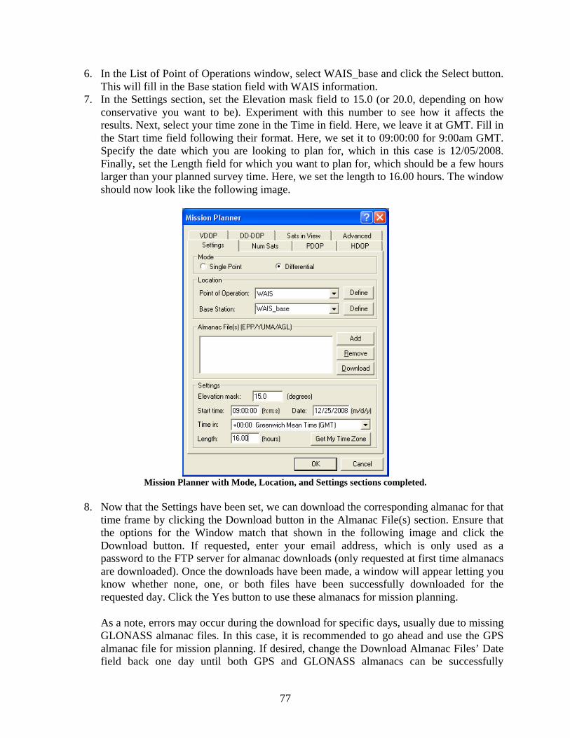
77

6. In the List of Point of Operations window, select WAIS_base and click the Select button. This will fill in the Base station field with WAIS information.

7. In the Settings section, set the Elevation mask field to 15.0 (or 20.0, depending on how conservative you want to be). Experiment with this number to see how it affects the results. Next, select your time zone in the Time in field. Here, we leave it at GMT. Fill in the Start time field following their format. Here, we set it to 09:00:00 for 9:00am GMT. Specify the date which you are looking to plan for, which in this case is 12/05/2008. Finally, set the Length field for which you want to plan for, which should be a few hours larger than your planned survey time. Here, we set the length to 16.00 hours. The window should now look like the following image.

Mission Planner with Mode, Location, and Settings sections completed.

8. Now that the Settings have been set, we can download the corresponding almanac for that

time frame by clicking the Download button in the Almanac File(s) section. Ensure that the options for the Window match that shown in the following image and click the Download button. If requested, enter your email address, which is only used as a password to the FTP server for almanac downloads (only requested at first time almanacs are downloaded). Once the downloads have been made, a window will appear letting you know whether none, one, or both files have been successfully downloaded for the requested day. Click the Yes button to use these almanacs for mission planning.

As a note, errors may occur during the download for specific days, usually due to missing GLONASS almanac files. In this case, it is recommended to go ahead and use the GPS almanac file for mission planning. If desired, change the Download Almanac Files’ Date field back one day until both GPS and GLONASS almanacs can be successfully

78

downloaded. Attempting the same day multiple times may also end up in better GLONASS FTP connections. Images showing these screens also follow.

Almanac file download options.

Screens showing the downloading of almanacs (left), and the result (1/2 in this case, as GLONASS failed).

9. Select Bar graph under Num Sats, PDOP, and DD-DOP tabs. Select None under VDOP

and HDOP tabs. Select Satellite lock plot under Sats in View tab. Adjust Advanced tab to your liking. These are all for displaying the results for the mission plan.

10. Click the OK button to begin mission planning. A window may come up letting you know that the GPS almanac that you are using is “out of date” by the number of days between the downloaded almanac date and the desired mission planning date. For planning for future and past dates, click Yes to continue. For current or next day planning, click No to get the most updated almanac files possible.

79

11. Analyze the plots to determine when not to fly. The plots for this example are shown below. Those of most importance are the Num Sats Plot, the Satellites in View Plot, the DD-DOP Plot, and the PDOP Plot.

The DD-DOP plot shows results of satellites visible to both the base station and point of operation (roving receiver). It is recommended to NOT survey during times which exhibit large spans of yellow color, or red colors. The PDOP plot shows accuracy effects on XYZ position. It is recommended to NOT survey during times which contain large spikes in either the questionable or unacceptable ranges. Additionally, the Num Sats and Satellites in View plots are different ways at looking at the same issue: number of visible satellites during the planning time frame. It is recommended to NOT survey during times (especially for long periods of time) when there are fewer than 6 satellites visible. Large thick red lines in the Satellites in View Plot are indicators of a large number of cycle slips for specific satellites. For example, satellites 5 and 25 will be useless during that time, as they are red. Furthermore, both PDOP and DD-DOP plots show that between 11:30pm and 12:00am for Christmas are times when surveys should not be made (yellow and red spikes). Changing the Elevation mask field also greatly affects results. Lower this mask to be less conservative and regenerate the results to see if problem areas have gone away. These guidelines can be generally followed to analyze when and when not to fly. See the other Waypoint support documents for more information.

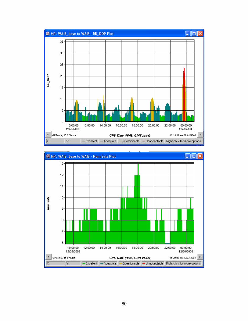
80

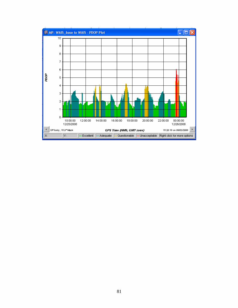
81