Waves User's Guide · 2004-09-20 · Waves User's Guide P/N 957-6148-00 (April 2001) page 3 2...

Waves User’s Guide

P/N 957-6148-00 (April 2001)

RD Instruments Acoustic Doppler Solutions

Table of Contents 1 Introduction....................................................................................................................................... 1

1.1 System Requirements.........................................................................................................................1 1.2 ADCP Requirements...........................................................................................................................2 1.3 ADCP Mounting Requirements ...........................................................................................................2 1.4 Software Installation............................................................................................................................2

2 Software Overview............................................................................................................................ 3 2.1 Background.........................................................................................................................................3 2.2 Using an ADCP as a Wave Gauge .....................................................................................................4 2.3 WavesPlan Overview..........................................................................................................................5 2.4 WavesMon..........................................................................................................................................6 2.5 WavesView .........................................................................................................................................8

3 Quick Start Guide ............................................................................................................................. 9 3.1 Quick Start – Collecting Self-Contained Data with WavesPlan.........................................................10 3.2 Quick Start - Collecting Real-Time Data with WavesMon .................................................................17 3.3 Quick Start - Process Data with WavesMon .....................................................................................25

4 Using WavesPlan............................................................................................................................ 31 4.1 Sample WavesPlan Command File ..................................................................................................34

5 Using WavesMon – Advanced Users............................................................................................ 36 5.1 Setting WavesMon’s View Menu Options .........................................................................................36 5.2 Collecting Real-Time Data with WavesMon – Advanced Users........................................................38

5.2.1 Setup Real-Time (Advanced) - Quick Tab ........................................................................................39 5.2.2 Setup Real-Time (Advanced) - Input Tab .........................................................................................40 5.2.3 Setup Real-Time (Advanced) - Output Tab.......................................................................................41 5.2.4 Setup Real-Time (Advanced) - Processing Tab................................................................................43 5.2.5 Setup Real-Time (Advanced) – ADCP Commands Tab ...................................................................47 5.2.6 Setup Real-Time (Advanced) – Expert 1 Tab ...................................................................................48 5.2.7 Setup Real-Time (Advanced) – Expert 2 Tab ...................................................................................50

5.3 Processing Raw ADCP Data – Advanced Users ..............................................................................52 5.3.1 Setup Playback (Advanced) – Quick setup Tab................................................................................53 5.3.2 Setup Playback (Advanced) – Input Tab...........................................................................................54

6 Using WavesView ........................................................................................................................... 55 7 Utility Programs .............................................................................................................................. 56 8 Waves Data Formats ...................................................................................................................... 57

8.1 WavesMon Input Data Formats ........................................................................................................57 8.2 WavesMon Output Data Formats......................................................................................................57 8.3 WaveView Input ................................................................................................................................58 8.4 WaveView Output .............................................................................................................................58

9 Frequently Asked Questions......................................................................................................... 59 10 Theory of Operation ....................................................................................................................... 61

10.1 Principles of ADCP Wave Measurement ..........................................................................................61 10.2 ADCP Performance as a Wave Gauge.............................................................................................61 10.3 Data Screening and Processing........................................................................................................62

10.3.1 Current Profile Averaging..................................................................................................................62 10.3.2 Discontinuities...................................................................................................................................63 10.3.3 Pressure Time Series .......................................................................................................................63 10.3.4 Velocity Time Series .........................................................................................................................63 10.3.5 Surface Track Time Series................................................................................................................63

10.4 Waves Processing ............................................................................................................................64 10.4.1 Height Spectrum ...............................................................................................................................64 10.4.2 Surface Track Height Spectrum........................................................................................................66 10.4.3 Velocity Height Spectrum..................................................................................................................66 10.4.4 Pressure Height Spectrum................................................................................................................67

10.4.5 Bias Removal....................................................................................................................................67 10.4.6 Cut-off Frequency Calculation...........................................................................................................67 10.4.7 Calculating Wave Number ................................................................................................................68 10.4.8 Translation for Velocity Spectrum .....................................................................................................68 10.4.9 Dispersion Relation...........................................................................................................................68 10.4.10 Directional Spectra .....................................................................................................................69 10.4.11 Maximum Likelihood Method (MLM) ..........................................................................................71 10.4.12 Iterative Maximum Likelihood Method (IMLM)............................................................................71 10.4.13 Linear Wave Theory ...................................................................................................................72 10.4.14 Translation for Pressure Spectrum.............................................................................................72

11 ADCP Waves Performance Specification..................................................................................... 73

List of Figures Figure 1. WavesPlan Screen.......................................................................................................... 5 Figure 2. WavesMon Display.......................................................................................................... 7 Figure 3. WaveView Display........................................................................................................... 8 Figure 4. WavesPlan Opening Screen ......................................................................................... 31 Figure 5. WavesPlan New Plan File Screen ................................................................................. 31 Figure 6. WavesPlan Choices Screen – Page 1 ........................................................................... 32 Figure 7. WavesPlan Choices Screen – Page 2 ........................................................................... 33 Figure 8. WavesMon View Options Dialog ................................................................................... 36 Figure 9. Setup Real-Time (Advanced) - Quick Tab ..................................................................... 39 Figure 10. Setup Real-Time (Advanced) - Input Tab ...................................................................... 40 Figure 11. Setup Real-Time (Advanced) - Output Tab.................................................................... 41 Figure 12. Setup Real-Time (Advanced) - Processing Tab............................................................. 43 Figure 13. Setup Real-Time (Advanced) – ADCP Commands Tab................................................. 47 Figure 14. Setup Real-Time (Advanced) – Expert 1 Tab ................................................................ 48 Figure 15. Setup Real-Time (Advanced) – Expert 2 Tab ................................................................ 50 Figure 16. Setup Playback (Advanced) – Quick setup Tab............................................................. 53 Figure 17. Setup Playback (Advanced) – Input Tab ....................................................................... 54 Figure 18. Height Spectrum – Velocity Array.................................................................................. 64 Figure 19. Height Spectrum – Echo Intensity ................................................................................. 65 Figure 20. Height Spectrum – Pressure Sensor ............................................................................. 65 Figure 21. Wave Height Spectrum.................................................................................................. 65 Figure 22. Average Directional Spectrum....................................................................................... 70 Figure 23. Directional Spectrum..................................................................................................... 70

List of Tables Table 1: Commands File Created with WavesPlan ..................................................................... 35 Table 2: File Naming Conventions .............................................................................................. 57

Waves User's Guide

P/N 957-6148-00 (April 2001) page 1

Acoustic Doppler Solutions

Waves User's Guide

1 Introduction The patented Waves software uses an innovative and powerful way to measure waves and currents at once. Using the Waves software with a RD Instruments WorkHorse ADCP allows you to distinguish waves from multi-ple directions and operate with less risk of loss or damage to the instrument. The ADCP measures velocity profiles, water level, and wave frequency-direction spectra simultaneously.

Waves applications include

• Coastal Protection and Engineering

• Port Design and Operation

• Environmental Monitoring

• Shipping Safety

1.1 System Requirements Waves requires the following:

• Windows 95®, Windows 98®, or Windows NT 4.0® with Ser-vice Pack 4 installed, Windows® 2000

• Pentium class PC 233 MHz (350 MHz or higher recommended)

• 32 megabytes of RAM (64 MB RAM recommended)

• 6 MB Free Disk Space plus space for data files (A large, fast hard disk is recommended)

• One Serial Port (two or more High Speed UART Serial Port rec-ommended)

Waves User's Guide

page 2 RD Instruments

• Minimum display resolution of 800 x 600, 256 color (1024 x 768 recommended)

• CD-ROM Drive

• Mouse or other pointing device

1.2 ADCP Requirements In order to use Waves, your Workhorse ADCP must meet the following cri-teria.

• A pressure gauge must be installed.

• The Workhorse ADCP must have version 16.xx firmware.

• The ADCP must have the Waves upgrade installed Initially for those who would like to collect Self-Contained waves data we recommend lots of memory (two 220 MB cards) and if necessary external battery packs. It is our goal to achieve a deployment length of at least 48 days using existing systems and the memory listed above.

1.3 ADCP Mounting Requirements The ADCP must be mounted as follows.

• Bottom mounted

• Upward facing

• Within 5 degrees of vertical RDI recommends using a gimbaled bottom mount to achieve the best per-formance (see the WorkHorse Installation Guide for recommended sources of bottom mounts).

1.4 Software Installation To install Waves, do the following.

a. Insert the compact disc into your CD-ROM drive and then follow the browser instructions on your screen. If the browser does not appear, complete Steps “b” through “d.”

b. Click the Start button, and then click Run.

c. Type <drive>:launch. For example, if your CD-ROM drive is drive D, type d:launch.

d. Follow the browser instructions on your screen.

Waves User's Guide

P/N 957-6148-00 (April 2001) page 3

2 Software Overview The basic principle behind wave measurement is that the wave orbital ve-locities below the surface can be measured by the highly accurate ADCP. The ADCP is bottom mounted, upward facing and has a pressure sensor for measuring tide and mean water depth. Time series of velocities are accu-mulated, and from these time series, velocity power spectra are calculated. To get a surface height spectrum, the velocity spectrum is translated to sur-face displacement using linear wave kinematics. The depth of each bin measured and the total water depth are used to calculate this translation.

To calculate directional spectra, phase information must be preserved. Each bin in each beam is considered an independent sensor in an array. The cross-spectrum is then calculated between each sensor and every other sen-sor in the array. The result is a cross-spectral matrix that contains phase information in the path between each sensor and every other sensor at each frequency band. The cross-spectrum at a particular frequency is linearly related to the directional spectrum at a particular frequency. By inverting this forward relation, we solve for the directional spectrum.

2.1 Background The use of Doppler sonar to measure ocean currents is by now well estab-lished, and is documented in the RDI publication Acoustic Doppler Current Profilers, Principles of Operation (RD Instruments, 1989). Conventional acoustic Doppler current profilers (ADCPs) typically use a Janus configura-tion consisting of four acoustic beams, paired in orthogonal planes, where each beam is inclined at a fixed angle to the vertical (usually 20 or 30 de-grees). The sonar measures the component of velocity projected along the beam axis, averaged over a range cell whose along-beam length is roughly half that of the acoustic pulse. Since the mean current is assumed horizon-tally uniform over the beams, its components can be recovered by subtract-ing the measured velocity from opposing beams. This procedure is rela-tively insensitive to contamination by vertical currents and/or unknown in-strument tilts (RD Instruments, 1989).

The situation regarding waves is more complicated. At any instant of time, the wave velocity varies across the array. As a result, except for waves that are highly coherent during their passage from one beam to another, it is not possible to separate the measured along-beam velocities into their horizon-tal and vertical components. However, the wave field is statistically steady in time and homogeneous in space, so that the cross-spectra of velocities measured at various range cells (either between different beams or along each beam) depend on wave direction. This fact allows us to apply array-processing techniques to estimate the frequency-direction spectrum of the waves. In other words, each depth cell of the ADCP can be considered an

Waves User's Guide


independent sensor that makes a measurement of one component of the wave field velocity. The ensemble of depth cells along the four beams con-stitutes an array of sensors from which magnitude and directional informa-tion about the wave field can be determined.

2.2 Using an ADCP as a Wave Gauge The ADCP can use its profiling ability (bins and beams) as an array of sen-sors. Because the ADCP can profile the water volume all the way to the surface, it can be mounted in much deeper water than a traditional pressure (PUV triplet) based device. Higher frequency waves attenuate more quickly with depth below the surface. The ADCP can measure much higher frequency waves than a PUV and do so in deeper water, because it can make measurements higher up in the water column. Additionally, the ADCP has many independent sensors (bins-beams) so even when sampling at a 2Hz sample rate the data is as quiet as if it had been sampled at 200Hz by a single point meter (example uses 25 bins and 4 beams).

To achieve the best possible solution for wave height spectrum, the height spectrum and the noise spectrum are fit to the bin-beam data using a least squares fit. In addition to the orbital velocity technique for measuring wave spectra, the ADCP can measure wave height spectra from its pressure sen-sor (with frequency/depth limitations) and from echo ranging the surface. Within the frequency range of the pressure sensor the pressure height spec-trum is an old reliable reference for data comparison. The surface track measurement of wave height is reliable most but not all of the time. The advantage of the surface track derived height spectrum is that it is a direct measurement of the surface and can measure wave energy at very high fre-quencies (higher than 0.9 Hz in some installations). Having three com-pletely independent measures of wave height spectrum that all agree very closely is a solid argument for data quality.

The directional spectrum is much truer and of higher quality than any sort of triplet (PUV, UVW, PRH) and is almost as good as large home-built ar-rays. The Maximum Likelihood Method used for inversion allows one to independently resolve the wave field in each direction. The full circle (360 degrees) is arbitrarily divided into as many slices as one chooses (up to 360 slices of 1 degree width). Because of this, the RDI directional spectra algo-rithm can resolve two separate swells arriving from different directions at similar frequency. This feat is impossible using traditional triplet algo-rithms.

The ADCP measures a sparse array and as such, it cannot achieve the aper-ture of expensive home built arrays, (e.g. Duck Is.). However, the aperture of the beams gives the ADCP a significant improvement in directional ac-curacy over single point measurements. A traditional triplet algorithm uses only the first three terms in a Fourier series so it can identify a single direc-

Waves User's Guide

P/N 957-6148-00 (April 2001) page 5

tional peak particularly at longer wavelengths. However, buoys, PUV’s, and other triplets cannot accurately represent the multiple directional peaks or even the true directional distribution.

In the ADCP wave algorithm there are many sensors giving an array with many degrees of freedom and some aperture. The Maximum Likelihood Method used to calculate the directional spectrum has a smearing kernal associated with the inversion. By using the Iterative Maximum Likelihood Method, the spreading of the directional spectrum can be corrected. The process is repeated until the directional spectrum converges to what the data actually supports. The spectrum will get narrower and sweep up direction-ally spread power into the peak as long as the measured data supports it. The result is a directional spectrum that more accurately represents the true directional distribution.

2.3 WavesPlan Overview WavesPlan is designed to set up a Self-Contained WorkHorse ADCP for collecting waves data. Specifically, WavesPlan will set the ADCP com-mands correctly for using Packets (see “Using WavesPlan,” page 31).

Figure 1. WavesPlan Screen

The WavesPlan screen shows you an overview of your setup and the resulting consequences of your deployment.

Waves User's Guide


2.4 WavesMon WavesMon is designed for real-time data collection and processing of wave data gathered by an ADCP. WavesMon can also be used for processing wave data gathered by a Self-Contained ADCP. For details on how to use WavesMon, see the “Quick Start Guide,” page 9 and “Using WavesMon – Advanced Users,” page 36.

WavesMon has two main modes of operation.

1. Packets: Packet mode was designed to reduce the amount of data that had to be stored for Self-Contained deployments. It is also geared toward reducing data for telemetry. The result is an order of magnitude reduction in data. Dramatically less data allows longer deployments and easier telemetry.

In packets mode, waves and current profiles are collected with inde-pendent sampling strategies. The current profile data is averaged, transformed, and output just like it would be if only currents were being collected. To reduce the amount of data that is produced by the waves sampling, only selected depth cells are preserved and out-put. Surface tracking is performed in the instrument reducing inten-sity profiles to a single value. The packets are kept small to aid in telemetry applications where bandwidth is small.

NOTE. Packet Mode is the default, and is set using the Auto Setup feature (see “Quick Start Guide,” page 9).

2. Ensembles: In ensemble mode, the software expects raw, un-transformed ensembles. The advantage of this is that all of the raw data is available for reprocessing. The ADCP is setup to collect un-averaged (i.e. single-ping), beam coordinate data, in bursts using the TB and TC commands. Averaging and transforming profile data in the software constructs the averaged current profiles. In addition, in this mode, the software can be setup to process data with a moving window. As an example, this allows a 20-minute data window to be processed every five minutes. The disadvantage is that the amount of data to record or move is huge. Typically, raw data consists of something over 500 bytes per ensemble. With hourly sampling, this amounts to approximately 30 Mbytes per day. For cabled, monitor-ing applications where frequent data updates are important and power/memory are not an issue; ensemble mode with a moving aver-age is the mode of choice.

NOTE. Ensemble Mode must be setup manually using the Advanced menus (see “Using WavesMon – Advanced Users,” page 36).

Waves User's Guide

P/N 957-6148-00 (April 2001) page 7

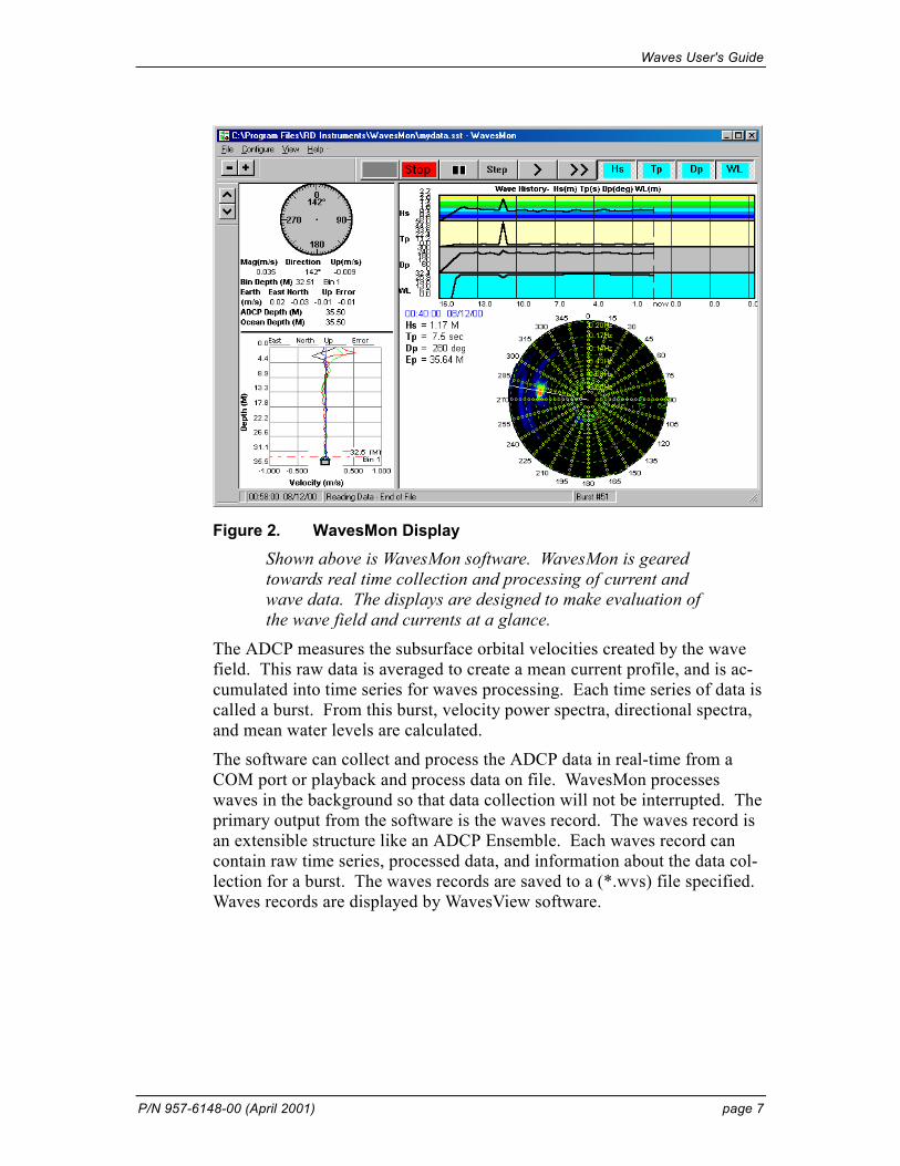
Figure 2. WavesMon Display

Shown above is WavesMon software. WavesMon is geared towards real time collection and processing of current and wave data. The displays are designed to make evaluation of the wave field and currents at a glance.

The ADCP measures the subsurface orbital velocities created by the wave field. This raw data is averaged to create a mean current profile, and is ac-cumulated into time series for waves processing. Each time series of data is called a burst. From this burst, velocity power spectra, directional spectra, and mean water levels are calculated.

The software can collect and process the ADCP data in real-time from a COM port or playback and process data on file. WavesMon processes waves in the background so that data collection will not be interrupted. The primary output from the software is the waves record. The waves record is an extensible structure like an ADCP Ensemble. Each waves record can contain raw time series, processed data, and information about the data col-lection for a burst. The waves records are saved to a (*.wvs) file specified. Waves records are displayed by WavesView software.

Waves User's Guide


2.5 WavesView WaveView is geared toward analysis and presentation of processed wave data created by the software program WaveMon. WaveView allows you to view time series and search for interesting events or wave climate. The software reads files containing wave records (*.wvs). The wave record is an extensible structure like an ADCP Ensemble. Each wave record can contain raw time series, processed data, and information about the data col-lection for a burst. For details on how to use WavesView, see “Using WavesView,” page 55.

Use the File menu to load a wave record (*.wvs) file. WaveView allows you to zoom, average, and animate wave height spectra, and directional spectra. Any of the displays can be saved to text files, saved as a bitmap or Portable Network Graphic (PNG), and printed.

Figure 3. WaveView Display

WaveView provides a big picture view of the wave climate as well as details of individual height spectra and directional spectra. Time-series of significant wave height, peak period, peak direction, water level, and height spectra make it easy to find significant events.

Waves User's Guide

P/N 957-6148-00 (April 2001) page 9

3 Quick Start Guide The Quick Start Guide is split into the following sections.

• How to collect self-contained data using WavesPlan (see “Quick Start – Collecting Self-Contained Data with WavesPlan,” page 10).

• How to collect real-time data using WavesMon (see “Quick Start - Collecting Real-Time Data with WavesMon,” page 17).

• Processing raw ADCP data using WavesMon (see “Quick Start - Process Data with WavesMon,” page 25).

NOTE. The Quick Start Guides are designed to use the Auto Setup feature. Auto Setup will set the ADCP to collect Packet data.

Waves User's Guide


3.1 Quick Start – Collecting Self-Contained Data with WavesPlan WavesPlan is designed to create a command file that will be used to set up a Self-Contained WorkHorse ADCP for collecting waves data.

Step 1. Start WavesPlan. At the RDI Plan dialog, click New to create a new command file or select a *whp file to open.

Use this area for notes.

Waves User's Guide

P/N 957-6148-00 (April 2001) page 11

Step 2. Select the ADCP frequency in the WorkHorse ADCP Hardware Configuration section. Select whether you want Waves And Currents (recommended), Waves Only, or Currents Only. Enter the estimated dis-tance from the ADCP face to the surface in the Transducer Depth box. Click Next.


Waves User's Guide


Step 3. Enter your choices and review the Consequences (for more infor-mation, see “Using WavesPlan,” page 31). Click Next.


Waves User's Guide

P/N 957-6148-00 (April 2001) page 13

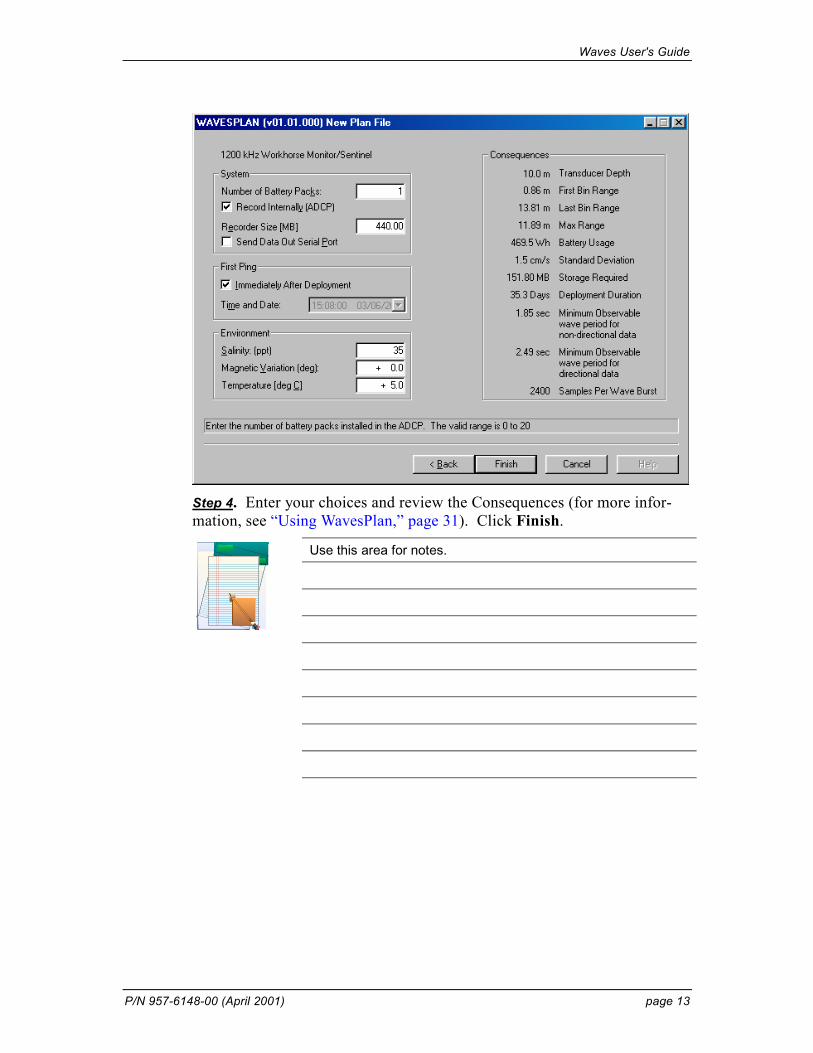
Step 4. Enter your choices and review the Consequences (for more infor-mation, see “Using WavesPlan,” page 31). Click Finish.


Waves User's Guide


Step 5. Name the WorkHorse Plan File and click Save.


Waves User's Guide

P/N 957-6148-00 (April 2001) page 15

Step 6. Start WinSC (see the WinSC User's Guide for details on how to use this program). On the Functions menu, click Import Planning File and select the command file created using WavesPlan.


Waves User's Guide


Step 7. Use the WinSC Wizard to send the deployment commands to the ADCP (see the WinSC User's Guide for details on how to use this pro-gram). Deploy and recover the ADCP. Use WinSC to recover the data. Use WavesMon to process the raw data into a Waves Record file (*.wvs) (see “Quick Start - Process Data with WavesMon,” page 25).


Waves User's Guide

P/N 957-6148-00 (April 2001) page 17

3.2 Quick Start - Collecting Real-Time Data with WavesMon WavesMon is designed for real-time data collection and processing of wave data gathered by an ADCP.

Photo courtesy of J. Bornhoeft.

Step 1. Connect the ADCP and computer as shown in your ADCP User's Guide. If you have not already installed the Waves and DumbTerm pro-grams do so as outlined in “Software Installation,” page 2. Run DumbTerm to verify the ADCP is functioning properly (see the RDI Tools User's Guide). Mount the ADCP in the bottom mount at the desired depth (see the WorkHorse Installation Guide).


Waves User's Guide


Step 2. Start WavesMon. On the File menu, click New Setup. At the Choose a realtime or playback setup dialog, choose Realtime. Click OK.


Waves User's Guide

P/N 957-6148-00 (April 2001) page 19

Step 3. On the Save Setup As dialog, name the Setup file something mean-ingful. The output data files (see next page) will be tied to the setup file name and path. Click Open.


Waves User's Guide


Step 4. Click Auto Setup.


Waves User's Guide

P/N 957-6148-00 (April 2001) page 21

Step 5. Select the ADCP’s System Frequency. Click the Choose Com button to select the ADCP communication settings. WavesMon will auto-matically test the communication settings. Try to select the fastest Baud rate that can reliably communicate with the ADCP.

Enter the ADCP Environment information. The Depth is the estimated depth of water from the ADCP face to the surface. The Altitude is the dis-tance of the ADCP face from the seafloor. Enter the Magnetic Variation to correct the data from magnetic north to true north. Click Next.


Waves User's Guide


Step 6. Set the Waves and Currents Sampling parameters. When you are done, click Finish.

Waves Sampling – enter the Burst Duration and the Time Between start of Bursts. The recommended setting is 20 minutes Burst Duration with 60 minutes Time Between start of Bursts. Currents Sampling – enter the Time Between Averages Ensembles. The recommended setting is 5 minutes. Start Time – Click Now to start pinging as soon as the commands are sent, or Later to delay pinging. To make data analysis easier, it is recommended to delay the start time until the hour mark.


Waves User's Guide

P/N 957-6148-00 (April 2001) page 23

Step 7. Review the Pre Deployment Summary. To save the Pre Deploy-ment Summary, click Save Summary. Click OK.


Waves User's Guide


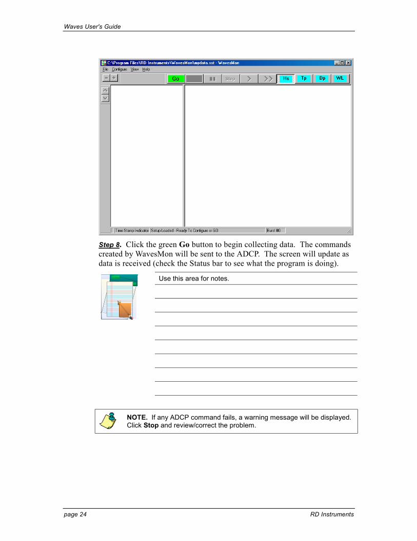
Step 8. Click the green Go button to begin collecting data. The commands created by WavesMon will be sent to the ADCP. The screen will update as data is received (check the Status bar to see what the program is doing).


NOTE. If any ADCP command fails, a warning message will be displayed. Click Stop and review/correct the problem.

Waves User's Guide

P/N 957-6148-00 (April 2001) page 25

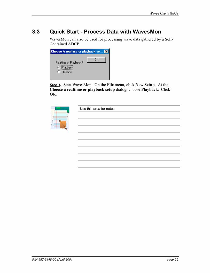
3.3 Quick Start - Process Data with WavesMon WavesMon can also be used for processing wave data gathered by a Self-Contained ADCP.

Step 1. Start WavesMon. On the File menu, click New Setup. At the Choose a realtime or playback setup dialog, choose Playback. Click OK.


Waves User's Guide


Step 2. On the Save Setup As dialog, name the Setup file something mean-ingful. The output data files (see next page) will be tied to the setup file name and path. Click Open.


Waves User's Guide

P/N 957-6148-00 (April 2001) page 27

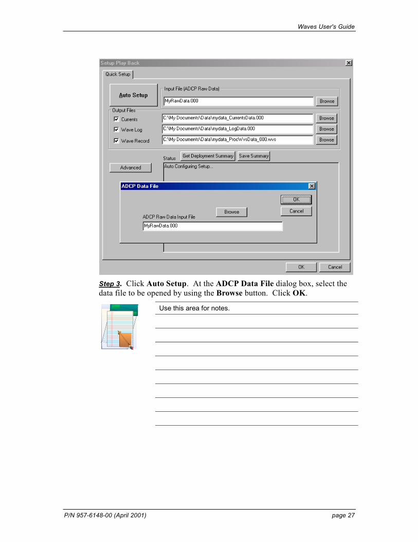
Step 3. Click Auto Setup. At the ADCP Data File dialog box, select the data file to be opened by using the Browse button. Click OK.


Waves User's Guide


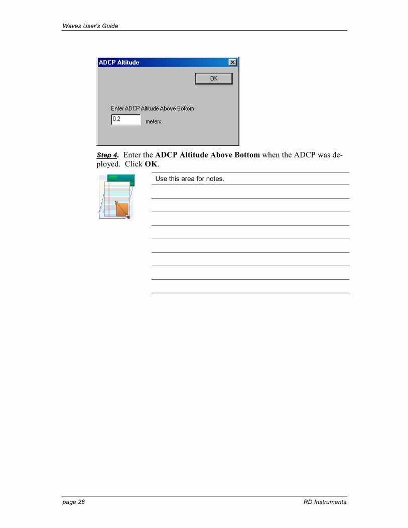
Step 4. Enter the ADCP Altitude Above Bottom when the ADCP was de-ployed. Click OK.


Waves User's Guide

P/N 957-6148-00 (April 2001) page 29

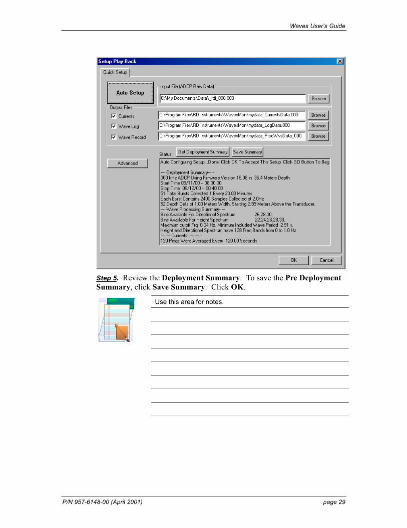
Step 5. Review the Deployment Summary. To save the Pre Deployment Summary, click Save Summary. Click OK.


Waves User's Guide


Step 6. Click the green Go button. When the processing is done, there will be a “Reading Data - End of File” message on the status bar.


Waves User's Guide

P/N 957-6148-00 (April 2001) page 31

4 Using WavesPlan WavesPlan will build an ADCP command file based on your deployment depth and sampling strategy. This file will be saved as a *.whp file.

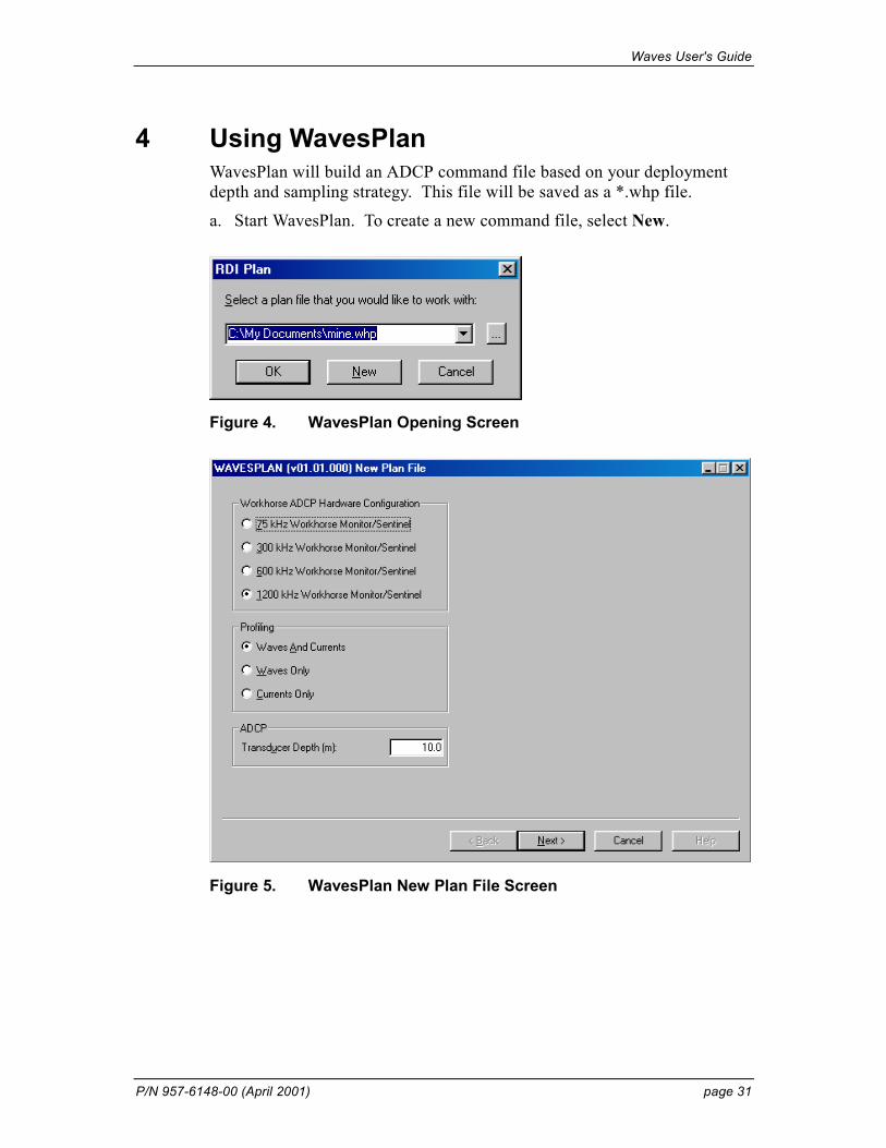
a. Start WavesPlan. To create a new command file, select New.

Figure 4. WavesPlan Opening Screen

Figure 5. WavesPlan New Plan File Screen

Waves User's Guide


b. Select the ADCP frequency.

c. Select the Profiling type. If you select Waves And Currents both the Current (W-commands) and the Waves (H-commands) will be setup.

d. Enter the Transducer Depth.

e. Click the Next button.

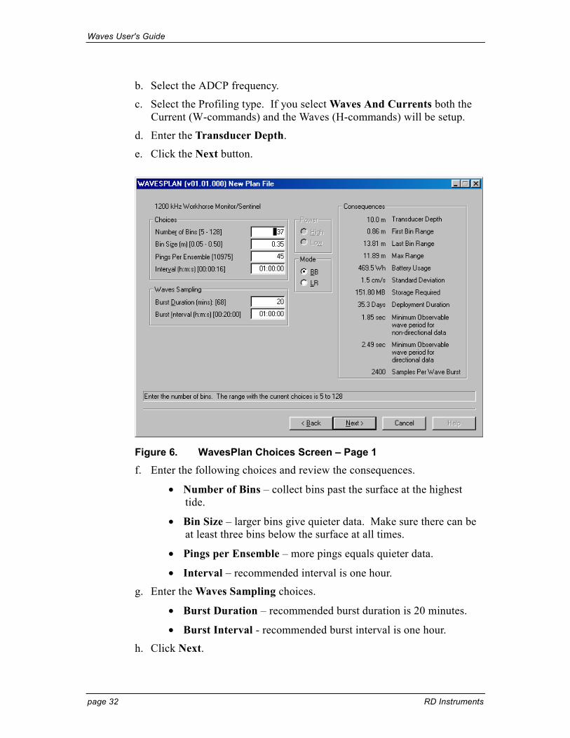
Figure 6. WavesPlan Choices Screen – Page 1 f. Enter the following choices and review the consequences.

• Number of Bins – collect bins past the surface at the highest tide.

• Bin Size – larger bins give quieter data. Make sure there can be at least three bins below the surface at all times.

• Pings per Ensemble – more pings equals quieter data.

• Interval – recommended interval is one hour. g. Enter the Waves Sampling choices.

• Burst Duration – recommended burst duration is 20 minutes.

• Burst Interval - recommended burst interval is one hour. h. Click Next.

Waves User's Guide

P/N 957-6148-00 (April 2001) page 33

Figure 7. WavesPlan Choices Screen – Page 2 i. Enter the System information

• Number of Battery Packs – enter the number of battery packs in your ADCP. The WorkHorse Sentinel ADCP holds one battery pack. The External Battery Pack can hold up to two batteries. External Battery Packs can be strung together to increase the number of available batteries.

• Record Internally – this must be selected for self-contained de-ployments.

• Recorder Size – enter the total size of your ADCP’s recorder. j. Check the Immediately After Deployment box to begin pinging as

soon as the ADCP receives the commands or enter a Time and Date to delay pinging. It is recommended to delay pinging so the ADCP starts on the hour.

k. Enter the Environment data.

• Salinity at the transducer head.

• Magnetic Variation at the deployment site.

• Temperature at the transducer head. l. When you have enter all of your choices review the Consequences. If

you are satisfied with them, click the Finish button.

Waves User's Guide


4.1 Sample WavesPlan Command File Once you have entered all of your choices using WavesPlan and saved the file, you can view the command file using any text editor. Lines beginning with a semicolon (;) are comments. CR1 CF11101 EA00000 EB00000 ED00100 ES35 EX11111 EZ1111111 TE01:00:00.00 TP01:20.00 WB0 WD111100000 WF0044 WN037 WP00045 WS0035 WV170 HB05 HD111000000 HR01:00:00.00 HT00:00:00.50 HP2400 WA255 CK CS ;Temperature = 5.00 ;Frequency = 1228800 ;BatteryPacks = 1 ;RecorderSize = 440.00

The commands shown in Table 1, page 35 explain each command set or added by WavesPlan. These commands directly affect the range of the ADCP, standard deviation (accuracy) of the data, and battery usage. Table 1, page 35 explains the commands used in the sample command file. This command file uses the default settings for a 1200kHz ADCP.

Waves User's Guide

P/N 957-6148-00 (April 2001) page 35

Table 1: Commands File Created with WavesPlan Command Choices Description

CR1 Sets factory defaults This is the first command sent to the ADCP to place it in a “known” state.

CF11101 Flow control Record data internally on the PC card recorder.

EA00000 Heading alignment Use beam-3 as the heading alignment.

EB00000 Heading bias Magnetic variation.

ED00100 Transducer depth Manually set depth of the transducer to 10 me-ters. The ED-command will be used only if the pressure sensor fails.

ES35 Salinity Salinity of water is set to 35 (saltwater).

EX11111 Coordinate transformations Sets Earth coordinates, use tilts, allow 3-beam solutions, and allow bin mapping to ON.

EZ1111111 Sensor source Calculate speed of sound from readings, use pressure sensor, internal compass, internal tilt sensor, and transducer temperature sensor.

TE01:00:00.00 Time per ensemble Ensemble interval is set to one hour.

TP01:20.00 Time between pings Plan automatically sets the time between pings to spread the pings evenly throughout the en-semble.

WB0 Bandwidth mode Sets the ADCP to the Broadband mode.

WD111 100 000 Data out Sets the ADCP to collect velocity, correlation magnitude, echo intensity, and percent-good data. Status data is not used.

WF0044 Blank after transmit Moves the location of the first depth cell 44 cm away from the transducer head.

WN037 Number of depth cells Number of bins is set to 37.

WP00045 Pings per ensemble The ADCP will ping 45 times per ensemble.

WS0035 Depth cell size Bin size is set to 0.35 meters.

WV170 Ambiguity velocity Sets the maximum relative horizontal velocity between water-current speed and WorkHorse speed to 170 cm/s.

HB05 Bins for Wave Processing Set the number of automatically chosen bins for doing Directional Wave Spectra.

HD111000000 Waves Data Out Select the data output in the Waves Packet Structure.

HR01:00:00.00 Time Between Wave Re-cords

Set the maximum interval between the start of each wave record.

HT00:00:00.50 Time Between Wave Re-cord Pings

Set the maximum interval between each wave ping.

HP2400 Waves Pings per Wave Record

Set the number of pings per wave record.

WA255 False Target Threshold Sets a false target (fish) filter (255 disables this filter).

CK Keep parameters as user defaults

If power is lost and then restored, all commands will be restored as last sent. Sent right before the CS-command.

CS Start pinging Last command sent to begin collecting data.

Waves User's Guide


5 Using WavesMon – Advanced Users The easiest way to collect and process data with WavesMon is to use the Auto Setup feature (see “Quick Start Guide,” page 9). In some cases, it may be necessary to use the advanced features.

5.1 Setting WavesMon’s View Menu Options The View menu allows you to tailor the displays to your needs. Unlike the other menus, the view menu can be changed while data collection is under-way. The only item in the View menu that cannot be changed while run-ning is the number of hours of history to display.

CAUTION. Leaving the view menu dialog open for an extended time period will eventually block the data collection. Therefore, it is recommended that this dialog be closed (OK or Cancel) after changes have been made.

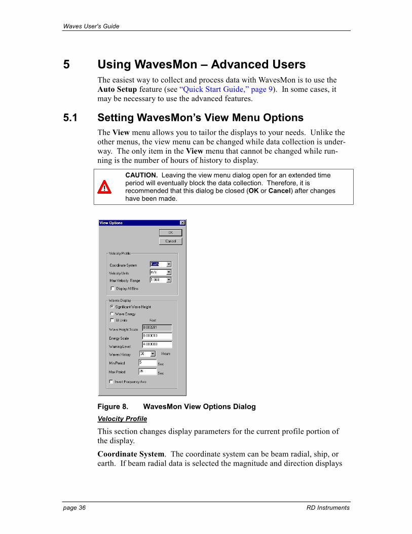
Figure 8. WavesMon View Options Dialog Velocity Profile

This section changes display parameters for the current profile portion of the display.

Coordinate System. The coordinate system can be beam radial, ship, or earth. If beam radial data is selected the magnitude and direction displays

Waves User's Guide

P/N 957-6148-00 (April 2001) page 37

will be invalid. The selection of beam coordinates in the profile display is intended for trouble shooting purposes only.

Velocity Units. The velocity units can be displayed in knots, ft/s, and meters/s.

Maximum Velocity Range. The default velocity scaling can be set here. At any time the velocity scale can be changed using the + and - buttons on the toolbar or the + - keys on the keyboard. The value set by this control is saved as the default so the next time the program is run it will begin with this scaling.

Display All Bins. Under normal operation, the profile display clips at the surface. If you would like to see bins beyond the surface, select this check box and the display will show all of the bins collected. Waves Display

This section changes display parameters for the waves displays.

Significant Wave Height. This buttons allow you to choose significant wave height to be displayed in the wave history plot. Hs or significant wave height is the square root of 4 times the integral under the power spec-trum. This is equivalent to H1/3, or the average of the 1/3 largest wave.

SI Units. Selecting this check box displays wave data in meters. Other-wise, the units are feet. Based on this the wave height scale factor is chosen and displayed. The data is stored internally in mm.

Warning Level. The warning level sets the color scale on the wave height history plot. Whatever value is set here will be scaled to be warning red. For example, if a harbor authority decided that eight feet of significant wave height was dangerous and should catch the attention of the person monitoring the software then they would set the warning level to seven or eight.

Wave History. If this is set to eight hours the wave history plot will dis-play the last eight hours of significant wave height data. The plot will grow progressively from the left until eight hours is collected. The display will automatically wrap after this time, always giving the most recent eight hours of data. The display shows the data in time regardless of the number of bursts that are contained in an hour. This plot is reset if the data collec-tion is stopped.

Min/Max. Period. The minimum and maximum period that are displayed by the directional spectra plot are set by these controls.

Invert Frequency Axis. The frequency period axis can be inverted for the directional spectra polar plot if this is your preference. The standard way places long wave lengths on the inside of the polar plot. Selecting Inverted places long wave lengths on the outside.

Waves User's Guide


5.2 Collecting Real-Time Data with WavesMon – Advanced Users a. Start WavesMon.

b. On the File menu, click New Setup. At the Choose a realtime or play-back setup dialog, choose Realtime. Click OK.

c. On the Save Setup As dialog, name the Setup file something meaning-ful. The output data files will be tied to the setup file name and path. Click Open.

d. On the Setup Real-Time Operation screen, click the Advanced button. The WavesMon Advanced tabs allows you to change how the software operates. These changes are saved to the *.sst setup files when you click OK on the dialog box. For details on how to set each tab, see the following sections.

• “Setup Real-Time (Advanced) - Quick Tab,” page 39

• “Setup Real-Time (Advanced) - Input Tab,” page 40

• “Setup Real-Time (Advanced) - Output Tab,” page 41

• “Setup Real-Time (Advanced) - Processing Tab,” page 43

• “Setup Real-Time (Advanced) – ADCP Commands Tab,” page 47

• “Setup Real-Time (Advanced) – Expert 1 Tab,” page 48

• “Setup Real-Time (Advanced) – Expert 2 Tab,” page 50 e. Select the View menu dialog (see “Setting WavesMon’s View Menu Op-

tions,” page 36) and choose the way you would like to see the displays. Click OK.

f. Click the GO button on the WavesMon toolbar. If results are not what you expected, click STOP and edit the Configure menus, then try again.

Waves User's Guide

P/N 957-6148-00 (April 2001) page 39

5.2.1 Setup Real-Time (Advanced) - Quick Tab

Figure 9. Setup Real-Time (Advanced) - Quick Tab The Quick Setup tab is the same screen as described in the “Quick Start - Collecting Real-Time Data with WavesMon,” page 17. Click the Auto Setup button to use this feature.

Waves User's Guide


5.2.2 Setup Real-Time (Advanced) - Input Tab

Figure 10. Setup Real-Time (Advanced) - Input Tab a. Click the Browse button to select a Com port and Baud rate. The soft-

ware will warn you if the setup you have chosen is not possible at the selected Baud rate.

b. To use Packet data (i.e. H-commands) check the Packet Collection Mode box to turn this option on.

Waves User's Guide

P/N 957-6148-00 (April 2001) page 41

5.2.3 Setup Real-Time (Advanced) - Output Tab

Figure 11. Setup Real-Time (Advanced) - Output Tab The Output tab allows you to select what files are output. Raw Data

Raw data can be saved to a file or COM port. Choose a valid path for any file options by clicking the Browse button.

NOTE. For Real-Time data collection, it is recommended that you select the Raw Data File box to save the ADCP raw data file.

Wave Parameters Log

The Waves Log File is a brief summary containing wave parameters (Hs, Tp, Dp, and averaged current profile data). Select any output options that you would like. Make sure you choose a path that exists for any file op-tions by clicking the Browse button.

If you check the Log File box, enter the Wave Log Format type. To view the formats, click the Show Format button.

Waves User's Guide


Processed Waves Data

Select the Processed Data check box to create a waves record file (*.wvs).

Check the Save Processed to Text Files to create an ASCII text file for each burst for each of the selected data types. The text file has a header de-scribing the contents of the file. These files can be loaded into Matlab or a spreadsheet for those who would like to process or analyze the data on their own. This option is recommended for users that would like to batch process text files for a whole data set. Currents Data

Select the Currents Data check box to create a data file with just the cur-rents data.

Waves User's Guide

P/N 957-6148-00 (April 2001) page 43

5.2.4 Setup Real-Time (Advanced) - Processing Tab

Figure 12. Setup Real-Time (Advanced) - Processing Tab In the What to Process section, the Process and Save check boxes let you choose what data to process and what data to save in the Waves Record (*.wvs) file. Note there is some dependency between the selected data types. One cannot do a Directional Spectrum if no Velocity Data was processed in the first place. Likewise, one cannot save a Surface Spec-trum if it was not processed to begin with. This allows the flexibility to process and display the data but just store spectra or wave parameters in the output file.

NOTE. Including Velocity, Surface, or Pressure Time Series in the saved Waves Record makes very large data files. If you do not require time series data to be output, do not select them in the What to Process, Save box (see Figure 12).

ADCP Environment

Transducer Altitude. If the Transducer Altitude is unchecked, it is as-sumed zero. If it is checked, one can enter an offset of the instrument from

Waves User's Guide


the bottom in cm. This helps get the bin locations correct if the instrument is mounted on another structure or is located significantly above the bottom.

Force Fixed Depth. If the box is unchecked, the software uses the instru-ment depth computed by the pressure sensor in each ensemble. These are averaged to calculate mean instrument depth. If no pressure sensor was available or the mean water depth was very large relative to tidal changes, or the pressure sensor failed, the nominal water depth can be forced to this value.

Depth Correction. The depth correction allows one to correct for an un-calibrated pressure sensor. If for example, the instrument has been sub-merged for a long time and the pressure sensor depth consistently reads lar-ger than the surface track depth, it is likely that the pressure sensor has drifted with time and needs to be zeroed at the surface again.

If the wave height spectra do not agree very closely between the velocity spectrum and the pressure or surface track spectrum, it may be because the pressure sensor is in error. An offset in the pressure measurement does not significantly affect the pressure spectrum, however, it does have an imme-diate affect on the velocity spectrum. The locations of the velocity bins be-low the surface are determined using the mean water depth from the pres-sure sensor. An overly large pressure sensor reading for depth will cause the velocity spectrum to be high as well. To correct for a pressure sensor reading 500 mm too high make the depth correction –500. ADCP heading

Force Fixed Heading. The heading is normally measured by the ADCP’s compass. If for some reason the instrument was mounted with a lot of steel nearby and the compass was not valid, the heading could be measured inde-pendently. Checking the box and entering a heading offset forces the soft-ware to use that heading always. The directional spectra algorithm must know the instruments heading to calculate wave direction.

Magnetic Variation. Enter the Magnetic Variation for your location in the world to have the direction information calculated relative to true North rather than magnetic North. How To Process

This section tells the software how to setup the ADCP. In real-time, some of this information is used to generate commands to be sent to the ADCP, in addition to guiding the software in its processing.

Samples/Burst. This is the number of ensembles accumulated into a burst for waves processing. Because of the statistical nature of ocean waves, it is recommended that this correspond to data spanning a range of 5 to 40 minutes.

Waves User's Guide

P/N 957-6148-00 (April 2001) page 45

Recommended Setting. Choose a Samples/Burst number so that more data is collected than required. For example, 2048 is the nearest power of two, 2400 samples allows some data to be potentially lost.

Time Between Bursts. WavesMon uses Time Between Bursts to handle real-time collection from an ADCP that is burst sampling. For example if an ADCP is collecting 20 minutes (2400 samples per burst) of data every hour on the hour, the time between bursts would be set to an hour. The ADCP time of first ping command would start the sampling on the next hour. Set the Time Between Bursts accurately or the software may treat good data as discontinuous. Set the burst duration exactly if continuously running. This creates the TB-command in the ADCP Commands tab.

Recommended Setting. A recommended setup is 20 minutes of data every hour on the hour.

FFT Length. The FFT Length control lets one choose the exact number of samples in the time series to be Fourier transformed. This must be a power of two and less than or equal to the Ensembles Per Burst. If an er-roneous value is chosen the software will pick the nearest power of two that is less than or equal to the value chosen and the Ensembles per Burst. This value would differ from the Ensembles per Burst if the ADCP were collecting bursts that are not a power two.

Recommended Setting. Set the Samples per Burst to 2400 (20 minutes of data) so that the current profile will have 3 averaging intervals 6 minutes long and the FFT will have 2048 samples.

Frequency Bands. The number of frequency bands must be a power of two and the maximum is half the FFT Length. Band averaging smoothes the data by averaging adjacent frequency band from the raw frequency spectrum. Band averaging also increases the number of degrees of freedom of the cross-spectral matrix because each frequency band is independent. Band averaging improves the results and speed of the directional spectra algorithm so it is recommended that at least some be done.

Recommended Setting. Using 128 Frequency Bands gives nice frequency resolution and still smoothes the data by a factor of square root eight. If very long waves are of interest, less band averaging (512 Frequency Bands) will give greater frequency resolution at these frequencies. Environments that see 20 second period waves and larger should use at least 256 Frequency Bands.

Frequency Thresholds. The Frequency threshold is calculated automati-cally for each height spectrum type (pressure, surface track, velocity). However, if for some reason the algorithm is not handling some set of envi-ronmental conditions properly you one can manually set the upper fre-quency cutoff. This becomes important to such calculations as significant

Waves User's Guide


wave height and determining the range of frequencies over which to search for a peak. See “Cut-off Frequency Calculation,” page 67 for more details.

Recommended Setting. The software attempts to calculate an upper cutoff frequency automatically, however if you would like to further limit the highest frequency you can force an upper threshold.

Number of Angles. The number of angles determines the angular resolu-tion of the directional spectrum. Dividing the full circle into 90 pie slices gives good resolution without overkill.

Recommended Setting. Set the number of angles to 90. This is the number of slices the 360-degree, full circle is divided into for the directional spectra calculation. You can use as high as 360 slices of one-degree width, however, the resulting spectrum does not change much, and there is four times as much data to move and plot. Less than 90 angle divisions will also work fine, however poor angular resolution will begin to degrade or smear the data.

Depth Cells Used For Waves

Height Spectrum Depth Cells. Many depth cells can be chosen, however, if high frequency data is of interest it is recommended that you choose depth cells nearer to the surface. Be sure that the highest depth cell is be-low the surface at low tide. If the instrument is mounted near an interfering object like a platform leg, depth cells can be chosen which skip this range.

Directional Spectrum Depth Cells. The direction spectrum algorithm must invert a sensor-by-sensor matrix at each frequency band. Empirically the algorithm appears to achieve good results with 3 or more depth cells. Theoretically, the depth cells should be chosen with some spread and farther up in the water column so that the array has as much aperture as possible. Be sure that you do not choose depth cells beyond the profiling range of the instrument.

Recommended Setting. It is recommended that you choose the Auto depth cell selection check box. If you want to select which bins are used manually this can be done as follows:

1. Choose Height Spectra Depth Cells that are nearer to the surface for better high frequency results. Make sure that the depth cells are not too close to the surface at low tide.

2. Choose three Directional Spectra Depth Cells that are higher in the water column. Less than three can cause the directional spectra algorithm to give poor results. More than three gives results that are more robust but has a dramatic affect on the speed of the algorithm. The point of diminishing returns is about three or four depth cells.

Waves User's Guide

P/N 957-6148-00 (April 2001) page 47

5.2.5 Setup Real-Time (Advanced) – ADCP Commands Tab

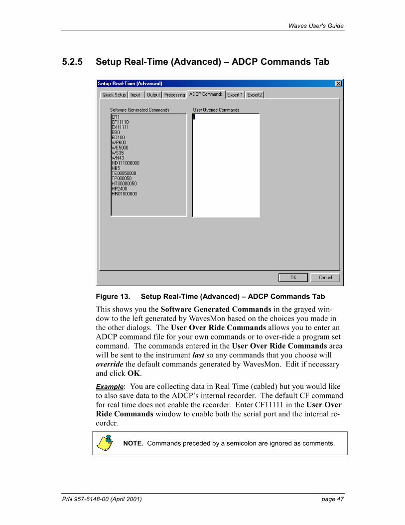
Figure 13. Setup Real-Time (Advanced) – ADCP Commands Tab This shows you the Software Generated Commands in the grayed win-dow to the left generated by WavesMon based on the choices you made in the other dialogs. The User Over Ride Commands allows you to enter an ADCP command file for your own commands or to over-ride a program set command. The commands entered in the User Over Ride Commands area will be sent to the instrument last so any commands that you choose will override the default commands generated by WavesMon. Edit if necessary and click OK.

Example: You are collecting data in Real Time (cabled) but you would like to also save data to the ADCP’s internal recorder. The default CF command for real time does not enable the recorder. Enter CF11111 in the User Over Ride Commands window to enable both the serial port and the internal re-corder.

NOTE. Commands preceded by a semicolon are ignored as comments.

Waves User's Guide


5.2.6 Setup Real-Time (Advanced) – Expert 1 Tab

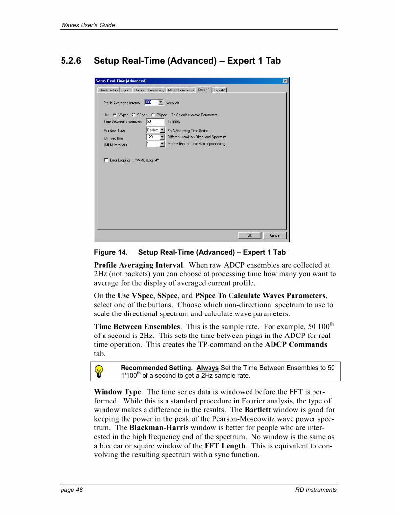
Figure 14. Setup Real-Time (Advanced) – Expert 1 Tab Profile Averaging Interval. When raw ADCP ensembles are collected at 2Hz (not packets) you can choose at processing time how many you want to average for the display of averaged current profile.

On the Use VSpec, SSpec, and PSpec To Calculate Waves Parameters, select one of the buttons. Choose which non-directional spectrum to use to scale the directional spectrum and calculate wave parameters.

Time Between Ensembles. This is the sample rate. For example, 50 100th of a second is 2Hz. This sets the time between pings in the ADCP for real-time operation. This creates the TP-command on the ADCP Commands tab.

Recommended Setting. Always Set the Time Between Ensembles to 50 1/100th of a second to get a 2Hz sample rate.

Window Type. The time series data is windowed before the FFT is per-formed. While this is a standard procedure in Fourier analysis, the type of window makes a difference in the results. The Bartlett window is good for keeping the power in the peak of the Pearson-Moscowitz wave power spec-trum. The Blackman-Harris window is better for people who are inter-ested in the high frequency end of the spectrum. No window is the same as a box car or square window of the FFT Length. This is equivalent to con-volving the resulting spectrum with a sync function.

Waves User's Guide

P/N 957-6148-00 (April 2001) page 49

The shorter the FFT Length the more spread or smeared the spectrum will be. Essentially, the end points of a finite time series cannot be reproduced without introducing high frequency harmonics. These higher frequency components are not representative of the content of the time series; they are representative of the envelope. A longer FFT has more data relative to the effects of the end points so it is less affected by this phenomenon. A Bart-lett or triangular window attempts to weight the data in the middle more and the ends less. This reproduces the true spectrum more accurately than using no window. There are many window types however almost any win-dow is substantially better than no window.

Recommended Setting. Any kind of window is a substantial improvement over none for reducing end effects in a finite data set. Bartlet and Blackman-Harris windows are available.

Dir Freq Bins. The number of output frequency bands for the directional spectrum can be selected independently from the number used for the non-directional spectrum.

Recommended Setting. For example, 64 directional frequency bands and 256 non-directional frequency bands provides good frequency resolution for non-directional spectrum and plenty of band averaging for the directional spectrum.

IMLM Iterations. The IMLM technique corrects MLM spectra for direc-tional spreading caused by the MLM algorithm. It makes narrower more true to life directional spectra. The point of diminishing returns is about 3 IMLM iterations. Each iteration makes the processing take longer. Three iterations or more appears to produce a directional spectrum that converges with the data. That is to say, that 20 iterations yields a spectrum that is about the same as 3, yet three iterations is a huge improvement over the original MLM estimate (0 iterations). For more about MLM and IMLM see the Directional Spectra Algorithm.

Recommended Setting. Choose one IMLM iterations for best results. Each iteration makes the processing take longer. One iteration appears to produce a directional spectrum that converges with the data.

Error Logging to WMErrLog.txt. This will create an error log text file that helps in troubleshooting Waves setup. This diagnostic tool outputs in-formation about why waves data was screened and how often.

Display Dirspec in Power x Power. Directional spectrum is stored and displayed as square root spectrum so its total dynamic range is not so large. To output the directional spectrum in units of power, select this option. This is required to have the integrated direction/spectrum equal the non-directional power spectrum.

Waves User's Guide


5.2.7 Setup Real-Time (Advanced) – Expert 2 Tab

Figure 15. Setup Real-Time (Advanced) – Expert 2 Tab Data Screening

STD Threshold – Velocity and surface time series are screened before be-ing Fourier transformed. The primary screening is the wild point editor. It throws out and interpolates data points that are more than “n” standard de-viations away from the mean. The STD Threshold default is set to four.

Percent Good – If more data is rejected than set by the Pct. Good Thresh-old, then waves processing will not be performed.

NOTE. Minimum, Maximum, and Max Change are not used.

Max Ensemble Timing Deviation – In the event that data communications is unreliable, the software will accept deviations in the time stamps for in-dividual ensembles (for example, some data was lost). If large gaps (greater than 5 seconds) occur in the data, it will still reject the data as being discon-tinuous. This keeps the waves processing from averaging or “FFTing” data from two different time frames yet allows small glitches.

Waves User's Guide

P/N 957-6148-00 (April 2001) page 51

Use File Buffer For Data – Use this option if your PC has limited RAM memory. This will slow down processing. It is recommended that the PC RAM be upgraded rather than using the file buffer.

Small Wave Screening Frequency – When very small waves are being measured, the orbital velocity spectrum can be biased by the noise floor of the measurement at very low frequencies. To avoid this problem, the pres-sure derived spectrum is used to represent very long waves in the wave height spectrum. Misc Number of Bursts to Process – The software will process exactly this many bursts, than stop. This can be used to batch process data.

Omega Cal. – Reserved for future use.

Save Surface Direction – If surface track data is collected and text output files are chosen (see “WavesMon Output Data Formats,” page 57), the peak directions based on surface spectra are output to a file named SurfDir-Spec.txt. The surface direction is used as a secondary directional reference for long mono-directional waves with good signal-to-noise.

Save Images – Saves the WavesMon screens (currents to the left, waves to the right) every time they are updated with new data, to PNG image files. This makes displaying of real-time data images on a web page or animation convenient.

Correct for Currents – Uses the mean currents to correct the wave spectra for the effects of currents. A Doppler shifted dispersion relation is used to calculate wave number “k.” This should be applied if the currents near the measurement exceed 0.75 m/s. Advanced Processing

Reserved for future use. Static Select the Simulate Directional Spectrum box to simulate a directional spectrum. Make sure that a Forced Depth and Forced Heading are used (see “Setup Real-Time (Advanced) - Processing Tab,” page 43).

Waves User's Guide


5.3 Processing Raw ADCP Data – Advanced Users Raw ADCP data is processed using WavesMon to create the Waves Record (*.wvs) file. In real-time, raw data is saved and processed. In Playback, previously recorded raw data is processed.

Raw data can come from a Com Port in real-time (see “Collecting Real-Time Data with WavesMon – Advanced Users,” page 38) and saved by WavesMon. Raw data files created by a self-contained ADCP can be stored separately on the ADCP recorder, downloaded to a PC file, and saved by WavesMon during processing.

NOTE. A sample raw data file is included on the Waves CD. It is not copied to your hard drive during software installation.

a. Start WavesMon.

b. On the File menu, click New Setup. At the Choose a realtime or play-back setup dialog, choose Playback. Click OK.

c. On the Save Setup As dialog, name the Setup file something meaning-ful. The output data files will be tied to the setup file name and path. Click Open.

d. On the Setup Playback Operation screen, click the Advanced button. The WavesMon Advanced tabs allows you to change how the software operates. These changes are saved to the *.sst setup files when you click OK on the dialog box. For details on how to set each tab, see the following sections.

• “Setup Playback (Advanced) – Quick setup Tab,” page 53

• “Setup Playback (Advanced) – Input Tab,” page 54

• “Setup Real-Time (Advanced) - Output Tab,” page 41

• “Setup Real-Time (Advanced) - Processing Tab,” page 43



NOTE. The functions on the Output, Processing, Expert 1, and Expert 2 tabs are the same as the real time setup tabs.

e. Select the View menu dialog (see “Setting WavesMon’s View Menu Op-tions,” page 36) and choose the way you would like to see the displays. Click OK.

Waves User's Guide

P/N 957-6148-00 (April 2001) page 53

f. Click the GO button on the WavesMon toolbar. If results are not what you expected, click STOP and edit the Configure menus, then try again.

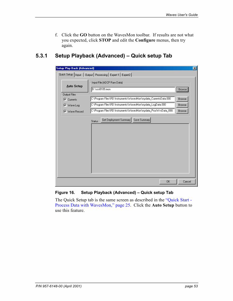
5.3.1 Setup Playback (Advanced) – Quick setup Tab

Figure 16. Setup Playback (Advanced) – Quick setup Tab The Quick Setup tab is the same screen as described in the “Quick Start - Process Data with WavesMon,” page 25. Click the Auto Setup button to use this feature.

Waves User's Guide


5.3.2 Setup Playback (Advanced) – Input Tab

Figure 17. Setup Playback (Advanced) – Input Tab Input Data From – choose between File and Com Port. Normally, File is selected. The Com Port setting is a special read only mode that sends no commands out (for use with a Sea Wave).

Input ADCP Data from File – Use the Browse button to select the data file.

Data Type/File Size – The Data Type will show Ensembles if the data file has raw ensemble data or Packets if the raw data file uses Packet data.

Skip N Bytes Into File – Use this function to skip into the file to a specific location. For example, if the ADCP data collection started on the bench, then was deployed on the ocean bottom later, the starting data is bad. To skip this data, offset into the file to the good data. You may need to try a few times if the exact offset is important.

NOTE. The functions on the Output, Processing, Expert 1, and Expert 2 tabs are the same as the real time setup tabs. See “Collecting Real-Time Data with WavesMon – Advanced Users,” page 38 for information on how to setup these tabs.

Waves User's Guide

P/N 957-6148-00 (April 2001) page 55

6 Using WavesView WaveView is used to view the Wave Record (*.wvs) file that was created by WavesMon.

a. Start WavesView.

b. On the File menu, select Open.

c. Select the *.wvs wave record file to open. Click Open.

NOTE. A sample wave record file is on the Waves CD.

There are four main displays, the Time Series view, the Height Spectrum view, the Directional Spectrum view, and the Spectrum Time Series view. The View Selection buttons on the toolbar allow you to quickly choose the views that you would like to see and remove the ones that are not of interest. The views automatically resize to fill the space available. By clicking the left mouse button in the Time Series view you can select a particular burst of data. The data from this time period will then be dis-played in the Height Spectrum and Directional Spectrum plots.

To change the settings in any of the views right click the mouse in that view. Each view can be printed, saved to bit map (*.bmp), saved to Port-able Network Graphic (*.png), or saved to a text file.

• The Bitmap or Portable Network Graphics allows you to import the images into papers or reports. The PNG (Portable Network Graphics) file is a loss-less image compression format that can be easily ported into a Web page. The PNG files are typically 100 times smaller than the equivalent Bitmap file.

• The text files can be loaded into MatLab or a spreadsheet pro-gram for further analysis. There are comments at the beginning of the text files describing the file. These comments are pro-ceeded by a “%” so that MatLab will perceive them as com-ments.

Zoom. If a region in the Time Series view window is selected by dragging the mouse, and the Zoom + button is clicked, the chosen region will be zoomed to the full plot width. When Time Series are very long, this feature can allow you to zoom in on a particular time. Zoom - always restores the screen to its full extent. If a region in the Spectrum Time Series view win-dow is chosen this will be zoomed by the same buttons.

Average. By dragging the mouse in the Time Series view window one can select a range time to average over. Clicking the Average button will then average the Wave Height Spectrum and Directional Spectrum over the in-

Waves User's Guide


terval selected. The data is averaged as power spectra even though it is dis-played as height spectra.

7 Utility Programs The Waves CD has several utility programs to help you.

Append.Exe – Append will combine multiple data files into one file.

Fix1.exe – The firmware bug in firmware versions 16.05 and earlier caused the time between wave bursts to be correctly sampled but incorrectly re-ported. To fix packets data already collected with early firmware versions, use the Fix1.exe program on the Waves CD.

WavesDatasize.xls – The Excel spread sheet WavesDataSize.xls is de-signed to allow one to evaluate exactly how much data is output for waves. This may be important for determining the minimum required Baud rate for telemetry or for determining data storage requirements.

a. Fields in green can be modified.

b. The “Samples per burst” indicate the number of pings in a burst of waves data. Typically, this is set to 20 minutes or 2400 pings twice per second.

c. The “Total Bins” indicates the total number of depth cells that will be profiled with each ping.

d. The “Output bins” is the number of automatically selected depth cells selected for waves processing. The default value is five. Three may be selected if telemetry limitations are severe. These bins of velocity data are output in “Packets.”

e. The “Packets” data section shows how much data is output for a single burst in Packets collection mode.

f. The “Ensembles” data section shows how much data is output for the same burst if raw ensembles are output.

g. The bottom section shows how much data is output per hour in packets collection mode. The assumption is that averaged current profiles are also being output. The “Time between bursts” is the time between the beginning of each burst of waves data collection. The Time between Ensembles" is the time between averaged profiling ensembles.

h. The “Baud required” is the absolute minimum Baud rate required to keep up in real-time. The “Conservative Baud Req.” has a factor of two safety margin, and is rounded up to the nearest standard Baud rate.

Waves User's Guide

P/N 957-6148-00 (April 2001) page 57

8 Waves Data Formats There are three programs involved with collecting Waves data. WavesPlan helps create a command file to setup the ADCP to collect waves data. WavesMon is designed for real-time data collection or processing self-contained waves data. The main output of WavesMon is the wave record file (*.wvs). WavesView is designed to allow playback of the wave record file.

The file extensions have the following meanings.

Table 2: File Naming Conventions Extension Description

*.sst Setup file used by WavesMon that contains a list of names of the con-figuration files used by WavesMon.

*.cfg Configuration files created by WaveMon based on how the program options are setup.

*.wvs Waves Record file created by processing data using WavesMon.

*.wks Workspace file for WavesView. Saves how the screens looked when the file was closed. The *.wks file is automatically saved/created when the file is closed.

*whp Command file created by WavesPlan.

8.1 WavesMon Input Data Formats ADCP Ensemble or Packet Data. The program input is ADCP ensembles collected at 2 Hz. The ensembles must have un-transformed beam radial velocity data. This data can be read from the COM port or from files.

Setup Files. The software determines its mode of operation and the way to process the data from the setup file that is loaded at startup. These setup files are ASCII text and can be changed or viewed manually, however the software provides dialogs for you to make changes conveniently.

8.2 WavesMon Output Data Formats Raw Data. WavesMon can write out the raw ADCP ensemble data to files and to a COM port. The file name must have a three digit numeric exten-sion. If the file size exceeds the maximum, the numeric file extension will be incremented and a new file started. A new file is started automatically every time the software is run.

Waves Log. WavesMon can also output a waves log file. This file contains an averaged transformed current profile, and wave parameters (Hs, Tp, Dp). This data can also be written to COM port. This data is intended for inte-gration with other systems or software.

Waves User's Guide


Waves Record. The main output of WavesMon is the waves record. A waves record (*.wvs) is an extensible binary structure very much like an ADCP ensemble. The contents of the waves record can be selected in the Waves Configuration Dialog. The waves record always contains the nec-essary information to interpret and process the waves data. The advantage of the waves record is that it condenses Giga-bytes of raw ensemble data into a compact waves data set.

The waves record can contain raw data and/or processed waves data. For example 400 Mega-bytes of raw ensemble data can be condensed to 3 megabytes of processed waves data. The WavesView software is designed to read and display waves records (*.wvs files).

Text Files. Text files of the time series and spectra data can be output for each burst if they are selected. For those who would like to do their own analysis these files can be imported into MatLab or a spreadsheet program like Excel.

Images. Turn on the Save Images function on the Expert 2 tab. This al-lows you to save screen images to *.PNG format files. The Currents file is saved every Average Interval. The Waves files are saved every Burst.

8.3 WaveView Input Wave Records. The program input is wave record (*.wvs) files. The WavesMon software creates Wave record files.

8.4 WaveView Output Print. Each plot can be printed. The size of the resulting print can be con-trolled by the size of the plot on the screen. Use print preview to check your results.

BitMap. The views can all be saved as bitmaps so that they can easily im-ported into papers.

PNG. The PNG (Portable Network Graphics) file is a loss-less image com-pression format that can be easily ported into a Web page. The PNG files are typically 100 times smaller than the equivalent Bitmap file. Text. The views can be saved to text files so that the results can be im-ported into Matlab, or a spreadsheet program for further analysis.

Waves User's Guide

P/N 957-6148-00 (April 2001) page 59

9 Frequently Asked Questions How do I Measure Very Small Waves?

Very small waves have very small orbital velocities and require a very quiet measurement. The best instrument for small waves is the 1200 kHz in shal-lower water. Choose a slightly larger bin size even as much as a meter. If the resulting Velocity Spectra do not match the Pressure-Derived Spectra very well at long wavelengths, it may be beneficial to use the Small Wave Screening Frequency. This allows the pressure sensor to aid the velocity spectrum calculation for very long, very small waves.

Configure your real-time or playback setup as desired, then select the Ad-vanced button and go to the Expert 2 tab. The Small Wave Screening Frequency can be set here. All frequencies lower than the chosen fre-quency will be aided. How do I Measure High Frequency Waves in Deeper Water?

In deeper water, the surface track is more reliable because the beam foot-print on the surface is larger. Choosing a medium bin size will optimize the setup for the surface track. For example, a 600kHz system deployed in 40 meters of water depth using 0.75-meter bins will do an exceptional job of surface tracking out to 0.8Hz. How do I Measure Very Large Waves?

Use the default setup, then make sure that enough bins are being collected (WN command) to profile three meters past the surface even when a large wave passes. High tides should be considered as well. How do I Collect Continuous Waves in Real-Time?

Use the Auto Setup wizard in WavesMon to create a real-time setup that is sampling waves continuously (collect 20 minute wave bursts every 20 min-utes). This will default to packets mode of data collection. If you wish to have updates more often than every 20 minutes you can setup as follows.

a. Create a real-time setup using the Auto Setup wizard as before, then click the Advanced button.

b. Select the Input tab and un-check the Packets Collection Mode box (warning this will dramatically increase the amount of data collected).

c. Select the Processing tab and change the Time Between Wave Bursts to 2 minutes. This will allow you to process and output the most recent 20 minutes of data every 2 minutes.

How do I Export Screen Images in Real-Time?

Configure your real-time or playback setup as desired, then select the Ad-vanced button and go to the Expert 2 tab. Select the Output Images check box. This will write the current profile view (left side of the screen)

Waves User's Guide


and the waves view (right side of the screen) to PNG (Portable Network Graphic) format image files. These files have a filename that includes the date-time stamp for the images. The *.png files are compatible with brows-ers, and Windows software (Word, PowerPoint etc). They have good reso-lution and are relatively small (memory size). How do I Save Text Files?

The easiest way to save text files is to view the *.wvs file (produced by WavesMon) in WavesView. Right click the plot that you would like to save and choose Save Text File. To save all of the processed data to text files in batch mode use WavesMon software. Configure your real-time or playback setup as desired, and then select the Advanced button. Select the Output tab and choose the Output Text Files check box. The column of check boxes labeled Save Data Types dictates what data will be saved to the text files. A text file will be saved for each data type and each burst of waves data. The file names will have the date time stamp in them. Click OK then GO to begin processing. How do I Correct Waves for the Effects of Currents?

Open a setup file, Select Advanced and choose the Expert 2 tab. Select the Correct For Currents button then click OK. As a rule of thumb, one should correct for currents if the currents are in excess of 0.7 m/s. If the currents are excessive, you may need to set the Upper-Cutoff Frequency to a slightly (more conservative) smaller value (see the Processing tab).

How do you know if you have significant currents? After processing your data the first time, use WavesView to look at the time-series of current magnitude and direction. To do this, right-click the top time-series view and select the Currents Magnitude and Direction time-series. How do I Check for Data Quality?

Look at the processed data (*.wvs file) in WavesView. Observe how well the three different wave height spectra match. If the Surface Track Spec-trum seems quiet and reasonable, it can be used as a reference. If the Veloc-ity and the Pressure Spectra are offset, even at lower frequencies, then the mean water depth may be in error or the altitude (instrument height above the bottom) may be in error. See the Processing tab for corrections of the depth measurement. If the Velocity and Pressure Derived Spectra do not agree at very low frequencies, (especially if the data is noisy) see “How do I Measure Very Small Waves.”

Waves User's Guide

P/N 957-6148-00 (April 2001) page 61

10 Theory of Operation 10.1 Principles of ADCP Wave Measurement

The basic principle behind wave the measurement is that the wave orbital velocities below the surface can be measured by the highly accurate ADCP. The ADCP is bottom mounted, upward facing and has a pressure sensor for measuring tide and mean water depth. Time series of velocities are accu-mulated and from these time series, velocity power spectra are calculated.

To get a surface height spectrum the velocity spectrum is translated to sur-face displacement using linear wave kinematics. The depth of each bin measured and the total water depth are used to calculate this translation. To calculate directional spectra, phase information must be preserved. Each bin in each beam is considered an independent sensor in an array. The cross-spectrum is then calculated between each sensor and every other sen-sor in the array. The result is a cross-spectral matrix that contains phase information in the path between each sensor and every other sensor at each frequency band. The cross-spectrum at a particular frequency is linearly related to the directional spectrum at a particular frequency. By inverting this forward relation, we solve for the directional spectrum. For more de-tail, see “Directional Spectra,” page 69.

10.2 ADCP Performance as a Wave Gauge The ADCP can use its profiling ability (bins and beams) as an array of sen-sors. Because the ADCP can profile the water volume all the way to the surface, it can be mounted in much deeper water than a traditional pressure (PUV triplet) based device. Higher frequency waves attenuate more quickly with depth below the surface. The ADCP can measure much higher frequency waves than a PUV and do so in deeper water, because it can make measurements higher up in the water column. Additionally, the ADCP has many independent sensors (bins-beams) so even when sampling at a 2Hz sample rate the data is as quiet as if it had been sampled at 200Hz by a single point meter (example uses 25 bins and 4 beams).

To achieve the best possible solution for wave height spectrum the height spectrum and the noise spectrum are fit to the bin-beam data using a least squares fit. See “Height Spectrum,” page 64 for details. In addition to the orbital velocity technique for measuring wave spectra, the ADCP can meas-ure wave height spectra from its pressure sensor (with frequency/depth limi-tations) and from echo ranging the surface. Within the frequency range of the pressure sensor, the pressure height spectrum is an old reliable reference for data comparison. The surface track measurement of wave height is reli-able most but not all of the time. The advantage of the surface track de-rived height spectrum is that it is a direct measurement of the surface and

Waves User's Guide


can measure wave energy at very high frequencies (higher than 0.9 Hz in some installations). Having three completely independent measures of wave height spectrum that all agree very closely, is an iron clad argument for data quality.

The directional spectrum is much truer and of higher quality than any sort of triplet (PUV, UVW, PRH) and is almost as good as large home-built ar-rays. The Maximum Likelihood Method used for inversion allows one to independently resolve the wave field in each direction. The full circle (360 degrees) is arbitrarily descretized into as many slices as one chooses (up to 360 slices of 1 degree width). Because of this, the RDI directional spectra algorithm can resolve two separate swells arriving from different directions at similar frequency. This feat is impossible using traditional triplet algo-rithms. The ADCP measures a sparse array and as such, it cannot achieve the aperture of expensive home built arrays, (e.g. Duck Is.) however the ap-erture of the beams gives the ADCP a significant improvement in direc-tional accuracy over single point measurements.

A traditional triplet algorithm uses only the first three terms in a Fourier series so it can identify a single directional peak particularly at longer wavelengths. However, buoys, PUVs and other triplets cannot accurately represent the multiple directional peaks or even the true directional distribu-tion. In the ADCP wave algorithm there are many sensors giving an array with many degrees of freedom and some aperture. The Maximum Likeli-hood Method used to calculate the directional spectrum has a smearing ker-nal associated with the inversion. By using the Iterative Maximum Likeli-hood Method, the spreading of the directional spectrum can be corrected. The process is repeated until the directional spectrum converges to what the data actually supports. The spectrum will get narrower and sweep up directionally spread power into the peak as long as the measured data supports it. The result is a directional spectrum that more accurately represents the true directional distribution.

10.3 Data Screening and Processing

10.3.1 Current Profile Averaging Ensembles are collected and averaged over the averaging interval independ-ent of ping rate. Velocities that are marked bad (-32768) are not included. The profile averaging interval is independent of the burst sampling interval. For example, averaged ensemble data can be displayed every 6 minutes and bursts processed every 17 minutes (2048 ensembles).

A burst is a collection of continuous ensembles. WavesMon collects en-semble data until the requested ensembles per burst have been accumulated. This burst file is then passed to the waves processing module. Because sampling at 2Hz can use up memory and batteries very quickly, the ADCP

Waves User's Guide

P/N 957-6148-00 (April 2001) page 63

can be configured for burst sampling as well. The ADCP can be setup to ping continuously for 20 minutes at 2 Hz then sleep for 40.

10.3.2 Discontinuities If for some reason ensemble data is lost, it is important that waves process-ing does not try to perform an FFT on data that was collected at 2 different times. Because of this constraint, the software requires that a burst be con-tinuous. It cannot straddle two different burst-sampling intervals. If a dis-continuity is detected in the ADCP time stamps for a particular burst, the burst accumulation will be reset to the beginning. This attempts to resyn-chronize with the burst interval of the data with as little data loss as possi-ble. When a discontinuity is detected, the program status pane on the status bar displays the discontinuity message.

10.3.3 Pressure Time Series The pressure time series is in fact the pressure sensor derived depth in mm. There is little or no screening required for this data.

10.3.4 Velocity Time Series The velocity time series are edited for wild points. First, marked bad veloc-ity data (-32768) points are thrown out. Where bad values are found they are filled with an interpolation of adjacent data points. Next, the data is screened for values that are 5 standard deviations or more outside of the mean. This process is done 3 times so that the calculation of mean and STD are not corrupted by the bad data being removed. Once again, each bad value is filled by interpolation. If more than 20 percent of the data has to be thrown out in this manner, the entire time series is marked bad.

10.3.5 Surface Track Time Series The surface track can and will have wild data points in the time series. There are conditions under which it will not work at all. Most of the time there is enough roughness to the sea surface to make surface track viable.

To find the surface the RSSI (echo intensity) for each beam is first corrected for geometric spreading of the beam. This flattens the RSSI response with range. Next, the largest data point in the vicinity of the surface is found. The general location of the surface is calculated with the pressure sensor derived depth. Once the biggest bump is identified, the X and Y coordi-nates for the biggest data point and 2 adjacent data points on either side are calculated. With this information, the slopes on either side of the peak can be used to interpolate to the actual peak. This process reduces quantization error introduce by the size of the bin. Once the location is determined, it is stored in the time series for that beam.

Waves User's Guide


Surface track time series are edited for wild points in the same way the ve-locity data is. Three passes are made through the data in which values greater than 5 standard deviations from the mean are thrown out and inter-polated.

10.4 Waves Processing The waves processing algorithms are computationally intensive and may require some time to perform. Depending on what data you have selected you can process wave height spectra from the pressure sensor, from the sur-face track, and from the velocity data. The velocity data is used to calculate directional spectra.

10.4.1 Height Spectrum The ADCP has three different independent techniques for measuring non-directional wave height spectrum (see Figure 21, page 65).

• The orbital velocity can be measured up close to the surface then translated to a surface displacement spectrum. This method pro-vides a much better frequency response because the measure-ments can be made farther up in the water column where the ex-ponential attenuation of wave energy with depth, has not reduced the signal much (see Figure 18).

• The surface track is direct measurement of the surface and is not frequency dependent except for the resolution of the echoloca-tion of the surface (see Figure 19, page 65).

• The pressure sensor derived spectrum is a traditional technique, but is limited because the measurement must be made on the bot-tom (see Figure 20, page 65).

Figure 18. Height Spectrum – Velocity Array

Waves User's Guide

P/N 957-6148-00 (April 2001) page 65

Figure 19. Height Spectrum – Echo Intensity

Figure 20. Height Spectrum – Pressure Sensor

Figure 21. Wave Height Spectrum

The ADCP has three independent measurements of wave height spectrum. The close agreement between pressure, ve-locity, and surface track derived spectra demonstrates the in-tegrity of the data. In addition, redundant measurement also allows one to differentiate between measurement noise and environmental noise.

Waves User's Guide


10.4.2 Surface Track Height Spectrum The surface track height spectrum is calculated by transforming time series of echo-location ranges for each beam. The time series are screened for wild points then transformed. After power spectra are calculated for each beam, the spectra can be averaged. Bias is removed and band averaging is done to complete the calculation.

Surface track spectrum does not suffer the depth limitations of pressure and velocity measurements so it is ideal for measurement of higher frequency energy. If the surface is within the profiling range of the instrument, it is possible to measure wave energy higher than 0.6 Hz using surface track spectra.

There are two main sources of error for surface track. First, the surface can be difficult to locate under glassy surface conditions. When the ocean sur-face is very smooth, it acts like a mirror, reflecting the ADCP’s slant beams away. While the surface is wind roughened enough to surface track, most of the time you will want to use velocity as a backup for those times when it is not. The second source of error is created by the bin size used for profil-ing. The size of the depth cell indicates the resolution of the raw surface return. To improve this a linear interpolation to the peak range is done. This interpolation improves the quantization error by square root 12.

10.4.3 Velocity Height Spectrum The velocity height spectrum is the most reliable and versatile technique. The velocity height spectrum is calculated from time series of orbital ve-locities measured for each bin and beam in the profile. The velocity meas-urement does not readily suffer from the depth/frequency limitations of a pressure sensor, because velocity data is measured right up to the surface. Because of the many independent sensors (bins), a special algorithm is used to capitalize on the abundance of data. By assuming a linear relationship between the measured velocity spectrum and the translation to surface dis-placement equation for a given frequency, a least squares fit can be applied to the data. The least squares algorithm calculates a surface spectrum and a noise spectrum from spectra for the entire velocity profile. This reduces the measurement noise enormously and allows higher frequencies to be meas-ured. For example, a spectrum calculated from 25 bins, 4 beams, and band averaged by 4, is 20 times quieter than a single time series spectrum. With measurement error so small, one can be sure that any fluctuation in the spectrum is actual environmental statistics.

Waves User's Guide

P/N 957-6148-00 (April 2001) page 67

10.4.4 Pressure Height Spectrum The pressure derived height spectrum is available as a reference for those who would like to see a familiar technique for comparison. The pressure height spectrum is limited in its frequency response because of the fre-quency dependent attenuation of waves with depth. To calculate pressure height spectrum, time series of pressure sensor depths are transformed into the frequency domain. The noise floor is calculated and removed to avoid biasing the wave height spectrum. To account for the attenuation with depth the spectrum is then translated to surface displacement by cosh(kh).

10.4.5 Bias Removal Each of the techniques for measuring wave height spectra (pressure, sur-face-track, and velocity) has its own set of error sources and it’s own meas-urement noise. By Parseval’s theorem and conservation of energy, the en-ergy in the frequency domain is the same as the energy in the time domain. We assume that the measured time series is a superposition of the signal (waves) and the measurement noise and that the noise of measurement is white. The Fourier transformation of white noise is white noise. This white noise has a zero mean distribution, however when we square the frequency spectrum to get power, the noise becomes always positive. This biases the power spectrum by adding a positive offset. To measure this bias the soft-ware calculates the mean of the power spectrum at frequencies too high for environmental wave energy. By finding the noise floor of the power spec-trum, it can then be removed. This process is done for each of the inde-pendent height spectra calculations and is required in order to get good agreement among the three. Because the bias has been subtracted from the overall spectrum, it is possible to have negative values at frequencies with no energy in them. These negative values are retained because with future averaging they will tend to zero. If the negative values were not retained, future averaging of spectra would bias the measurement.

10.4.6 Cut-off Frequency Calculation A highest reasonable frequency or cutoff frequency is calculated for each of the wave height spectra. The cutoff frequency is important for the calcula-tion of significant wave height, determining the frequency range over which to search for a peak and plotting. For the pressure spectrum, and the veloc-ity spectrum, at a particular depth, there is some frequency range at which the measurable wave energy drops below the noise floor. For example, a pressure sensor in 150 meters depth cannot possibly measure 3-second in-terval waves. To calculate the cutoff frequency WavesMon uses linear wave theory to determine a rough starting point based on the depth and fre-quency. This relation is essentially the inversion of the translation to sur-face displacement equation, for a specific depth and frequency. The algo-

Waves User's Guide


rithm then leaps forward to a higher frequency, and slides a filter back wards through the spectrum data until the filtered spectrum exceeds the noise floor.

Having a cutoff frequency is also valuable for scaling velocity spectra to surface displacement. The scaling equation has a frequency and depth dependent gain. At high frequencies, this gain is large. Once the wave energy has dropped below the noise floor at high frequencies, the large gain is multiplied by the noise floor, not the vanishing small wave energy. This causes the tail end of the velocity and pressure spectra to grow exponentially. There is an exponentially growing gain and a fixed noise floor. By having a valid cutoff frequency this region can be avoided by automated (computer) analysis.

10.4.7 Calculating Wave Number Calculates wave number from dispersion relation ω2 = gktanh(kh), where k denotes angular wave number. Assuming that a = wh/g and x = kh the problem can be brought to solving the equation

F(x)= xtanh(x)-a.

Then using Newton's method the zero of the function can be found:

x = x - F(x ) / F'(x ), n+1 n n n where F'(x) = x/cosh (x) + tanh(x).

10.4.8 Translation for Velocity Spectrum The translation to surface displacement for the velocity spectrum is depend-ent on the wave number and the depth of the velocity bin below the surface. Like the pressure spectrum equation, this equation has exponential gain at high frequencies. It also converts from units of mm/s per root Hertz to units of mm per root Hertz. For more details about this, contact RD Instruments.

10.4.9 Dispersion Relation The dispersion relation [ω2 = gk*tanh(kh)] relates wave frequency to wave-length. For a given radian frequency ω and depth h, there is a single wave number k. The wave number k = 2π/L where L is wavelength. The mean-ing of the dispersion relation is that longer period waves propagate faster than shorter period waves. The wave speed, or celerity, is C = L/T, where T is wave period. A storm generates many wave frequencies. As these waves propagate away from the source, they begin to group. Long wavelength waves of the same wavelength will all travel at the same speed and will move faster than waves of shorter wavelength. As a result, waves of a par-

Waves User's Guide

P/N 957-6148-00 (April 2001) page 69

ticular wavelength will tend to group together and waves of different wave-lengths will tend to disperse.

10.4.10 Directional Spectra The ADCP uses its bins and beams as an array of sensors. By computing spectra from time series at each sensor, wave phase information is obtained. Next the cross spectrum is calculated between every sensor and every other sensor. This cross-spectral matrix has information about the relative phase between every sensor and every other sensor at each frequency. The for-ward relation assumes a linear relationship between the cross-spectral ma-trix and the directional spectrum.

There are a number of ways to constrain this problem. The Maximum Like-lihood Method (MLM) is used for RD Instruments wave directional spectra because it is a good tradeoff between narrow directional accuracy and false side-lobes. The directional spectrum calculation works best if three depth cells are used. A slight improvement is gained if four or more are used, however the time of processing is increased dramatically. The placement of these bins should be higher in the water column but within the profiling range of the instrument and conservatively below the surface. The further out they are, the more aperture the array has. The directional spectrum also benefits from band averaging. By band averaging adjacent frequency bands, the data is smoothed before inversion and the degrees of freedom of the raw data is increased.

The directional spectrum algorithm has several features that are important.

• The ADCP bins and beams are used as a virtual array of sensors. This provides the many degrees of freedom required describing a potentially complex or sharp directional distribution. In contrast, a PUV or triplet type algorithm can only provide 3 degrees of freedom and only the first three terms in the Fourier series are actually derived from measured data.

• The array of sensors has a substantially greater aperture than a single point measurement (PUV, Buoy). A larger antenna or ar-ray aperture is required to measure finer directional resolution and accurately reproduce narrow spectra.

• The Maximum Likelihood Method (MLM) used to construct the directional spectrum allows us to measure multiple directions ar-riving at the same frequency. The MLM process smears the di-rectional distribution, however by iteratively applying the tech-nique (IMLM), this smearing can be undone. The IMLM tech-nique converges to a directional spectrum that matches the data for a reasonable number of iterations. Experience has shown one, two, or three iterations sweeps up most of energy back into

Waves User's Guide


the peak. The difference between a directional spectrum that was processed with three iterations and 20 iterations is small.

Figure 22. Average Directional Spectrum

Above is an average directional spectrum covering a two-day period. Clearly there is swell arriving from both the North and from the South. One can see the refraction in this data. It appears that the longer wavelengths are refracting more parallel to the coastline, and that the direction at higher fre-quencies is more representative of the deep-water wave di-rection.

Figure 23. Directional Spectrum

This directional spectrum shows waves arriving from three different directions at the same time.

Waves User's Guide

P/N 957-6148-00 (April 2001) page 71

10.4.11 Maximum Likelihood Method (MLM) The Maximum Likelihood Method was originally used as a directional es-timator with seismic data to verify the nuclear test ban treaty. MLM does not provide the narrowest possible directional estimator, however it is a good tradeoff. Extremely narrow directional estimators (Eigen Vector Method) have larger side-lobes in the antenna function. Larger side-lobes increase the odds false detection in a particular direction. The MLM is not prone to false indications and can be made as narrow as the data will sup-port with the Iterative MLM process. In the process of inversion, the MLM spreads or smears the directional distribution at each frequency, much like a convolution filter. The IMLM process corrects for this spreading. See It-erative Maximum Likelihood Method for more details.

10.4.12 Iterative Maximum Likelihood Method (IMLM) The MLM solution for the wave directional spectrum is a good reliable first estimate of direction. However, the inversion process spreads or smears the directional distribution. To correct for the spreading a new cross-spectral matrix C is calculated using the forward relation on the MLM directional spectrum. Then a twice-smeared directional spectrum is calculated from this new C.

By taking the difference between the once smeared and the twice-smeared estimates and applying some small gain (over relaxation) a correction is cal-culated. This correction is then applied to the once smeared or original MLM estimate to try to get back to the real environmental directional dis-tribution. This process can be applied iteratively. Each successive iteration has to correct less, and the directional spectrum eventually converges to the best estimate that agrees with the data.

In practice, only a few iterations are required to achieve a beautiful spec-trum and the point of diminishing returns. Compare spectra with and with-out iteration. Observe how the power is swept up into a narrower, higher peak with iteration. The directional distribution will not get narrower than the true environmental distribution represented by the data. Because of this and the fact that the algorithm is designed to measure multiple directional peaks, it will provide more true to life directional distributions than many other techniques.

Waves User's Guide


10.4.13 Linear Wave Theory Define:

η = surface displacement (m) a = amplitude of surface displacement (m) k = wavenumber σ = frequency (Hz); h = water depth (m) z = elevation relative to mean water level (m), positive up u, v = horizontal and vertical velocity (m/s) p = pressure (N/m²) ρ = density ≈ 1000 kg/m³ g = gravity = 9.89 m/s² θ = beam angle (normally 20°)

Dispersion relation:

σ² = gk tanhkh

Surface displacement:

η = a exp i(kx - σ t) Horizontal velocity:

)(expsinh

)(cosha u tkxikh

zhk σσ −+=

Vertical velocity:

)(expsinh

)(sinha i- v tkxikh

zhk σσ −+=

Pressure:

)(expcosh

)(coshga gz- p tkxikh

zhk σρρ −++=

10.4.14 Translation for Pressure Spectrum The translation to surface displacement for pressure spectrum is simply cosh(kh)/(cosh(ka+z)). The k is wave number and h is depth. No other scalers are required because the pressure data has already been converted to depth units (mm).

Waves User's Guide

P/N 957-6148-00 (April 2001) page 73

11 ADCP Waves Performance Specification System Frequency 1200 kHz 1200 kHz 600 kHz 600 kHz 300 kHz 150 kHz 75 kHz

Deployment Depth 5 m 10 m 20 m 40 m 80 m 120 m 200 m

Bin Size 0.35 m 0.35 m 0.5 m 1.0 m 2.0 m 2.0 m 4.0 m

Non-Directional Spectrum

Surface Track Cut-Off Freq (Hz)

0.99 0.99 0.99 0.74 0.54 0.43 0.34

Surface Track Cut-Off Period (s)

1.01 1.01 1.01 1.35 1.85 2.33 2.94

Surface Track Min Wave Ht (m)

0.1 0.1 0.14 0.29 0.57 0.57 1.10

Velocity Cut-Off Freq (Hz)

0.60 0.56 0.50 0.38 0.36 0.17 0.18

Velocity Cut-Off Pe-riod (s)

1.67 1.79 2.00 2.63 2.78 5.88 5.56

Velocity Min Wave Ht. (m)

0.05 0.05 0.05 0.15 0.10 0.20 0.50

Pressure Cut-Off Freq (Hz)

0.39 0.30 0.23 0.16 0.10 0.07 0.06

Pressure Cut-Off Period (s)

2.56 3.33 4.35 6.25 10.00 14.29 16.67

Pressure Min Wave Ht (m)

0.03 0.03 0.03 0.05 0.1 0.1 0.10

Directional Spectrum

Directional Cut-Off Freq (Hz)

0.58 0.42 0.30 0.21 0.14 0.12 0.10

Directional Cut-Off Period (s)

1.72 2.38 3.33 4.76 7.14 8.33 10.00

Directional Min Wave Ht. (m)

0.05 0.05 0.05 0.15 0.10 0.20 0.50

Assumes Hs of 2 meters at 10-second peak period, and a sample rate of 2 Hz. Exact cut-off frequency will vary with environmental conditions.

Waves User's Guide


NOTES

Waves User's Guide · 2004-09-20 · Waves User's Guide P/N 957-6148-00 (April 2001) page 3 2...

Documents

Transcript of Waves User's Guide · 2004-09-20 · Waves User's Guide P/N 957-6148-00 (April 2001) page 3 2...