Waves in Three Dimensional
22
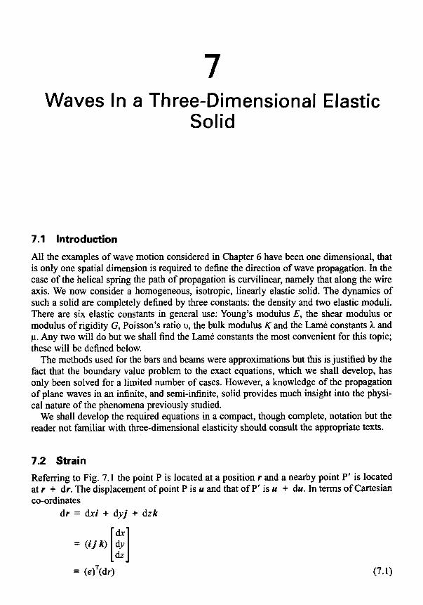
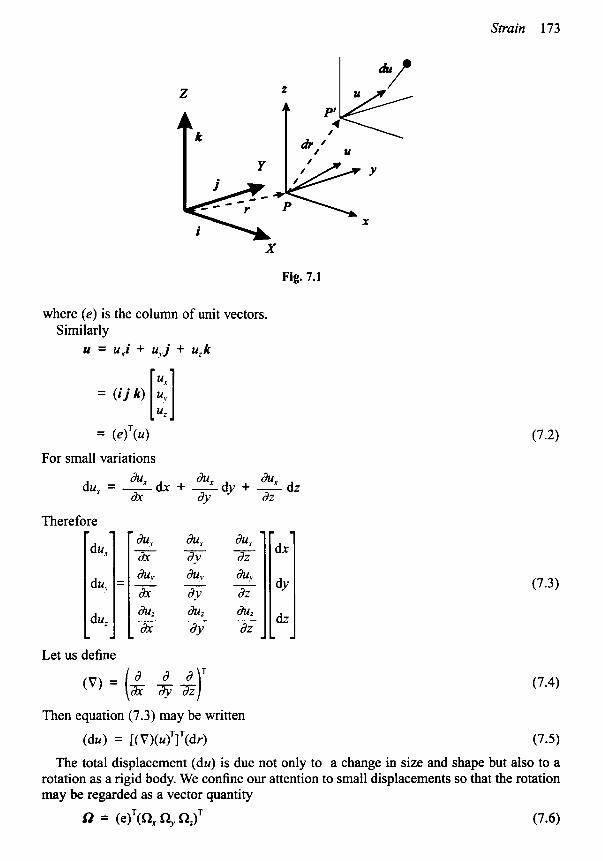
7 Waves In a Three-Dimensional Elastic Solid 7.1 Introduction All the examples of wave motion considered in Chapter 6 have been one dimensional, that is only one spatial dimension is required to define the direction of wave propagation. In the case of the helical spring the path of propagation is curvilinear, namely that along the wire axis. We now consider a homogeneous, isotropic, linearly elastic solid. The dynamics of such a solid are completely defined by three constants: the density and two elastic moduli. There are six elastic constants in general use: Young’s modulus E, the shear modulus or modulus of rigidity G, Poisson’s ratio u, the bulk modulus K and the Lame constants h and p. Any two will do but we shall find the Lame constants the most convenient for this topic; these will be defined below. The methods used for the bars and beams were approximations but this is justified by the fact that the boundary value problem to the exact equations, which we shall develop, has only been solved for a limited number of cases. However, a knowledge of the propagation of plane waves in an infinite, and semi-infinite, solid provides much insight into the physi- cal nature of the phenomena previously studied. We shall develop the required equations in a compact, though complete, notation but the reader not familiar with three-dimensional elasticity should consult the appropriate texts. 7.2 Strain Referring to Fig. 7.1 the point P is located at a position r and a nearby point P’ is located at r + dr. The displacement of point P is u and that of P’ is u + du. In terms of Cartesian co-ordinates dr = dxi + dyj + dzk
Transcript of Waves in Three Dimensional
7 Waves In a Three-Dimensional Elastic
Solid
7.1 Introduction
All the examples of wave motion considered in Chapter 6 have been one dimensional, that is only one spatial dimension is required to define the direction of wave propagation. In the case of the helical spring the path of propagation is curvilinear, namely that along the wire axis. We now consider a homogeneous, isotropic, linearly elastic solid. The dynamics of such a solid are completely defined by three constants: the density and two elastic moduli. There are six elastic constants in general use: Young’s modulus E, the shear modulus or modulus of rigidity G, Poisson’s ratio u, the bulk modulus K and the Lame constants h and p. Any two will do but we shall find the Lame constants the most convenient for this topic; these will be defined below.
The methods used for the bars and beams were approximations but this is justified by the fact that the boundary value problem to the exact equations, which we shall develop, has only been solved for a limited number of cases. However, a knowledge of the propagation of plane waves in an infinite, and semi-infinite, solid provides much insight into the physi- cal nature of the phenomena previously studied.
We shall develop the required equations in a compact, though complete, notation but the reader not familiar with three-dimensional elasticity should consult the appropriate texts.
7.2 Strain Referring to Fig. 7.1 the point P is located at a position r and a nearby point P’ is located at r + dr. The displacement of point P is u and that of P’ is u + du. In terms of Cartesian co-ordinates
d r = dxi + dyj + dzk
Strain 173
- du,
duv
du; m
- - -I - au, h x &
h v au, duy dy
6% d u z d u z &
- - aU, dy dz
. & dY dZ
& dY dz
- &
- (7.3) = - -
- - - - I -. -
- - - dub' a& d.7 dY dux a&
2 dz dx du, dub'
- -2 + - RX
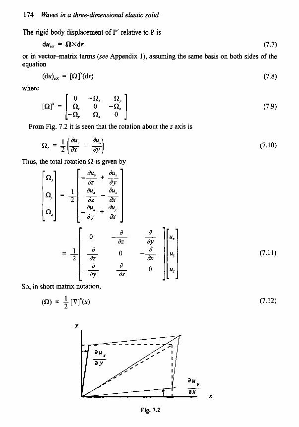
0, =r - - -
dY ax L
-- + 2 R* I -
Fig. 7.2
r - d
dZ dY d dx
0
0 a d
- d -- 0
-- =1- d 2 dz
- -- dY dx
m
UX
u,.
u2
(7.1 1)
- - -
Strain 175
or, in indicial notation,
Qi = 7 1 ( -Uj .k + Ukj ) (7.13)
The elastic displacement will be the total displacement less that due to rotation, so
(dulelastic = (dultaa~ - (du)rot (7.14)
From Appendix 1 or by direct multiplication we have that
(7.16)
(7.17)
The first term in the braces is given in equations (7.3) and (7.5) and the second term is its transpose, so half the sum of the two is a symmetric matrix which is the strain matrix [E]. Hence
where
Figure 7.2 shows the geometric definition of shear strain. In indicial notation
1 E.. = + . + u. .) !I 2 1 " J.1
(7.18)
(7.19)
(7.20)
(7.2 1)
Note that for i f j , tensile strain.
= $%, , that is half the conventional shear strain, whilst qi is the usual
176 Waves in a three-dimensional elastic solid
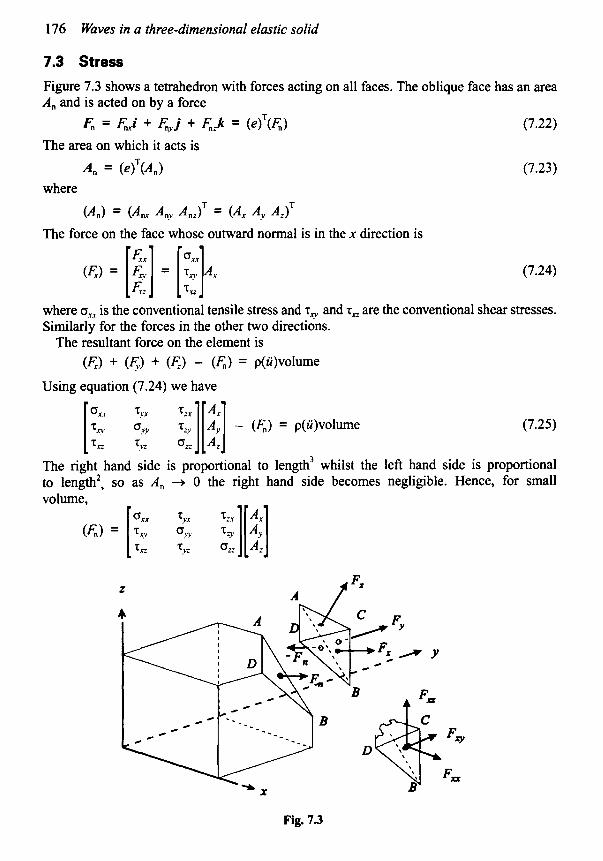
7.3 Stress Figure 7.3 shows a tetrahedron with forces acting on all faces. The oblique face has an area An and is acted on by a force
F, = ~ , i + 4,j + F,J = (e lT(4) (7.22) The area on which it acts is
An = (e)'(An) (7.23) where
(An) = (A, Any An;)T = ( ~ . r ~ . v ~ z ) ~
The force on the face whose outward normal is in the x direction is
(4) = [;] = [;jA,. (7.24)
where o,, is the conventional tensile stress and r? and r, are the conventional shear stresses. Similarly for the forces in the other two directions.
The resultant force on the element is (4) + (F,) + ( E ) - ( E ) = p(ii)volume
Using equation (7.24) we have
0x.r ~1.r '5, 4 [;I 2 ;][4 - (4) = p(Wolume (7.25)
The right hand side is proportional to length3 whilst the left hand side is proportional to length2, so as A , + 0 the right hand side becomes negligible. Hence, for small volume,
(6) = [:: !; ::I[::] r,, T,z 0,; 4
Fig. 7.3
Elastic constants 177
or (4) = [ol(An) (7.26)
where A, is a component of the area vector An and
o.r* ‘5w ‘52.r 0.n oyx 0 2 ,
‘5.r: ‘5,z 0;; 0x2 0, 0 2 ,
[ol = [ ‘5v “? T?] = [% 0.; %] (7.27)
is the stress matrix. The force vector is
F, = ( e ~ ~ [ o ~ ( ~ n ) = (e)T~o~(e)(e)T(~n) (7.28)
Note that (e)(e)T = [I] the unit matrix. The term (e)T[o](e) is the second-order stress tensor or dyadic. That is, it is the physical
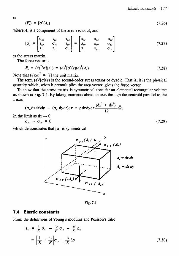
quantity which, when it premultiplies the area vector, gives the force vector. To show that the stress matrix is symmetrical consider an elemental rectangular volume
as shown in Fig. 7.4. By taking moments about an axis through the centroid parallel to the x axis
(dx’ + dy’) ii2 (ovdrdz)dy - (o,,dydZ)dx = pdxdydz
12 In the limit as dx + 0
OF - 0y.r = 0 (7.29)
which demonstrates that [o] is symmetrical.
Fig. 1.4
7.4 Elastic constants
From the definitions of Young’s modulus and Poisson’s ratio
- 1 u u E %r - r 0, - z o>v - - 0 2 2
(7.30) = [; + +]oxx + B3p u
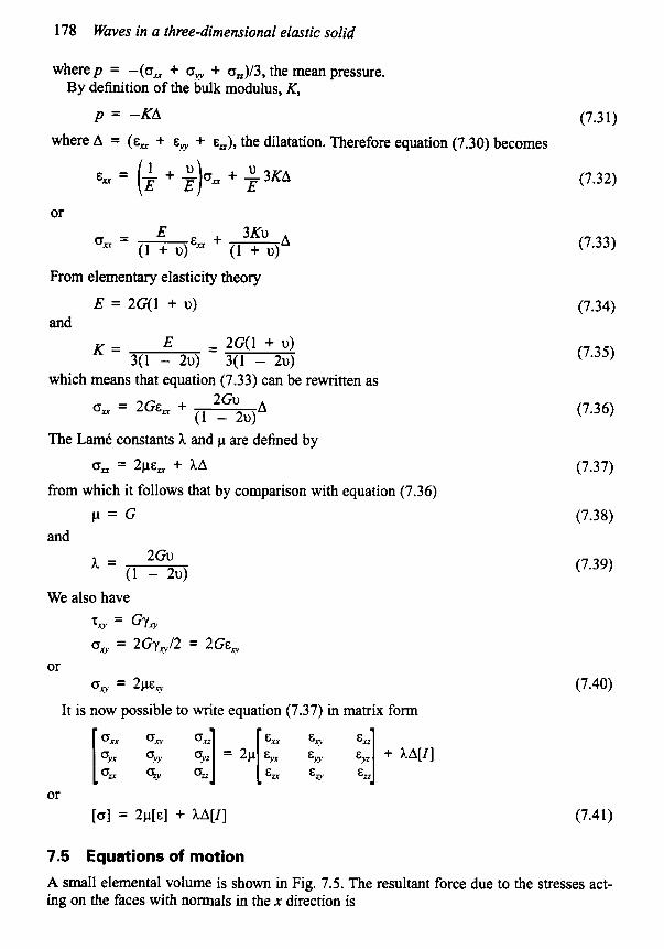
178 Waves in a three-dimensional elastic solid
where p = -(om + ow + o,)/3, the mean pressure. By definition of the bulk modulus, K,
p = -KA
where A = (E, + E . ~ + E=), the dilatation. Therefore equation (7.30) becomes
or
a,, = - E 3Ku A (1 + + - (1 + u)
From elementary elasticity theory
and E = 2G(1 + u)
E - - 2G(1 + u) K = 3(1 - 2 ~ ) 3(1 - 2 ~ )
which means that equation (7.33) can be rewritten as 2Gu A a,, = ~GE, , +
(1 - 2u) The Lame constants h and p are defined by
on = 2pX. + hA from which it follows that by comparison with equation (7.36)
and p = G
2Gu h = ( 1 - 2u)
We also have T q = GYP
ory = 2 P E q
oxy = 2Gyq/2 = ~ G E , or
It is now possible to write equation (7.37) in matrix form
or [o] = 2 p [ ~ ] + hA[Z]
7.5 Equations of motion
(7.3 1)
(7.32)
(7.33)
(7.34)
(7.35)
(7.36)
(7.37)
(7.38)
(7.39)
(7.40)
(7.41)
A small elemental volume is shown in Fig. 7.5. The resultant force due to the stresses act- ing on the faces with normals in the x direction is
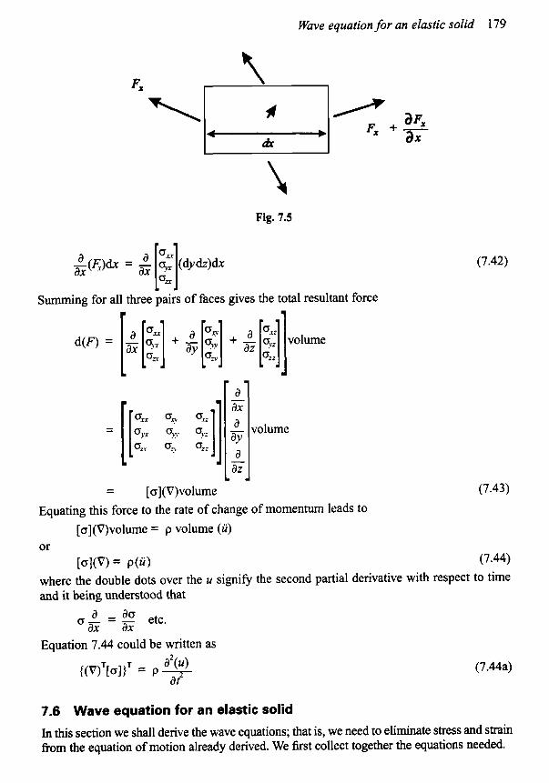
Wave equation for an elastic solid 179
- - a
ax
= [ 12 zz. 211 a aY a
az
-
a,, ozy 0 2 :
- L -
volume
180 Wmes in a three-dimensional elastic solid
Equation of motion rom = P(f4
kinematics
dilatation A = (V)'(U) = (u)'(V)
rotation (0) = [V]"(u) 1
and the elastic relationships [o] = 2p[&] + hA[Z]
Substituting equations (7.41) and (7.19) into (7.44) gives
P ((W)' + (V>(4T))(V) + hA[II(V) = P(fi)
cc (((v>T(w)'(v) + (V)'(V)(~)'(V))) + hA(V)'(V) = m'(a Now we premultiply by (V)' so that
and using (7.32)
p((A(V)'(V) + (V)T(V)A)) + hV% = pA
or
p (AV' + V'A) + hV2A = pA
Hence
(2p + h)V2A = pA
In full
ax ay2 az
which has the form of a classic wave equation in three dimensions. This time we premultiply equation (7.45) by [VI" so that
CI (([v1"(w7)' + [V1"(V)(u)T))(V) + A[VI"A(V) = P[VI"(ii)
p(2R)V' + (0) + (0) = p(2ii)
pV2(R) = p(ii)
Using equation (7.12) and noting that [V]"(V) = (0) we get
or
Expanding we get three equations of the form
(7.44)
(7.19)
(7.32)
(7.12)
(7.41)
(7.45)
(7.46)
(7.46a)
(7.47)
(7.47a)
Wave equation for an elastic solid 18 1
Again this is the form of a classic wave equation in three dimensions. The nature of the waves is best explored by the introduction of potential functions, one
scalar function of position and one vector function of position. The functions are assumed to be defined such that
(4 = (V)0 + [VI"(w) The dilatation is then
A = ( V ) T ( ~ ) = V2(0) + (V)T[V]x(~)
= V2(0) and twice the rotation
= [Vl"(U) = [VIX(V)0 + EvI"~l"(w)
(7.48)
(7.49)
= [v1"~1"~) (7.50) So we see that the dilatation is a function of the scalar function only and the rotation is a function of the vector function only.
The wave equations can be written in terms of the potential functions. Equation (7.46) becomes
(2p + h)v40 = p v 2 0 so
(2p + A)V20 = p0 Similarly equation (7.47) becomes
(7.5 1)
~v2~v1"~1"(w) = P [ v l x ~ ~ l x ( w )
[ v l x ~ ~ l x ~ v 2 ~ w ) = P[v1"~1"(\ii)
pV2(w) = P(W)
or
Therefore
Expanding equation (7.5 1) we get
A solution to this wave equation is 0 = f ( c t - s )
s = x + y + z
where s is a line with components x, y and z. It follows that since 2 2 2 2
a0 as ax - =f,, = fl
where I is the direction cosine between s and x. Similarly
(7.52)
(7.5 la)
a0 aY az 2 = fm and - = f n
Substitution into equation (7.51a) yields
182 Waves in a three-dimensional elastic solid
(2p + k)(l2 + m2 + n 2 r = p ( c 2 r
c = J [ ( 2 p + k ) /p ]
(u) = (V)'0
a0 ax
a0 u,, = - . aY
a0 u; = - az
As l2 + m2 + n2 = 1 the phase velocity of a wave travelling in the direction of s is
(7.53) The displacement, from equation (7.48), is
or
u, = -
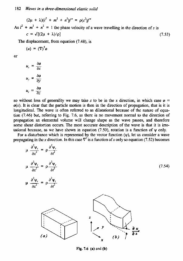
so without loss of generality we may take s to be in the x direction, in which case 0 = 0(x). It is clear that the particle motion is then in the direction of propagation, that is it is longitudinal. The wave is often referred to as dilatational because of the nature of equa- tion (7.46) but, refemng to Fig. 7.6, as there is no movement normal to the direction of propagation an elemental volume will change shape as the wave passes, and therefore some shear distortion occurs. The most accurate description of the wave is that it is irro- tational because, as we have shown in equation (7.50), rotation is a function of w only.
For a disturbance which is represented by the vector function (w), let us consider a wave propagating in the x direction. In this case V2 is a function ofx only so equation (7.52) becomes
2 a w, - a2w.r
pax ' -P2-
p a x 2 - - p 7
a2w* - a w z P 2 - P 7 ax
a2w, (7.54) 2 a w, -
2
Fig. 7.6 (a) and (b)
Wave equation for an elastic solid 183
The displacement is
or ux = -w?:z + WZ.."
u: = -wx,.V + w.v.x
u., = 0 u y - -w*.x
u z = W . r
uy = V.r.z - W , x
If (w) is a function of x only and (w) is constant in the yz plane then the displacement is
-
which shows that the displacement is wholly normal to the direction of propagation. It is possible to choose the orientation of the yz axes so that w, = 0 and the displacement is in the z direction only.
So, if awy ax
u; = -
the rotation (see equations (7.1 1 ) and (7.12))
i2r = Q, = 0 which shows that the rotation is about they axis. Figure 7.6(b) shows the deformation. From the figure it is clear that there is also shear deformation. As a result of this the wave is often called a shear wave but a more accurate description is equivoluminal because the dilatation is zero. The particle motion is transverse to the direction of propagation and is polarized because the direction of motion can be in any direction which is normal to the direction of propagation. The wave speed, from equation (7.52), is
J ( d P ) (7.55)
Summarizing the above results Correct name Irrotational Equivoluminal Common name Dilatational Shear In seismology Primary Secondary(Horizonta1 or Vertical),polarization Displacement Longitudinal Transverse Wave speed J [ ( 2 P + h)/Pl J ( d P ) Symbols cl, c d , cp c2, cs, CSH or CSV
184 Waves in a three-dimensional elastic solid
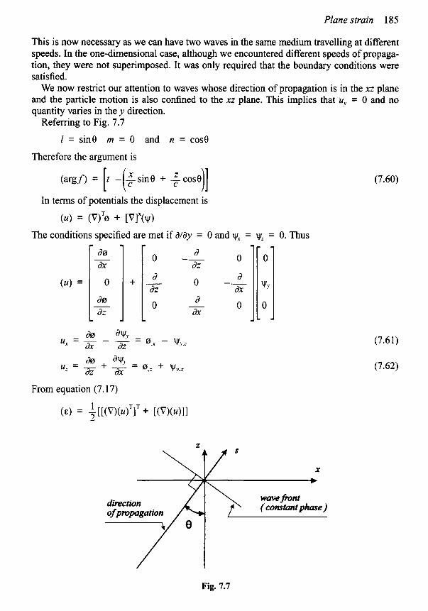
7.7 Plane strain In the previous section we studied a three-dimensional wave and found that two types of wave could be propagated, one with motion in the direction of travel and the other with motion normal to the direction of travel. Both types of wave arose as a solution to the three- dimensional wave equation in displacement u, rotation a, the scalar function 0 or the vec- tor function r. If the direction of propagation is parallel to a vector s = se, e being the unit vector, then we would expect a solution of the form used in the one-dimensional case to be applicable. So for any component of displacement we can write
u = f(cr - S)
for a wave travelling in the s direction. Now, choosing a suitable origin,
s = x i + y j + zk
and
e = li + mj + nk
where 1, m and n are the direction cosines of the vectors. So
s = e-s = lx + my + nz
and therefore
u = f(ct - s) = flct - (lx + my + nz)]
The argument offis,
(argf) = ct - (lx + my + nz)
(7.56)
(7.56a)
(we shall not use z in this chapter for the argument). If we choose to consider a sinusoidal wave of the form
= eJ(arp/)
then we introduce a quantity k, as before, where k has the dimension (l/length) and is the wavenumber. If we make k the magnitude of a vector K then the argument could be written
(argf) = ckr - ks = ckr - K.s
where
K = k,i + k,j + kzk
As before ck is identified as the circular frequency o, so (argf) = or - K-s
= or - (kx + k;r + kg)
(7.57)
(7.58)
If we wish to retain the use of an arbitrary functionfthen we need to modi@ the argument so that all wave functions have the same time component. This can be achieved by writing
c m (argf) = r - -x + -y + -z ( f c
(7.59)
I - - der ax
(u) = 0
- d 0 dZ
I -
Fig. 7.7
- _ _ - 0 0
a -- w, ax
- 0 0
d dz
0
d dx
-- 0
a dZ
0
+ -
- - I -
186 Waves in a three-dimensional elastic solid
Because the strain is planar we will need only the first and third rows and first and third columns. Thus
Hence the strain is
and the dilatation 2 A = V 0 = O.Lr + 0.=
From equation (7.41) the stress is
101 = 2Pkl + wll
(7.63)
(7.64)
which in two dimensions is
(7.65)
Note that although the strain is planar there will be a ov,, component of stress but this is not relevant in the problems to be discussed.
1 0,xx - '+$,z.r 0.K - +(y,:;r yvA 1 0 .xz - +(yy.:;- yv..rx) @.;z + y v , x z [GI = 2P
0 3 + 0,::
O I ..
+ O.=
7.8 Reflection at a plane surface
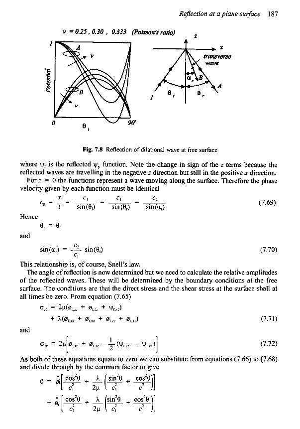
We shall now use the equations developed in the last section to study the reflection of a wave incident on a surface given by z = 0. First we consider a dilatational wave approaching the surface such that the direction of propagation makes an angle 0, with the normal to the surface, see Fig. 7.8. The potential hnction for this wave will be
z C
+ - cos(0,) (7.66)
We now assume that both a dilatational and a shear wave will be reflected; the functions will be z - -cos(@,) CI
(7.67)
(7.68)
Rejection at a plane su$ace 187
Fig. 7.8 Reflection of dilational wave at free surface
where wr is the reflected wy function. Note the change in sign of the z terms because the reflected waves are travelling in the negative z direction but still in the positive x direction.
For z = 0 the functions represent a wave moving along the surface. Therefore the phase velocity given by each function must be identical
(7.69) x - CI - CI - c2 --- --- - ‘P - i sin(ei) sin(0,) sin(%)
Hence
and e, = ei
(7.70) c2 CI
sin(a,) = - sin@,)
This relationship is, of course, Snell’s law. The angle of reflection is now determined but we need to calculate the relative amplitudes
of the reflected waves. These will be determined by the boundary conditions at the free surface. The conditions are that the direct stress and the shear stress at the surface shall at all times be zero. From equation (7.65)
- 0 2 2 - 2 P ( 0 i . z z + Or., + Wr,.rA
+ U0i.n + 0 r . n + 0i:z + 0r..u) (7.71)
and
(7.72)
As both of these equations equate to zero we can substitute from equations (7.66) to (7.68) and divide through by the common factor to give
1 Ox: - 2P 0i.c + 0.r: -- (vr .zz - Yr.ii)] - 1 2
II [cocs’e O = O i T + - ’’ [ c ; h A (9 + CO:~)]
2P CI
+ o r - + - A sin2e cos2e 2P (7 + 7-11 Cl
188 Waves in a three-dimensional elastic solid
and
where 8 = Oi = 8, and a = a,. The primes signify differentiation with respect to the argu- ment. Multiplying through by 2c: and taking 0, to be unity gives
From equations (7.38) and (7.39) h - 2u P (1 - 2u) - -
and from equations (7.53) and (7.55)
(7.73)
(7.74)
(7.75)
(Note that if u = 113 then Alp = 2 and c,/c2 = 2.) Given the angle of incidence equation (7.73) can be solved numerically for the relative
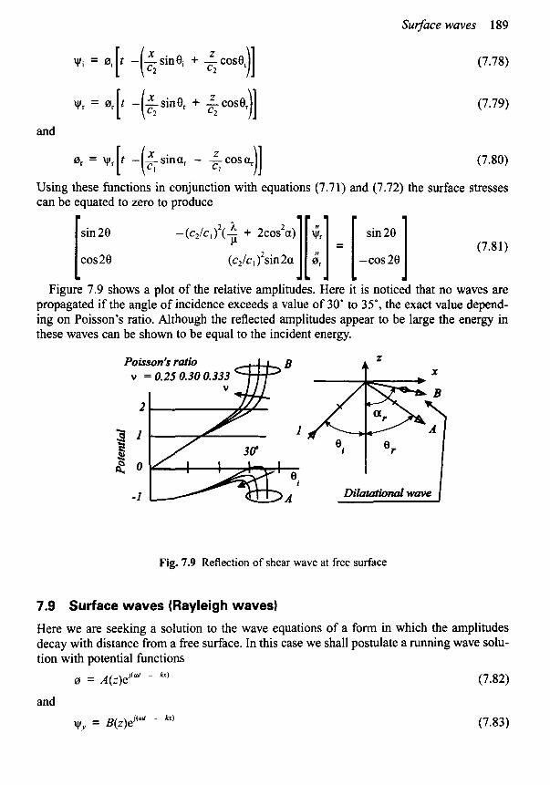
amplitudes. The results of such calculations are given on Fig. 7.8 for three values of Poisson’s ratio. Notice the sensitivity to Poisson’s ratio.
The above analysis gives the ratio of the second derivatives of the arbitrary potential func- tions, which will be the same as the ratios of the functions themselves. From equations (7.61) and (7.62) it is seen that for the dilatational waves
u, = 0, and uz = 0,:
so the displacement amplitude of a dilatational wave is
= 0’/CI
For the shear waves the displacement is
u, = -%,z and uz = yy,x
so the amplitude of a shear wave is
(7.76)
= w;/c, (7.77)
From equations (7.76) and (7.77) the relative amplitudes of the reflected waves may be found directly from the ratios of the potential functions.
For an incident shear wave the procedure is identical to that for the incident dilatational wave. Here the functions are
Suq4ace waves 189
(7.78)
(7.79)
)I vi = Oi[t -(;sinei + -cosei z
11 [ (.; c2
0, = \yr t - -sina, - -cosq)] Z 1 (;I CI
c2
z \yr = 0, t - x sine, + -case,
and
(7.80)
Using these functions in conjunction with equations (7.71) and (7.72) the surface stresses can be equated to zero to produce
sin 28 -(c2/c,f(+ + 2cos2a][ 4 = [ s in201 (7.81)
Figure 7.9 shows a plot of the relative amplitudes. Here it is noticed that no waves are propagated if the angle of incidence exceeds a value of 30" to 35"' the exact value depend- ing on Poisson's ratio. Although the reflected amplitudes appear to be large the energy in these waves can be shown to be equal to the incident energy.
C O S ~ B (c2/c, 12sin2a -cos20 1
Fig. 7.9 Reflection of shear wave at free surface
7.9 Surface waves (Rayleigh waves)
Here we are seeking a solution to the wave equations of a form in which the amplitudes decay with distance from a free surface. In this case we shall postulate a running wave solu- tion with potential functions
(7.82) 0 = A(Z)eJ'& - kr)
and
w,, = B(z)e"& - ICr) (7.83)
190 Waves in a three-dimensional elastic solid
which is compatible with particle movement in the xz plane, as in the previous section. Also we have the same boundary condition of zero stress at the free surface.
The wave equation (7.51) can be written 2
c,(0,, + 0 Z: ) = 0
Substituting from equation (7.82) and dividing through by the common factor gives
or
Let
so that
d 5 - &A = 0
(7.84)
(7.85)
(7.86)
The general solution to this equation is
where a and b are arbitrary constants.
and thus a =A,. Hence
A = ae-Pli + bgi' (7.87)
We require A to tend to zero as z tends to infinity and therefore b = 0 and at z = 0, A = A o
A(z) = AOePli (7.88) The wave equation (7.52) can be written as
cf(y.v,.r.r + ~ y , z z ) = 8. so substituting equation (7.83) yields
where B(z) = BOe-P2i (7.89)
(7.90)
(7.9 1)
(7.92)
Surface waves 191
Thusatz = 0
0 = 2p(p:A0 - jkp2B0) + h(-k20 + p:Bo)
0 = 2p -jkp,A, -7(p2 1 2 + k2)Bo] I or
From equations (7.38) and (7.39) L= 2u
CI 1 - 2 u
and
(7.93)
Let
(c,/c,) = R
Thus h/p = R - 2
Dividing all terms in equation (7.93) by pk2 gives
(7.94)
-j2J[1 - ~c~)~ ’1 [^ .1 = [:I (7.95) (R[1 - (dc,),] - (R - 2))
- j 2 ~ [ 1 - (c/cI)’] -[1 - (c/c2)’ + 13 Bo
For a non-trivial solution the determinant of the square matrix must be zero. Thus
-[2 - (c/cJ2I2 + W([1 - ( c / ~ ~ ) ~ / R ] [ l - (c/c2f]} = 0
A little more algebra leads to the following cubic in (c/c2f
(er - 8(er + (24 --$)(e/ + (g - 16) = 0 (7.96)
where
(7.97) 1 - u 1 - 2u
R = (c1/c2), =
It is well known that for a positive Poisson’s ratio the value cannot exceed 0.5. Analysis of the cubic shows that there is always one real root with c 0.263 there are three real roots but the upper two are for wave speeds greater than c, which are not admissible. The speed of the Rayleigh wave does not depend on frequency but only on the elastic constants.
c2. For u
From the first equation of (7.95) the ratio of the amplitudes is
(7.98)
192 Waves in a three-dimensional elastic solid
(7.99) The computed values of wave speed and relative amplitudes of the potentials are given in
For ease of reference let Bo/Ao = -ip.
the following table:
u 0.250 0.300 0.333 CIC, 0.919 0.927 0.933 BOIA 0 -j 1.47 -j 1.52 -j 1.56
From equations (7.61) and (7.62) we have
U r = 0.1- - wy;
and
uz = 0,: + w,..,
u, = A,e-'~~-jkd'"' - A) - ~,e-*2'-~2 d'"y - /a)
Substituting from equations 7.91 and 7.92
u; = A,e-"l'- - Pe'(& - kr) + B0e-'zz-jk d" - kr)
Atx = 0,z = Oweget
u, = (-jkA, + p2BO)eJo'
uL = (-plAo - jkB0)eJd (7.100)
(7.101) Using equation (7.99) the ratio of the displacements may be written as
u: - u.r
-jk(l + P J [ ~ - (c/c~)~I) -k(J[l - (c/c~)~(c~/c,)~] + P}
For u = 0.3 we have that c/c2 = 0.927 and p = 1.52. Thus
_ - (7.102)
(7.103)
This means that the amplitude of the displacement in the z direction is 1.52 times that in the x direction and is leading by 90'. That is, the motion is elliptical with the major axis verti- cal and the particle motion anti-clockwise.
The Rayleigh waves are similar to deep-water gravity waves except that the speed does not depend on wavelength. When dealing with high-frequency waves in a bar the Rayleigh wave is often the form of propagation, the motion being concentrated in the region near the surface. The exact solution for waves in an infinite cylindrical bar was developed by Pochammer and Chree and here the Rayleigh wave was the form for high-frequency axial and bending waves.
7.10 Conclusion
In these last two chapters we have attempted to bring out the most important physical aspects of wave propagation in elastic solids. Many of the ideas are new when compared with rigid body mechanics and to normal mode vibration theory. Wave methods are most useful for short-duration phenomena such as impact. The time scale is judged by compar-
Conclusion 193
ing the impact time with the time taken for a disturbance to be reflected back from a boundary. Large-scale events like earthquakes require wave study and so do small-scale events where the wave speed is relatively low, as in problems involving springs.
The three-dimensional waves have been described using Cartesian co-ordinates but many interesting problems are best solved using cylindrical or spherical co-ordinates. The funda- mental equations have been developed using the vector operator
= (elT(V) = (VlT(e> The operations on a typical scalar 0 and a typical vector y can be summarized.
The matrix form (V)0 has its vector counterpart (C?)~(V)O = VO = gradient 0
Similarly (V)T(y.r) = (V)T(e)*(e)T(W) is the scalar
Also [V]"(w) = [V]"(e)-(e)T(~) has its vector form
V y = divergence y
( ( e ) T [ ~ ~ x ( e ) } . ( ( e ) T ( ~ ) } = V X ~ = curl(or rot) y
Because all the equations derived in this chapter assume a common basis for the vectors (i.e. i,j and k) the following identities can be made
(V)0 = grad0 ( V T ( W ) diVW
[VI"(W) = curly The expressions for div, grad and curl in cylindrical and spherical co-ordinates are given in Appendix 3. Also included are the relevant expressions for stress and strain.