A&A 446, 1191–1204 (2006)DOI: 10.1051/0004-6361:20053246c© ESO 2006

Astronomy&

Astrophysics

Wavelets, ridgelets and curvelets on the sphere�

J.-L. Starck1,2, Y. Moudden1, P. Abrial1, and M. Nguyen3

1 DAPNIA/SEDI-SAP, Service d’Astrophysique, CEA-Saclay, 91191 Gif-sur-Yvette Cedex, Francee-mail: jstarck@cea.fr

2 Department of Statistics, Sequoia Hall, 390 Serra Mall, Stanford University, Stanford, CA 94305, USA3 Laboratoire Traitement de l’Image et du Signal, CNRS UMR 8051/ENSEA/Université de Cergy-Pontoise,

ENSEA, 6 avenue du ponceau, 95014 Cergy, France

Received 15 April 2005 / Accepted 8 September 2005

ABSTRACT

We present in this paper new multiscale transforms on the sphere, namely the isotropic undecimated wavelet transform, the pyramidal wavelettransform, the ridgelet transform and the curvelet transform. All of these transforms can be inverted i.e. we can exactly reconstruct the originaldata from its coefficients in either representation. Several applications are described. We show how these transforms can be used in denoisingand especially in a Combined Filtering Method, which uses both the wavelet and the curvelet transforms, thus benefiting from the advantagesof both transforms. An application to component separation from multichannel data mapped to the sphere is also described in which we takeadvantage of moving to a wavelet representation.

Key words. cosmic microwave background – methods: data analysis – methods: statistical

1. Introduction

Wavelets in astronomy

Wavelets are very popular tools in astronomy (Starck &Murtagh 2002) which have led to very impressive results indenoising and detection applications. For instance, both theChandra and the XMM data centers use wavelets for the de-tection of extended sources in X-ray images. For denoising anddeconvolution, wavelets have also demonstrated how power-ful they are for discriminating signal from noise (Starck et al.2002b). In cosmology, wavelets have been used in many stud-ies such as for analyzing the spatial distribution of galaxies(Slezak et al. 1993; Escalera & MacGillivray 1995; Starcket al. 2005a; Martinez et al. 2005), determining the topology ofthe universe (Rocha et al. 2004), detecting non-Gaussianity inthe CMB maps (Aghanim & Forni 1999; Barreiro et al. 2001;Vielva et al. 2004; Starck et al. 2004), reconstructing the pri-mordial power spectrum (Mukherjee & Wang 2003), measur-ing the galaxy power spectrum (Fang & Feng 2000) or re-constructing weak lensing mass maps (Starck et al. 2005b).It has also been shown that noise is a problem of major con-cern for N-body simulations of structure formation in the earlyUniverse and that using wavelets to remove noise from N-bodysimulations is equivalent to simulations with two orders ofmagnitude more particles (Romeo et al. 2003, 2004).

� Appendices A and B are only available in electronic form athttp://www.edpsciences.org

The most popular wavelet algorithm in astrophysical appli-cations is the so-called “à trous algorithm”. It is an isotropicundecimated wavelet transform in which the scaling functionused is a Box-Spline of order three. The isotropy of the waveletfunction makes this decomposition optimal for the detection ofisotropic objects. The non decimation makes the decomposi-tion redundant (the number of coefficients in the decomposi-tion is equal to the number of samples in the data multipliedby the number of scales) and allows us to avoid Gibbs aliasingafter reconstruction in image restoration applications, as gen-erally occurs with orthogonal or bi-orthogonal wavelet trans-forms. The choice of a B3-spline is motivated by the fact thatwe want an analyzing function close to a Gaussian, but veri-fying the dilation equation, which is required in order to havea fast transformation. One last property of this algorithm is toprovide a very straightforward reconstruction. Indeed, the sumof all the wavelet scales and of the coarsest resolution imagereproduces exactly the original image.

When analyzing data that contains anisotropic features,wavelets are no longer optimal and this has motivated thedevelopment of new multiscale decompositions such as theridgelet and the curvelet transforms (Donoho & Duncan 2000;Starck et al. 2002a). In Starck et al. (Starck et al. 2004), ithas been shown that the curvelet transform could be usefulfor the detection and the discrimination of non Gaussianity inCMB data. In this area, further insight will come from the anal-ysis of full-sky data mapped to the sphere thus requiring thedevelopment of a curvelet transform on the sphere.

Article published by EDP Sciences and available at http://www.edpsciences.org/aa or http://dx.doi.org/10.1051/0004-6361:20053246

1192 J.-L. Starck et al.: Wavelets, ridgelets and curvelets on the sphere

Wavelets on the sphere

Several wavelet transforms on the sphere have been proposedin recent years. Schröder & Sweldens (1995) have developedan orthogonal wavelet transform on the sphere based on theHaar wavelet function. Its interest is however relatively lim-ited because of the poor properties of the Haar function andthe problems inherent to the orthogonal decomposition. Manypapers describe new continuous wavelet transforms (Antoine1999; Tenorio et al. 1999; Cayón et al. 2001; Holschneider1996) and the recent detection of non-Gaussianity in CMB wasobtained by Vielva et al. (Vielva et al. 2004) using the con-tinuous Mexican Hat wavelet transform (Cayón et al. 2001).These works have been extended to directional wavelet trans-forms (Antoine et al. 2002; McEwen et al. 2004; Wiaux et al.2005). All these new continuous wavelet decompositions areinteresting for data analysis, but cannot be used for restora-tion purposes because of the lack of an inverse transform.Only the algorithm proposed by Freeden and Maier (Freeden& Windheuser 1997; Freeden & Schneider 1998), based on theSpherical Harmonic Decomposition, has an inverse transform.

The goal of this paper is to extend existing 2D multiscaledecompositions, namely the ridgelet transform, the curvelettransform and the isotropic wavelet transform, which work onflat images to multiscale methods on the sphere. In Sect. 2, wepresent a new isotropic wavelet transform on the sphere whichhas similar properties to the à trous algorithm and thereforeshould be very useful for data denoising and deconvolution.This algorithm is directly derived from the FFT-based wavelettransform proposed in Starck et al. (1994) for aperture synthe-sis image restoration, and is relatively close to the Freeden &Maier (Freeden & Schneider 1998) method, except that it fea-tures the same straightforward reconstruction as the à trous al-gorithm (i.e. the sum of the scales reproduces the original data).This new wavelet transform also can be easily extended to apyramidal wavelet transform, hence with reduced redundancy,a possibility which may be very important for larger data setssuch as expected from the future Planck-Surveyor experiment.In Sect. 3, we show how this new decomposition can be used toderive a curvelet transform on the sphere. Section 4 describeshow these new transforms can be used in denoising applica-tions and introduces the Combined Filtering Method, whichallows us to filter data on the sphere using both the Waveletand the Curvelet transforms. In Sect. 5, we show that the inde-pendent component analysis method wSMICA (Moudden et al.2005), which was designed for 2D data, can be extended to dataon the sphere.

2. Wavelet transform on the sphere

2.1. Isotropic undecimated wavelet transformon the sphere (UWTS)

There are clearly many different possible implementations of awavelet transform on the sphere and their performance dependson the application. We describe here an undecimated isotropictransform which has many properties in common with theà trous algorithm, and is therefore a good candidate for restora-tion applications. Its isotropy is a favorable property when

analyzing a statistically isotropic Gaussian field such as theCMB or data sets such as maps of galaxy clusters, which con-tain only isotropic features (Starck et al. 1998). Our isotropictransform is obtained using a scaling function φlc (ϑ, ϕ) withcut-off frequency lc and azimuthal symmetry, meaning that φlcdoes not depend on the azimuth ϕ. Hence the spherical har-monic coefficients φlc (l,m) of φlc vanish when m � 0 so that:

φlc(ϑ, ϕ) = φlc (ϑ) =l=lc∑l=0

φlc (l, 0)Yl,0(ϑ, ϕ) (1)

where the Yl,m are the spherical harmonic basis functions. Then,convolving a map f (ϑ, ϕ) with φlc is greatly simplified and thespherical harmonic coefficients c0(l,m) of the resulting mapc0(ϑ, ϕ) are readily given by (Bogdanova et al. 2005):

c0(l,m) = φlc ∗ f (l,m) =

√4π

2l + 1φlc (l, 0) f (l,m) (2)

where ∗ stands for convolution.

Multiresolution decompostion

A sequence of smoother approximations of f on a dyadic res-olution scale can be obtained using the scaling function φlc asfollows

c0 = φlc ∗ f

c1 = φ2−1lc ∗ f

. . .

c j = φ2− j lc ∗ f (3)

where φ2− j lc is a rescaled version of φlc with cut-off fre-quency 2− jlc. The above multi-resolution sequence can alsobe obtained recursively. Define a low pass filter h j for eachscale j by

H j(l,m) =

√4π

2l + 1h j(l,m)

=

⎧⎪⎪⎪⎪⎨⎪⎪⎪⎪⎩φ lc

2 j+1(l,m)

φ lc2 j

(l,m)if l < lc

2 j+1 and m = 0

0 otherwise.

(4)

It is then easily shown that c j+1 derives from c j by convolutionwith h j: c j+1 = c j ∗ h j.

The wavelet coefficients

Given an axisymmetric wavelet function ψlc , we can derive inthe same way a high pass filter g j on each scale j:

G j(l,m) =

√4π

2l + 1g j(l,m)

=

⎧⎪⎪⎪⎪⎪⎪⎪⎨⎪⎪⎪⎪⎪⎪⎪⎩

ψ lc2 j+1

(l,m)

φ lc2 j

(l,m)if l < lc

2 j+1 and m = 0

1 if l ≥ lc2 j+1 and m = 0

0 otherwise.

(5)

J.-L. Starck et al.: Wavelets, ridgelets and curvelets on the sphere 1193

Fig. 1. On the left, the scaling function φ and, on the right, the wavelet function ψ.

Using these, the wavelet coefficients w j+1 at scale j + 1 areobtained from the previous resolution by a simple convolution:w j+1 = c j ∗ g j.

Just as with the à trous algorithm, the wavelet coefficientscan be defined as the difference between two consecutive reso-lutions, w j+1(ϑ, ϕ) = c j(ϑ, ϕ) − c j+1(ϑ, ϕ), which in fact corre-sponds to making the following specific choice for the waveletfunction ψlc :

ψ lc2 j

(l,m) = φ lc2 j−1

(l,m) − φ lc2 j

(l,m). (6)

The high pass filters g j defined above are, in this particularcase, expressed as:

G j(l,m) =

√4π

2l + 1g j(l,m)

= 1 −√

4π2l + 1

h j(l,m) = 1 − H j(l,m). (7)

Obviously, other wavelet functions could be used as well.

Choice of the scaling function

Any function with a cut-off frequency is a possible candidate.We retained here a B-spline function of order 3. It is very closeto a Gaussian function and converges rapidly to 0:

φlc (l,m = 0) =32

B3

(2llc

)(8)

where B(x) = 112 (| x − 2 |3 − 4| x − 1 |3 + 6| x |3 − 4| x + 1 |3 +

| x + 2 |3).In Fig. 1 the chosen scaling function derived from a

B-spline of degree 3, and its resulting wavelet function, areplotted in frequency space.

The numerical algorithm for the undecimated wavelettransform on the sphere is:

1. Compute the B3-spline scaling function and derive ψ, h andg numerically.

2. Compute the corresponding Spherical Harmonics of imagec0. We get c0.

3. Set j to 0. Iterate:4. Multiply c j by H j. We get the array c j+1.

Its inverse Spherical Harmonics Transform gives the im-age at scale j + 1.

5. Multiply c j by G j. We get the complex array w j+1.The inverse Spherical Harmonics transform of w j+1 givesthe wavelet coefficients w j+1 at scale j + 1.

6. j = j + 1 and if j ≤ J, return to Step 4.7. The set {w1, w2, . . . , wJ, cJ} describes the wavelet transform

on the sphere of c0.

Reconstruction

If the wavelet is the difference between two resolutions, Step 5in the above UWTS algorithm can be replaced by the follow-ing simple subtraction w j+1 = c j − c j+1. In this case, the re-construction of an image from its wavelet coefficients W =

{w1, . . . , wJ , cJ} is straightforward:

c0(θ, φ) = cJ(θ, φ) +J∑

j=1

w j(θ, φ). (9)

This is the same reconstruction formula as in the à trous al-gorithm: the simple sum of all scales reproduces the originaldata. However, since the present decomposition is redundant,the procedure for reconstructing an image from its coefficientsis not unique and this can profitably be used to impose addi-tional constraints on the synthesis functions (e.g. smoothness,positivity) used in the reconstruction. Here for instance, usingthe relations:

c j+1(l,m) = H j(l,m)c j(l,m)

w j+1(l,m) = G j(l,m)c j(l,m) (10)

a least squares estimate of c j from c j+1 and w j+1 gives:

c j = c j+1H j + w j+1

G j (11)

where the conjugate filters H j and G j have the expression:

H j =

√4π

2l + 1ˆhj = H∗j/(| H j |2 + | G j |2) (12)

G j =

√4π

2l + 1ˆg j = G∗j/(| H j |2 + | G j |2) (13)

1194 J.-L. Starck et al.: Wavelets, ridgelets and curvelets on the sphere

Fig. 2. On the left, the filter ˆh, and on the right the filter ˆg.

and the reconstruction algorithm is:

1. Compute the B3-spline scaling function and derive ψ, h, g,ˆh, ˆg numerically.

2. Compute the corresponding Spherical Harmonics of the im-age at the low resolution cJ . We get cJ.

3. Set j to J − 1. Iterate:4. Compute the Spherical Harmonics transform of the

wavelet coefficients w j+1 at scale j + 1. We get w j+1.

5. Multiply c j+1 by H j.

6. Multiply w j+1 by G j.7. Add the results of steps 6 and 7. We get c j.8. j = j − 1 and if j ≥ 0, return to Step 4.

9. Compute The inverse Spherical Harmonic transform of c0.

The synthesis low pass and high pass filters ˆh and ˆg are plottedin Fig. 2.

Figure 3 shows the WMAP data (top left) and its undeci-mated wavelet decomposition on the sphere using five resolu-tion levels. Figures 3 middle left, middle right and bottom leftshow respectively the four wavelet scales. Figure 3 bottom rightshows the last smoothed array. Figure 4 shows the backprojec-tion of a wavelet coefficient at different scales and positions.

2.2. Isotropic pyramidal wavelet transformon the sphere (PWTS)

In the previous algorithm, no downsampling is performed andeach scale of the wavelet decomposition has the same numberof pixels as the original data set. Therefore, the number of pix-els in the decomposition is equal to the number of pixels in thedata multiplied by the number of scales. For applications suchas PLANCK data restoration, we may prefer to introduce somedecimation in the decomposition so as to reduce the requiredmemory size and the computation time. This can be done eas-ily by using a specific property of the chosen scaling function.Indeed, since we are considering here a scaling function withan initial cut-off lc in spherical harmonic multipole number l,

and since the actual cut-off is reduced by a factor of two at eachstep, the number of significant spherical harmonic coefficientsis then reduced by a factor of four after each convolution withthe low pass filter h. Therefore, we need fewer pixels in thedirect space when we compute the inverse spherical harmonictransform. Using the Healpix pixelization scheme (Górski et al.2002), this can be done easily by dividing by 2 the nside param-eter when resorting to the inverse spherical harmonic transformroutine.

Figure 5 shows WMAP data (top left) and its pyramidalwavelet transform using five scales. As the scale number in-creases (i.e. the resolution decreases), the pixel size becomeslarger. Figures 5 top right, middle left, middle right and bottomleft show respectively the four wavelet scales. Figure 5 bottomright shows the last smoothed array.

3. Curvelet transform on the sphere (CTS)

3.1. Introduction

The 2D curvelet transform, proposed in Donoho & Duncan(2000), Starck et al. (2002a, 2003a) enables the directionalanalysis of an image in different scales. The fundamental prop-erty of the curvelet transform is to analyze the data with func-tions of length of about 2− j/2 for the jth sub-band [2 j, 2 j+1]of the two dimensional wavelet transform. Following the im-plementation described in Starck et al. (2002a) and Starcket al. (2003a), the data first undergoes an isotropic undecimatedwavelet transform (i.e. à trous algorithm). Each scale j is thendecomposed into smoothly overlapping blocks of side-lengthB j pixels in such a way that the overlap between two verti-cally adjacent blocks is a rectangular array of size B j × B j/2.Finally, the ridgelet transform (Candès & Donoho 1999) isapplied on each individual block which amounts to applyinga 1-dimensional wavelet transform to the slices of its Radontransform. More details on the implementation of the digitalcurvelet transform can be found in Starck et al. (2002a, 2003a).It has been shown that the curvelet transform could be veryuseful for the detection and the discrimination of sources of

J.-L. Starck et al.: Wavelets, ridgelets and curvelets on the sphere 1195

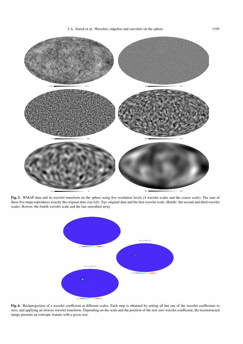
Fig. 3. WMAP data and its wavelet transform on the sphere using five resolution levels (4 wavelet scales and the coarse scale). The sum ofthese five maps reproduces exactly the original data (top left). Top: original data and the first wavelet scale. Middle: the second and third waveletscales. Bottom: the fourth wavelet scale and the last smoothed array.

Fig. 4. Backprojection of a wavelet coefficient at different scales. Each map is obtained by setting all but one of the wavelet coefficients tozero, and applying an inverse wavelet transform. Depending on the scale and the position of the non zero wavelet coefficient, the reconstructedimage presents an isotropic feature with a given size.

1196 J.-L. Starck et al.: Wavelets, ridgelets and curvelets on the sphere

Fig. 5. WMAP data (top left) and its pyramidal wavelet transform on the sphere using five resolution levels (4 wavelet scales and the coarsescale). The original map can be reconstructed exactly from the pyramidal wavelet coefficients. Top: original data and the first wavelet scale.Middle: the second and third wavelet scales. Bottom: the fourth wavelet scale and the last smoothed array. The number of pixels is divided byfour at each resolution level, which can be helpful when the data set is large.

non-Gaussianity in CMB (Starck et al. 2003b). The curvelettransform is also redundant, with a redundancy factor of 16J+1whenever J scales are employed. Its complexity scales like thatof the ridgelet transform that is as O(n2 log2 n). This methodis best for the detection of anisotropic structures and smoothcurves and edges of different lengths.

3.2. Curvelets on the sphere

The curvelet transform on the sphere (CTS) can be similar tothe 2D digital curvelet transform, but replacing the à trous al-gorithm by the isotropic wavelet transform on the sphere previ-ously described. The CTS algorithm consists of the followingthree steps:

– Isotropic wavelet transform on the sphere.– Partitioning. Each scale is decomposed into blocks of an

appropriate scale (of side-length ∼2−s), using the Healpixpixelization.

– Ridgelet analysis. Each square is analyzed via the discreteridgelet transform.

Partitioning using the Healpix representation

The Healpix representation is a curvilinear partition of thesphere into quadrilateral pixels of exactly equal area but withvarying shape. The base resolution divides the sphere into12 quadrilateral faces of equal area placed on three ringsaround the poles and equator. Each face is subsequently dividedinto nside2 pixels following a hierarchical quadrilateral treestructure. The geometry of the Healpix sampling grid makesit easy to partition a spherical map into blocks of a specifiedsize 2n. We first extract the twelve base-resolution faces, andeach face is then decomposed into overlapping blocks as in the2D digital curvelet transform. With this scheme however, thereis no overlapping between blocks belonging to different base-resolution faces. This may result in blocking effects for exam-ple in denoising experiments via non linear filtering. A simple

J.-L. Starck et al.: Wavelets, ridgelets and curvelets on the sphere 1197

Fig. 6. Flowgraph of the ridgelet transform on the sphere.

way around this difficulty is to work with various rotations ofthe data with respect to the sampling grid.

Ridgelet transform

Once the partitioning is performed, the standard 2D ridgelettransform described in Starck et al. (2003a) is applied in eachindividual block:

1. Compute the 2D Fourier transform.2. Extract lines going through the origin in the frequency

plane.3. Compute the 1D inverse Fourier transform of each line.

This achieves the Radon transform of the current block.4. Compute the 1D wavelet transform of the lines of the

Radon transform.

The first three steps correspond to a Radon transform methodcalled the linogram. Other implementations of the Radon trans-form, such as the Slant Stack Radon Transform (Donoho &Flesia 2002), can be used as well, as long as they offer an exactreconstruction.

Figure 6 shows the flowgraph of the ridgelet transform onthe sphere and Fig. 7 shows the backprojection of a ridgeletcoefficient at different scales and orientations.

3.3. Algorithm

The curvelet transform algorithm on the sphere is as follows:

1. Apply the isotropic wavelet transform on the sphere withJ scales.

2. Set the block size B1 = Bmin.3. For j = 1, . . . , J do,

– partition the subband w j with a block size B j and applythe digital ridgelet transform to each block;

Fig. 7. Backprojection of a ridgelet coefficient at different scales andorientations. Each map is obtained by setting all but one of theridgelet coefficients to zero, and applying an inverse ridgelet trans-form. Depending on the scale and the position of the non zero ridgeletcoefficient, the reconstructed image presents a feature with a givenwidth and a given orientation.

– if j modulo 2 = 1 then B j+1 = 2B j;– else B j+1 = B j.

The sidelength of the localizing windows is doubled at ev-ery other dyadic subband, hence maintaining the fundamentalproperty of the curvelet transform which says that elementsof length about 2− j/2 serve for the analysis and synthesis ofthe j-th subband [2 j, 2 j+1]. We used the default value Bmin =

16 pixels in our implementation. Figure 8 gives an overviewof the organization of the algorithm. Figure 9 shows thebackprojection of curvelet coefficients at different scales andorientations.

1198 J.-L. Starck et al.: Wavelets, ridgelets and curvelets on the sphere

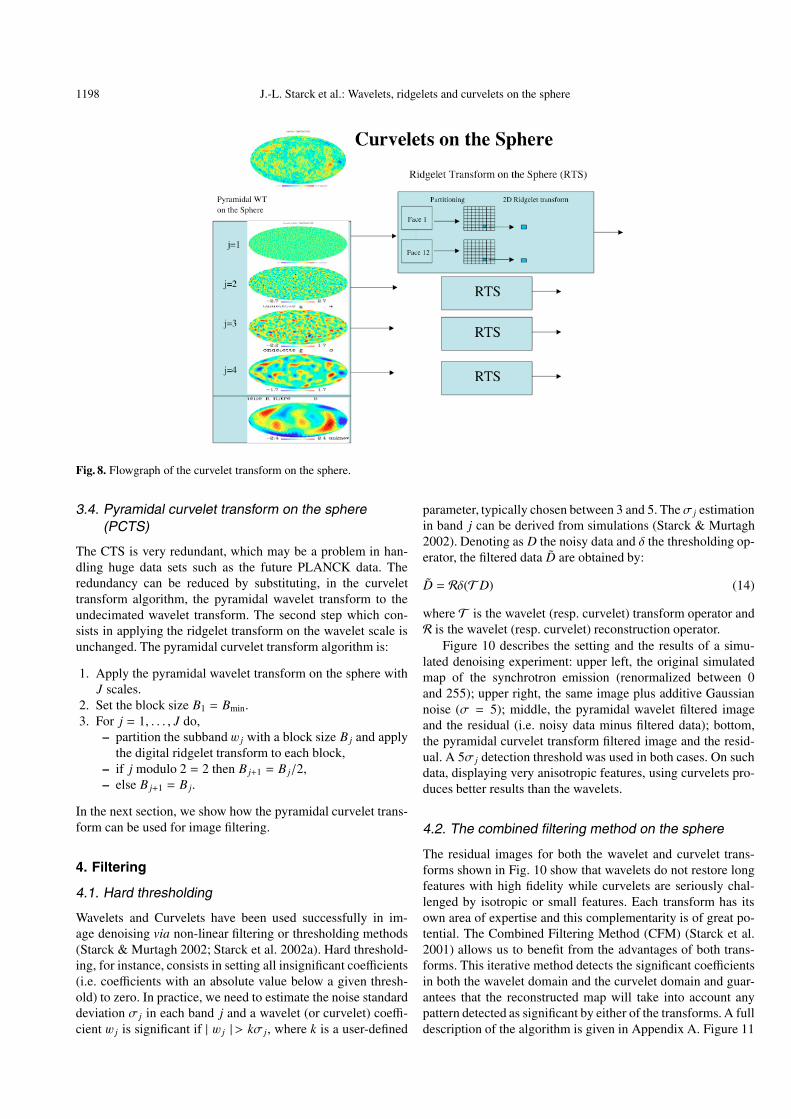
Fig. 8. Flowgraph of the curvelet transform on the sphere.

3.4. Pyramidal curvelet transform on the sphere(PCTS)

The CTS is very redundant, which may be a problem in han-dling huge data sets such as the future PLANCK data. Theredundancy can be reduced by substituting, in the curvelettransform algorithm, the pyramidal wavelet transform to theundecimated wavelet transform. The second step which con-sists in applying the ridgelet transform on the wavelet scale isunchanged. The pyramidal curvelet transform algorithm is:

1. Apply the pyramidal wavelet transform on the sphere withJ scales.

2. Set the block size B1 = Bmin.3. For j = 1, . . . , J do,

– partition the subband w j with a block size B j and applythe digital ridgelet transform to each block,

– if j modulo 2 = 2 then B j+1 = B j/2,– else B j+1 = B j.

In the next section, we show how the pyramidal curvelet trans-form can be used for image filtering.

4. Filtering

4.1. Hard thresholding

Wavelets and Curvelets have been used successfully in im-age denoising via non-linear filtering or thresholding methods(Starck & Murtagh 2002; Starck et al. 2002a). Hard threshold-ing, for instance, consists in setting all insignificant coefficients(i.e. coefficients with an absolute value below a given thresh-old) to zero. In practice, we need to estimate the noise standarddeviation σ j in each band j and a wavelet (or curvelet) coeffi-cient w j is significant if | w j |> kσ j, where k is a user-defined

parameter, typically chosen between 3 and 5. Theσ j estimationin band j can be derived from simulations (Starck & Murtagh2002). Denoting as D the noisy data and δ the thresholding op-erator, the filtered data D are obtained by:

D = Rδ(TD) (14)

where T is the wavelet (resp. curvelet) transform operator andR is the wavelet (resp. curvelet) reconstruction operator.

Figure 10 describes the setting and the results of a simu-lated denoising experiment: upper left, the original simulatedmap of the synchrotron emission (renormalized between 0and 255); upper right, the same image plus additive Gaussiannoise (σ = 5); middle, the pyramidal wavelet filtered imageand the residual (i.e. noisy data minus filtered data); bottom,the pyramidal curvelet transform filtered image and the resid-ual. A 5σ j detection threshold was used in both cases. On suchdata, displaying very anisotropic features, using curvelets pro-duces better results than the wavelets.

4.2. The combined filtering method on the sphere

The residual images for both the wavelet and curvelet trans-forms shown in Fig. 10 show that wavelets do not restore longfeatures with high fidelity while curvelets are seriously chal-lenged by isotropic or small features. Each transform has itsown area of expertise and this complementarity is of great po-tential. The Combined Filtering Method (CFM) (Starck et al.2001) allows us to benefit from the advantages of both trans-forms. This iterative method detects the significant coefficientsin both the wavelet domain and the curvelet domain and guar-antees that the reconstructed map will take into account anypattern detected as significant by either of the transforms. A fulldescription of the algorithm is given in Appendix A. Figure 11

J.-L. Starck et al.: Wavelets, ridgelets and curvelets on the sphere 1199

Fig. 9. Backprojection of a curvelet coefficient at different scales and orientations. Each map is obtained by setting all but one of the curveletcoefficients to zero, and applying an inverse curvelet transform. Depending on the scale and the position of the non zero curvelet coefficient,the reconstructed image presents a feature with a given width, length and orientation.

shows the CFM denoised image and its residual. Figure 12shows one face (face 6) of the following Healpix images: upperleft, original image; upper right, noisy image; middle left, re-stored image after denoising by the combined transform; mid-dle right, the residual; bottom left and right, the residual us-ing respectively the curvelet and the wavelet denoising method.The results are reported in Table 1. The residual is much betterwhen the combined filtering is applied, and no feature can bedetected any longer by eye in the residual. Neither with thewavelet filtering nor with the curvelet filtering could such aclean residual be obtained.

5. Wavelets on the sphere and independentcomponent analysis

5.1. Introduction

Blind Source Separation (BSS) is a problem that occurs inmulti-dimensional data processing. The goal is to recover un-observed signals, images or sources S from mixtures X of thesesources observed typically at the output of an array of m sen-sors. A simple mixture model would be linear and instanta-neous with additive noise as in:

X = AS + N (15)

where X, S and N are random vectors of respective sizes m×1,n × 1 and m × 1, and A is an m × n matrix. Multiplying S by Alinearly mixes the n sources resulting in m observed mixtureprocesses corrupted by additive instrumental Gaussian noiseN. Independent Component Analysis methods were developedto solve the BSS problem, i.e. given a batch of T observed

samples of X, estimate A and S , relying mostly on the statisticalindependence of the source processes.

Algorithms for blind component separation and mixingmatrix estimation depend on the a priori model used for theprobability distributions of the sources (Cardoso 2001) al-though rather coarse assumptions can be made (Cardoso 1998;Hyvärinen et al. 2001). In a first set of techniques, sourceseparation is achieved in a noise-less setting, based on thenon-Gaussianity of all but possibly one of the components.Most mainstream ICA techniques belong to this category:JADE (Cardoso 1999), FastICA, Infomax (Hyvärinen et al.2001). In a second set of blind techniques, the componentsare modeled as Gaussian processes and, in a given repre-sentation (Fourier, wavelet, etc.), separation requires that thesources have diverse, i.e. non proportional, variance profiles.The Spectral Matching ICA method (SMICA) (Delabrouilleet al. 2003; Moudden et al. 2005) considers in this sense thecase of mixed stationary Gaussian components in a noisy con-text: moving to a Fourier representation, the point is that col-ored components can be separated based on the diversity oftheir power spectra.

5.2. SMICA: from Fourier to wavelets

SMICA, which was designed to address some of the generalproblems raised by Cosmic Microwave Background data anal-ysis, has already shown significant success for CMB spectralestimation in multidetector experiments (Delabrouille et al.2003; Patanchon et al. 2004). However, SMICA suffers fromthe non locality of the Fourier transform which has undesiredeffects when dealing with non-stationary components or noise,

1200 J.-L. Starck et al.: Wavelets, ridgelets and curvelets on the sphere

Fig. 10. Denoising. Upper left and right: simulated synchrotron image and same image with an additive Gaussian noise (i.e. simulated data).Middle: pyramidal wavelet filtering and residual. Bottom: pyramidal curvelet filtering and residual. On such data, displaying very anisotropicfeatures, the residual with curvelet denoising is cleaner than with the wavelet denoising.

Fig. 11. Denoising. Combined Filtering Method (pyramidal wavelet and pyramidal curvelet) and residual.

or with incomplete data maps. The latter is a common issuein astrophysical data analysis: either the instrument scannedonly a fraction of the sky or some regions of the sky weremasked due to localized strong astrophysical sources of con-tamination (compact radio-sources or galaxies, strong emit-ting regions in the galactic plane). A simple way to overcomethese effects is to move instead to a wavelet representation

so as to benefit from the localization property of wavelet fil-ters, which leads to wSMICA (Moudden et al. 2005). ThewSMICA method uses an undecimated à trous algorithm withthe cubic box-spline (Starck & Murtagh 2002) as the scalingfunction. This transform has several favorable properties forastrophysical data analysis. In particular, it is a shift invari-ant transform, the wavelet coefficient maps on each scale are

J.-L. Starck et al.: Wavelets, ridgelets and curvelets on the sphere 1201

Fig. 12. Combined Filtering Method, face 6 in the Healpix representation of the image shown in Fig. 11. From top to bottom and left to right,respectively the a) original image face, b) the noisy image, c) the combined filtered image, d) the combined filtering residual, e) the waveletfiltering residual and f) the curvelet filtering residual.

the same size as the initial image, and the wavelet and scalingfunctions have small compact supports in the initial represen-tation. All of these allow missing patches in the data maps tobe handled easily.

Using this wavelet transform algorithm, the multichanneldata X is decomposed into J detail maps Xw

j and a smooth

approximation map XwJ+1 over a dyadic resolution scale. Since

applying a wavelet transform on (15) does not affect the mixingmatrix A, the covariance matrix of the observations at scale j isstill structured as

RXw( j) = ARS

w( j)A† + RNw ( j) (16)

1202 J.-L. Starck et al.: Wavelets, ridgelets and curvelets on the sphere

Fig. 13. Left: zero mean templates for CMB (σ = 4.17× 10−5), galactic dust (σ = 8.61× 10−6) and SZ (σ = 3.32× 10−6) used in the experimentdescribed in Sect. 5.4. The standard deviations given are for the region outside the galactic mask. The maps on the right were estimatedusing wSMICA and scalewise Wiener filtering as is explained in Appendix B. Map reconstruction using Wiener filtering clearly is optimalonly in front of stationary Gaussian processes. For non Gaussian maps, such as given by the Sunyaev Zel’dovich effect, better reconstructioncan be expected from non linear methods. The different maps are drawn here in different color scales to enhance structures and ease visualcomparisons.

Table 1. Table of error standard deviations and SNR values after filter-ing the synchrotron noisy map (Gaussian white noise – sigma = 5 ) bythe wavelet, the curvelet and the combined filtering method. Imagesare available at http://jstarck.free.fr/mrs.html.

Method Error standard deviation SNR (dB)

Noisy map 5. 13.65

Wavelet 1.30 25.29

Curvelet 1.01 27.60

CFM 0.86 28.99

where RSw( j) and RN

w ( j) are the diagonal spectral covariance ma-trices in the wavelet representation of S and N respectively. Itwas shown (Moudden et al. 2005) that replacing in the SMICAmethod the covariance matrices derived from the Fourier co-efficients by the covariance matrices derived from waveletcoefficients leads to much better results when the data are

Table 2. Entries of A, the mixing matrix used in our simulations.

CMB DUST SZ Channel

1.0 1.0 −1.51 100 GHz

1.0 2.20 −1.05 143 GHz

1.0 7.16 0.0 217 GHz

1.0 56.96 2.22 353 GHz

1.0 1.1 × 103 5.56 545 GHz

1.0 1.47 × 105 11.03 857 GHz

incomplete. This is due to the fact that the wavelet filter re-sponse on scale j is short enough compared to data size andgap widths and most of the samples in the filtered signal thenremain unaffected by the presence of gaps. Using these samplesexclusively yields an estimated covariance matrix RX

w( j) whichis not biased by the missing data.

J.-L. Starck et al.: Wavelets, ridgelets and curvelets on the sphere 1203

Table 3. Nominal noise standard deviations in the six channels of the Planck HFI.

100 143 217 353 545 857 channel

2.65 × 10−6 2.33 × 10−6 3.44 × 10−6 1.05 × 10−5 1.07 × 10−4 4.84 × 10−3 noise std

5.3. SMICA on the sphere: from spherical harmonicsto wavelets on the sphere (wSMICA-S)

Extending SMICA to deal with multichannel data mapped tothe sphere is straightforward (Delabrouille et al. 2003). Theidea is simply to substitute the spherical harmonics transformfor the Fourier transform used in the SMICA method. Then,data covariance matrices are estimated in this representationover intervals in multipole number l. However SMICA onspherical maps still suffers from the non locality of the spher-ical harmonics transform whenever the data to be processed isnon stationary, incomplete, or partly masked.

Moving to a wavelet representation allows one to overcomethese effects: wSMICA can be easily implemented for datamapped to the sphere by substituting the UWTS described inSect. 2 to the undecimated à trous algorithm used in the previ-ous section. In the linear mixture model (15), X now stands foran array of observed spherical maps, S is now an array of spher-ical source maps to be recovered and N is an array of spheri-cal noise maps. The mixing matrix A achieves a pixelwise lin-ear mixing of the source maps. Applying the above UWTS onboth sides of (15) does not affect the mixing matrix A so that,assuming independent source and noise processes, the covari-ance matrix of the observations at scale j is again structured asin (16). Source separation follows from minimizing the covari-ance matching criterion (23) in this spherical wavelet represen-tation. A full description is given in Appendix B.

5.4. Experiments

As an application of wSMICA on the sphere, we consider herethe problem of CMB data analysis but in the special case wherethe use of a galactic mask is a cause of non-stationarity whichimpairs the use of the spherical harmonics transform.

The simulated CMB, galactic dust and Sunyaev Zel’dovich(SZ) maps used, shown on the left-hand side of Fig. 13, wereobtained as described in Delabrouille et al. (2003). The prob-lem of instrumental point spread functions is not addressedhere, and all maps are assumed to have the same resolution.The high level foreground emission from the galactic plane re-gion was removed using the K p2 mask from the WMAP teamwebsite1. These three incomplete maps were mixed using thematrix in Table 2, in order to simulate observations in the sixchannels of the Planck high frequency instrument (HFI).

Gaussian instrumental noise was added in each channel ac-cording to model (15). The relative noise standard deviationsbetween channels were set according to the nominal values ofthe Planck HFI given in Table 3.

The synthetic observations were decomposed into sixscales using the isotropic UWTS and wSMICA was used

1 http://lambda.gsfc.nasa.gov/product/map/intensity_mask.cfm

Fig. 14. Relative reconstruction error defined by (17) of theCMB component map using SMICA, wSMICA and JADE as a func-tion of the instrumental noise level in dB relative to the nominal valuesin Table 3. The zero dB noise level corresponds to the expected noisein the future PLANCK mission.

to obtain estimates of the mixing matrix and of the initialsource templates. The resulting component maps estimated us-ing wSMICA, for nominal noise levels, are shown on the right-hand side of Fig. 13 where the quality of the reconstruction canbe visually assessed by comparison to the initial components.The component separation was also performed with SMICAbased on Fourier statistics computed in the same six dyadicbands imposed by our choice of wavelet transform, and withJADE. In Fig. 14, the performances of SMICA, wSMICA andJADE are compared in the particular case of CMB map esti-mation, in terms of the relative standard deviation of the recon-struction error, MQE, defined by

MQE =std(CMB(ϑ, ϕ) − α × CMB(ϑ, ϕ))

std(CMB(ϑ, ϕ))(17)

where std stands for empirical standard deviation (obviouslycomputed outside the masked regions), and α is a linear re-gression coefficient estimated in the least squares sense. As ex-pected, since it is meant to be used in a noiseless setting, JADEperforms well when the noise is very low. However, as thenoise level increases, its performance degrades quite rapidlycompared to the covariance matching methods. Further, theseresults clearly show that using wavelet-based covariance matri-ces provides a simple and efficient way to treat the effects ofgaps on the performance of source separation using statisticsbased on the non local Fourier representation.

6. Conclusion

We have introduced new multiscale decompositions on thesphere, the wavelet transform, the ridgelet transform and thecurvelet transform. It was shown in Starck et al. (2004) that

1204 J.-L. Starck et al.: Wavelets, ridgelets and curvelets on the sphere

combining the statistics of wavelet coefficients and curvelet co-efficients of flat maps leads to a powerful analysis of the non-Gaussianity in the CMB. Using the new decompositions pro-posed here, it is now possible to perform such a study on datamapped to the sphere such as from the WMAP or PLANCK ex-periments. For the denoising application, we have shown thatthe Combined Filtering Method allows us to significantly im-prove the result compared to a standard hard thresholding ina given transformation. Using the isotropic UWTS and statis-tics in this representation also allows us to properly treat in-complete or non-stationary data on the sphere which cannot bedone in the non-local Fourier representation. This is clearly il-lustrated by the results obtained with wSMICA which achievescomponent separation in the wavelet domain thus reducing thenegative impact that gaps have on the performance of sourceseparation using the initial SMICA algorithm in the spheri-cal harmonics representation. Further results are available athttp://jstarck.free.fr/mrs.hmtl as well as informa-tion about the IDL code for the described transformations basedon the Healpix package (Górski et al. 2002).

Acknowledgements. We wish to thank David Donoho, JacquesDelabrouille, Jean-François Cardoso and Vicent Martinez for usefuldiscussions.

References

Aghanim, N., & Forni, O. 1999, A&A, 347, 409Antoine, J., Demanet, L., Jacques, L., & Vandergheynst, P. 2002,

Appl. Comput. Harmon. Anal., 13, 177Antoine, J.-P. 1999, in Wavelets in Physics, 23Barreiro, R. B., Martínez-González, E., & Sanz, J. L. 2001, MNRAS,

322, 411Bogdanova, I., Vandergheynst, P., Antoine, J.-P., Jacques, L., &

Mrovidone, M. 2005, Applied and Computational HarmonicAnalysis, in press

Candès, E., & Donoho, D. 1999, Philosophical Transactions of theRoyal Society of London A, 357, 2495

Cardoso, J.-F. 1998, Proceedings of the IEEE. Special issue on blindidentification and estimation, 9(10), 2009

Cardoso, J.-F. 1999, Neural Computation, 11(1), 157Cardoso, J.-F. 2001, in Proc. ICA 2001, San DiegoCayón, L., Sanz, J. L., Martínez-González, E., et al. 2001, MNRAS,

326, 1243Delabrouille, J., Cardoso, J.-F., & Patanchon, G. 2003, MNRAS, 346,

1089,Donoho, D., & Duncan, M. 2000, in Proc. Aerosense 2000, Wavelet

Applications VII, ed. H. Szu, M. Vetterli, W. Campbell, & J. Buss,SPIE, 4056, 12

Donoho, D., & Flesia, A. 2002, in Beyond Wavelets, ed. J. Schmeidler,& G. Welland (Academic Press)

Escalera, E., & MacGillivray, H. T. 1995, A&A, 298, 1Fang, L.-Z., & Feng, L.-l. 2000, ApJ, 539, 5Freeden, W., & Schneider, F. 1998, Inverse Problems, 14, 225Freeden, W., & Windheuser, U. 1997, Applied and Computational

Harmonic Analysis, 4, 1Górski, K. M., Banday, A. J., Hivon, E., & Wandelt, B. D. 2002, in

ASP Conf. Ser., 107Holschneider, M. 1996, J. Math. Phys., 37(8), 4156Hyvärinen, A., Karhunen, J., & Oja, E. 2001, Independent Component

Analysis (New York: John Wiley), 481Martinez, V., Starck, J.-L., Saar, E., et al. 2005, ApJ, 634, 744McEwen, J. D., Hobson, M. P., Lasenby, A. N., & Mortlock, D. J.

2004, MNRAS, submittedMoudden, Y., Cardoso, J.-F., Starck, J.-L., & Delabrouille, J. 2005,

Eurasip Journal, 15, 2437Mukherjee, P., & Wang, Y. 2003, ApJ, 599, 1Patanchon, G., Cardoso, J. F., Delabrouille, J., & Vielva, P. 2004,

MNRAS, submittedRocha, G., Cayón, L., Bowen, R., et al. 2004, MNRAS, 351, 769Romeo, A. B., Horellou, C., & Bergh, J. 2003, MNRAS, 342, 337Romeo, A. B., Horellou, C., & Bergh, J. 2004, MNRAS, 354, 1208Schröder, P., & Sweldens, W. 1995, Computer Graphics Proceedings

(SIGGRAPH 95), 161Slezak, E., de Lapparent, V., & Bijaoui, A. 1993, ApJ, 409, 517Starck, J.-L., & Murtagh, F. 2002, Astron. Image Data Analysis

(Springer-Verlag)Starck, J.-L., Bijaoui, A., Lopez, B., & Perrier, C. 1994, A&A, 283,

349Starck, J.-L., Murtagh, F., & Bijaoui, A. 1998, Image Processing and

Data Analysis: The Multiscale Approach (Cambridge UniversityPress)

Starck, J.-L., Donoho, D. L., & Candès, E. J. 2001, in Wavelets:Applications in Signal and Image Processing IX, ed. A. F. Laine,M. A. Unser, & A. Aldroubi, Proc. SPIE, 4478, 9

Starck, J.-L., Candès, E., & Donoho, D. 2002a, IEEE Trans. ImageProcessing, 11(6), 131

Starck, J.-L., Pantin, E., & Murtagh, F. 2002b, ASP, 114, 1051Starck, J.-L., Candes, E., & d Donoho, D. 2003a, A&A, 398, 785Starck, J.-L., Murtagh, F., Candes, E., & Donoho, D. 2003b, IEEE

Trans. Image Processing, 12(6), 706Starck, J.-L., Aghanim, N., & Forni, O. 2004, ApJ, 416, 9Starck, J.-L., Martinez, V., Donoho, D., et al. 2005a, EURASIP JASP,

15, 2455Starck, J.-L., Pires, S., & Refrégier, A. 2005b, A&A, submittedTenorio, L., Jaffe, A. H., Hanany, S., & Lineweaver, C. H. 1999,

MNRAS, 310, 823Vielva, P., Martínez-González, E., Barreiro, R. B., Sanz, J. L., &

Cayón, L. 2004, ApJ, 609, 22Wiaux, Y., Jacques, L., & Vandergheynst, P. 2005, ApJ, 632, 15Yamada, I. 2001, in Inherently Parallel Algorithms in Feasibility and

Optimization and Their Applications, ed. D. Butnariu, Y. Censor,& S. Reich (Elsevier)

J.-L. Starck et al.: Wavelets, ridgelets and curvelets on the sphere, Online Material p 1

Online Material

J.-L. Starck et al.: Wavelets, ridgelets and curvelets on the sphere, Online Material p 2

Appendix A: The combined filtering method

In general, suppose that we are given K linear transformsT1, . . . , TK and let αk be the coefficient sequence of an object xafter applying the transform Tk, i.e. αk = Tkx. We will assumethat for each transform Tk, a reconstruction rule is availablethat we will denote by T−1

k , although this is clearly an abuseof notation. T will denote the block diagonal matrix with Tk asbuilding blocks and α the amalgamation of the αk.

A hard thresholding rule associated with the transform Tk

synthesizes an estimate sk via the formula

sk = T−1k δ(αk) (18)

where δ is a rule that sets to zero all the coordinates of αk whoseabsolute value falls below a given sequence of thresholds (suchcoordinates are said to be non-significant).

Given data y of the form y = s + σz, where s is the imagewe wish to recover and z is standard white noise, we propose tosolve the following optimization problem (Starck et al. 2001):

min ‖T s‖�1 , subject to s ∈ C, (19)

where C is the set of vectors s that obey the linear constraints{s ≥ 0,|T s − Ty| ≤ e;

(20)

here, the second inequality constraint only concerns the set ofsignificant coefficients, i.e. those indices µ such that αµ = (Ty)µexceeds (in absolute value) a threshold tµ. Given a vector oftolerance (eµ), we seek a solution whose coefficients (T s)µ arewithin eµ of the noisy empirical αµ. Think of αµ as being givenby

y = 〈y, ϕµ〉,

so that αµ is normally distributed with mean 〈 f , ϕµ〉 and vari-ance σ2

µ = σ2‖ϕµ‖22. In practice, the threshold values rangetypically between three and four times the noise level σµ andin our experiments we will put eµ = σµ/2. In short, our con-straints guarantee that the reconstruction will take into accountany pattern detected as significant by any of the K transforms.

The minimization method

We propose to solve (19) using the method of hybrid steepestdescent (HSD) (Yamada 2001). HSD consists of building thesequence

sn+1 = P(sn) − λn+1∇J(P(sn)); (21)

Here, P is the �2 projection operator onto the feasible set C, ∇J

is the gradient of Eq. (19), and (λn)n≥1 is a sequence obeying(λn)n≥1 ∈ [0, 1] and limn→+∞ λn = 0.

The combined filtering algorithm is:

1. Initialize Lmax = 1, the number of iterations Ni, and δλ =LmaxNi

.

2. Estimate the noise standard deviation σ, and set ek =σ2 .

3. For k = 1, .., K calculate the transform: α(s)k = Tk s.

4. Set λ = Lmax, n = 0, and sn to 0.

5. While λ >= 0 do– u = sn.– For k = 1, .., K do

– Calculate the transform αk = Tku.– For all coefficients αk,l do• Calculate the residual rk,l = α

(s)k,l − αk,l,

• if α(s)k,l is significant and | rk,l |> ek,l then αk,l =

α(s)k,l ,

• αk,l = sgn(αk,l)(| αk,l | −λ)+.– u = T−1

k αk.– Threshold negative values in u and sn+1 = u.– n = n + 1, λ = λ − δλ, and goto 5.

Appendix B: SMICA in the spherical waveletrepresentation (wSMICA-S)

A detailed derivation of SMICA and wSMICA can be foundin Delabrouille et al. (2003) and Moudden et al. (2005). Detailsare given here showing how the Isotropic Undecimated WaveletTransform on the Sphere described in Sect. 2 above can be usedto extend SMICA to work in the wavelet domain on sphericaldata maps. We will refer to this extension as wSMICA-S.

wSMICA-S objective function

In the linear mixture model (15), X stands for an array of ob-served spherical maps, S is an array of spherical source mapsto be recovered and N is an array of spherical noise maps.The mixing matrix A achieves a pixelwise linear mixing of thesource maps. The observations are assumed to have zero mean.Applying the above UWTS on both sides of (15) does not af-fect the mixing matrix A so that, assuming independent sourceand noise processes, the covariance matrix of the observationsat scale j is still structured as

RXw( j) = ARS

w( j)A† + RNw ( j) (22)

where RSw( j) and RN

w ( j) are the model diagonal spectral covari-ance matrices in the wavelet representation of S and N respec-tively. Provided estimates RX

w( j) of RXw( j) can be obtained from

the data, our wavelet-based version of SMICA consists in min-imizing the wSMICA-S criterion:

Φ(θ) =J+1∑j=1

α jD(RXw( j), ARS

w( j)A† + RNw ( j)

)(23)

for some reasonable choice of the weights α j and of the matrixmismatch measure D, with respect to the full set of param-eters θ = (A,RS

w( j),RNw ( j)) or a subset thereof. As discussed

in Delabrouille et al. (2003) and Moudden et al. (2005), a goodchoice forD is

DKL(R1,R2) =12

(tr(R1R−1

2 ) − log det(R1R−12 ) − m

)(24)

which is the Kullback-Leibler divergence between two m-variate zero-mean Gaussian distributions with covariance ma-trices R1 and R2. With this mismatch measure, the wSMICA-Scriterion is shown to be related to the likelihood of the data in

J.-L. Starck et al.: Wavelets, ridgelets and curvelets on the sphere, Online Material p 3

a Gaussian model. We can resort to the EM algorithm to mini-mize (23).

In dealing with non stationary data or incomplete data, anattractive feature of wavelet filters over the spherical harmonictransform is that they are well localized in the initial represen-tation. Provided the wavelet filter response on scale j is shortenough compared to data size and gap widths, most of the sam-ples in the filtered signal will then be unaffected by the presenceof gaps. Using exclusively these samples yields an estimatedcovariance matrix RX

w( j) which is not biased by the missingdata. Writing the wavelet decomposition on J scales of X as

X(ϑ, ϕ) = XwJ+1(ϑ, ϕ) +

J∑j=1

Xwj (ϑ, ϕ) (25)

and denoting l j the size of the set M j of wavelet coefficientsunaffected by the gaps at scale j, the wavelet covariances aresimply estimated using

RXw( j) =

1l j

∑t∈M j

Xwj (ϑt, ϕt)Xw

j (ϑt, ϕt)†. (26)

The weights in the spectral mismatch (23) should be chosento reflect the variability of the estimate of the correspondingcovariance matrix. Since wSMICA-S uses wavelet filters withonly limited overlap, in the case of complete data maps we fol-low the derivation in Delabrouille et al. (2003) and take α j tobe proportional to the number of spherical harmonic modes inthe spectral domain covered at scale j. In the case of data withgaps, we must further take into account that only a fraction β j

of the wavelet coefficients are unaffected so that the α j shouldbe modified in the same ratio.

Source map estimation

As a result of applying wSMICA-S, power densities in eachscale are estimated for the sources and detector noise alongwith the estimated mixing matrix. These are used in recon-structing the source maps via Wiener filtering in each scale:a coefficient Xw

j (ϑ, ϕ) is used to reconstruct the maps accord-ing to

S wj (ϑ, ϕ) =

(A†RN

w ( j)−1A + RSw( j)−1

)−1

×A†RNw ( j)−1Xw

j (ϑ, ϕ). (27)

In the limiting case where noise is small compared to signalcomponents, this filter reduces to

S wj (ϑ, ϕ) = (A†RN

w ( j)−1A)−1A†RNw ( j)−1Xw

j (ϑ, ϕ). (28)

Clearly, the above Wiener filter is optimal only for stationaryGaussian processes. For non Gaussian maps, such as given bythe Sunyaev Zel’dovich effect, better reconstruction can be ex-pected from non linear methods.