Computational Intelligence in Economics & FinanceWednesday, August 18, 2004 Summer Workshop

Sponsored byTaiwan’s National Science Counsel &

AI-Econ Research Center

Wavelets in ForecastingWavelets in Forecasting

Mak Kaboudan

The ProblemThe Problem

Forecasting nonlinear dynamical systems may generate inaccurate predictions.Determining confidence in our forecasts is not taken as seriously as it ought to be.Obtaining long into the future forecasts is more useful for decision making purposes.

Objectives

Determine feasibility of producing long-into-the-future forecasts .Investigating if use of wavelet converted data can improve our forecasting abilities when applied to cyclical and noncyclicalcomplex dynamics.

Long-into-the-future ForecastIt is well known that the further into the future the forecast goes, the greater will be its forecast error, especially under conditions of nonlinearity. To avoid this problem, use of minimum-lag-length (MLL) models may help produce less faulty forecasts. In MLL, actual rather than fitted values are used as input.

MLL Model StructureAn MLL model is one where a minimum l = 1, …, L observations are reserved lags to furnish input that produces l forecast periods ahead: Yt = f(Xt-(L+j)) where j = 1, …, k lags. Here is a diagrammatic representation:

Input

1 L

Reservedlag values Training or fitting set

T T+L

Forecast validation set

Forecasted validation setTrained or fitted set Ex ante

forecast set

T+2L

Output

Applications

Cyclical data are easier to fit and forecast. Sunspot numbers are a perfect example that have cyclical but complex dynamics, and are utilized here.Non-cyclical data are more challenging. Financial data has very complex non-cyclical data. Exchange rates are utilized here for demonstration.

Sunspot Number Forecast ObjectiveSunspot Number Forecast Objective

Given monthly data (1960-2003), the objective is to forecast monthly unsmoothed sunspot numbers through 2008.

Cyclical dynamics of the monthly unsmoothed sunspot numbers

0

30

60

90

120

150

180

210

N-6

0

M-6

2

N-6

3

M-6

5

N-6

6

M-6

8

N-6

9

M-7

1

N-7

2

M-7

4

N-7

5

M-7

7

N-7

8

M-8

0

N-8

1

M-8

3

N-8

4

M-8

6

N-8

7

M-8

9

N-9

0

M-9

2

N-9

3

M-9

5

N-9

6

M-9

8

N-9

9

M-0

1

N-0

2

MSN

What are sunspots anyway?What are sunspots anyway?

Visible Group of Sunspots

Stylized Characteristics of the NumbersStylized Characteristics of the Numbers

Cyclical dynamics of the monthly unsmoothed sunspot numbers

0306090

120150180210

2222

1

2313

2

2404

7

2495

9

2587

3

2678

5

2769

9

2861

1

2952

6

3043

7

3135

2

3226

4

3317

8

3409

0

3500

4

3591

6

3683

1

3774

2

MSN

Modeling StrategiesModeling Strategies

Time series modeling using long lag structure as input and applying:

Neural NetworksGenetic Programming

Divide and conquer strategy using wavelet analysis, then modeling the components using long lag structures as input and applying:

Neural NetworksGenetic Programming

Why Long-Lag Structure?Why Long-Lag Structure?

Forecasting the sun’s magnetic activity is important. When sunspots appear in huge numbers, the strength of magnetic fields extend to distances far from the sun. Satellites are thrown out of orbits, severe weather conditions occur, and electric grids shut off power in many areas on Earth.Many forecasts of annual sunspot numbers taken as a measure of such activity exist. While they tell us what year to expect apeak, they ignore monthly fluctuations which may be more important for decision making.Monthly forecasts of the numbers must be for a few years to be of any use. The attempt to forecast 5 years into the future is made here.Since sunspot numbers have nonlinear dynamics, linear models may produce unreliable forecasts. Nonlinear models are sensitive to initial conditions. This means that actual and not predicted values must be used to forecast the future. If we are to forecast 5 years ahead, then five years of actual data must be available.

What is a Long-Lag Structure?What is a Long-Lag Structure?

Sunspot numbers peak every eleven years on average. After a peak occurs, it takes about seven years to reach trough. It takes an average of four years to hit the next peak.It is therefore logical to assume that whatever conditions occurred five to nine years ago may contain just enough information to determine what happens in the next five years.An autoregressive time-series that may suite such conditions is:

MSNt = f (MSNt-64, …, MSNt-112)

Neural Networks ModelingNeural Networks Modeling

Actual vs. ANN-fitted and forecasted MSN

0

50

100

150

200

250

Feb-

70

Feb-

72

Feb-

74

Feb-

76

Feb-

78

Feb-

80

Feb-

82

Feb-

84

Feb-

86

Feb-

88

Feb-

90

Feb-

92

Feb-

94

Feb-

96

Feb-

98

Feb-

00

Feb-

02

Feb-

04

Feb-

06

Feb-

08

MSN

MSN-Actual ANN-Fitted ANN-ex post ANN-ex ante

ex post(Testing)

ex anteFitted

(Training)

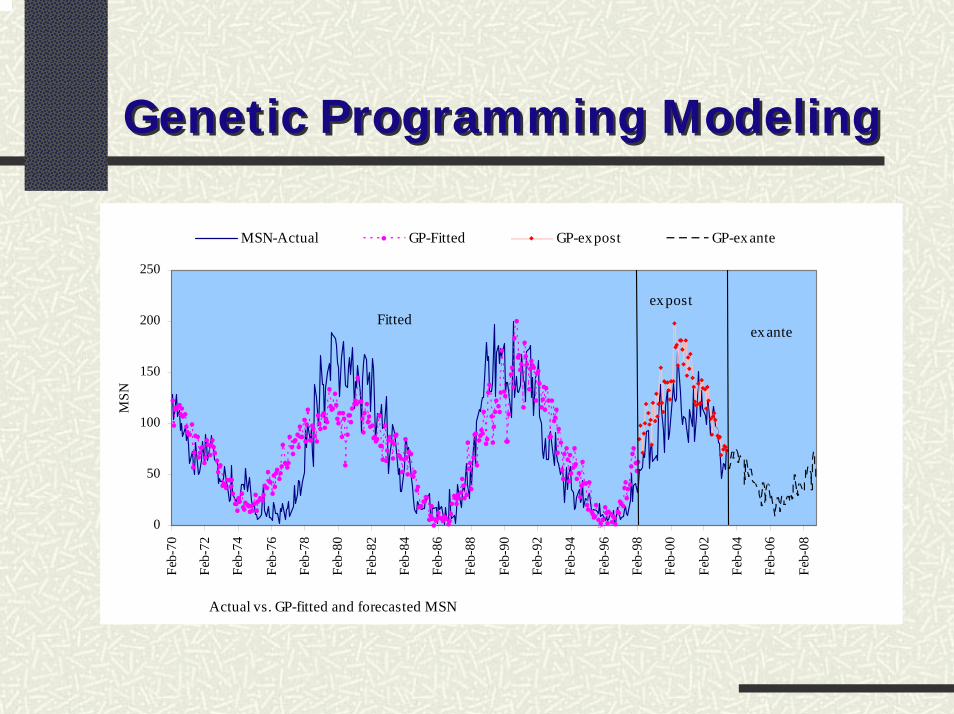
Genetic Programming ModelingGenetic Programming Modeling

Actual vs. GP-fitted and forecasted MSN

0

50

100

150

200

250

Feb-

70

Feb-

72

Feb-

74

Feb-

76

Feb-

78

Feb-

80

Feb-

82

Feb-

84

Feb-

86

Feb-

88

Feb-

90

Feb-

92

Feb-

94

Feb-

96

Feb-

98

Feb-

00

Feb-

02

Feb-

04

Feb-

06

Feb-

08

MSN

MSN-Actual GP-Fitted GP-ex post GP-ex ante

ex post

ex anteFitted

WaveletsThe DWT Haar Wavelet:

Consecutive pairs of observations are averaged (s1) and differenced (d1).The averaged (s1) resulting series is then averaged (s2) and differenced (d2).The process is repeated J times.

DWT is the Discrete Wavelet TransformIts inverse is the IDWT.

Daubechies Wavelets

The Haar Wavelet

• The Haar transform iteratively decomposes a sequence of observation into father and mother wavelets. The inverse transform restores the series to its original sequence.

• At each level of decomposition the two transforms are half the length they were in the prior one. In the Haar transform, a series Xt is first decomposed to obtain averages (denoted by a1) and differences (denoted by d1) of consecutive pairs of observations (as opposed to consecutive points) in that series. Averages preserve its main signal while differences capture the series’ fluctuations.

• If Xt contains T0 elements, there will be a1 and d1 of averages and differences of length T1 = T0/2. The input for the next level of decomposition is a1, where for this second iteration, T2 = T1/2. Recursive iterations continue until a single average and difference are calculated.

The Haar Wavelet (Cont’d)

The computations of aj,t and dj,t are as follows:

( ) 2aaa 1t21jt1jtj −−−+= ,,,

( ) 2aad 1t21jt1jtj −−−−= ,,,

The averages:

The differences:

where for each level of decomposition tj = 1, …, Tj-1/2, j = 1, …, J, and a0 = Xt.

The Haar Wavelet (Cont’d)

The inverse transforms are obtained by solving the previous equations for aj-1,t and aj-1,2t-1. Alternatively, these two equations

tjtj1t21j daa ,,, −=−−

tjtjt1j daa ,,, +=−

are computed until the original series is restored.

Haar in Excel

DWT of the Haar WaveletDWT of the Haar Wavelet

0 100 200 300 400 500

s4

d4

d3

d2

d1

idwt

Sunspot

data

Wavelets Transforms:Wavelets Transforms:

Haar transformations are obtained to use as input data to train using NN or fit using GP. To obtain those transformations, a level of scaling J must be selected first. J is selected such that there is a sufficiently large number of observations left at the Jth

level to use in model training or fitting. The sunspot numbers data set is sufficiently large. It was possible to use 512 observations to obtain the wavelet transformations. At J=4, the series used to model independently are d1, with T = 256; d2, with T = 128; d3, with T = 64; d4 and s4, with T = 32.

Obtaining the forecastsNN and/or GP are employed to obtain fits and forecasts of the five series (d1, d2, d3, d4, and s4).The inverse discrete wavelet transform (IDWT) is then used to compute the forecast of the observed series. IDWT must have identical number of observations in each of the five series. Values of the observations do not have to be identical to their originals. This makes it possible to replace historic with forecast values.

Example:s4 original training set observations 1 – 32

s4 fitted & forecasted set observations 9 – 40

Here values returned to complete the IDWT are the same number of observations but have different values.

1 32

9 40

Obtaining the forecasts (Cont’d)

d4 original training set d4 fitted & forecasted setHere values returned to complete the IDWT are

observations 9 to 40 instead of the original 1 to 32 values.

d3 original training set d3 fitted & forecasted setHere values returned to complete the IDWT are

observations 17 to 82 instead of the original 1 to 64 values.

And so on ….

1 32

9 40

1 64

17 82

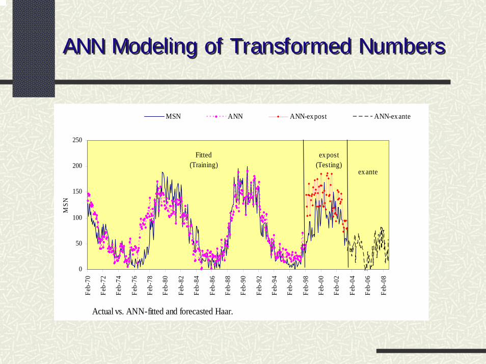
ANN Modeling of Transformed NumbersANN Modeling of Transformed Numbers

Actual vs. ANN-fitted and forecasted Haar.

0

50

100

150

200

250

Feb-

70

Feb-

72

Feb-

74

Feb-

76

Feb-

78

Feb-

80

Feb-

82

Feb-

84

Feb-

86

Feb-

88

Feb-

90

Feb-

92

Feb-

94

Feb-

96

Feb-

98

Feb-

00

Feb-

02

Feb-

04

Feb-

06

Feb-

08

MSN

MSN ANN ANN-ex post ANN-ex ante

ex post(Testing)

ex ante

Fitted (Training)

GP Modeling of Transformed NumbersGP Modeling of Transformed Numbers

Actual vs. GP-fitted and forecasted Haar.

0

50

100

150

200

250

Feb-

70

Feb-

72

Feb-

74

Feb-

76

Feb-

78

Feb-

80

Feb-

82

Feb-

84

Feb-

86

Feb-

88

Feb-

90

Feb-

92

Feb-

94

Feb-

96

Feb-

98

Feb-

00

Feb-

02

Feb-

04

Feb-

06

Feb-

08

MSN

MSN GP GP-ex post GP-ex ante

ex post

ex anteFitted

Application: Exchange Rate

0 50 100 150 200 250

s3

d3

d2

d1

idwt

DWT & IDWT of the exchange rate

Exchange Rates ForecastExchange Rates Forecast

Actual, f itted, & Haar forecasted Y/$ exchange rate

100

105

110

115

120

1 12 23 34 45 56 67 78 89 100 111 122 133 144 155 166 177 188 199 210 221Observat ions

Y/$Actual Predicted ex post ex ante

Actual, fitted, & GP forecasted Y/$ exchange rate

100

105

110

115

120

1 14 27 40 53 66 79 92 105 118 131 144 157 170 183 196 209 222Observations

Y/$ Actual Predicted ex post ex ante

Haar forecast of $/Yen exchange rate

MSE MAPE

Training 12/8/03 - 5/16/04 2.39 1.17

ex post 5/17/04 - 6/17/04 0.10 0.24

ex ante 6/18/04 - 7/19/04 17.66 3.41

Forecast Statistics

1.423.646/18/04 - 7/19/04ex ante

0.741.245/17/04 - 6/17/04ex post

1.282.9312/8/03 - 5/16/04Training

MAPEMSE

GP forecast of $/Yen exchange rate

Summary of ResultsSummary of Results

Wavelet conversions of series belonging to natural phenomena seems more promising than it is for financial time series, but more research is surely needed.Using long-lag structure works well with computational techniques and seems to have potential in providing reasonable long-into-the-future forecasts.GP & wavelet/GP forecasts seem more logical than ANN forecasts.