wavelet Transforms And Their Applications To...
64
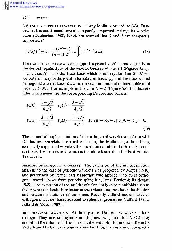
Annu. Rev. Fluid Mech. 1992.24 : 395-457 Copyright © 1992 by Annual ReviewsInc..~tll rights reserved WAVELET TRANSFORMS AND THEIR APPLICATIONS TO TURBULENCE Marie Farye LMD-CNRS Ecole Normale Sup6rieure, 24, rue Lhomond, 75231 Paris Cedex 5, France KEY WORDS: orthogonal bases, turbulence INTRODUCTION Wavelet transforms are recent mathematical techniques, based on group theory and square integrable representations, which allows one to unfold a signal, or a field, into both space and scale, and possibly directions. They use analyzing functions, called wavelets, which are localized in space. The scale decomposition is obtained by dilating or contracting the chosen analyzing wavelet before convolvingit with the signal. The limited spatial support of wavelets is important because then the behavior of the signal at infinity does not play any role. Therefore the wavelet analysis or syn- thesis can be performed locally on the signal, as opposed to the Fourier transform which is inherently nonlocal due to the space-filling nature of the trigonometric functions. Wavelet transforms have been applied mostly to signal processing, image coding, and numerical analysis, and they are still evolving. So far there are only two complete presentations of this topic, both written in French, one for engineers (Gasquet & Witomski 1990) and the other for mathematicians (Meyer 1990a), and two conference proceedings, the first in English (Combes et al 1989), the second in French (Lemari6 1990a). In preparation are a textbook (Holschneider 1991), a course (Dau- bechies 1991), three conference proceedings (Meyer & Paul 1991, Beylkin et al 1991b, Farge et al 1991), and a special issue of IEEETransactions 395 0066-4189/92/0115-0395502.00 www.annualreviews.org/aronline Annual Reviews
Transcript of wavelet Transforms And Their Applications To...
Annu. Rev. Fluid Mech. 1992.24 : 395-457Copyright © 1992 by Annual Reviews Inc..~tll rights reserved
WAVELET TRANSFORMS ANDTHEIR APPLICATIONS TOTURBULENCE
Marie Farye
LMD-CNRS Ecole Normale Sup6rieure, 24, rue Lhomond,75231 Paris Cedex 5, France
KEY WORDS: orthogonal bases, turbulence
INTRODUCTION
Wavelet transforms are recent mathematical techniques, based on grouptheory and square integrable representations, which allows one to unfolda signal, or a field, into both space and scale, and possibly directions. Theyuse analyzing functions, called wavelets, which are localized in space. Thescale decomposition is obtained by dilating or contracting the chosenanalyzing wavelet before convolving it with the signal. The limited spatialsupport of wavelets is important because then the behavior of the signalat infinity does not play any role. Therefore the wavelet analysis or syn-thesis can be performed locally on the signal, as opposed to the Fouriertransform which is inherently nonlocal due to the space-filling nature ofthe trigonometric functions. Wavelet transforms have been applied mostlyto signal processing, image coding, and numerical analysis, and they arestill evolving.
So far there are only two complete presentations of this topic, bothwritten in French, one for engineers (Gasquet & Witomski 1990) and theother for mathematicians (Meyer 1990a), and two conference proceedings,the first in English (Combes et al 1989), the second in French (Lemari61990a). In preparation are a textbook (Holschneider 1991), a course (Dau-bechies 1991), three conference proceedings (Meyer & Paul 1991, Beylkinet al 1991b, Farge et al 1991), and a special issue of IEEE Transactions
3950066-4189/92/0115-0395502.00
www.annualreviews.org/aronlineAnnual Reviews

396 FARGE
on Information Theory (Daubechies et al 1991), which are all written English.
Therefore, I assume that the reader is not yet familiar with this topicand give a general presentation of both the continuous wavelet transformand the discrete wavelet transform, in a manner as complete and detailedas possible, to provide the reader with the basic information with whichto start using these transforms. In this spirit I will discuss the choice of thewavelet, which varies according to its application, and point out pitfallsto be avoided in the interpretation of wavelet transform results.
Since most of the existing work has so far been of an exploratorycharacter and thus cannot be held as representative of the possible impactof wavelets on fluid mechanics, only brief reference will be made to papersdealing with applications. I shall also present several new diagnostics, allbased on wavelet coefficients, which may be useful to analyze, model, orcompute turbulent flows.
1. THE NEED FOR A SPACE-SCALE
DECOMPOSITION OF TURBULENT FLOWS
In the field of turbulence, one may feel uneasy about the fact that we havetwo different pictures of turbulence, depending on the side of the Fouriertransform from which we perceive it. On the one hand, if we look at theFourier spectral space, we have a theory that assumes the existence of anenergy cascade between the different excited wavenumbers of the flow. Itpredicts the universality of the Fourier energy spectrum in the inertialrange, namely for wavenumbers larger than those corresponding to theintegral scales at which the flow is excited and smaller than those cor-responding to the dissipative scales where all instabilities are damped. Inthis Fourier space approach the direct numerical simulation of a turbulentflow requires a number of resolved Fourier wavenumbers which scales asRe for two-dimensional flows and as Re9/4 for three-dimensional flows (Rebeing the Reynolds number characteristic of the flow turbulence). On theother hand, if we look at the physical space, we must admit a lack ofgeneral theory. Still, we have a large amount of evidence, both experi-mental (Townsend 1956, Kline et al 1967, Laufer 1975) and numerical(Basdevant et al 1981, McWilliams 1984, Kim et al 1987), for the presenceof coherent structures in turbulent flows. They correspond to the con-densation of the vorticity ficld into organized patterns, which contain mostof the energy--or enstrophy in dimension two--of the flow and wherenonlinearity is reduced, or even cancelled when the coherent structures areaxisymmetric. These coherent structures seem to play an important, butnot yet well understood, dynamical role. We can ask the following ques-
www.annualreviews.org/aronlineAnnual Reviews

WAVELET TRANSFORMS 397
tions. Are there some elementary coherent structures? Do their mutualinteractions have a universal character? Is it possible to compute the flowevolution with a reduced number of degrees of freedom relative to the verylarge number of Fourier components otherwise necessary? This reductioncould correspond to a projection of Navier-Stokes equations on thosecoherent structures or on some related functional bases well localized inphysical space.
Being very uncomfortable with these two separate descriptions of tur-bulence, I was immediately enthusiastic when, in 1984, A. Grossmann toldme about the wavelet transform theory he was developing from Morlet’soriginal ideas. His theory had the promise of a unified approach whichcould reconcile these two descriptions and allow us to analyze a turbulentflow in terms of both space and scale at once, up to the limits of theuncertainty principle. Another reason, rather naive, for the immediateappeal of wavelets was the fact that the Morlet wavelet evoked to me theshape of Tennekes and Lumley’s eddy (Tennekes & Lumley 1972) pro-posed to model turbulence, and of some coherent structures whose exis-tence had been conjectured by Ruelle (D. Ruelle, personal communication,1983) and then observed by Basdevant in his numerical simulations oftwo-dimensional flows (Basdevant & Couder 1986). Indeed, it seems muchbetter to decompose a turbulent field into such localized oscillations offinite energy as wavelets, rather than into space-filling trigonometric func-tions which do not belong to the L2(IIn) functional space and therefore arenot of finite energy.
In the context of turbulence, the wavelet transform may yield someelegant decompositions of turbulent flows (Section 5.1). The continuouswavelet transform offers a continuous and redundant unfolding in termsof both space and scale, which may enable us to track the dynamics ofcoherent structures and measure their contributions to the energy spectrum(Section 5.2). The discrete wavelet transform allows an orthonormal pro-jection on a minimal number of independent modes which might be usedto compute or model the turbulent flow dynamics in a better way thanwith Fourier modes (Section 5.3).
2. WAVELET TRANSFORM PRINCIPLES
2.1 History
The wavelet transform originated in 1980 with Morlet, a French researchscientist working on seismic data analysis (Morlet 1981, 1983; Goupillaudet al 1984), who then collaborated with Grossmann, a theoretical physicistfrom the CNRS in Marseille-Luminy. They developed the geometricalformalism of the continuous wavelet transform (Grossmann et al 1985,
www.annualreviews.org/aronlineAnnual Reviews

398 FARGE
1986, 1987, 1989; Grossmann 1988; Grossmann & Morlet 1984, 1985;Grossmann & Paul 1984; Grossmann &Kronland-Martinet 1988) basedon invariance under the affine group namely translation and dilation--which allows the decomposition of a signal into contributions of both spaceand scale (Section 3.1). In particular the continuous wavelet transform well suited for analyzing the local differentiability of a function, and fordetecting and characterizing its possible singularities (Holschneider 1988b;Jaffard 1989a; Arn6odo et al 1988; Holschneider & Tchamitchian 1989;Mallat & Hwang 1990; Jaffard 1991a,b). It is also useful for signal process-ing, in particular with the "skeleton" technique (Escudi6 & Torr6sani 1989,Tchamitchian & Torrbsani 1991, Delprat et al 1991) which allows theextraction of the modulation law of a complex signal, assuming somestationary phase hypothesis. The continuous wavelet transform has beenextended to n dimensions by Meyer (1985) and then by Murenzi usingrotation, in addition to dilation and translation (Murenzi 1989, 1990;Antoine et al 1990, 1991). Murenzi is presently extending it to n dimensionsplus time (Duval-Destin & Murenzi 1991). The wavelet transform thenworks as a "microscope," discriminating different scales in an n-dimen-sional field, and as a "polarizer," separating the different angular con-tributions of the signal.
When, in 1985, Meyer read Morlet and Grossmann’s work, he recog-nized Calderon’s identity (Calderon 1964) behind the admissibility con-dition and the reconstruction formula of the continuous wavelet theory(Section 3.1). He then collaborated with Grossmann and Daubechies(Daubechies et al 1986) to select a discrete subset of the continuous waveletspace, chosen in such a way that it constitutes a quasi-orthogonal completeset of Lz(Rn), called a wavelet frame (Section 4.1). Complementary to this,Morlet and Grossmann had previously defined an interpolation formula--based on the reproducing kernel property Of the continuous wavelet trans-form (Section 3.2)--which recovers the whole space of continuous waveletcoefficients from the coefficients of a discrete subset, such as a waveletframe (Grossman & Morlet 1985). Meyer then tried to prove that, evenif wavelet decomposition behaves in some sense as an orthogonal basis ofL2(R"), there could not be any true orthogonal basis constructed withregular wavelets. The Haar orthogonal basis (Haar 1909) was well-known,but the lack of regularity of the functions it uses creates problems fordecomposing smooth functions, whose Haar coefficients would only decayvery slowly at infinity. Meyer was therefore surprised to discover anorthogonal basis (Section 4.2) built from a regular wavelet (Meyer 1986,1987if, b, 1988). He later extended it to the n-dimensional case in col-laboration with his student Lemari+ (Lemari6 & Meyer 1986). In 1987,Meyer (1988, 1989a,b,c, 1990a,b,c) and Mallat (1988) introduced the
www.annualreviews.org/aronlineAnnual Reviews

WAVELET TRANSFORMS 399
cept of multiresolution analysis, which is very similar to the Quadratic MirrorFilters technique (Esteban & Galand 1977) defined in digital processingand computer vision. This approach gives a general method for buildingorthogonal wavelet bases and leads to the implementation of fast waveletalgorithms (Mallat 1989a,b). Since then many other orthogonal waveletbases have been found, among them: the Battle-Lemari6 wavelet (Battle1987, 1988; Lemari6 1988), which uses exponentially decreasing splinefunctions, the discrete orthogonal bases of Rioul (1987, 1991), and thecompactly supported and regular wavelets of Daubechies (1988, 1989),built by iterating some discrete filters.
From today’s point of view we can recognize, a posteriori, that severalaspects of wavelet theory were already present, more or less explicitly, inmany fields, such as image processing (Granlund 1978), because this kindof decomposition is indeed very natural. This is particularly clear for theStr6mberg orthogonal basis (Str6mberg 1981) used in functional analysisand for the hierarchical basis of Zimin proposed to model turbulence(Zimin 1981). Today wavelet theory is a new and rapidly evolving math-ematical technique, which has established similarities between variousmethods that were independently developed in different fields, from func-tional analysis to signal proccssing, and gives them a common theoreticalframework.
2.2 Definition
What are the necessary ingredients of the wavelet transform?
ADMISSIBILITY TO be called a "wavelet," the analyzing function shouldbe admissible (Section 3.1), which, for an integrable function, means thatits average should be zero. This requirement excludes, for instance, func-tions used in Karhunen-Lo6ve--also called Proper OrthonormalDecompositions (Lumley 1981, Aubry et al 1988)--which are not of zeromean value.
SIMILARITY The scale decomposition should be obtained by the trans-lation and dilation of only one "mother" function. All analyzing waveletsshould therefore be mutually similar, namely scale covariant with oneanother, in particular they should have a constant number of oscillations(Section 3.1). Thus this dilation procedure allows an optimal compromisein view of the uncertainty principle: The wavelet transform gives very goodspatial resolution in the small scales and very good scale resolution in thelarge scales (Figure 1). This similarity condition excludes the windowedFourier transform of Gabor (1946), whose scale decomposition, is basedon a family of trigonometric functions exhibiting increasingly many oscil-
www.annualreviews.org/aronlineAnnual Reviews

400 FARGE
iI
Figure 1 Phase space associated with different transforms. The uncertainty principleimposes phase-space "atoms" such that Ax" Ak > 2n. 1. Analyzing function in physicalspace, 2. analyzing function in Fourier space, and 3. information cell Ax--Ak in phase space.(a) Shannon sampling, (b) Fourier transform, (c) Gabor transform, (d) Wavelet transform.
lations in a window of constant size. In this case the spatial resolution inthe small scales and the range in the large scales are limited by the size ofthe window (Figure 1).
TNVER3rmTLT3:’¢ There should be at least one reconstruction formula forrecovering the signal exactly from its wavelet coefficients and for allowingthe computation of energy or other invariants directly from them (Sections3.1 and 4.2). This precludes passband filtering techniques, renamed today
www.annualreviews.org/aronlineAnnual Reviews

WAVELET TRANSFORMS 401
"Fourierlets," which do not give an exact reconstruction formula forsynthesizing the signal from its spectral coefficients.
REGULARITY In practice the wavelet should also be well localized on bothsides of the Fourier transform, namely it should be concentrated on somefinite spatial domain and be sufficiently regular. Indeed, there also existregular wavelets that vanish outside a domain of compact support (Section4.2). This additional regularity requirement excludes all discontinuousfunctions such as those used in the Haar orthogonal decomposition (Haar 1909).
CANCELLATIONS For some applications, in particular turbulent signalanalysis, the wavelet should not only be of zero mean value (admissibilitycondition), but should also have some vanishing high-order moments(Section 3.1). This requirement, which eliminates the most regular (poly-nomial) part of the signal, allows the study of its high-order fluctuationsand possible singularities in some high-order derivatives. In this case, thewavelet coefficients will be very small in the regions where the function isas smooth as the order of cancellation and the wavelet transform will onlyreact to the higher order variations of the function.
2.3 Compar&on with the Fourier Transform
Since Fourier’s work on heat theory, the most commonly used basisfunctions in physics have been the trigonometric functions, because theyconstitute an orthogonal basis of L2(0, 2~), the functional space of squareintegrable functions. Thus they allow the decomposition of any functionf(x) c L2(O, 2r0 into a linear combination of Fourier vectors, defined bytheir Fourier coefficients f(k) = (eik~lf(x)). Unfortunately the trigono-metric functions oscillate forever and therefore the information contentoff(x) is completely delocalized among all the spectral coefficients f(k).Indeed the Fourier transform does not lose information about f(x), butinstead "spreads" it away; it is then very difficult, or even impossible, assoon as there is some computational noise, to study the properties off(x)from those off(k). Let us for instance take the case of a function that smooth everywhere except at a few singular points. The positions of thesingularities are related to the phase of all the Fourier coefficients. There-fore there is no way to localize the singularities in Fourier space and theonly solution will be to reconstructf(x) fromf(k). Similarly, this functionf(x) will have a power-law spectrum so that the modulus of the Fouriercoefficients will scale as k ~. This indicates thatf(x) is globally nonregularwith singularities of at most exponent e. Unfortunately, we have then lostthe essential information, namely the fact thatf(x) is regular everywhereexcept at a few singular points. If, for instance, these singular points are
www.annualreviews.org/aronlineAnnual Reviews
402 FARGE
due to experimental errors, we will not be able to filter them out becausethey have affected all the Fourier coefficients.
In contrast to the Fourier transform, the wavelet transform keeps thelocality present in the signal and allows the local reconstruction of a signal.It is then possible to reconstruct only a portion of it or only its localcontributions to a given range of scales. In fact, there is a relationshipbetween the local behavior of a signal and the local behavior of its waveletcoefficients. For instance, if a function f(x) is locally smooth, the cor-responding wavelet coefficients will remain small, and iff(x) contains singularity, then in its vicinity the wavelet coefficients’ amplitude willincrease drastically (Section 3.2). Likewise the wavelet series off(x) verges locally to f(x), even if f (x) is a distribution (in this case the orderof the distribution should not exceed the regularity of the analyzing wave-let). By "locally" we mean that, for reconstructing a portion of a signal,it is only necessary to consider the wavelet coefficients belonging to thecorresponding subdomain of the wavelet space, the so-called influencecone (Section 3.2). Consequently, the wavelet transform is very robust forreconstruction. Indeed, if the wavelet coefficients are occasionally subjectto errors, this will only affect the reconstructed signal locally near theperturbed positions, while the Fourier transform would spread out theerrors everywhere in the reconstructed signal. The Fourier transform isalso particularly sensitive to phase errors, due to the alternating characterof the trigonometric series. This is not the case for wavelet transforms. Itis even possible to correct the errors present in the continuous waveletcoefficients, thanks to the built-in redundancy of the continuous wavelettransform duc to its reproducing kernel property (Section 3.1).
In fact the wavelet transform is not intended to replace the Fouriertransform, which remains very appropriate, for instance, in the study ofharmonic signals or when there is no need for local information. Let usalso mention that the Fourier transform plays a role in the admissibilitycondition defining wavelets (Section 3.1) and in the construction of discretefilters used in multiresolution analysis (Section 4.2). In practice the Fouriertransform may be thought of as imbedded into the wavelet transform,because it is, to first approximation, possible to compute the Fourierspectrum of a signal by summing its wavelet coefficients over all positionsscale by scale (Section 5.2).
3. THE CONTINUOUS WAVELET TRANSFORM
3.1 Analysis and Synthesis
WAVELET DEFINITION The only constraint imposed on a function ~b(x),real or complex valued, in order to be a wavelet is the admissibilitycondition which requires:
www.annualreviews.org/aronlineAnnual Reviews
k 2dnk
with
~(k) = (2~)-" ~R" ~b(X) e-v/Z~k’x
WAVELET TRANSFORMS 403
(1)
n being the number of spatial dimensions. If ~b(x) is integrable this actuallyimplies that it has zero mean:
fa~(x)d"x = 0 or ~(Ikl = 0) (2)
In practice the wavelet should also be well-localized in both physical andFourier spaces. If one wants to study the behavior of the Mth derivativeoff(x), the wavelet should have cancellations up to order M, in order thatit does not react to the lower-order variations off(x), namely we shouldhave:
fR"~O(x)xm d"x = (3)
for all m _< M.
WAVELET ANALYSIS From this function ~, the so-called mother wavelet,we generate the family of continuously translated, dilated, and rotatedwavelets:
./2¢[-a-, x- x’-I= l- [_ (0) ~J, (4)
with lc R+ as the scale dilation parameter corresponding to the width ofthe wavelet and x’ e R" as the translation parameter corresponding tothe position of the wavelet; l and x’ are dimensionless variables. In thecontinuous wavelet literature the scale is denoted by a and the position byb to recall that this transform is based on the affine group ax÷b. Weprefer here to denote the scale l, because it corresponds to the length scaleat which we analyze f(x), and the position of the analyzing wavelet x’,because it indeed corresponds to the actual position in physical space; wemust distinguish x’ and x, which will be used as an integration variable in(6). The rotation matrix ~ belongs to the group SO(n) of rotations R", and depends on the n(n-1)/2 Euler angles 0. The factor l -"/z is anormalization which causes all the wavelets to have the same L2 norm;
www.annualreviews.org/aronlineAnnual Reviews

404 FARGE
therefore all wavelets will have the same energy and the wavelet coefficientswill correspond to energy densities.
The admissibility condition (I) implies that the Fourier transform of is rapidly decreasing near k = 0. Therefore the Fourier transform of thefamily ~tx.0 constitutes a bank of passband filters with constant ratio ofwidth to center frequency:
q~tx,00’) = Z"/2~[t f~- ’(0)k] e-,/:~k’,’. (~)
To summarize, the family of analyzing wavelets ~;~,0 may be compared toa mathematical microscope and polarizer, for which ~ characterizes theoptics, l- ~ is the resolution, x’ the position, and 0 the polarization angle.
The continuous wavelet transform of a function or a distribution f(x)is the LZ-inner product betweenfand the wavelet family ~;~,0, which givesthe wavelet coefficients:
f(l, x’, O) = ($,~.olf) = ~ f(x)$~.0(x) (6)n
where $* is the complex conjugate of $, or likewise the inner productbetween~and the filter bank @~’0, which gives:
f(l, x’, 0) = f f(k)ff~.0(k) (7)n
Figure 2 shows the continuous wavelet transform of some "academic"signals chosen as limiting cases of a hypothetical turbulent signal: a deltafunction, a period-doubling signal, and a Gaussian white noise signal.
WAVELET SVNX~S~S The admissibility condition (1) implies the existenceof a reproducing kernel (which will be defined in Section 3.2). We cantherefore recover the signalf(x) from its wavelet coefficients:
f(x) = c~’ +. .~(~,x’,0)~..0(x) i.+, (8)
If @ is complex-valued andfreal-valued we should only take the real parto~(8).
For one-dimensional or for isotropic wavelets we need not integrateover angles. Otherwise we would have to carry out the following procedure.In order to integrate over the n(n-I)/2 Euler angles 0, we define theintegral:
o) .... (~ ,~ ...... (,~... ~(o). (9)0
www.annualreviews.org/aronlineAnnual Reviews

406 FARGE
In this integral we use the invariant measure d#(O) of the rotation groupSO(n) defined as:
n--1 k
= ’~dO~. (10)did(O) A. I-[ YI sin J- Ojk--lj--I
with
k= ! 27~k/2
and the Euler angles
50_<0~<2~z for k~[1,n-1],
_<0~<~ for j#landk~[1,n-1].
By analogy with Fourier space, we shall call "wavelet space" the set offunctionsfthat are wavelet transforms of f for a given wavelet
The continuous wavelet transform isometrically transforms a functionof n variables into, either an (n+ 1)-dimensional wavelet space if we usean isotropic wavelet, or an {n[(n + 1)/2] + 1 }-dimensional wavelet space we consider a directional wavelet. Therefore the information contained inthe wavelet coefficients is redundant, which is expressed by the reproducingkernel property of the continuous wavelet transform (Section 3.2); conse-quently there exist many different reconstruction formulas. For instance,it is possible to reconstructf(x) from its wavelet coefficients using anotherfunction, the synthesizing wavelet, different from the analyzing wavelet,which then must verify a modified admissibility condition (Holschneider1988a, Holschneider & Tchamitchian 1989). We can even choose a dis-tribution such as the delta function (b) to reconstruct the signal. In thiscase we get the simple reconstruction formula, found empirically by J.Morlet:
f(x) = 1 ÷f( l,x,O)~d#(O) (11)
with
c~ ; (2~)~j2
We mention incidentally that we can use a wavelet to synthesize a signalfrom what are called its Radon transform coefficients, which may beinteresting for tomographic applications (Holschneider 1990).
www.annualreviews.org/aronlineAnnual Reviews
WAVELET TRANSFORMS 407
3.2 Elementary Properties
We will now list some of the main properties of the continuous wavelettransform. For the sake of simplicity, from here on we will consider theone-dimensional wavelet transform, the generalization to n dimensionsbeing straightforward, and discard the prime in x’. We will denote thecontinuous wavelet transform of a functionf(x) by the operator notationW[f](x), and the resulting wavelet coefficients by f(l, x).
LINEARITY The wavelet transform is linear because it is an inner productbetween the signal f and the wavelet ~O. Likewise, the continuous wavelettransform of a vector function is a vector whose components are thecontinuous wavelet transform of the different components.
COVARIANCE BY TRANSLATION AND DILATION The continuous wavelettransform is covariant under any translation x0:
W[f] (x-- Xo) = f(1, x-- Xo), (12)
which in particular implies that differentiation commutes with continuouswavelet transform; namely we have
c?~ W ( f ) = W ~x
V[W(f)] = W(Vf),
V.[W(f)] = W(V.f). (13)
A consequence of the translation covariance is the fact that the frequencyof a monochromatic signal can be read off from the phase of the waveletcoefficients (Escudi6 & Torrtsani 1989, Guillemain 1991, Tchamitchian Torrtsani 1991, Delprat et al 1991). The number of zeros of the phase onlines with l = constant gives the frequency of the signal (Figure 2b). Thisproperty is independent of the wavelet chosen.
The continuous wavelet transform is also covariant under any dilationby/0:
IV[f] (lox) = IF 1.y(/0/, lox). (14)
A consequence of the dilation covariance is the fact that the wavelettransform of a power-law function is fully determined by its restriction toany line l = constant. The lines of constant phase point out the possiblesingularities of the function (Figure 2a). This property is also independentof the wavelet choice.
www.annualreviews.org/aronlineAnnual Reviews

408 FARGE
DIFFERENTIATION
IOmf l~+ oo am
W ~m = (- 1)"~ f(x)~[~.*~t(x)] (15)
ENERGY CONSERVATION
lf(x)lZdx = l If(l,x)l’lf (/,x)l ~ (16)
The wavelet transform conserves energy not only globally but also locallyif one considers all coefficients inside the "influence cone" which consistsof the spatial support of all dilated wavelets. The above relation cor-responds to energy conservation, which is a generalization of the Plan-cherel identity to the continuous wavelet transfo~. It implies that thereis no loss of information in transforming the signal into its waveletcoefficients.
The total energy can also be split among the different scales l:
f_~ ~2dx
~(~) = C&’ ~ lf(i,x)l
spac~-scaL~ ~oc~Tv The space-scale locality of the analyzing wavelet~ leads to the conservation of locality in the wavelet coefficient space, incontrast to the Fourier transfo~ which loses the locality present in thesignal. For instance, if @ is well-localized in the space interval a~ for l = 1,then the wavelet coefficients corresponding to the position x0 will all becontained in the influence cone defined by x ~ [x0-(l" a~)/2, x0 + (l" a~)/2].This cone corresponds to the spatial support of all dilated wavelets at thepoint x0. Likewise, if ~ is well-localized in the Fourier interval Ak around
k~ for l = 1, then the ~avelet coefficients corresponding to the Fourierfrequency k0 in the signal will only be contained in the subband definedby ~ [kAk0+(ak/20) ’, ~(~0-(ak/~t))-’].
LOCAL REGULARITY ANALYSIS One of the most interesting properties ofthe continuous wavelet transfo~, implied by its dilation covariance, isthe possibility it offers to measure the local regularity of a function andtherefore to characterize the functional space to which it belongs (Hol-schneider 1988a,b; Jaffard 1989a,b, 1991c; Holschneider & Tchamitchian1989, 1990; Tchamitchian 1989c). For instance iff~Cm(xo), i.e. iff iscontinuously differentiable in x0 up to order m, then
~(l, xo) ~ lm+~P/2 for l~0. (18)
The factor l ~/~ comes from the fact that, due to the scale invariance (14),
www.annualreviews.org/aronlineAnnual Reviews
WAVELET TRANSFORMS 409
if we want to study the scaling of a function we must take the waveletcoefficients in the L~ norm, instead of L2. The wavelet coefficients writtenin the Lt norm are related to the wavelet coeff~cients written in the L2
norm by the simple expression:
fL’ = l-1/2yL2. (19)
Iffbelongs to A~(x0), the H61der space of functions of exponent ~, i.e. f is continuous, not necessarily differentiable in x0 but such that
If(x+xo)-f(x)[ = Clxol ~ with g < 1 and constant C > 0, (20a)
then
3~(/, x0) Ce’f~*l~l 1/~ for l ~ 0, (20b)
where @ is the phase of the wavelet coefficients.The transformed function f is regular even iff is not. The information
about any possible singularities present in the signal, their position x0,their strength C, and their scaling exponent ~, is given by the asymptoticbehavior off(l, xo), written in norm L~ (19), for l tending to zero. If theL~-norm wavelet coefficients diverge in the small scales at the point Xo,then f is singular at x0 and the slope of log If(l, x0) l versus log l will givethe exponent of the singularity (20). It is also very easy to localize thepossible singularities off by looking at the phase of its wavelet coefficients:The lines of constant phase converge on the singularities (Figure 2a). If,on the contrary, the modulus of the wavelet coefficient becomes zero inthe very small scales around xo, then the functionf is regular at x0. Thisresult is in fact the converse of (18), but its mathematical justificationrequires more global assumptions on the analyzed function, namely somedecay of its wavelet coefficients in the vicinity of x0 (Jaffard 1989a). There-fore, in practice, to locally analyze a singularity at x0 we should first verifythat at small scales the wavelet coefficients around x0 are not larger thanthose at x0. Then we should consider not only the coefficientsf(l, x0), butat least all coefficients belonging to the influence cone pointing towardsx0. Those properties are independent of the choice of the wavelet andthey are particularly useful for characterizing fractals and multifractals(Holschneider 1988b; Arn+odo et al 1989; Ghez & Vaienti 1989; Argoulet al 1988, 1990; Falconer 1991; Freysz et al 1990).
REPRODUCING KERNEL Using the wavelet ~k, we can decompose any func-tion or distribution f into its wavelet coefficients. In the case of thecontinuous wavelet transform these coefficients form an over-completebasis. This implies a correlation between the wavelet coefficients which, inturn, corresponds to the existence of a reproducing kernel K6 associatedto the wavelet ~ defined by
www.annualreviews.org/aronlineAnnual Reviews
410 FARGE
K~(l,, 12, x’~, x’~) = ~ O,,x;O~x’~ dx. (21)
K~ characterizes the correlation of the continuous wavelet transformbetween two different points of the continuous half-plane (l, x). Its struc-ture depends on the choice of the wavelet; indeed the reproducing kernelmeasures the space and scale selectivity of each wavelet ~,~ and will there-fore be very useful in helping to choose the wavelet most appropriate to agiven problem.
Reciprocally, an arbitrary function]’of the half-plane (/, x)¯ + x R)isnot in general the wavelet transform of some function of R with respectto a given wavelet ~. This will hold only if]’is square integrable and satisfiesthe reproducing kernel equation (Grossmann et al 1989, Grossmann Kronland-Martinet 1988):
]’(l~x’) = .~o+ j- ~ g~,(l~, 12, x’~, xl) f(12, xl) dl2l ~dx’~
This condition should be checked if we want to partially resynthesize asignal from a filtered subset of its wavelet space. An important consequenceof the reproducing kernel property (22) is the fact that the continuouswavelet transform of a random signal (Figure 2c) shows some correlationsthat are obviously not in the signal, but in the wavelet transform itself.The size of the correlated regions is given by the reproducing kernel anddecreases with the scale. This is one of the most common pitfalls of thecontinuous wavelet transform and one should be particularly aware of itwhen studying turbulent signals. In the case of discrete orthogonal wavelettransform (Section 4.2) this problem no longer exists, since by definitionof orthogonality all wavelet coefficients are uncorrelated.
3.3 Implementation
WAVELET CHOICE AS we have seen, the wavelet transform is an innerproduct between an analyzing wavelet at a given scale 1 and the signal tobe analyzed; therefore the wavelet coefficients combine information aboutboth the signal and the wavelet. The choice of the transform, orthogonalor not, and of the appropriate wavelet is thus an important issue whichdepends on the kind of information we want to extract from the signal.For analyzing purposes the continuous wavelet transform is better suitedbecause its redundancy allows good legibility of the signal’s informationcontent. For compression or modeling purposes, the orthogonal wavelettransform (Section 4.2) or the newly developed wavelet packet technique(Section 4.3) are preferable because they decompose the signal into
www.annualreviews.org/aronlineAnnual Reviews

WAVELET TRANSFORMS 411
minimal number of independent coefficients. Then for choosing the appro-priate wavelet, we must look at its reproducing kernel (21), which charac-terizes its space, scale, and angular selectivity.
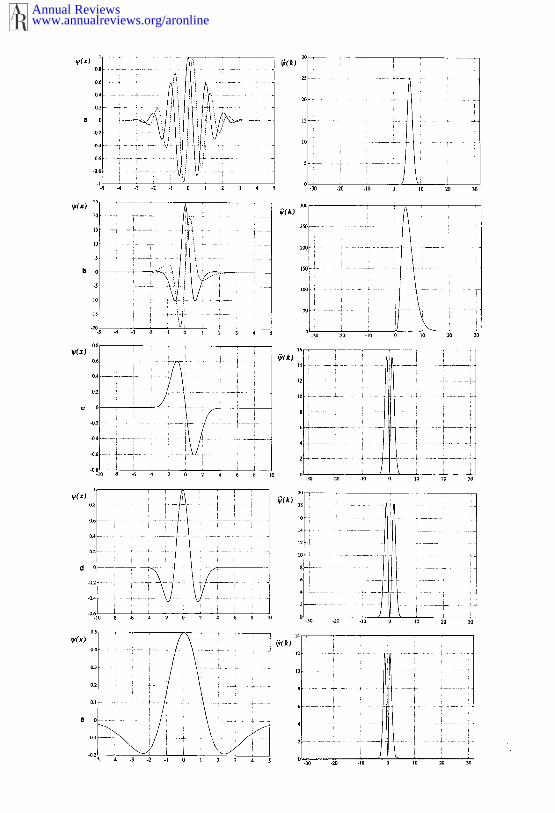
EXAMPLES OF COMPLEX-VALUED WAVELETS Let us consider the analysis ofa real-valued signal such as those encountered in fluid mechanics. In thiscase, we usually choose a continuous wavelet transform with a progressivecomplex-valued wavelet, because the quadrature n/2 phase shift between itsreal and its imaginary parts allows us to eliminate the wavelet’s oscillationswhen visualizing the wavelet coefficient modulus (Figure 2). From theresulting complex-valued wavelet coefficients we can thus separate the L2-
modulus, which gives the energy density, and the phase, which detectssingularities and measures instantaneous frequencies (Escudi6 & Torr6sani1989, Tchamitchian & Torr6sani 1991, Guillemain 1991, Delprat et al1991). As already stated, the lines of constant phase converge on singu-larities and the number of zero-crossings on lines l = constant, if the latterare parallel, is related to the signal frequency. The phase behavior isindependent of the choice of wavelet.
The most commonly used complex-valued wavelet is the Morlet wavelet(Figure 3a).
O(x) = e’J-2S~o "~ e-(Ixl:/2), (23)
which is a plane wave of wavevector k6, modulated by a Gaussian envelopeof unit width. Incidentally, the Morlet wavelet is only marginally admis-sible, because it is of zero average only if some very small correction termsare added. In practice, if we take [kol = 6, the correction terms becomeunnecessary because they are of the same order as typical computer round-off errors. Another way to ensure admissibility is to impose ~7(0) = 0. Fourier space, the Morlet wavelet is given by:
{~(k) = (2z)- ,/2 e-(k-t:¢,)2/2 for k > O,
~ (k) for k G O.(24)
A very interesting property of the Morlet wavelet in its generalization ton dimensions is its angular selectivity, which gets better and better as I k, Iincreases, but with a concomitant reduction in its spatial selectivity. Inorder to have both, angular and spatial selectivity Antoine and coworkershave proposed to elongate the Morlet wavelet, while keeping I kol smallenough to ensure a good space localization (Antoine et al 1990, Antoineet al 1991).
Another complex-valued wavelet, mostly used in quantum mechanics
www.annualreviews.org/aronlineAnnual Reviews
w(x)
w(x)
-30 -20 -10 0 10 2O 30
www.annualreviews.org/aronlineAnnual Reviews
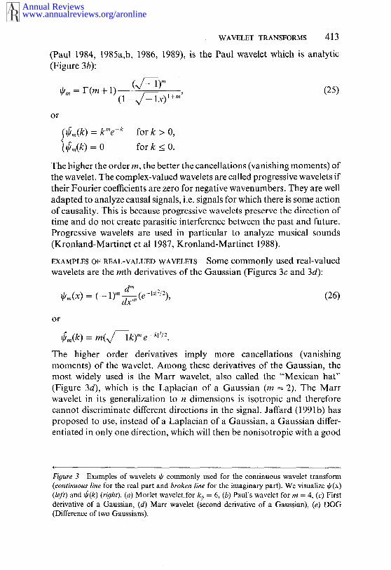
(Paul 1984, 1985a,b, 1986,(Figure 3b):
~/m = F(m+l) (%~l)m(1 -,fS x)’+m’
or
WAVELET TRANSFORMS 413
1989), is the Paul wavelet which is analytic
(25)
{~m(k) kme k fork > 0,
~,,,(k) = for k _< 0.
The higher the order rn, the better the cancellations (vanishing moments) the wavelet. The complex-valued wavelets are called progressive wavelets iftheir Fourier coefficients are zero for negative wavenumbers. They are welladapted to analyze causal signals, i.e. signals for which there is some actionof causality. This is because progressive wavelets preserve the direction oftime and do not create parasitic interference between the past and future.Progressive wavelets are used in particular to analyze musical sounds(Kronland-Martinet ct al 1987, Kronland-Martinct 1988).
EXAMPLES OF REAL-VALUED WAVELETS Some commonly used real-valuedwavelets are the ruth derivatives of the Gaussian (Figures 3c and 3d):
I[Im(X ) = (-- 1) m ~(d--lx12/2), (26)ax
or
~ffm(k) m(~-- lk)m e-Ikl2/2.
The higher order derivatives imply more cancellations (vanishingmoments) of the wavelet. Among these derivatives of the Gaussian, themost widely used is the Marr wavelet, also called the "Mexican hat"(Figure 3d), which is the Laplacian of a Gaussian (m ~ 2). The wavelet in its generalization to n dimensions is isotropic and thereforecannot discriminate different directions in the signal. Jaffard (1991 b) hasproposed to use, instead of a Laplacian of a Gaussian, a Gaussian differ-entiated in only one direction, which will then be nonisotropie with a good
Figure 3 Examples of wavelets ~b commonly used for the continuous wavelet transform(continuous line for the real part and broken line for the imaginary part). We visualize ~b(x)
(left) and ~(k) (right). (a) Morlet wavelet, for k~ = 6, (b) Paul’s wavelet for m = 4, (c) Firstderivative of a Gaussian, (d) Marr wavelet (second derivative of a Gaussian), (e) (Difference of two Gaussians).
www.annualreviews.org/aronlineAnnual Reviews
414 FARGE
angular selectivity. Antoine and co-workers have proposed to elongate itto recover some angular selectivity (Antoine et a11990, Antoine et al 1991).
Another possible real-valued wavelet is the D.O.G., Difference of Gaus-sians (Figure 3e), which is a discrete approximation to the Laplacian of Gaussian:
d/(x) = -Ixl2/2- ½e-Ixl2/8, (27)
or
ff (k) = (2re) -~/2 [e-Ikl 2/2 _ e- 21kl 2].
Dallard and Spedding have proposed an isotropic version of the two-dimensional Morlet wavelet, called the Halo wavelet (Dallard & Spedding1990), which is then real-valued but does not have (as the Morlet wavelet)zero-mean value unless one enforces it:
~(k) = e-(l~l-lk~
: 0.From a real-valued wavelet, which is self-conjugated, i.e. such that~(k) = ~*(-k), we can always construct a progressive complex-valuedwavelet. For this cancels its Fourier coefficients with negative wave-numbers. The procedure is straightforward in one dimension, but itbecomes less obvious in the n-dimensional case, where the definition ofnegative wavenumbers is purely conventional. This problem has beenrecently addressed by Dallard and Spedding, who proposed, using such amethod, the construction of a complex-valued isotropic Morlet waveletin two dimensions, named the Arc wavelet (Dallard & Spedding 1990).Unfortunately the Arc wavelet presents several problems: Its imaginarypart is neither isotropic nor well-localized in physical space. In fact it isprobably impossible to construct an isotropic complex-valued wavelet. Inpractice, if one wants to combine both isotropy and complex-value, Fargeand coworkers have proposed to compute a Morlet wavelet transform for nangles, n large enough relative to the angular selectivity of the reproducingkernel. They then integrate the modulus of the wavelet coe~cients, butnot the coefficients themselves, over all n angles (Farge et al 1990).
WAVELET COEFFICIENT REPRESENTATIONS After choosing the wavelet, wealso have to choose the most appropriate graphical representation of thewavelet coefficients. The most commonly used representation is to computethe wavelet coefficients in the L2-no~ and visualize them, with a linearscale for x and a logarithmic scale for l, using the full color range~forinstance between 0 and 255 color levels when data are coded on ! byte
www.annualreviews.org/aronlineAnnual Reviews

WAVELET TRANSFORMS 415
at each scale. This normalization of the wavelet coefficients, performedscale by scale, enhances the small-scale coefficients, but we cannot thencompare the coefficient amplitudes between different scales. Therefore weshould not renormalize if we want to compare the energy density atdifferent scales.
If one is not interested in the energy density but rather in the scalingproperties of the wavelet coefficients, another solution is to compute themwith the L~-norm (19) instead of a L2-norm. It is then no longer necessaryto renormalize the coefficients at each scale because all coefficients, what-ever the scale, will now have a similar range of values.
Some authors use a linear scale for l, but this is not recommendedbecause the small-scale behavior--which is in general the most interestingto study--is then completely flattened. In any case, a logarithmic repre-sentation of the scale is natural for wavelets, because it corresponds to themultiplicative nature of the dilation parameter. For instance, in the caseof orthogonal wavelets (Section 4.2), we should take the base 2 logarithm,since the dilation parameter is usually a multiple of 2, and we shouldtherefore represent the wavelet coefficients octave by octave.
ALGORITHMS The root of the continuous wavelet analysis algorithm is aset of convolution products between the signal f and all dilated androtated wavelets ~blo defined in Equation (4). Therefore the first step of thealgorithm will be to generate the family of all dilated and rotated wavelets~10 defined in Equation (4). We then perform the convolution product,either in physical space by integrating (6) over all discretized positionsx = i" Ax, or in Fourier space using a FFT (Fast Fourier Transform) andmultiplying ~0 defined in (5) andf before transforming the result back physical space to obtainf~.~0.
In all cases, we must check that the wavelet sampling remains sufficientto compute the smallest scale linen, in order to minimize numerical errorsand avoid aliasing. Incidentally one should notice that the computationof the large-scale wavelet coefficients requires a wavelet sampling as goodas the signal sampling. We should also ensure that, when computing thelarge scales, we still have enough of the signal on the left and on the rightwhile translating ~/0. If such is not the case, we should extend the signalby keeping its leftf(Xmin) and rightf(Xmax) values constant, or make it decaysmoothly to zero; in this case the wavelet coefficients inside both influencecones (Section 3.2), associated with Xmin and Xmax, respectively, would meaningless. To avoid such side effects, the best solution would be to makethe signal periodic, if it is not already so.
The best way to test the wavelet analysis algorithm, is to compute thewavelet transform of a Dirac function, which should give the analyzing
www.annualreviews.org/aronlineAnnual Reviews

416 FARGE
wavelet at each scale (Figure 2a). To check if the spatial and angularsamplings are sufficiently dense, we should compute the reproducing kernel(Section 3.2), i.e. the wavelet transform of the analyzing wavelets them-selves, considering only the wavelet at scale /min and angle 00; then weshould plot, for any point Xo, the wavelet coefficients in l, 0 polar coor-dinates. If we do not see any spurious side effects, the sampling is thereforesufficient.
The simplest algorithm for continuous wavelet synthesis is to computethe Morlet formula (11), which uses a Dirac function as a synthesizingwavelet, because this formula minimizes the number of integrations. Dueto numerical errors in the wavelet analysis algorithm, the reconstructionof the signal will not be exact. If we want to ensure an exact reconstruction,we should have computed the wavelet analysis in physical space by inte-grating (6) using an interpolation basis associated with the sampled signalf, instead of the sampled signal itself.
For a one-dimensional signal sampled over I points which has a verylarge number of scales J (in audioacoustics for instance the scales rangetypically from 1 to 21°), the computing time may soon become prohibitive,because it would vary as J" 12, or J- I- log2 Iifwe use the FFT. In this casethere exists a fast algorithm, called "algorithme ~i trous" (Holschneider etal 1988, 1989; Dutilleux 1989), which, at each scale, keeps constant thenumber of sampled points for the wavelet and thus avoids the over-sampling of the wavelet which was necessary to compute the large-scalecoefficients; it computes only I/(2 s) points for the signal, 2 being the ratiobetween two successive scales 2 = lj+ 1/l~. The operation count is thenproportional to J" I" logz/, without requiring signal periodicity as doesthe FFT algorithm. The wavelet coefficients are only computed on theincomplete grid ("grille ~ trous") of size J-logz I and not on the completegrid of size J" I; we must then use an appropriate interpolation (Section4.1) if we want to compute all the coefficients of the complete grid. For2 = 2, namely if the scales vary octave by octave, the "algorithme gttrous" is very similar to the Mallat algorithm (Section 4.2) developed fororthogonal wavelets, but without requiring orthogonal wavelets.
4. THE DISCRETE WAVELET TRANSFORM
4.1 Wavelet Frames
Z)EFINn’~ON In a sense, the analysis (6) and synthesis (8) formulas as if the functions Ol~, l e R + and x e R, constituted an orthogonal completeset of Lz(R): The coefficients of the decomposition off(x) in this basis given by (6) and the reconstruction off(x) from these coefficients is givenby (8). In fact, for the continuous case the sct of functions ~/x is highlyredundant. Is it possible to select a subset F, called a "wavelet frame," such
www.annualreviews.org/aronlineAnnual Reviews
WAVELET TRANSFORMS 417
that the ~Oit ~ F would constitute a complete set that is almost orthogonalfor L2(R)? The answer is yes, but only approximately (Daubechies et 1986, Daubechies 1990). We proceed with the following discretization ofthe half-plane l, x: l is logarithmically sampled at intervals of (A log l)-j,
je Z, and x is linearly sampled, with an increment that depends on thescale, at intervals of i" Ax" (A log l) -s, i~ Z. Thus the measure dl" dx/l2 inEquation (8) becomes (A log l)-2j. The corresponding discrete analysisformula is
fji= (~jilf)= ~+~f(x)l[tji’dx_ (29)
with
ffj,(x) = (A log/)]/2~[(A l)]x - iAx]
forje Z, ie Z, and the discrete reconstruction fo~ula is
f(x) = C Z E ~.~O~+R, (30)
where C is a constant and R is a residual which is zero only if the frameis orthogonal. A log I can in general be made small enough so that R canbe neglected, and we then have a quasi-orthogonal frame.
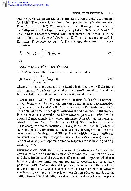
QUASI-ORTHOGONALITY The reconstruction fo~ula is only an approxi-mation from which, by iteration, one can obtain an exact reconstructionoff(x) when C ~ 1 and R ~ 0 (Daubechies et al 1986, Daubechies 1987).This optimal frame is then quasi-orthogonal and complete (tight frame).For instance let us consider the Marr wavelet, O(x) = (1-xZ)e-~/z. Itsoptimal frame, namely that which minimizes R in (30), corresponds A log l = 2~/~ and Ax = 1/2 (Daubechies 1989). With this frame the errorin the energy for the reconstruction off(x) is less than 2 x 10- ~, which sufficient for most applications. The discretization A log l = 2 and Ax = 1corresponds to the dyadic grid (Figure 4a), for which it is also possible construct some exactly orthogonal wavelet bases (Section 4.2). For theMorlet wavelet (23) its optimal frame corresponds to the dyadic grid onlywhen I k¢} = 3.
INTERPOLATION With the discrete wavelet transform we have lost thecovariance by dilation and translation of the continuous wavelet transformand the redundancy of the wavelet coefficients, both properties which canbe very useful for signal analysis and signal processing. It is actuallypossible, under some additional hypotheses, to recompute the whole setof the continuous wavelet coefficients from a discrete subset of the waveletcoefficients by using an appropriate inte~olation (Grossmann & Morlet1984, Grossmann et al 1989) based on the reproducing kernel property
www.annualreviews.org/aronlineAnnual Reviews

418 FARGE
aXmin=0 x=2 J i Xmax=2 J (1-1)
b
Discrete filters associated to scaling functions ~
Analysis
Convolution] the dual the discreteby of
filter associated toscaling functions
Deconvolution] the discreteby
filter associated :oscaling functions
Convolution~ the dual the discreteby of
filter associated to
Deconvolutionthe discreteby
filter associated to
Ovcrsampling by] putting one zero
Undersampling by] taking one sample
] Multiplication by 2
Synthesis
fT.l
FixTure 4 Multiresolution analysis. (a) The dyadic grid, (b) Illustration of the multiresolutionprinciple in Fourier space, (c) Mallat algorithm.
www.annualreviews.org/aronlineAnnual Reviews
WAVELET TRANSFORMS 419
(Section 3.2) of the continuous wavelet transform. With the frames andthe interpolation formula, we now have a complete methodology forextracting the quasi-orthogonal discrete wavelet coefficients from the con-tinuous wavelet coefficients using the wavelet frames and vice-versa torecover the continuous wavelet coefficients by interpolating from the dis-crete wavelet coefficients. This two-way approach allows us to combinethe redundancy and the geometrical properties of the continuous wavelettransform with the economy of the discrete orthogonal wavelet transform.Therefore in practice the distinction between the continuous wavelet trans-form and the orthogonal wavelet transform is often not so important.
4.2 Orthogonal Wavelets
DEFINITION AS we have seen, the frames F are quasi-orthogonal completesets of L2(R). But there also exist some special wavelets ~b such that
~s~i(x) = U/2~s(2~x--0, withj~Z, i~Z, (31)
constitutes a genuine orthogonal basis of Li(R); namely the functions $(x)are orthogonal to their translates by discrete steps x = 2-j’i and theirdilation by l = 2-s, which corresponds to the dyadic grid (Figure 4a), andthe family (31) is complete in L2.
Using an orthogonal wavelet basis {~Oji}, we can decompose any functionor distributionf(x), decaying sufficiently fast at infinity, such that
+oo 4-~o
f( X)= Z Z ~’i~ji(X) (32)j~--m i=--oo
with
~i= <~b,i’f) = f T f(x)~b(x-2-’i)dx’_
Orthogonality implies that the total energy is conserved:
tf(x)12dx = ~ ~ I~-i[2. (33)-- j=--~ i=--~
Contrary to the continuous wavelet transform (Section 3.2) thc orthogonalwavelet transform is not covariant by translation and dilation, except bydiscrete translations 2-Ji and discrete dilations 2-~. To recover in practicethe translational covariance Mallat and Zhong considered the zero-cross-ings, or the local extrcma, of the orthogonal wavelet coe~cicnts, insteadof the coe~cients themselves (Mallat & Zhong 1990, 1991). They haveMso shown that it is possible to have a unique and complete reconstructionof the signal from the local cxtrcma alone, due to the reproducing kernel
www.annualreviews.org/aronlineAnnual Reviews

420 FARGE
property (Section 3.2) of the wavelet transform; however this assertion not true for all functions as Meyer (personal communication) has recentlyproved.
MULTIRESOLUTION ANALYSIS If we want to generalize the wavelet trans-form to decompose any function or distribution j(x) whatever its decayat infinity, we must use, in addition to the analyzing wavelet 0, anotherfunction ~b, called the "wavelets’s father" or "scaling function," such that
f -~ d~(x) dx = 1,
(34)
where
~bj~ = U/2~b(2Jx- i) is orthogonal to 4’j’r forj’ > j and Vi’, (35)
It has been proven (Mallat 1989b) that ~bjk is orthogonal to all its discretetranslates.
Consequently the decomposition off(x) becomes:
f(x)= (Ooilf)c~oi(X)+ ~ (0~i [f)0~,(x). (36)i=--ov j=O i= oo
The first sum is a smooth approximation of f(x) at the largest scale/max = 2o = 1, while the second sum corresponds to the addition of detailsof scale l = 2-~, je[0, + c~]. The function ~0 is a low-pass filter, while ~.jconstitutes a set of orthogonal higher and higher pass filters. Thisapproach, also called multiresolution analysis, is appropriate for analyzingfunctions which are not in LZ(R). Take for example f(x) -= 1, which isnot square integrable (Meyer 1990a). We then have (q~0~[f)= 1
(0~i[f) = 0, from which we reconstruct f(x)= 1; this reconstructionwould have been wrong if we had only used the wavelet ~ without thesmoothing function qS, such as in Equation (32).
The elegance of the multiresolution analysis comes from the fact thatthe scaling functions q~i generate a set of nested subspaces V0 c Vlc ...V~ c V~+l . . . while the associated wavelets 0j~ constitute their ortho-gonal complementary subspaces W0, W~ . . . Wj, W~+~ . . . such thatV~+I = V~ ® W~ (Figure 4b). The inclusion Vj = Vj+ ~ corresponds to mesh refinement by a factor of 2:
f(x)e V~.~ f(Zx)e V~+ (37)
This indicates that the approximation off(x) at scale (~+ I) is
fJ+ I(X) = E ((~(J+ l)/]/)qg~+ (38)
www.annualreviews.org/aronlineAnnual Reviews

WAVELET TRANSFORMS 421
and contains all the necessary information to compute the same signal atthe larger scale 2 J. When computing an approximation off(x) at scale2-j, some informationf is lost, but as the scale decreases to 2 ~ --- 0 theapproximated signal converges to f(x). Conversely, as the scale increasesto l = ~ the approximated signal contains less and less information andconverges to zero.
Vj is the set of all possible approximations at scale l = 2-j of functionsin L2(R). Among all approximated functions at scale ! = -j, f (x) i sthe function that is the closest in L2-norm to f(x). Therefore the waveletdecomposition is an orthogonal projection on the vector space V~.
All the smooth approximations~(x) at scalej off(x) belong to Vj, whileall the additional details~.(x) necessary at scalej to exactly recover~+ ~(x)at scale j+ 1 belongs to W~:
f~+~ (x) = f~(x) +j~(x). (39)
Recursively we obtain the reconstruction formula
f(x) =f0(x)+ Z ~.(x), (40)j=0
which corresponds to the decompositionL2(a) = ° wj.(41)
MAT.~,T AL~Or~TUr~ An additional simplification introduced by Mallat(Mallat 1989a-d) allows the computation of the scaling function q~ froma discrete filter F~, similar to the Quadrature Mirror Filters used in signalcoding (Esteban & Galand 1977, Rioul 1991). This filter 0 comes fromthe space inclusion V0 = V~ which implies
q~(k) =F~ ~ ~ ~ with ~’~(k)-= 2-’/~F4~(Oe,/~ (42)
and therefore recursively for all Vj c V~+ ~,
~(k) = 1-I/0~(2-~k)¯ (43)
The filter ~’~ is 2r~ periodic and satisfies:
f~(0) = 1 to ensure L~-norm normalization,
F~(i --, c~) = (9(i -~) in order for q~ to decay at infinity,
IP~(k)l~÷ IP6(k÷ ~-- 1
in order for/6~ to be a conjugate filter. (44)
www.annualreviews.org/aronlineAnnual Reviews

422 FARGE
The smoothness of the scaling function ~b and its asymptotic decay atinfinity can be estimated from the properties of P~(k).
For instance, we can characterize the Meyer orthogonal wavelets bytheir associated discrete filters:
1
~(k) 0 < fie(k) _<
0
[/~,(k) 12 + 1~(1 - k)12
with
and
if0 _< Ikl -< ~
< Ikl < ~- (45)if~2re
2~iflkl _>-
3
Yk
~(k) =
~(k) + ~(z- k)
~(k) =
if0 < Ikl ~ ~
if~ 2~
2r~iflk[ _>-
3
a(k) = a(- Yk.
Meyer wavelets are very regular (C~) but not very well localized in physicalspace. Their decrease at infinity depends on the smoothness of functiona(k); if a is ~, the associated Meyer wavelet will h ave afast decay. Thereare other orthogonal wavelets, based on spline functions of order m, whichare better localized, with an exponential decay, but which are consequentlyless regular, only Cm- ~; this is the case for instance with the Battle-Lemari~wavelets (Figure 5a).
The Mallat algorithm implies the existence of another discrete filter F~associated with the wavelet ~b and in quadrature with F¢, namely such thatthe filter F, associated with the scaling function q~ is a low-pass filter,while the filter F~ associated with the wavelet ~b is a band-pass filter (Figure4b).
We can then compute the scaling function q~ and its associated wavelet~b from the discrete filter F, alone:
www.annualreviews.org/aronlineAnnual Reviews

WAVELET TRANSFORMS 423
~b(x) = ~F~(i)~(2x-/)i
~(x) = ~ F~(i)~(2x- i
with
F~,(i) = (- 1)~-’F~(1 (46)
In practice, to compute the wavelet transform it is only necessary to knowthe coefficients of the discrete filter F,(0 because, due to the quadraturecondition, F~,(i) is deduced from F,(0 as in Equation (46).
The algorithm (explained in detail in Mallat 1989a, Daubechies 1989,M6neveau 1991 a) then consists of a pyramidal succession of discrete con-volutions of the signal f discretized into I = 2J samples (Figure 4c), firstwith F, to compute the coefficients ~ describing the large-scale behaviorof f up to the scale l = 2-j, and secondly with F, to compute the waveletcoefficients~ describing the behavior of f around the scale l, such as
i’
J~.i = Z F~(i’- 2i)J~._ ,.i,. (47)
This algorithm is pyramidal in the sense that, scale after scale and fromthe small scales to the large scales, we undersample the signal by takingone sample out of every two smaller scale samples; therefore the numberof wavelet coefficients is divided by two at each scale. Finally, due to theorthogonality of the wavelet transform, we obtain the same number I ofwavelet coefficients as the number of samples of the signal. From thosewavelet coefficients f0, ~0 ̄ ¯ ¯ ~, we can then reconstruct a discreteapproximation of the signal at a given scale 2-J, by the same succession ofconvolutions with F~ and Fq,, scale after scale but now going from thelarge scales to the scale 2-.j. Traversing down the pyramid, we must nowoversample the wavelet coefficients by inserting a zero between successivecoefficients, scale after scale. To finally obtain the discrete approximationat scale 2 J’, we add, following Equation (36), both results, f;_ ~ obtainedfrom F~ andj~_ ~ obtained from F~,. For both analysis and reconstructionthe operation count of the Mallat algorithm varies as I log~ L
As for the continuous wavelet transform algorithm (Section 3.3), should beware of boundary effects; these are discussed for instance inM~neveau (1991a). We may also prefer to use periodic orthogonalwavelets, for which a fast algorithm similar to Mallat’s has been developedby Perrier (Perrier & Basdevant 1989), or to use the new orthogonalwavelet bases proposed by Jaffard & Meyer (1989) which vanish on theboundaries, but for which there does not yet exist any fast algorithm.
www.annualreviews.org/aronlineAnnual Reviews

424
OO6
0.8
O.7
O.6
o
(~(x)
0.6
0.2
I0 2tl 30
¢(x)
0
od
04
~(k)
3O
Io 2O 30
Fiyure 5 Examples of scaling functions ~b and associated wavelets ~J commonly used forthe orthogonal wavelet transform. We visualize qS(x), q~(k), ~b(x), and ~(k). (a) Lemari~ wavelet constructed with 4th order spline functions, (b) Daubechies compactlysupported wavelet for N = 2, (c) Daubechies compactly supported wavelet for N =
www.annualreviews.org/aronlineAnnual Reviews

WAVELET TRANSFORMS 425
0.02
-002
o.9F
0.6~
o.~F0.4 !5
0.3
0.2
0
30
~(x)
6 4 2 2
~(k) 60
50
Fi£1ure 5--continued
www.annualreviews.org/aronlineAnnual Reviews
426 FARGE
COMPACTLY SUPPORTED WAVELETS Using Mallat’s procedure (43), Dau-bechies has constructed several compactly supported and regular waveletbases (Daubechies 1988, 1989). She showed that ~b and ~b are compactlysupported if
(2N- 1 )! ~’~ 2N- l[_,g’,(k) 12 = 2 (N_ 1)!22_ sin dx.X (48)
The size of the discrete wavelet support is given by 2N- 1 and depends onthe desired regularity m of the wavelet because N _> m + 1 (Figures 5b,c).
The case N = 1 is the Haar basis which is not regular. But for N # 1we obtain many orthogonal interpolation bases ~bN and their associatedorthogonal wavelet bases $s which are continuous and differentiable untilorder m >_ N/5. For example in the case N = 2 (Figure 5b), the discretefilter which generates the corresponding Daubechies basis is
1 ÷.,/~ 3÷~/~F,~(0)- 4,/~ Fo(1)-
4~
F,(2) -- 3 -- 1 -- ~
4~ F,(3) - 4~ F,(i~]- ~, -- 1] w [4, + m[) = 0.(49)
The numerical implementation of the orthogonal wavelet transfo~ withDaubechies’ wavelets is carried out using the Mallat algorithm. Usingcompactly supported wavelets the operation count, for both analysis andsynthesis, then varies as g which is therefore faster than the Fast FourierTransform.
PERIODIC ORTHOGONAL WAVELETS The extension of the multiresolutionanalysis to the case of periodic wavelets was proposed by Meyer (1986)and performed by Pettier and Basdevant who applied it to build ortho-gonal wavelet bases from periodic spline functions (Pettier & Basdevant1989). The extension of the multiresolution analysis to manifolds such asthe sphere is difficult. For instance the sphere does not have the dilationand rotation invariance of the plane. Recently Jaffard has constructedorthogonal wavelet bases adapted to spherical geometries (Jaffard 1990a,Jaffard & Meyer 1989).
BIORTHOGONAL WAVELETS At first glance Daubechies wavelets lookstrange: They are not symmetric (Figures 5b,c) and for N < 2 theyare left differentiable but not right differentiable (Figure 5b). RecentlyVetterli and Herley have designed some biorthogonal systems of compactly
www.annualreviews.org/aronlineAnnual Reviews
WAVELET TRANSFORMS 427
supported symmetric wavelets built from linear phase filters (Vetterli Herley 1990a-c). The use of biorthogonal wavelets constitutes a newapproach initially proposed in the context of the continuous wavelet trans-form by Tchamitchian (1986, 1987), and then in the context of the ortho-gonal wavelet transform by Cohen, Daubechies, and Feauveau (Feauveau1989, 1990; Cohen et al 1990; Cohen 1990). It replaces the wavelet $ by pair of wavelets, one used for the analysis and the other used for thereconstruction. Biorthogonal wavelets are very promising because theyoffer much more flexibility in the choice of wavelet than orthogonal wave-lets. We can, for instance, choose the properties of both wavelets to becomplementary, with high-order cancellations for the analyzing waveletand good regularity for the synthesizing wavelet.
N-DIMENSIONAL ORTHOGONAL WAVELETS In contrast to the continuouswavelet transform we do not yet know how to compute an orthosonal
wavelet transform using an intrinsically n-dimensional wavelet, but it iscertainly feasible. We are presently left with a partially satisfactorysolution, namely that of separating the orthogonal wavelet transform ofa n-dimensional field into n orthogonal wavelet transforms performed ineach spatial direction. This variable separation approach, which can alsobe used for the continuous wavelet transform, is therefore intrinsicallyanisotropic and requires 2"- 1 wavelets.
For instance, to obtain a two-dimensional multiresolution analysis westart from a one-dimensional multiresolution analysis, defined by the scal-ing function ~b, from which we deduce its associated wavelet $. Then bytensor products we obtain the two-dimensional scaling function
q~(xl, x~) = q~(x0~(x2) (50)and the associated wavelets
I//I(X,, X2)
[//2(Xl, X2)
~0~(x~, x2) This is the approach used to extend the Mallat orthogonal wavelet algo-rithm to two dimensions (Mallat 1988) and to three dimensions (Meneveau1991a).
4.3 Wavelet Packets
Very recently, motivated by data compression problems, Coifman, Meyer,and Wickerhauser have defined and catalogued an extensive "library" of
www.annualreviews.org/aronlineAnnual Reviews
428 FARGE
functions they called "wavelet packets," from which can be built a count-able infinity of orthogonal bases of L2(R) (Coifman et al 1990a,b; Wicker-hauser 1991). The infinitely many bases of wavelet packets unify Gaborwave packets [used in the Windowed Fourier Transform (Gabor 1946)]and wavelets into a set of localized oscillating functions of zero-meanparametrized by scale l, space x, and frequency k: l corresponds to thewidth of their spatial support, x to the position of their center, and k tothe number of oscillations in their spatial support. A wavelet packet familyis thus generated by dilation, translation, and modulation of a "motherwavelet." The different transforms (Figure 1) can be seen as the con-volution of a given signal to be analyzed with a bank of filters given bythe analyzing functions: filters of constant bandwidth Ak for the WindowedFourier Transform or filters of constant ratio of width to center frequencyk for the Wavelet Transform (5). The Wavelet Packets Transform in factcombines these two approaches and offers the possibility to adjust theratio Ak/k of the analyzing functions to the signal to be analyzed.
In the discrete case Coifman and Meyer have derived analytic formulasto generate the 2~ wavelet packets associated with a signal sampled on Ipoints. Their wavelet packets are given as a set of I log21 vectors organizedinto a binary tree, which drastically facilitates further computations. Thenfor a given signal, or for each portion of it after performing an appropriatesegmentation, one can choose the most appropriate orthogonal basis todecompose it. Wickerhauser proposes to select the basis that minimizesthe information entropy or the number of bits necessary to code theinformation content of the signal (Wickerhauser 1991, Coifman et al 1990b).In practice the best basis will be that which minimizes the number ofsignificant (that is above a certain threshold) coefficients. Therefore thewavelet packet transform of a signal of length I gives at most I coefficients(in general many fewer) from which the signal can be resynthesized. Theanalysis requires I log2 I operations and the synthesis I operations. Thewavelet packet decomposition gives orthogonal bases quite similar to thoseobtained with the Karhunen-Lo6ve decomposition, or Proper Ortho-normal decomposition (Lumley 1981, Aubry et al 1988), but its computingcost is much less; indeed the Karhunen-Lo6ve decomposition requiresthe computation of the eigenfunctions of the correlation matrix, whichcontains 13 coefficients.
Torr6sani has proposed a generalization of the wavelet packet transformto the continuous case in which the wavelet packets are indexed by acontinuous parameter (Torr6sani 1991). The wavelet transform in factadapts the tiling of the phase-space (Figure 1) to each portion of thesignal. For instance, in regions dominated by harmonic behavior it willchoose the most appropriate Gabor wave packet basis (Figure 1 e), while
www.annualreviews.org/aronlineAnnual Reviews

WAVELET TRANSFORMS 429
regions with strong transients or shocks it will choose the most appropriatewavelet basis (Figure ld). Another construction which involves waveletpackets with discrete scale parameters and continuous translation pa-rameters has recently been proposed by Duval-Destin et al (1991).
5. WAVELET APPLICATIONS TO TURBULENCE
5.1 Energy Decomposition
A very common pitfall when using any kind of transform is to forget thepresence of the analyzing function in the transformed field, which maylead to severe misinterpretations, the structure of the analyzing functionbeing interpreted as characteristic of the phenomena under study. Toreduce this risk we should choose the analyzing function in accordanceto the intrinsic structure of the field to be analyzed. For instance thetrigonometric functions used in the Fourier transform would be the appro-priate tool if and only if a turbulent flow field were a superposition ofwaves; only in this case are wavenumbers well defined and the Fourierenergy spectrum meaningful for describing and modeling turbulence. If,on the contrary, turbulence were a superposition of point vortices then theFourier spectrum in this case would be meaningless. The problem we stillface in turbulence theory is that we have not yet identified the typical"objects" that compose a turbulent field. Before developing a turbulencemodel we must identify these elementary "objects" and catalog theirelementary interactions. For instance the cascade models (Desnjanski Novikov 1974, Kraichnan 1974, Frisch & Sulem 1975, Bell & Nelkin 1978,Gledzer et al 1981) assume that wavenumber octaves are the elementaryobjects needed to describe homogeneous turbulence and that their inter-actions consist of exchanging energy with the neighboring octaves.
The first step toward modeling turbulence is to find an appropriatesegmentation of the energy density in x- l phase space (Figure 1) and define some kind of phase-space "atoms" among which energy, or anyother dynamically relevant quantity, is distributed and exchanged by theturbulent flow dynamics. If a turbulent field is a superposition of waves,the energy density should be distributed in phase space among horizontalbands, each band corresponding to an excited wavenumber (Figures 2b,c).If a turbulent field is a set of localized structures--often called coherentstructures--the energy density should be distributed among cone-likepatterns, each cone pointing to an excited structure (Figure 2a). If turbulent field is a superposition of wavepackets, such as Tennekes andLumley’s eddies (Tennekes & Lumley 1972), the energy density should distributed among patches whose horizontal length will correspond to the
www.annualreviews.org/aronlineAnnual Reviews

430 rARGE
spatial support and vertical length to the bandwidth characterizing eachexcited wavepacket. If a turbulent field is mainly some kind of noise,its energy density should be randomly distributed in both space andscale without presenting any characteristic pattern in phase space (Figure2c). Actually a turbulent field may well be the superposition of dif-ferent phase-space structures which can be separated into characteristicclasses. In this case it will be more appropriate to decompose the flow fieldinto those classes and then perform separate ensemble or time averages,class by class, in order to retain as much dynamically meaningful infor-mation as possible on the flow. Another solution is to perform the aver-aging directly in phase space, which presents the advantage of being ableto add together experimental data of different signal-to-noise ratios ornumerical fields computed at different resolutions. It also may well bethat different types of turbulence (e.g. boundary layer, mixing layer, gridturbulence...) or different regimes (e.g. transition, fully-developed tur-bulence), will lead to different segmentations of phase space; this shouldbe checked and, if it is the case, we should probably abandon the questfor a universal theory of turbulence.
Finally we should study how the turbulent dynamics transports thesespace-scale "atoms," distorts them, and exchanges their energy during theflow evolution. Using a space-scale representation it would then be easyto verify whether energy transfers are either mainly local in scale--asassumed by the cascade models--corresponding to vertical translations inphase-space, or whether energy transfers are instead local in space--asassumed by point vortex models--corresponding to horizontal trans-lations in phase-space. Energy transfers may in fact be local in both spaceand scale, which is probably the right answer. Wavelets or wavelet packetsare certainly good candidates for performing this energy decompositionin phase space and for finding possible phase-space atoms to characteriz~the turbulent flow dynamics and hence to formulate new turbulencemodels.
5.2 New Diagnostics for Turbulence
Before discussing the actual applications of wavelets to turbulence, let usemphasize two points. First of all, wavelets are useful as a new diagnostictool for the study of turbulence if we want to retain some informationabout the spatial structure of the flow. If we are only interested in itsfrequency content, or if we want to filter it everywhere in space, waveletsare not helpful, and the Fourier transform is a sufficient tool. Secondly,we should always bear in mind the fact that wavelets see signal variationsbut are blind to constant and other global polynomial behavior, accordingto the number of cancellations (Section 3.2) of the analyzing wavelet.
www.annualreviews.org/aronlineAnnual Reviews
WAVELET TRANSFORMS 431
common pitfall in interpreting wavelet coefficients is to link their strengthto the signal’s strength, whereas they actually correspond to variations inthe signal at a given scale and a given point. If the signal does not oscillateat a certain scale and position, then the corresponding wavelet coefficientsare zero.
For the purpose of analysis we prefer to use the continuous wavelettransform whose redundancy allows an unfolding of the flow informationon the space-scale complete grid, as opposed to the dyadic grid used fororthogonal wavelets. As we have already said (Section 3.3), we stronglyadvise using a progressive complex-valued wavelet, because, due to thequadrature between the real and imaginary parts of the wavelet, we canthen eliminate spurious oscillations of the wavelet coefficients by visual-izing their modulus, instead of their real part (Figure 2). If we analyze two-dimensional field using a two-dimensional wavelet we have at least athree-dimensional coefficient space to visualize. If the coefficients are realand therefore oscillate at all scales and locations, their graphical repre-sentation is very complicated and difficult to interpret, whereas the modu-lus only follows the signal energy density variations without presentingspurious oscillations.
The squared wavelet coefficient If(l, x, 0) ]2 measures the energy level, orexcitation, of a given field f(x) in terms of space, scale, and direction. Letus consider the case of three-dimensional turbulence and analyze three-dimensional fields in terms of three space dimensions x -- x, and threeangles 0 = 0,, for n = 1 to 3. By choosing an isotropic wavelet, or averagingover directions, we can discard the angular selectivity of this analysis. Thisis what we shall do from now on in order to simplify the notation. We willnow list several new diagnostics, for two (n = 2) or three (n = 3) dimen-sional turbulence, all based on wavelet coefficients.
LOCAL WAVELET ENERGY SPECTRUM First of all the notion of "localspectrum" is antinomic and paradoxical when we consider the spectrumas a decomposition in terms of wavenumbers for, as we have previouslysaid, they cannot be defined locally. Therefore a "local Fourier spectrum"is nonsensical because, either it is non-Fourier, or it is nonlocal. There isno paradox if instead we think in terms of scales rather than wavenumbers.
Using the wavelet transform, let us define the space-scale energy density:
If(/,x)l2E(I, x) - l" (51)
As proposed by Moret-Bailly et al (1991) in the context of turbulence, thescale decomposition in the vicinity of location x0 is given by
www.annualreviews.org/aronlineAnnual Reviews
432 FARGE
Ez(l, x0) = l 1 n E(l, x)z~j x, (52)
Z being a function of finite support [xl, x2], which takes into account allcoefficients inside the influence cone (Section 3.2) of x0, such that:
fz(x) dnx = (53)
If we choose the window Z to be a Dirac function, then the local waveletenergy spectrum becomes
If(/,x0)l2E~(t, x0) r (54)
By integrating (51) we obtain the local energy density:
fo+~
dlE(x) = C~’+ E(l,x) (55)
GLOBAL WAVELET ENERGY SPECTRUMThe global wavelet spectrum is
Eft) = f~ Eft, ~) d~x. (~6)
It can also be expressed in terms of the Fourier energy spectrumE(k) = If(k)[ 2 using relation (7):
E(l) ~ E(k) l~ (/k)[ 2 d~k. (57)
This shows that the global wavelet energy spectrum corresponds to theFourier energy spectrum smoothed by the wavelet spectrum at each scale.
We can then recover the total energy of the fieldf(x):
~ = C;~ ~(07.
LOCAL INTERMITTENCY ~AS~E To measure intermittency, namely thefact that energy at a given scale may not be evenly distributed in space,Farge et al (1990) have defined the intermittency measure:
If(/,x)]2~(~, x) = (If(l, x) (59)
I(l, x) = 1, Vx and Vl, means that there is no flow intermittency, i.e. that
www.annualreviews.org/aronlineAnnual Reviews

WAVELET TRANSFORMS 433
each location has the same energy spectrum, which then corresponds tothe Fourier energy spectrum. I(l, x0) -- 10 means that the point x0 con-tributes 10 times more than the average over x to the Fourier energyspectrum at scale I.
Frick & Mikishev (1990) had previously defined a similar intermittencymeasure using the Zimin hierarchical model (Zimin 1981).
SPACE-SCALE REYNOLDS NUMBER AND GLOBAL INTERMITTENCY MEASURE
Farge et al (1990b) have introduced a space-scale Reynolds number
~(l, x) Re (l, x) , (60)
where v is the kinematic viscosity of the fluid and g the characteristic rmsvelocity at scale l and location x such as:
f(l,x) = (3C0)-I ~ [~7,(l,x)[ 2 . (61)
At large scales 1 ~ L,
.Re (L) = Re (L, x) co
coincides with the usual large-scale Reynolds number Re = v’L/v, wherev" is the rms turbulent velocity and L the integral scale of the flow. At theKolmogorov scale l ~ r/, where dissipation effects equilibrate nonlineareffects, Re(r/, x)= 1. In plotting the iso-surface Ref/,x)= 1 we can thencheck whether it is fiat or not. If it is flat, then 1 = r/ everywhere, asassumed by Kolmogorov’s theory. If it is not flat, then the turbulent flow isintermittent and we can no longer define a unique Kolmogorov scalebut only a range of scales from r/rain to r/~-~x" The ratio /(Re) = r/max/r/rain,
for Re = 1, is a global measure of the flow intermittency in the dissipativerange. The ratio/(Re) lmax(Re)/lmin(Re), for Re>> 1, measures theglobalflow intermittency in the inertial range.
For direct numerical simulations of turbulent flow, this iso-surfaceRe(l, x) = 1 may be useful in detecting numerical errors and verifying the space resolution Ax is sufficient to resolve the dissipative scales every-where in the flow. We have to verify that r/rain > AX everywhere in the flow,otherwise for points where this inequality is not verified some numericalinstability may develop.
For numerical simulations we can define a better space-scale Reynoldsnumber. For this we must compute the nonlinear term N = II v o Vv II and
www.annualreviews.org/aronlineAnnual Reviews

434 FARGE
the dissipative term D = ]] v" V2v][ and expand them into their waveletcoefficients to obtain
Re(l, x) =/~(l, x)//~(l, (62)
SPACE-SCALE CONTRAST If we want to detect any variation in the signal,even for regions where the signal becomes very weak, Duval-Destin andTorrrsani (Duval-Destin & Menu 1989; Antoine et al 1990, 1991; Duval-Destin et al 1991; Antoine & Duval-Destin 1991) have proposed thecontrast measure
cq, x) If(t,- If(l, x) 2’ (63)
with
f(l,x) = ~l/-(n+l) f(l’,x)dl’.dl,=0+
For orthogonal wavelets the contrast has the very elegant form
(64)
~Oji being the orthogonal wavelets, at scale j and location i, and ~bji theassociated scaling functions.
While wavelet coefficients locally measure the signal derivative, thespace-scale contrast measures its logarithmic derivative. This diagnosticmay be useful in fluid mechanics for detecting some very weak coherentstructures, or some coherent structures embedded in larger ones--twocases that cannot be detected by the classical threshold method. In anycase wavelets are better adapted to filtering or segmenting flow fields thantraditional image processing techniques; most image processing techniquesare based on contour detection developed for pattern recognition, whereascoherent structures encountered in fluid flows do not have sharp contoursbut instead are characterized by their local scaling. A similar problem isencountered in analyzing astronomical images, in particular in detectinggalaxies, for which wavelets are now extensively used (Bijaoui 1991).
SPACE-SCALE ANISOTROPY MEASURE The measure of the space-scale depar-ture from isotropy is given by
www.annualreviews.org/aronlineAnnual Reviews

WAVELET TRANSFORMS 435
A(l, 0) = + ~o " (65)
For this diagnostic we obviously must use a directional wavelet such asthe Morlet wavelet (Section 3.3).
If A(l,O) = 1, ¥l and ~’0, the flow is isotropic at all scales.If A(/min, 0) A(lma,, 0), V0, with/min a small scale and lmax a large scale,
there is a return to isotropy in the small scales.A(l, ~o) 10means that dir ection ~0 contributes 10 times more than the
average over 0 to the Fourier energy spectrum at scale l.
LOCAL SCALING AND SINGULARITY SPECTRUM As we have said in Section3.2, the continuous wavelet transform with L~-norm (19) is used to studythe local scaling of a function and to detect its possible singularities. Butto see singularities, we must subtract the Taylor series of the signal, whichcorresponds to its polynomial, and therefore differentiable, terms. Thissubtraction is automatic if we choose a wavelet with sufficiently manycancellations (Section 2.2 and 3.1) to be blind to these polynomial con-tributions. Here again a complex-valued wavelet is preferable. To justifythis choice, let us take as a counterexample the analysis of a singularityIx-x01~, 0 < ~ < 1, located at x0, using a real-valued wavelet. If thesingularity is odd and the wavelet even, or vice-versa, then the small-scalewavelet coefficients will be zero at x0 and we will not see the singularity,for it has been cancelled by the signal’s, or wavelet’s, zero-crossings. If wechoose a progressive complex-valued wavelet, whether odd or even, theL L-modulus of the wavelet coefficients will drastically increase in the smallscales around the location x0 and the rate of increase will give the exponentof the singularity. The local scaling off(x) at x0 is given by the scaling the wavelet coefficients’ Lt-modulus in x0 in the limit of asymptoticallysmall scales, l -~ 0. This property has been used by Tchamitchian & Hol-schneider (1989, 1990) to study the local regularity of the Riemann func-tion: they have demonstrated that the Riemann function is differentiableon a dense set of points and is singular everywhere else.
To compute the singularity spectrum, we should proceed as follows.First, we plot the phase of the wavelet coefficients to locate singularities--for the iso-phase lines will point towards singular points. Second, weshould verify that the singular point detected at x0 is isolated, namely that
f(l ~ 0, x0) < f(l -~ 0, x0 + a), with l al very small. (66)
www.annualreviews.org/aronlineAnnual Reviews
436 rAaoE
Then the exponent ~(x0) of the singularity is given by the slope of the localscaling of log If(l, x0)l for l-~ 0, f being written in Lt-norm (19). singularity spectrum has been used tO characterize fractal and multi-fractalmeasures (Arn6odo et al 1988, 1989; Arn6odo et al 1990; Arn6odo et al1991), and its generalization to fractal and multi-fractal functions has beenrecently made by Muzy et al (1991). Using a real-valued wavelet, Bacry al (1991) first extract the wavelet coefficients "skeleton," i.e. the locationof the local maxima of the wavelet coefficients, before computing the localscaling. Benzi & Vergassola (1991) proposed a procedure, called "theoptimal wavelet transform," to reduce possible oscillations of If(l, x0)lversus log 1 while using a real-valued wavelet. This procedure is com-putationally intensive and has been recently improved by using a pro-gressive complex-valued wavelet (Morlet) instead of a real-valued one(Benzi & Vergassola 1991).
5.3 Some Preliminary Results Usint7 Wavelets
voR Tt~RBt~LEr~¢~ ANALYSIS Wavelet analysis of turbulent flows is atpresent developing rapidly in many different directions. As a consequence,! cannot detail and discuss all published papers on this subject, thus willonly list those I know of, so that the reader may have access to them.As noted in the introduction, most of these papers have an exploratorycharacter and their conclusions may not yet be definitive. They do havethe merit of clarifying the concepts inherited from the Fourier spectralapproach, of asking new questions, and of introducing new points of viewconcerning our understanding of turbulence.
To my knowledge, the wavelet transform was first used in fluid mech-anics by Saracco and Tchamitchian in a study of the propagation oftransient acoustic signals in inhomogeneous media (Saracco & Tcha-mitchian 1988, Saracco et al 1989). In the context of turbulence, waveletswere first used by Farge and Rabreau to analyze two-dimensional homo-geneous turbulent flows obtained from numerical simulations, using firsta one-dimensional Morlet wavelet (Farge & Rabreau 1988a,b; Farge Sadourny 1989) and then a two-dimensional Morlet wavelet (Farge Holschneider 1989, Farge et al 1990a, Farge 1990). They showed thatduring the flow evolution, starting from a random distribution of vorticitywith a k- 3 energy spectrum, the small scales of the vorticity field becomeincreasingly localized in physical space (Figure 6). This suggested an inter-mittency of the two-dimensional turbulence dynamics, which may berelated to a condensation of the vorticity field into vortex-like coherentstructures. In particular they found that the smallest scales of the vorticityfield are concentrated inside some vortex cores (Figures 7, 8) and aregenerated when and where two same-sign coherent structures are merging
www.annualreviews.org/aronlineAnnual Reviews
438 FARCE
(Farge et a 9 9 0 a ) . From this observation, Farge and Holschneider pro- posed a new, purely geometrical, interpretation of the k4 cnergy spectrum observed for numerically computed two-dimensional turbulent flows, based on the existence of cusp-like axisymmetric coherent structures with a scaling exponent of -1/2 (Farge & Holschneider 1991). Such quasi- singular coherent structures are scaling distributions of vorticity which exhibit, instead of a characteristic radius, a range of radii corresponding to all scales of the inertial range, until the dissipative scales where the vortex cores are smoothed. These cusp-like coherent structures are also characterized by a nonlinear pointwise relation between vorticity and streamfunction, similar to coherent structures experimentally observed in a two-dimensional turbulent mercury flow (Nguyen Duc & Sommeria 1988). Farge and Holschneider have conjectured that those quasi-singular vortices are created by the condensation of the vorticity field around quasi- singularities already present in the initial conditions (Farge & Holschneider 1991). They have also shown that coherent structures with a scaling exponent of - 1/2 are stable under the two-dimensional Navier-Stokes dynamics, even when perturbed by strong noise, and these structures organize the random field in their vicinity by accreting the same-sign noise onto them (Farge et a1 1991a). Recently Benzi and Vergassola, by performing a wavelet analysis of a numerically computed two-dimensional homogeneous turbulent flow, have confirmed the existence of coherent structures with negative exponents, between -0.4 and -0.6, similar to the -0.5 scaling exponent predicted by Farge and Holschneider (Benzi & Vergassola 1991).
The first wavelet analysis of an experimental turbulent signal was carried out by Argoul et al from the wind tunnel streamwise velocity measured at high Reynolds by Gagne and Hopfinger, using one-dimensional real- valued wavelets (Argoul et a1 1989, Arntodo et a1 1990, Bacry et a1 1991, Arnkodo et a1 1991). At about the same time, Liandrat, Moret-Bailly, and Tchamitchian, using a one-dimensional real-valued wavelet, studied the interaction between a shock wave and free turbulence, and then analyzed the streamwise velocity in a turbulent boundary layer near a heated wall
L
Figure 7 Two-dimensional continuous wavelet transform computed in the L'-norm, using the real-valued DOG (Difference of Gaussians) wavelet. The same two-dimensional turbulent flow (vorticity field sampled at 512' points) as in Figure 6 for n = IOs has been used. We visualize the wavelet coefficients (fefi) at: scale I = 8 A x (top), scale I = 4 A x (middle), scale 1 = 2 A x (bottom); where A x is the mesh size. We then visualize the partial reconstructions of the vorticity field (right) from the wavelet coefficients, taking all coefficients up until: scale I = 8 A x (top), scale I = 4 A x (middle), scale I = 2 A x (bottom).
www.annualreviews.org/aronlineAnnual Reviews

WAVELET TRANSFORMS 439
www.annualreviews.org/aronlineAnnual Reviews

440 PARGE
%?Kre 8 Two-dimensional continuous wavelet transform computed in the L'-norm, using the complex-valued Morlet wavelct with (k,l = 5 and 0 = 0, of the same two-dimensional turbulent flow (vorticity field sampled on 512' points) as Figure 7. The black and white f igus illustrates the vorticity field to be analyzed. The color plate shows the wavelet coefficient modulus (color coded in the increasing order: blue, red, magenta, green, cyan, yellow, and W h i W and phase (.qru,v ixu/;tw.y) mapped onto the vorticity field (in perspective representdon) at: scale I = 32 Ax (lop) and scale 1 = 16 Ax (botrom). (From Farge et a1 1990a.)
in order to compare both wavelet and VITA (Variable Interval Time Averaging) techniques (Liandrat & Moret-Bailly 1990). They also used the wavelet transform to estimate the transition Reynolds number in a rotating disk boundary layer (Moret-BaiIIy et a1 1991). More recently Frisch and Vergassola have proposed a new type of averaging for turbulence analysis, namely a scale-averaging of the logarithm of the wavelet coefficients modu- lus, which, like time-averaging of stationary processes, reduces statistical fluctuations of self-similar random processes, provided there is a sufficient range of scales in the signal (Vergassola & Frisch 1990). In the study of stochastic processes and multiscale statistical signal processing, many developments are presently underway (Basseville & Benveniste 1989, 1990;
www.annualreviews.org/aronlineAnnual Reviews
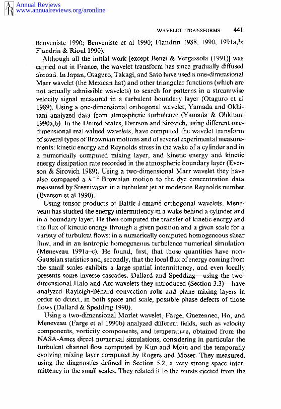
WAVELET TRANSFORMS 441
Benveniste 1990; Benveniste et al 1990; Flandrin 1988, 1990, 1991a,b;Flandrin & Rioul 1990).
Although all the initial work [except Benzi & Vergassola (1991)] wascarried out in France, the wavelet transform has since gradually diffusedabroad. In Japan, Otaguro, Takagi, and Sato have used a one-dimensionalMarr wavelet (the Mexican hat) and other triangular functions (which not actually admissible wavelets) to search for patterns in a streamwisevelocity signal measured in a turbulent boundary layer (Otaguro et al1989). Using a one-dimensional orthogonal wavelet, Yamada and Okhi-tani analyzed data from atmospheric turbulence (Yamada & Ohkitani1990a,b). In the United States, Everson and Sirovich, using different one-dimensional real-valued wavelets, have computed the wavelet transformof several types of Brownian motions and of several experimental measure-ments: kinetic energy and Reynolds stress in the wake of a cylinder and ina numerically computed mixing layer, and kinetic energy and kineticenergy dissipation rate recorded in the atmospheric boundary layer (Ever-son & Sirovich 1989). Using a two-dimensional Marr wavelet they havealso compared a k-z Brownian motion to the dye concentration datameasured by Sreenivasan in a turbulent jet at moderate Reynolds number(Everson et al 1990).
Using tensor products of Battle-Lemari6 orthogonal wavelets, Mene-veau has studied the energy intermittency in a wake behind a cylinder andin a boundary layer. He then computed the transfer of kinetic energy andthe flux of kinetic energy through a given position and a given scale for avariety of turbulent flows: in a numerically computed homogeneous shearflow, and in an isotropic homogeneous turbulence numerical simulation(Meneveau 1991a--c). He found, first, that those quantities have non-Gaussian statistics and, secondly, that the local flux of energy coming fromthe small scales exhibits a large spatial intermittency, and even locallypresents some inverse cascades. Dallard and Spedding--using the two-dimensional Halo and Arc wavelets they introduced (Section 3.3)--haveanalyzed Rayleigh-Brnard convection rolls and plane mixing layers inorder to detect, in both space and scale, possible phase defects of thoseflows (Dallard & Spedding 1990).
Using a two-dimensional Morlet wavelet, Farge, Guezennec, Ho, andMeneveau (Farge et al 1990b) analyzed different fields, such as velocitycomponents, vorticity components, and temperature, obtained from theNASA-Ames direct numerical simulations, considering in particular theturbulent channel flow computed by Kim and Moin and the temporallyevolving mixing layer computed by Rogers and Moser. They measured,using the diagnostics defined in Section 5.2, a very strong space inter-mittency in the small scales. They related it to the bursts ejected from the
www.annualreviews.org/aronlineAnnual Reviews
442 FARGE
boundary layer of the channel flow and to the ribs (streamwise vortextubes) stretched and engulfed into the spanwise vortex cores in the case ofthe mixing layer. Extrapolating the local scalings they found, and con-sidering their strong variance from the Fourier spectrum, they conjecturedthat the larger the Reynolds number the larger the degree of intermittency.They have also observed a return to isotropy in the small scales for themixing layer, but not for the plane channel flow whose small scales remainelongated in the streamwise direction. Finally, they found that the iso-Reynolds manifold represented in space and scale (see Section 5.2) is notflat, but presents peaks in the most unstable regions, particularly in thespanwise vortex cores of the mixing layer.
Farge et al (Farge 1991c, Farge et al 1991c) have shown that the waveletpacket bases are much more efficient than the Fourier basis to compresstwo-dimensional turbulent flows. They define the "best basis" as the onewhich condenses the L2-norm (energy or enstrophy) into a minimumnumber of non-negligible wavelet packet coefficients. They have foundthat the most significant coefficients of the best basis correspond to thecoherent structures, while the weakest coefficients, which can then bediscarded, correspond to the vorticity filaments (Figure 9). They havethen performed several numerical integrations initialized, either with anoncompressed vorticity field (reference history), either with a vorticityfield compressed using the Fourier basis, or with a vorticity field com-pressed using the best basis. For a compression ratio 1/2, done in the bestbasis, the time evolution during 6000 time steps of the vorticity fieldremains similar to the reference history, while if the compression ratio isdone in the Fourier basis, the deterministic predictability is lost and onlythe spectral behavior remains similar. Then for compression ratios up to1/200, done in the best basis, the deterministic predictability is lost but notthe statistical predictability, whereas the compression operated in Fourierloses both. This confirms the fact, predicted among others by Farge (1990),that the dynamically active entities of a two-dimensional turbulent floware the coherent structures, while the vorticity filaments are only passivelyadvected by them. Using the wavelet packet best basis the flow separationinto active versus passive components, or "master" versus "slave" modes,is performed without assuming any hypothetical scale separation, as isnecessary when using the Fourier basis. In conclusion, the wavelet packetbest basis seems to distinguish the low-dimensional dynamically activepart of the flow (the coherent structures) from the high-dimensional passivecomponents (the vorticity filaments), which can then be neglected or para-metrized. This gives us some hope of drastically reducing the number ofdegrees of freedom necessary to compute two-dimensional turbulent flows.
To conclude this section on turbulence analysis using wavelets, I would
www.annualreviews.org/aronlineAnnual Reviews
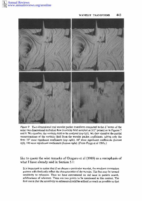
WAVELET TRANSFORMS 443
Figure 9 Two-dimensional real wavelet packet transform computed in the L'-nom of the same two-dimensional turbulent flow (vorticity field sampled at 512' points) as in Figures 7 and 8. We visualize: the vorticity field to be analyzed (top feft). We then visualize the partial reconstructions of the vorticity field from the wavelet packet coefficients, taking only the first: 10" most significant coefficients (top right), lo3 most significant coefficients (bottom kfr), 100 most significant coefficients (bottom right). (From Farge et a1 1991c.)
like to quote the wise remarks of Otaguro et a1 (1989) as a reemphasis of what 1 have already said in Section 5.1 :
It is important to notice that if we choose a particular wavelet, the resultant correlation pattern will obediently reflect the characteristics of the wavelet. The fact may be termed sensitivity to reference. Thus we have encountered an old issue in pattern search, arbitrariness of reference. There are two points to be mentioned in this context. The first one is that the sensitivity to reference should be utilized as much as possible so that
www.annualreviews.org/aronlineAnnual Reviews

444 FARGE
we can search any object in a chaotic field. The second one, which can be contradictoryto the first, however, is that we have chances to capture ghost patterns with no physicalsignificance. This danger has been repeatedly mentioned by many authors. The problemis deeply related to our a priori knowledge about the turbulent field under test.
FOR TURBULENCE MODELING The goal of turbulence modeling using wave-lets is to directly compute the time evolution of a turbulent flow in termsof wavelet coefficients, instead &space variables. If the turbulent dynamicsis governed by some nonlinear cascades, then we should study them inboth space and scale, without assuming, for instance, any scale localityof the transfers as is done for the so-called cascade turbulence models(Desnjanski & Novikov 1974, Kraichnan 1974, Frisch & Sulem 1975, Bell& Nelkin 1978, Gledzer et al 1981, Qian 1988). After writing Euler orNavier-Stokes equations in wavelet space, the problem is then to definethe graph of possible interactions, to estimate their propagation speed inphase space, and to ascertain if transfers are mainly local in space--corresponding to horizontal shifts in phase space, local in scale--cor-responding to vertical shifts, or local in both--if shifts operate alongdiagonals. In studying the symmetries of the Euler or Navier-Stokes equa-tions, and perhaps some variational principles, we might then learn whichkind of interactions dominate and which are forbidden. With this approachto the modeling of turbulence, no statistical hypotheses are needed becausewe directly study a set of algebraic equations obtained by projectingNavier-Stokes or Euler equations onto an appropriate orthogonal basis.In this case the whole endeavor will consist of truncating as much aspossible the number of algebraic equations retained in the turbulence
¯ model. As a first step in this direction, Meneveau (1991c) derived the three-dimensional Navier-Stokes equation in wavelet space. His paper actuallyfocuses on turbulence analysis (see previous paragraph), but he mentionsthat further developments of this formulation should concentrate on pos-sible approximations to the interaction kernel, similar to the work ofNakano (1988) who used a wave packet formulation.
In the same spirit (but before the wavelet theory of Morlet-Grossmann-Meyer) extremely impressive work was carried out by Zimin starting in1981 in Perm, Soviet Union (Zimin 1981). In his first paper, he projectedthe three-dimensional Navier-Stokes equation onto a quasi-orthogonalbasis using functions that were localized in both space and scale. Toconstruct his basis he considered a hierarchy of eddies and assumed thatthe small eddies were advected by the larger ones. This led him to segmentthe phase space into cells of constant size corresponding to eddies whosespatial support decreased with the scale, each eddy having a space-scaleresolution in accordance to the uncertainty principle. In fact the phase-space segmentation of Zimin’s hierarchical basis is the same as for wavelets
www.annualreviews.org/aronlineAnnual Reviews
WAVELET TRANSFORMS 445
(Figure ld). After constructing hierarchical bases for three-, two-, andone-dimensional flows (Zimin 1981, Frick 1983, Zimin et al 1986, Zimin& Frick 1988, Frick & Zimin 1991), Zimin is presently generalizing themto three dimensions plus time (Zimin 1990a,b) in order to be able compute the Navier-Stokes equation in a purely algebraic fashion. Since1981 Zimin’s approach has been extensively used in more than 40 papers--unfortunately most of them have not yet been translated from Russian.Here I only briefly list some of those, translated into English, which usethe hierarchical basis for modeling or computing different types of tur-bulent flows: two-dimensional flows (Frick 1983, Aristov et al 1989, Miki-shev & Frick 1990), two-dimensional MHD flows (Frick 1984, Mikishev& Frick 1989, Aristov & Frick 1990), rotating shallow-water flows (Aristov& Frick 1988a, Aristov et al 1989), and different convective flows (Frick1986a,b; Frick 1987; Aristov & Frick 1988b, 1989).
We should also mention a recent model of turbulence intermittency(Farge & Holschneider 1991, Farge 1991b), differing from previous models(Kolmogorov 1961, Mandelbrot 1974, Frisch et al 1978, Benzi et al 1984,Parisi & Frisch 1985), which all refer to hypothetical stochastic processesand often involve, for instance, eddy breaking. This new model proposesa purely geometrical interpretation of intermittency: spatial intermittency,for both two-dimensional and three-dimensional turbulent flows, may berelated to the quasi-singular shape of a few highly excited axisymmetriccoherent structures, which are produced by the flow dynamics. Due totheir cusp-like shape, these coherent structures do not have a characteristicscale but instead present a range of scales. Moreover, their spatial supportdecreases with scale and follows a power-law behavior before reaching thedissipative scales where their cores are locally regularized by dissipation.The spatial intermittency may then be explained by the geometry of thosecusp-like coherent structures. In addition Farge (1991b) supposes thateach coherent structure may have a different scaling law and may beginto be dissipated at a different scale than the others, which would thereforecorrespond to the different peaks observed on the dissipative manifoldRe(l, x) = 1 (see Farge et al 1990b). This conjecture seems consistent Castaing’s theory of turbulence (Castaing 1989, Castaing et al 1990),which, contrary to Kolmogorov’s theory, assumes a possible weak dis-sipation in the inertial range. It is also consistant with Frisch and Ver-gassola’s multifractal model of a possible intermediate dissipative range(Frisch & Vergassola 1990). It may be that this geometrical interpretationof space intermittency, deduced from the wavelet analysis of two- andthree-dimensional turbulent flows (Farge & Rabreau 1988b, Farge et al1990a,b) is wrong, resulting again from confusion between the scalingproperties of the wavelet family and those of the turbulent field. As I have
www.annualreviews.org/aronlineAnnual Reviews
446 FARGE
previously said (Section 5.1), this is the most common pitfall encounteredwith wavelets and we are not yet immunized against it.
FOR TURBULENCE COMPUTING The objective is to be able to reduce thenumber of degrees of freedom necessary to compute the flow evolution,in order to simulate high Reynolds number flows. As we said in Section1, for Fourier spectral methods (Galerkin or pseudo-spectral) the numberof degrees of freedom varies as Re in dimension two and Re9/4 in dimen-sion three; the direct numerical simulations, i.e. without any ad hoc subgridscale parametrization, are in this case limited to low Reynolds numberflows, even with the fastest supercomputers available today. Fourier spec-tral methods are very precise if the flow remains regular. However, theyare no longer appropriate when the flow develops shocks or steep gradientsbecause solutions will then present some spurious oscillations everywherein the domain (Gibbs’ phenomenon). In this case we prefer to use finiteelement methods, or finite differences which may be thought as a particularcase of finite element methods. In fact, wavelet bases are intermediatebetween finite element bases (due to their space localization) and Fourierbases (due to their scale localization). Now the point will be to use waveletsto develop new numerical techniques which will combine the advantagesof both methods, while avoiding their inconveniences. Numerical methodsusing wavelets are presently in a nascent state, but seem very promising inthe long term. For instance, in the case of partial differential equations,only Burger’s equation in one dimension has been solved using waveletsin two different ways, a wavelet Galerkin method and also a waveletparticle technique.
To illustrate the principle of the wavelet Galerkin method, let us considerthe one-dimensional evolution equation
(67)Lu(x, t = O) = Uo(X),
with A as a differential operator. We can project (70) onto an appropriatemultiresolution space l/" yielding
(I~ + A(u’)l ~b/=0, (68)
with ~ either the scaling function (Latto & Tenebaum 1990, Glowinski etal 1990) or the wavelet associated to the chosen multiresolution (Liandratet al 1989, 1991; Liandrat & Tchamitchian 1990; Maday et al 1990; Pettier1989, 1991a). For a multiresolution based on the discrete filter /~(k)
www.annualreviews.org/aronlineAnnual Reviews

WAVELET TRANSFORMS 447
(Section 4.2), the differentiation becomes very easy if we introduce a secondfilter ~(k) which is the derivative of the first one, as proposed by Lemari~(Perrier 1991b). The only problems arise from the nonlinear operators,which presently must be computed in physical space at each time step, asis done for pseudo-spectral methods. In the case of v’ Vv--the nonlinearoperator so important for turbulence--we can almost compute it directlyin wavelet space (Beylkin 1991). The advantage of a wavelet Galerkinmethod, compared to Fourier, is that it uses the lacunarity of the waveletseries and discards the wavelet coefficients below a certain threshold.Depending on the problem, we can then drastically reduce the number ofdegrees of freedom to compute. For instance, in the case of the one-dimensional Burger’s equation with a weak dissipation, Perrier has shownthat 164 wavelet coefficients are sufficient to achieve the same precision ofthe solution, e = 10-6, as with 1024 Fourier modes (Maday et al 1991;Perrier 1991a,b). In addition, she observes no Gibbs’ phenomenon in thevelocity field away from the shock, as is the case with the Fourier Galerkinmethod.
As we said in Section 5.1, turbulent flows may be thought of as asuperposition of point vortices. This is the basic assumption of vortexnumerical methods which is used for computing turbulent flows (Leonard1985). In this case the solution is approximated as a finite sum of regu-larized Dirac masses, which evolve in amplitude and position. The sameidea is behind the wavelet particle method, but in addition it allows theelementary vortices, substituted for the Dirac masses, to be deformed andtherefore also to evolve in scale. The principle of the wavelet particlemethod (Basdevant et al 1990) is to look for an approximate solution Equation (67), considered as a sum of a given number N of wavelet particlesq~n, or wavelet atoms, which evolve in phase space according to:
tn~-lUn(t)~X--Xn(t)N
U(X, t) l.(t) - ~" V.(x, t).,= 1 (69)
kv.--with l. > 0 and u., x. e R.
The double localization of waxielets in both space and scale ensures theindependence, in the L2 sense, of two wavelet particles ~. and ~m distantenough in phase-space, namely for
l,._l >>0 and ~>>1. (70)
Therefore the time evolution of the solution of Equation (67) will cor-
www.annualreviews.org/aronlineAnnual Reviews

448 FARGE
respond to the trajectories of the wavelet particles in phase space. Inregions where the solution is smooth there will be very few waveletparticles, whereas they will concentrate dynamically in regions where thesolution may become singular. The wavelet particle method (also called"ondelettes mobiles") consists, for each time step, of finding the set of{U ...... u,, l~ ..... l,, Xl ..... x,} that minimizes the local residual fromEquation (67), where
(71)
We must therefore solve a linear system of 3N equations for Oun/Ot, Ol,/Ot,and Ox,/Ot, which is well conditioned only if the different wavelet particlesremain sufficiently separated, How to handle wavelet-particle collisions isstill an open problem; some tentative solutions are discussed in Perrier(1991a).
It is well-known that the importance of Fourier bases stems from thefact that they diagonalize differential operators. Although such operatorslose this very simple form in a wavelet basis, due to the different frequenciesinvolved in the wavelet and required by its space localization, they have amatrix realization that is almost diagonal (Meyer 1990a, Jaffard 1991d).Beylkin, Coifman, and Rokhlin have developed a very efficient algorithm,based on wavelets, which allows one to multiply a matrix by a vector veryefficiently. Thus this algorithm is useful for diagonalizing or invertingcertain classes of dense matrices, and is particularly appropriate to thecase of integral operators (Beylkin et al 1991a). It uses the fact that waveletcoefficients decay rapidly in regions where the function is regular; afterprojecting ~ onto an orthogonal wavelet basis and reordering the terms,the BCR algorithm transforms ~¢ into a band matrix. For instance tosolve Y = ~¢X, to accuracy e, requires only C(e)" operations, wi th Cbeing a constant depending on the precision desired. This algorithm hasbeen used to invert dense matrices of more than 212 elements, whichwould have been impossible in practice with any other method. Othernew algorithms, also based on wavelets, are presently being studied forinverting elliptic operators (Tchamitchia’n 1989a,b; Jaffard 1990b).
All these numerical methods based on wavelets are in a very preliminaryphase and not yet ready to compute the Navier-Stokes or Euler equations.But, as a first step, we can still numerically solve these equations withother, more classical, algorithms and use wavelets only to locally filter thesolutions or detect the strong gradient regions (such as shocks) in orderto remesh the domain when and where it is necessary. Wavelets may alsobe used to define some new ways of forcing the flow field, for instance to
www.annualreviews.org/aronlineAnnual Reviews

WAVELET TRANSFORMS 449
excite only a given coherent structure and not the whole domain as withFourier mode forcing. Finally, we can foresee using wavelets to developnew variants of the Large Eddy Simulation techniques, where the scaleseparation will no longer be defined in terms of Fourier wavenumbers, butwill be based on a separation between coherent structures (i.e. very excitedregions of wavelet phase space) which will be explicitly computed, whilethe background flow (i.e. regions of weak wavelet coefficients) will only globally parameterized using some ad hoc model.
CONCLUSION
The present position of the founders of the wavelet theory--Morlet,Grossmann and Meyer--is to control tlae enthusiasm of the newcomers,who may overestimate the actual possibilities of the wavelet transform andthen create some backlash effect resulting from their disappointment. Myown view is that the wavelet transform is a very young technique which isevolving at a very fast pace, and we therefore must first become accustomedwith it by performing extensive tests on well-known "academic signals" inorder to develop a feeling for it before defining applications for which itwill be useful.
We should also define some appropriate representations of the waveletspace, which is then critical for the two- and three-dimensional wavelettransform. We should develop a feel for the interpretation of waveletcoefficients, in particular for better understanding of the meanings of themodulus and phase in the case of complex-valued wavelets. In addition,we should test many different wavelets to try to optimize the choice ofwavelet for a given problem. We should also find faster continuous wavelettransform algorithms. In the context of turbulence, the wavelet transformcertainly opens some new possibilities, but we should not rely on it to solvethe problem by chance, lest we run the risk--as has already been thecase in this field--of misinterpreting the results by mistaking the scalingbehavior of the wavelet transform for the signal scaling. The wavelettransform is a sophisticated tool and its use might be very fruitful forthe understanding of turbulence, if one is wise enough to first becomeaccustomed with it.
To conclude I quote Yves Meyer (Meyer 1990c):
Wavelets are fashionable and therefore excite curiosity and irritation. It is amazing thatwavelets have appeared, almost simultaneously in the beginning of the 80’s, as analternative to traditional Fourier analysis, in domains as diverse as speech analysisand synthesis, signal coding for telecommunications, (low-level) information extractionprocess performed by the retinian system, fully-developed turbulence analysis, renor-realization in quantum field theory, functional spaces interpolation theory .... But this
www.annualreviews.org/aronlineAnnual Reviews

450 FARGE
pretention for pluridisciplinarity can only be irritating, as are all "great syntheses" whichallow one to understand and explain everything. Will wavelets soon join "catastrophetheory" or "fractals" in the bazaar of all-purpose systems? It seems to me that "wavelets"have a slightly different position, since they do not constitute a theory but rather a newscientific tool. Indeed, they have never been used to explain anything. When M. Fargeuses them to analyze turbulence simulation results, they play nearly the same role as thepair of glasses I use to read the "Apologie de Raimond Sebond." These glasses, nowrequired by my age, should not be condemned if I do not understand Montaigne’sthoughts, or glorified if I admire them. Likewise with wavelets whose modest, butessential, role is to help us to better study, at different scales, complex phenomena.
ACKNOWLEDGMENTS
The wavelet transform examples which illustrate this paper have beencomputed on the Cray-2 of the Centre de Calcul Vectoriel pour laRecherche, Palaiseau, and on other systems, in collaboration with Jean-Frangois Colonna, Marc Duval-Destin, Eric Goirand, Philippe Guille-main, Matthias Holschneider, Gabriel Rabreau, and Victor Wicker-hauser. I gratefully thank them for their help. I also thank very much all themembers of the "wavelet community," who kindly agreed to read thispaper and provide me with their comments. I am also very grateful toLaurette Tuckerman, Eric Gimon, and David Couzens for polishing myEnglish.
Literature Cited
Antoine, J. P., Murenzi, R., Piette, B.,Duval-Destin, M. 1990. Image analysiswith 2D continuous wavelet transform:detection of position, orientation andvisual contrast of simple objets. See Meyer& Paul 1991
Antoine, J. P., Carrette, P., Murenzi, R.,Piette, B. 1991. Image analysis with 2Dcontinuous wavelet transform. In WaveletTransforms and Multiresolution SignalAnalysis, ed. I. Daubechies, S. Mallat, A.Willsky, IEEE Trans. Inf. Theory. In press
Antoine, J. P., Duval-Destin, M. 1991. Localanalysis of visual contrast with two dimen-sional wavelets. Inst. Phys. Throrique,Univ. Cathol. Louvain, Belgium. Preprint
Argoul, F., Arn~odo, A., Elezgaray, J.,Grasseau, G., Murenzi, R. 1988. Wavelettransform of fractal aggregates. Phys.Lett. A 135:327
Argoul, F., Arnrodo, A., Grasseau, G.,Gagne, Y., Hopfinger, E., Frisch, U. 1989.Wavelet analysis of turbulence reveals themultifractal nature of the Richardson cas-cade. Nature 338(6210): 51-53
Argoul, F., Arnrodo, A., Elezgaray, J.,Grasseau, G., Murenzi, R. 1990. Wavelettransform analysis of the self-similarity of
Diffusion Limited Aggregate and electro-deposition clusters. Phys. Rev. A 41:5537
Aristov, S. N., Frick, P. G. 1988a. Advectiveflows in plane rotating layers of con-ducting fluids. Magnetohydrodynamics24( 1 ): 13-20 (From Russian)
Aristov, S. N., Frick, P. G. 1988b. Large-scale turbulence in a thin layer of non-isothermal rotating fluid. Fluid Dyn. 23 (4):522-28 (From Russian)
Aristov, S. N., Frick, P. G. 1989. Large-scaleturbulence in Rayleigh-Brnard convec-tion. Fluid Dyn. 24(5): 43-48 (From Rus-sian)
Aristov, S. N., Frick, P. G., Mikishev, A. B.1989.Integral and local characteristics oflarge-scale turbulence in thin layers offluids. On Turbulence, 5th Europhys. Conf.,Moscow, pp. 176-79
Aristov, S. N., Frick, P. G. 1990. Nonlineareffects of interaction between the con-vective vortices and magnetic field in thinlayer of conducting fluid. Magneto-hydrodynamics 25(I): 82-88 (From Rus-sian)
Aristov, S. N., Frick, P. G., Mikishev, A. B.1990. Appearance of large-scale structuresin turbulent rotating layers of fluid, lnt.
www.annualreviews.org/aronlineAnnual Reviews
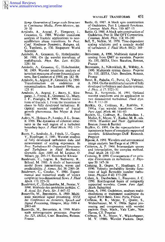
Syrup. Generation of Large-scale Structurein Continuous Media, Perm-Moscow, pp.29-30
Arn6odo, A., Argoul, F., Elezgaray, J.,Grasseau, G. 1988. Wavelet transformanalysis of fractals: applications to non-equilibrium phase transitions. In Proc.Conf. Nonlinear Dynamics, Bologna, ed.G. Turchetti, p. 130. Singapore: WorldScientific
Arn6odo, A., Grasseau, G., Holschneider,M. 1988. On the wavelet transform ofmultifractals. Phys. Rev. Lett. 61(20):2281-84
Arn6odo, A., Grasseau, G., Holschneider,M. 1989. Wavelet transform analysis ofinvariant measures of some dynamical sys-tems. See Combes et al 1989, pp. 182-96
Arn6odo, A., Argoul, F., Grasseau, G. 1990.Transformation en ondelettes etrenormalisation. See Lemari6 1990a, pp.125-91
Arn~odo, A., Argoul, F., Bacry, E., Elez-garay, J., Freysz, E., Grasseau, G., Muzy,J. F., Pouligny, B. 199l. Wavelet trans-form of fractals: I. From the transition tochaos to fully developed turbulence. I1.Optical wavelet transform of fractalgrowth phenomena. See Meyer & Paul1991
Aubry, N., Holmes, P., Lumley, J. L., Stone,E. 1988. The dynamics of coherent struc-tures in the wall region of a turbulentboundary layer. J. Fluid Mech. 192: 115-73
Bacry, E., Arn6odo, A., Frisch, U., Gagne,Y., Hopfinger, E. 1991. Wavelet analysisof fully developed turbulence data andmeasurement of scaling exponents. InProc. Turbulence 89: Organized Structuresand Turbulence in Fluid Mechanics,Grenoble, Sept. 1989, ed. M. Lesieur, O.M6tais, pp. 203-15. Dordrecht: Kluwer
Basdevant, C., Legras, B., Sadourny, R.,B~land, M. 1981. A study of barotropicmodel flows: intermittency, waves andpredictability. J. Atmos. Sci, 38:2305-26
Basdevant, C., Couder, Y. 1986. Experi-mental and numerical study of vortexcouples in two-dimensional flows. J. FluidMech. 173:225-51
Basdevant, C., Holschneider, M., Perrier, V.1990. M6thode des ondelettes mobiles. C.R. Acad. Sci. Paris, S~r. 1:647-52
Basseville, M., Benveniste, A. 1989. Multi-scale statistical signal processing. IEEElnt. Conference on Acoustics, Speech andSiynal Processin#, Glasyow, May 1989 4:2065~8
Basseville, M., Benveniste, A. 1990. Multi-scale autoregressive processes. PreprintNo. 525, IRISA, Univ. Beaulieu, Rennes,France
WAVELET TRANSFORMS 451
Battle, G. 1987. A block spin constructionof Ondelettes, Part I: Lemari6 functions.Commun. Math. Phys. 110:607-15
Battle, G. 1988. A block spin construction ofOndelettes, Part II: The QFT Connection.Commun. Math. Phys. 114:93-102
Bell, T., Nelkin, M. 1978. Time-dependentscaling relations and a cascade modelof turbulence. J. Fluid Mech. 88(2): 369-91
Benveniste, A. 1990. Multiscale signal pro-cessing: from QMF to wavelets. PreprintNo. 550, IRISA, Univ. Beaulieu, Rennes,France
Benveniste, A., Nikoukhah, R., Willsky, A.1990. Multiscale system theory. PreprintNo. 518, IRISA, Univ. Beaulieu, Rennes,France
Benzi, R., Paladin, G., Parisi, G., Vulpiani,A. 1984. On the multifractal nature of fullydeveloped turbulence and chaotic systems.J. Phys. A 17:3521-31
Benzi, R., Vergassola, M. 1991. Optimalwavelet transform and its application totwo dimensional turbulence. Fluid Dyn.Res. 8:117-26
Beylkin, G., Coifman, R., Rokhlin, V.1991a. Fast wavelet transform. Comm.Pure Appl. Math. 44:141-83
Beylkin, G., Coifman, R., Daubechies, I.,Mallat, S., Meyer, ¥., Ruskai, M. B., eds.1991b. Wavelets and Their Applications.Boston: Jones & Bartlett
Beylkin, G. 1991. On the representation ofoperators in bases of compactly supportedwavelets. Schlumberger-Doll Research.Preprint
Bijaoui, A. 1991. Wavelets and astronomicalimage analysis. See Farge et al 1991b
Calderon, A. P. 1964. Intermediate spacesand interpolation, the complex method.Stud. Math. 24:113-90
Castaing, B. 1989. Consequences d’un prin-cipe d’extremum en turbulence. J. Phys-ique 50:147-56
Castaing, B., Gagne, Y., Hopfinger, E. J.1990. Velocity probability density func-tions of high Reynolds number turbu-lence. Physica D 46:177-200
Cohen, A., Daubechies, I., Feauveau, J. C.1990. Biorthogonal bases of compactlysupported wavelets. Comm. Pure Appl.Math. Submitted
Cohen, A. 1990. Ondelettes, analyses multi-r6solutions et traitement num6rique dusignal. PhD thesis. Univ. Paris, France
Coifman, R. R., Meyer, Y., Quake, S.,Wickerhauser, M. V. 1990a. Signal pro-cessing and compression with waveletpackets. Dept. Math., Yale Univ., NewHaven, CT. Preprint
Coifman, R. R., Meyer, Y., Wickerhauser,M. V. 1990b. Wavelet Packets. Dept.
www.annualreviews.org/aronlineAnnual Reviews

452 FARGE
Math., Yale Univ., New Haven, CT. Preoprint
Combes, J. M., Grossmann, A., Tchamit-chian, P., eds. 1989. Wavelets, Time-Fre-quency Methods and Phase Space. 1stInt. Wavelet ConTr., Marseille, Dec. 1987,Inverse Probl. Theoret. Imaging. Springer
Dallard, T., Spedding, G. R. 1990. 2-Dwavelet transforms. Aerosp. Dept., Univ.South. Calif., Los Angeles, CA. Preprint
Daubechies, I., Grossmann, A., Meyer, Y.1986. Painless nonorthogonal expansions.J. Math. Phys. 27:1271-83
Daubechies, I., Paul, T. 1987. Wavelets andapplications. In Proceedings of the 8thInternational Congress of MathematicalPhysics, ed. M. Mebkbout, R. Seneor. Sin-gapore: World Scientific
Daubechies, I., Paul, T. 1988. Time fre-quency localization operators--a geo-metric phase-space approach: II The useof dilations. Inverse Probl. 4:661-81
Daubechies, I. 1988. Orthonormal bases ofcompactly supported wavelets. Comm.Pure Appl. Math. 41(7): 909-96
Daubechies, I. 1989. Orthonormal bases ofwavelets with finite support--Connectionwith discrete filters. See Combes et a11989,pp. 38~i6
Daubechies, I. 1990. The wavelet transform,time-frequency localization and signalanalysis. IEEE Trans. Inf Theory 36:961
Daubechies, I. 1991. Ten lectures onwavelets. CBMS Lecture Notes Series.SIAM
Daubechies, I., Mallat, S., Willsky, A. 1991.Wavelet transforms and multiresolutionsignal analysis. IEEE Trans. Inf Theory.In press
Delprat, N., Escudi+, B., Guillemain, P.,Kronland-Martinet, R., Tehamitchian,P., Torr6sani, B. 1991. Asymptotic wave-let and Gabor analysis; extraction ofinstantaneous frequencies. See Daubech-ies et al 1991
Desnjanski, V. N., Novikov, E. A. 1974.Model of cascade processes in turbulentflows. Appl. Math. Mech. 38(3): 507 (In Russian)
Dutilleux, P. 1989. An implementation of thealgorithme fi trous to compute the wavelettransform. See Combes et al 1989, pp.298-304
Duval-Destin, M., Menu, J. P. 1989. Wavelettransform: a new basic spatial operator forvisual psychoplaysics. Vision Res. Sub-mitted
Duval-Destin, M., Murenzi, R. 1991. Spatio-temporal wavelet transform. Preprint TR/VI/91/49, CERFACS, Toulouse, France
Duval-Destin, M., Muschietti, M. A., Tor-r6sani, B. 1991. From continuous waveletsto wavelet packets. Preprint CPT, Cent.
Phys. Th6orique, CNRS-Luminy, Mar-seille, France
Escudi+, B., Torr6sani, B. 1989. Waveletanalysis of asymptotic signals. PreprintCPT-89/P.2304, Cent. Phys. Th6orique,CNRS-Luminy, Marseille, France
Esteban, D., Galand, C. 1977. Applicationof Quadrature Mirror Filters to split bandvoice coding schemes. Proc. 1977 IEEEInt. Conf. Acoustic, speech and signal pro-cessing, Hartford, pp. 191-95
Everson, R. M., Sirovich, L. 1989. A Surveyof wavelet analysis applied to turbulencedata. Report 89-182, Cent. Fluid Mech.Turbulence Comput., Brown Univ.,Providence, RI
Everson, R., Sirovich, L., Sreenivasan, K. R.1990. Wavelet analysis of the turbulent jet.Phys. Lett. A 145:314
Falconer, K. J. 1991. Wavelets, fractals andorder-two densities. See Farge et al 1991b
Farge, M., Rabreau, G. 1988a. Wavelettransform to analyze coherent structuresin two-dimensional turbulent flows. Proc.Scaling, Fractals and Nonlinear Variabilityin Geophysics 1, Paris, June 1988
Farge, M., Rabreau, G. 1988b. Transform6een ondelettes pour d6tecter et analyser lesstructures coh6rentes dans les 6coulementsturbulents bidimensionnels. C. R. Acad.Sci. Paris Ser. H 307:1479-86
Farge, M., Sadourny, R. 1989. Wave-vortexdynamics in rotating shallow water. J.Fluid Mech. 206:433~52
Farge, M., Holschneider, M. 1989. Two-dimensional wavelet analysis of two-dimensional turbulent flows. Proc. Sca-ling, Fractals and Nonlinear Variability inGeophysics II, Barcelone, March 1989
Farge, M., Holschneider, M., Colonna, J. F.1990a. Wavelet analysis of coherent struc-tures in two-dimensional turbulent flows.In Topological Fluid Mechanics, ed. H. K.Moffatt, pp. 765-76. Cambridge: Cam-bridge Univ. Press
Farge, M. 1990. Transform6e en ondelettescontinue et application gtla turbulence.Journ. Annu. Soc. Math. France, May1990:17-452
Farge, M., Holschneider, M. 1991. Interpre-tation of two-dimensional turbulenceenergy spectrum in terms of quasi-singu-larity in some vortex cores. Europhys. Lett.15(7): 737-43
Farge, M., Guezennec, Y., Ho, C. M., Mene-veau, C. 1990b. Continuous waveletanalysis of coherent structures. Proc. Sum-mer Prog. Cent. Turbulence Res., StanfordUniv. NASA-Ames, Stanford, CA
Farge, M. 1991a. Continuous wavelet trans-form application to turbulence. See Beyl-kin et al 1991b
Farge, M. 1991b. L’6volution des th6ories de
www.annualreviews.org/aronlineAnnual Reviews

la turbulence. To appear in Chaos etD~terminisme, Collection Points-Sciences,Le Seuil
Farge, M., Holschneider, M., Philipovitch,T. 1991a. Formation et stabilit6 des quasi-singularit6s r -t/~ en turbulence bidi-mensionnelle. C. R. Acad. Sc. Paris. Sub-mitted
Farge, M., Hunt, J, Vassilicos, C., eds.1991b. Wavelets, Fractals and FourierTransform: New Developments and NewApplications. Oxford: Oxford Univ. Press.In press
Farge, M., Goirand, E., Wickerhauser, V.1991c. Wavelet packets analysis, com-pression and filtering of two-dimensionalturbulent flows. LMD, Ecole Normal~Sup6rieure, Paris. Preprint
Feauveau, J. C. 1989. Filtres miroirs con-jugu6s: une th6orie pour les filtres miroirsen quadrature et l’analyse multir6solutionpar ondelettes. C. R. Acad. Sci. Paris, Sbr.H 308:1479-86
Feauveau, J. C. 1990. Analyse multi-r+solution par ondelettes. C. R. Acad.Sci. Paris, S~r. 1309:853-56
Flandrin, P. 1988. Time-frequency and time-scale. IEEE Fourth Annu. ASSP WorkshopSpectrum Estimation and Modeling,Minneapolis, August 1988, pp. 77-80
Flandrin, P. 1990. Wavelets and relatedtime-scale transforms. SPIE Proc. Ad-vanced Signal Processing Algorithms, Ar-chitectures and Implementations, ed. F.T. Luk, 1348:2-13
Flandrin, P., Rioul, O. 1990. Affine smooth-ing of the Wigner-Ville distribution. 1EEEICASSP Conference, Albuquerque, April1990, pp. 2455-58
Flandrin, P. 1991a. Wavelet analysis andsynthesis of fractional Brownian motion.In Wavelet Transforms and Multi-resolution Signal Analysis, ed. I. Daubech-ies, S. Mallat, A. Willsky, IEEE Trans.Inf Theory, special issue
Flandrin, P. 1991b. Fractional Brownianmotion and wavelets. See Farge et al 1991 b
Freysz, E., Pouligny, B., Argoul, F., Arn6-odo, A. 1990. Optical wavelet transformof fractal aggregates. Phys. Rev. Lett. 64:745
Frick, P. G. 1983. Hierarchical model oftwo-dimensional turbulence. Magneto-hydrodynamics 19(1): 48-53 (From Rus-sian)
Frick, P. G. 1984. Two-dimensional MHD-turbulence: Hierarchical model. Magneto-hydrodynamics" 20(3) (From Russian)
Frick, P. G. 1986a. A cascade model of two-dimensional turbulent convection. FluidMech. Soy. Res. 15(2): 80-92 (From Rus-sian)
Frick, P. G. 1986b. Modeling of cascade pro-
WAVELET TRANSFORMS 453
cess in two-dimensional turbulent con-vection. J. Appl. Mech. Tech. Phys. 27(2):221-28 (From Russian)
Frick, P. G. 1987. Modeling of the space-time structure of developed two-dimen-sional turbulent convection. Fluid Mech.Soy. Res. 16(3): 49-54 (From Russian)
Frick, P. G., Mikishcv, A. V. 1990. Inves-tigation of local and integral charac-teristics of developed two-dimensionalturbulence using the hierarchical model.Second Worm Congr. Comput. Mech.,August 1990, Stutt#art
Frick, P. G., Zimin, V. D. 1991. Hierarchicalmodels of turbulence. See Farge et al1991b
Frisch, U., Sulem, P. L. 1975. Remarquesur la multiplication dans les espaces deSobolev et application aux 6quationsd’Euler d’un fluide illimit6. C. R. Acad.Sci. Paris, Sbr. A 280:1117-20
Frisch, U., Sulem, P. L., Nelkin, M. 1978. Asimple dynamical model of intermittentfully developed turbulence. J. Fluid Mech.87:719-36
Frisch, U., Vergassola, M. 1990. A pre-diction of the multifractal model: theintermediate dissipation range. Europhys.Lett. Submitted
Gabor, D. 1946. Theory of communication.J. Inst. Electr. Eng, 93(1II): 429-57
Gasquet, C., Witomski, P. 1990. Analyse deFourier et Applications: Filtragre, Cal-cul Numerique, Ondelettes. Paris: Masson
Ghez, J. M., Vaienti, S. 1989. On the waveletanalysis for multifractal sets. J. Stat. Phys.57(12): 415-20
Gledzer, E. B., Dolzhansky, F. B., Obukhov,A. M. 1981. Systems of hydrodynamicaltype and their applications. C. R. Acad.Sci., Moscow (In Russian)
Glowinski, R., Lawton, W. M., Ravachol,M., Tencnbaum, E. 1990. Wavelet solu-tion of linear and nonlinear elliptic, para-bolic and hyperbolic problems in onespace dimension. 9th Int. Conf Appl. Sci.Eng., SLAM, Philadelphia
Goupillaud, P., Grossmann, A., Morlet, J.1984. Cycle-octave and related transformsin seismic signal analysis. Geoexploration23:85-105
Grossmann, A. 1988. Wavelet transformsand edge detection. Stochastic" Processes"in Physics and En#ineering, ed. P. Blan-chard, L. Streit, M. Hazewinkel. Boston:Reidel
Grossmann, A., Morlet, J. 1984. Decompo-sition of Hardy functions into square inte-grable wavelets of constant shape. SIAMJ. Math. Anal. 15(4): 723-36
Grossmann, A., Paul, T. 1984. Wave func-tions on subgroups of the group of affinecanonical transformations. Resonances,
www.annualreviews.org/aronlineAnnual Reviews
454 FARGE
Models and Phenomena, Lecture Notes inPhysics, No. 211. Berlin: Springer-Verlag
Grossmann, A., Morlet, J. 1985. Decompo-sition of functions into wavelets of con-stant shape, and related transforms. InMathematics÷Physics, Lectures on Re-cent Results, ed. L. Streit, 1: 135-65.Singapore: World Scientific
Grossmann, A., Morlet, J., Paul, T. 1985.Transforms associated to square inte-grable group representations I: generalresults. J. Math. Phys. 26:2473-79
Grossmann, A., Morlet, J., Paul, T. 1986.Transforms associated to square inte-grable group representations II: examples.Ann. Inst. Henri Poincark, Phys. Thkorique45:293-309
Grossmann, A., Holschneider, M., Kron-land-Martinet, R., Morlet, J. 1987. Detec-tion of abrupt changes in sound signalswith the help of wavelet transforms. InAdvances in Electronics and Electron Phys-ics, Suppl. 19, Inverse Problems, pp. 289-306. Academic
Grossmann, A., Kronland-Martinent, R.1988. Time-and-scale representationsobtained through continuous wavelettransforms. In Signal Processing IV." The-ories and Applications, EURASIP 88, ed.J. L. Lacoume, A. Chehikian, N. Martin,J. Malbos, pp. 675-82. Amsterdam: Else-vier
Grossmann, A., Kronland-Martinet, R.,Mor/et, J. 1989. Reading and under-standing continuous wavelet transforms.See Combes et al 1989, pp. 2 20
Guillemain, P. 1991. Application of waveletanalysis in NMR spectroscopy. See Meyer& Paul 1991
Haar, A. 1909. Zur Tlaeorie der Ortho-gonalen Funktionensysteme. Gotttngen,Juli 1909
Holschneider, M. 1988a. L’analyse d’objetsfractals et leur transform6e en ondelettes.PhD thesis. Univ. d’Aix-Marseille II,Luminy, France
Holschneider, M. 1988b. On the wavelettransformation of fractal object. J. Stat.Phys. 50:953-93
Holschneider, M., Kronland-Martinct, R.,Morlet, J., Tchamitchian, P. 1988. The"algorithme it trous." IEEE Trans. ASSP.Submitted
Holschneider, M., Kronland-Martinet, R.,Morlet, J., Tchamitchian, P. 1989. A real-time algorithm for signal analysis with thehelp of the wavelet translbrm. See Combeset al 1989, pp. 286-97
Holschneider, M., Tchamitchian, P. 1989.Pointwise analysis of Riemann’s non-differentiable function. Inventiones Math.Submitted
Holschneider, M. 1990. Inverse Radon
transform through inverse wavelet trans-form. lnverse Probl. Submitted
Holschneider, M., Tchamitchian, P. 1990.R6gularit6 locale de la fonction "non-diff6rentiable" de Riemann. See Lemari61990a, pp. 102-24
Holschneider, M. 1991. Wavelet Analysis.Textbook submitted to Springer
Jaffard, S. 1989a. Exposants de H61der endes points donn6s et coefficients d’on-delettes. C. R. Acad. Sci. Paris, SOt. 1308:79-81
Jaffard, S. 1989b. Construction of waveletson open sets. See Combes et al 1989, pp.247-52
Jaffard, S., Meyer, Y. 1989. Bases d’on-delettes dans des ouverts de R". J. Math.Pures Appl. 68:95-108
Jaffard, S. 1990a. Construction et propri6t6sdes bases d’ondelettes. Remarques sur lacontrtSlabilit6 exacte. PhD thesis, l’EcolePolytechnique, Palaiseau, France
Jaffard, S. 1990b. Wavelet methods for fastresolution of elliptic problems. Preprint90/5, Lab. Math. Mod61isation, Ecole Nat.Ponts-et-Chaussees, La Courtine, Noisy-le-Grand, France
Jaffard, S. 1991a. Detection and identi-fication of singularities by the continuouswavelet transform. Preprint, Lab. Math.Mod61isation, Ecole Nat. Ponts-et-Chaus-sees, La Courtine, Noisy-le-Grand, France
Jaffard, S. 1991b. Orthonormal and con-tinuous wavelet transform: algorithmsand applications to the study of pointwiseproperties of functions. See Farge et al1991b
Kim, J., Moin, P., Moser, R. 1987. Tur-bulence statistics in fully developed chan-nel flow at low Reynolds number. J. FluidMech. 177:133-66
Kline, S. J., Reynolds, W. ~., Schraub, F.A., Runstadler, P. W. 1967. The structureof turbulent boundary layers. J. FluidMech. 30(4): 741-73
Kolmogorov, A. M. 1961. A refinement ofprevious hypotheses concerning the localstructure of turbulence in viscous incom-pressible fluid at high Reynolds number.J. Fluid Mech. 177:133-66
Kraichnan, R. H. 1974. On Kolmogorov’sinertial-range theories. J. Fluid Mech. 62:305-30
Kronland-Martinet, R., Morlet, J.,Grossmann, A. 1987. Analysis of soundpatterns through wavelet transforms. Int.J. Pattern Anal. Artif. Intell. 1(2): 273-302
Kronland-Martinet, R. 1988. The use of thewavelet transform for the analysis, syn-thesis and processing of speech and musicsounds. Comput. Music J. MIT Press, 12:4
www.annualreviews.org/aronlineAnnual Reviews

Latto, A., Tenenbaum, E. 1990. Compactlysupported wavelets and the numericalsolution of Biirgers equation. C. R. Acad.Sci. Paris, S~r. 1311: 903-9
Laufer, J. 1975. New trends in experimentalturbulence research. Annu. Rev. FluidMech. 7:307-26
Lemarib, P. G., Meyer, Y. 1986. Ondeletteset bases hilbertiennes. Rev. Mat. IberoAm.2:1-18
LemariS, P. G. 1988. Ondelettes h loeal-isation exponentielle. J. Math. Pures Appl.67:227-36
Lemari+, P. G., ed. 1990a. Les Ondelettesen 1989. Lecture Notes in Mathematics,Berlin: Springer
LemariS, P. G. 1990b. Introduction ~i la thro-tie des ondelcttes. See Lemari6 1990a, pp.1-13
LemariS, P. G. 1990c. Analyse multi-rchelleset ondelettes ~i support compact. SeeLemari6 1990a, pp. 26-38
Leonard, A. 1985. Computing three-dimen-sional incompressible flows with vortexelements. Annu. Rev. Fluid Mech. 17: 523-59
Liandrat, J., Perrier, V., Tchamitchian, P.1989. Numerical resolution of the regu-larized B/irgers equation using the wavelettransform. See Meyer & Paul 1991
Liandrat, J., Tehamitehian, P. 1990. Res-olution of the 1D regularized Biirgersequation using a spatial wavelet approxi-mation-Algorithm and numerical re-sults. ICASE Report, NASA Langley,Hampton, Virginia
Liandrat, J., Moret-Baifly, F. 1990. Thewavelet transform: some applications tofluid dynamics and turbulence. Eur. J.Mech. B/Fluids 9(1): 1-19
Liandrat, J., Perrier, V., Tchamitchian, P.1991. Numerical resolution of nonlinearpartial differential equations using thewavelet transform. See Beylkin et al1991b
Lumley, J. L. 1981. Coherent structures inturbulence. In Transition and Turbulence,ed. R. E. Meyer, pp. 215-41. New York:Academic
Maday, Y., Perrier, V., Ravel, J. C. 1990.Adaptativit~ dynamique sur bases d’on-delettes pour l’approximation d’rquationsaux drriv~es partielles. C. R. Acad. Sci.Paris. Submitted
Mallat, S. 1988. Review of multifrequencychannel decompositions of images andwavelet models. In Acoustic, Speech andSignal Processing, Multidimensional Sig-nal Processing, IEEE (special issue)
Mallat, S. 1989a. A theory for multi-resolution signal decomposition: thewavelet representation. IEEE, Trans. onPattern Anal. Machine Intell. 2:7
WAVELET TRANSFORMS 455
Mallat, S. 1989b. Multiresolution approxi-mations and wavelet orthonormal basesof L2(R). Trans. Am. Math. Soc. 315: 69-87
Mallat, S. 1989c. Multiresolution approxi-mation and wavelets. Report GRASPLab., Dept. Comput. Inf. Sci., Univ.Pennsylvania, Philadelphia, PA
Mallat, S. 1989d. Multiresolution approachto wavelets in computer vision. See Com-bes et al 1989. (2nd ed. 1990, p. 313)
Mallat, S., Hwang, L. H. 1990. Singularitydetection and processing with wavelets.Courant lnst. Tech. Rep. No. 549, NewYork, NY
Mallat, S., Zhong, S. 1990. Complete signalrepresentation with multiscale edges.Courant lnst. Tech. Rep. No. 483, NewYork, NY
Mallat, S., Zhong, S. 1991. Wavelet trans-form maxima and multiscale edges. SeeBeylkin et al 1991b
Mandelbrot, B. 1974. Intermittent tur-bulence in self-similar cascades: diver-gence of high moments and dimension ofcarrier. J. Fluid Mech. 62:331-58
McWilliams, J. 1984. The emergence of iso-lated coherent vortices in turbulent flow.J. Fluid Mech. 146:21-433
Meneveau, C. 1991 a. Analysis of turbulencein the orthonormal wavelet represen-tation. J. Fluid Mech. In press
Meneveau, C. 1991b. Wavelet analysis ofturbulence: the mixed energy cascade. SeeFarge et al 1991b
Meneveau, C. 1991. Dual spectra and mixedenergy cascade of turbulence in the wave-let representation. Phys. Rev. Lett. 66:1450
Meyer, Y. 1985. Principe &incertitude, baseshilbertiennes et algrbres d’oprrateurs.Sdminaire Bourbaki, 1985-86, 662, AstOr-isque, Socidt~ Mathdmatique de France,Paris, France
Meyer, Y. 1986. Ondelettes et fonctionssplines. Sdminaire Equations aux ddrivdespartielles, Cent. Math. Ecole Polytech.,Palaiseau, France
Meyer, Y. 1987a. Ondelettes, fonetionssplines et analyse gradure. Rapport CER-EMADE, No. 8703, Univ. Paris-Dauphine, Paris, France
Meyer, Y. 1987b. Wavelets and operators.Rapport CEREMADE, No. 8704, Univ.Paris-Dauphine, Paris, France
Meyer, Y. 1988. Orthonormal wavelets.Congr. lnt. Phys. Math., Swansea, July
Meyer, Y. 1989a. Ondelettes, filtres miroirsen quadrature traitement numrrique del’image. Gaz, Math. 40:31-42
Meyer, Y. 1989b. Orthonormal wavelets. SeeCombes et al 1989, pp. 21-37
Meyer, Y. 1989c. Ondelettes, filtres miroirs
www.annualreviews.org/aronlineAnnual Reviews
456 FARGE
en quadrature et traitement num6rique del’image. See Lemari6 1990a, pp. 14-25
Meyer, Y. 1990a. Ondelettes et op6rateurs,tome I. ActualitOs Math~matiques. Paris:Hermann
Meyer, Y. 1990b. Le calcul scientifique, lesondelettes et les filtres miroirs en quad-rature. Rapport CEREMADE, No. 9007,Univ. Paris-Dauphine, Paris, France
Meyer, Y. 1990c. Ondelettes et applications.J. Annu. Soc. Math. France, May 1990,Soc. Fran~aise Math., Paris, France, pp.1-15
Meyer, Y., Paul, T., eds. 1991. Wavelets andApplications. Proceedings of the SecondInternational Wavelet Conference, Mar-seille, June 1989. Paris: Masson. In press
Mikishev, A. V., Frick, P. G. 1989. Inter-mittence in ideal two-dimensional mag-netohydrodynamic turbulence. Magneto-hydrodynamics 25(1): 127-30 (From Rus-sian)
Mikishev, A. V., Frick, P, G. 1990. On thespectral laws in two-dimensional tur-bulent flow with linear friction. Magneto-hydrodynamics 26(1): 136-39 (From Rus-sian)
Moret-Bailly, F., Chauve, M. P., Liandrat,J., Tchamitchian, P. 199 I. Determinationsdu nombre de Reynolds de transition dansune ~tude de touche limite sur un disquetournant. C. R. Acad. Sci. Paris, Sub-mitted
Morlet, J. 1981. Sampling theory and wavepropagation. Proc. 51st Annu. Meet. Soc.Explor. Geophys., Los Angeles
Morlet, J. 1983. Sampling theory and wavepropagation. NATO ASI, Vol. F1, Issueson Acoustic Signal~Image Processing andRecognition, ed. C. H. Chert. Berlin:Springer
Murenzi, R. 1989. Wavelet transformsassociated to the N-dimensional Eucli-dean group with dilatations: signal inmore than one dimension. See Combes etal 1989, pp. 239-46
Murenzi, R. 1990. Ondelettes multi-dimensionnelles et application ~ l’analysed’images. PhD thesis. Univ. Cathol. Lou-vain, Louvain-la-Neuve, Belgium
Muzy, J. F., Bacry, E., Arn+odo, A, 1991.Wavelets and multifractal formalism forsingular signals. Phys. Rev. Lett. Sub-mitted
Nakano, T. 1988. Direct interactionapproximation of turbulence in the wavepacket representation. Phys. Fluids 31:1420
Nguyen Duc, J., Sommeria, J. 1988. Experi-mental characterization of steady two-dimensional vortex couples. J. FluMMech.192:175-92
Otaguro, T., Takagi, S., Sato, H. 1989. Pat-
tern search in a turbulent signal usingwavelet analysis. Proc. 21st Japan Syrup.on Turbulence. Tokyo, Japan
Parisi, G., Frisch, U. 1985, Fully developedturbulence and intermittency. In Proc.International School on Turbulence andPredictability in Geophysical Fluid Dynam-ics and Climate Dynamics, ed. M. Ghil, R.Benzi, G. Parisi, pp. 71-88, Amsterdam:North-Holland
Paul, T. 1984. Functions analytic on the half-plane as quantum mechanical states. J.Math. Phys. 25:11
Paul, T. 1985a. Aflinc coherent states andthe radial Schr6dinger equation. Ann. Inst.Henri Poincar& Submitted
Paul, T. 1985b. Ondelettes et m6caniquequantique. PhD thesis. Univ. Aix-Mar-seille II, Luminy, Marseille, France
Paul, T. 1986. A characterization dilationanalytic operators. In Schr6dinger oper-ators, Aarhus, 1985, Lecture Notes inMathematics, 1218. Berlin: Springer
Paul, T. 1989. Wavelets and path integrals.SeeCombes et al 1989, pp. 204-8
Perrier, V. 1989. Toward a method for solv-ing Partial Differential Equations usingwavelet bases. See Combes et al 1989, pp.269-82
Perrier, V., Basdevant, C. 1989. Lad~composition en ondelettes p6riodiques,un outil pour l’analyse de champs inhomo-g6nes. Th6orie et algorithmes. La Rech-erche Abrosp. 3:53~57
Pettier, V. 1991a. Ondelettes et simulationnum6rique. PhD thesis. Univ. Paris VI,Paris, France
Perrier, V. 1991b. Apport des ondelettes ~.la r~solution num+rique d’6quations auxd~riv~es partielles. J. Soc. Math. Appl. Ind.In press
Qian, J. 1988. Cascade model of turbulence.Phys. Fluids 31(10): 1865-74
Rioul, O. 1987. Ondelettes et traitementdu signal. Rapport d’option de Mathb-matiques, Ecole Polytcch., Palaiseau,France
Rioul, O. 1991. A unifying multiresolutiontheory for the discrete wavelet transform,regular filter banks and pyramid trans-forms. IEEE Trans. Acoustics, Speech andSignal Processing. Submitted
Saracco, G., Tchamitchian, P. 1988. A studyof acoustic transmission of transient sig-nal in an inhomogeneous medium with thehelp of the wavelet transform--Appli-cation to an air-water plane interface. InElectromagnetic and Acoustic Scattering:Detection and lnverse Problem, ed. C. Bur-rely, P. Chiapetta, B. Torr6sani. Mar-seille: World Scientific
Saracco, G., Grossmann, A., Tchamitchian,P. 1989. Use of wavelet transforms in the
www.annualreviews.org/aronlineAnnual Reviews

study of propagator of transient acousticsignals across a plane interface betweentwo homogeneous media. See Combes etal 1989, pp. 139-46
Stromberg, J. O. 1981. A modified Haar sys-tem and higher order spline systems. Conf.Harmonic Analysis in Honor of AntoniZygmund, II, ed. W. Becker et al, pp. 475-93. Wadworth math. series
Tchamitchian, P. 1986. Calcul symboliquesur les op6rateurs de Calderon-Zygmundet bases inconditionnelles de L2(R). C. Acad. Sci. Paris, S~r. 1303:6
Tchamitchian, P. 1987. Biorthogonalit6 etth6orie des op6rateurs. Rev. Math.Iberoam. 3:2
Tchamitchian, P. 1989a. Bases d’ondeletteset int6grales singuli6res: analyse desfonctions et calcul sur les op6rateurs.Thdse d’habilitation ~ diriger desrecherches. Univ. Aix-Marseille II,Luminy, Marseille, France
Tchamitchian, P. 1989b. About wavelets andelliptic operators. See Combes et al 1989,pp. 263~58
Tchamitchian, P. 1989c. Ondelettes etint6grale de Cauchy sur les courbeslipehitziennes. Ann. Math. 129:641
Tchamitchian, P., Torr6sani, B. 1991. Ridgeand skeleton extraction from the wavelettransform. See Beylkin 1991b
Tennekes, H., Lumley, J. L. 1972. A FirstCourse in Turbulence. Cambridge: MITPress
Torr6sani, B. 1991. Time-frequency repre-sentations: wavelet packets and optimaldecomposition. Ann. Inst. H. Poincar~,Phys. Th~orique. In press
Townsend, A. A. 1956. The Structure of Tur-bulent Shear Flow. Chapter 6. Cambridge:Cambridge Univ. Press
WAVELET TRANSFORMS 457
Vergassola, M., Frisch, U. 1990. Scalingexponents for global and local self-similarprocesses. Physica D. Submitted
Vetterli, M., Herley, C. 1990a. Wavelets andfilter banks: theory and design. IEEETrans. Acoustics, Speech Signal Process-ing. Submitted
Vetterli, M., Herley, C. 1990b. Wavelets andfilter banks: relationship and new results.IEEE Trans. ,4 coustics, Speech Signal Pro-cessing. In press
Vetterli, M., Herley, C. 1990c. Linear phasewavelets. IEEE Trans. Acoustics, SpeechSignal Processing. In press
Wickerhauser, M. V. 1991. INRIA lectureson wavelet packet algorithms. Preprint,Dept. Math., Yale Univ., New Haven, CT
Yamada, M., Ohkitani, K. 1990a. Orthonor-mal wavelet expansions and its applicationto turbulence. Prog. Theor. Phys. 83:819
Yamada, M., Ohkitani, K. 1990b. Orthonor-mal wavelet analysis of turbulence.Preprint, Res. Inst. Math. Sci., KyotoUniv., Kyoto, Japan
Zimin, V. D. 1981. Hierarchical model ofturbulence. Izv. Atmos. Ocean Phys. 17:941-49 (From Russian)
Zimin, V. D., Frick, P. G., Shaidurova, T.E. 1986. Hierarchical bases for turbulentfields describing. Preprint, Inst. Con-tinuous Media Mech. Korolyov 1, Perm,Soviet Union (In Russian)
Zimin, V. D., Frick, P. G. 1988. TurbulentConvection. Moscow: Nauka (In Russian)
Zimin, V. D. 1990a. Hierarchy model of tur-bulence. 6th Beer-Sheva Int. Sem. MHDFlows Turbulence, Jerusalem
Zimin, V. D. 1990b. Hierarchy model of tur-bulence. Int. Syrup. Generation of large-scale structure in continuous media, Perm-Moscow, June, p. 263
References added in proof
Farge, M. 1991c. Wavelets and turbulence.INSU Summer School on Geophys. FluidDyn., July 1991, Roscoff
Granlund, G. H. 1978. In search of a generalpicture processing operator. Comput.Graphics Image Process. 8:155-73
www.annualreviews.org/aronlineAnnual Reviews