Wavefront reconstruction for adaptive optics reconstruction for adaptive optics ... System matrix...
54
Wavefront reconstruction for adaptive optics Marcos van Dam and Richard Clare W.M. Keck Observatory
Transcript of Wavefront reconstruction for adaptive optics reconstruction for adaptive optics ... System matrix...
Wavefront reconstruction for adaptive
optics
Marcos van Dam and Richard Clare
W.M. Keck Observatory
We borrowed slides from the following people:Lisa Poyneer
Luc Gilles
Curt Vogel
Corinne Boyer
Mahalo!
Friendly people
Imke de Pater et al
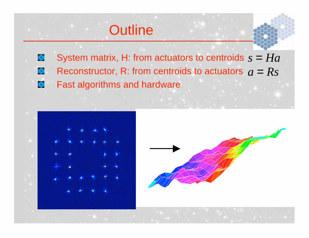
System matrix, H: from actuators to centroids
Reconstructor, R: from centroids to actuators
Fast algorithms and hardware
Outline
Has =
Rsa =
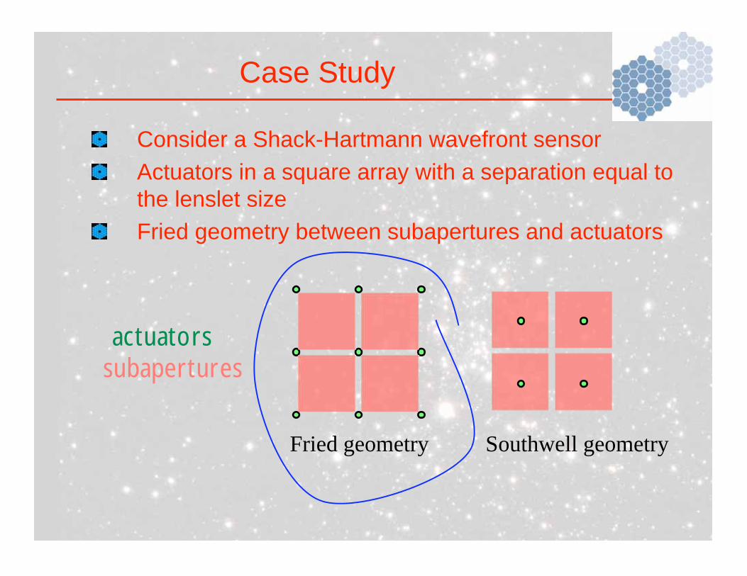
Consider a Shack-Hartmann wavefront sensor
Actuators in a square array with a separation equal to
the lenslet size
Fried geometry between subapertures and actuators
Case Study
Fried geometry Southwell geometry
actuators subapertures
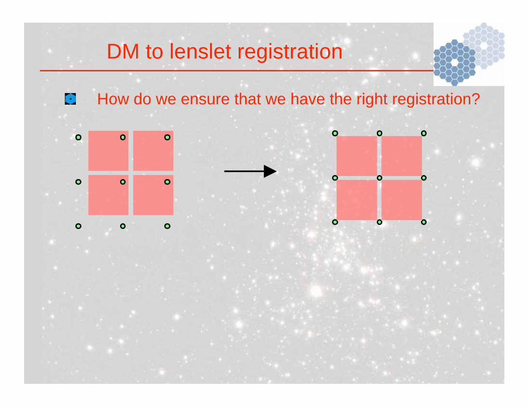
How do we ensure that we have the right registration?
DM to lenslet registration
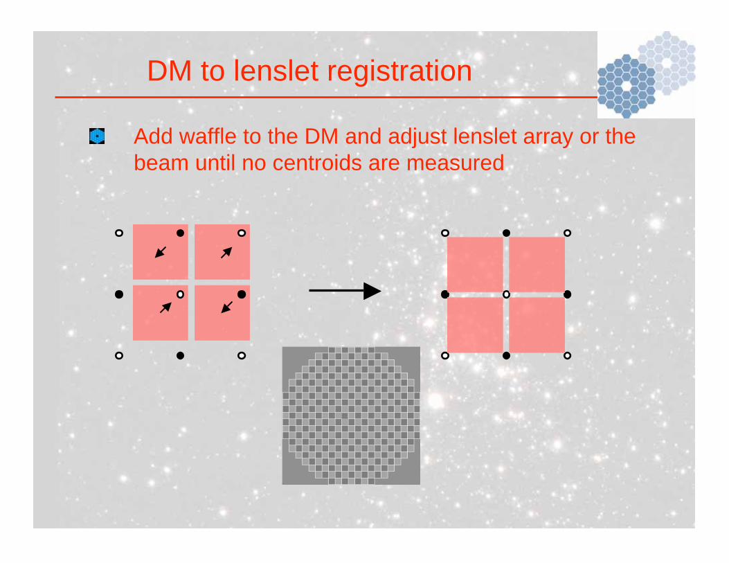
Add waffle to the DM and adjust lenslet array or the
beam until no centroids are measured
DM to lenslet registration
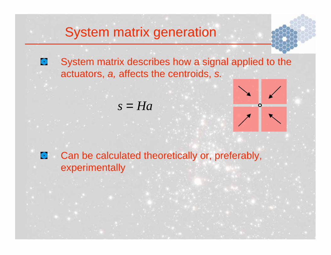
System matrix describes how a signal applied to the
actuators, a, affects the centroids, s.
Can be calculated theoretically or, preferably,
experimentally
System matrix generation
Has =
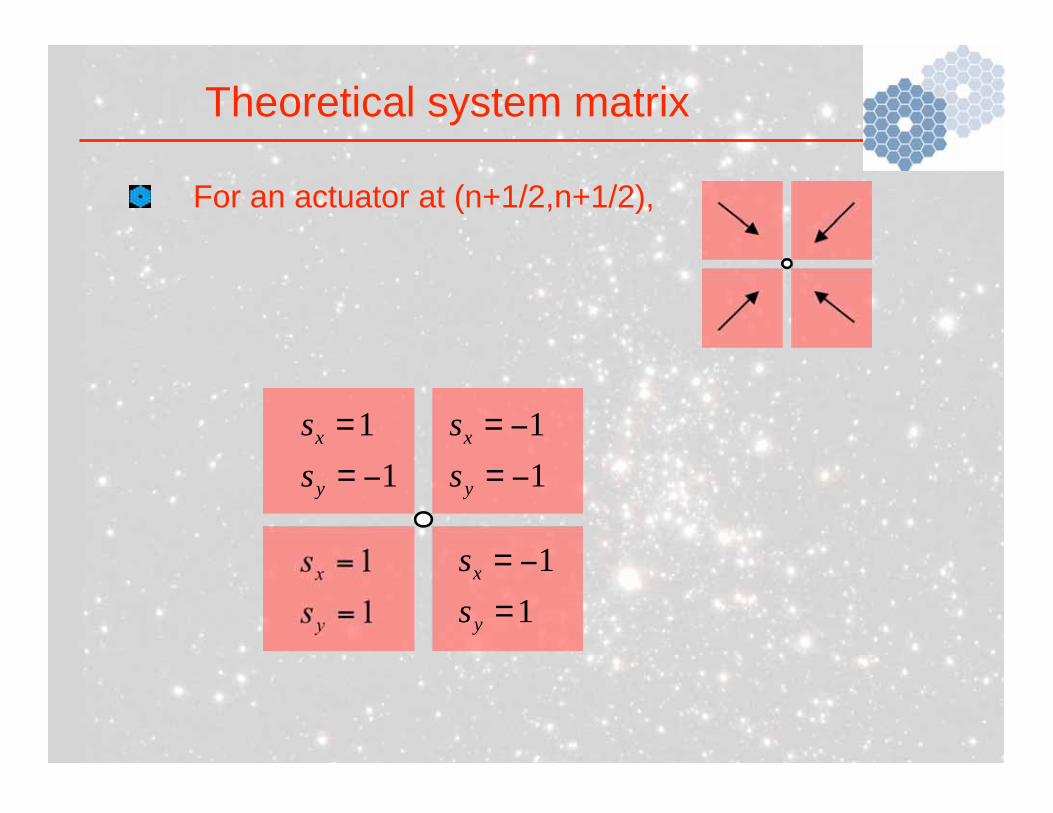
For an actuator at (n+1/2,n+1/2),
Theoretical system matrix
1
1
=
=
y
x
s
s
1
1
=
=
y
x
s
s
1
1
=
=
y
x
s
s
1
1
=
=
y
x
s
s
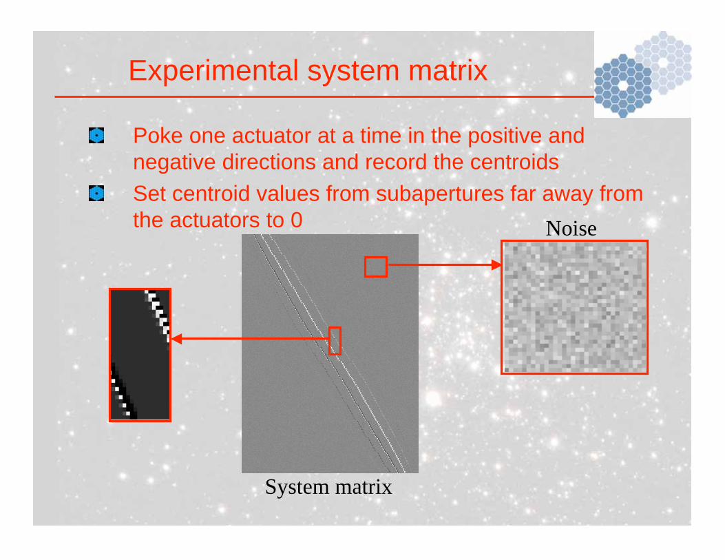
Poke one actuator at a time in the positive and
negative directions and record the centroids
Set centroid values from subapertures far away from
the actuators to 0
Experimental system matrix
System matrix
Noise
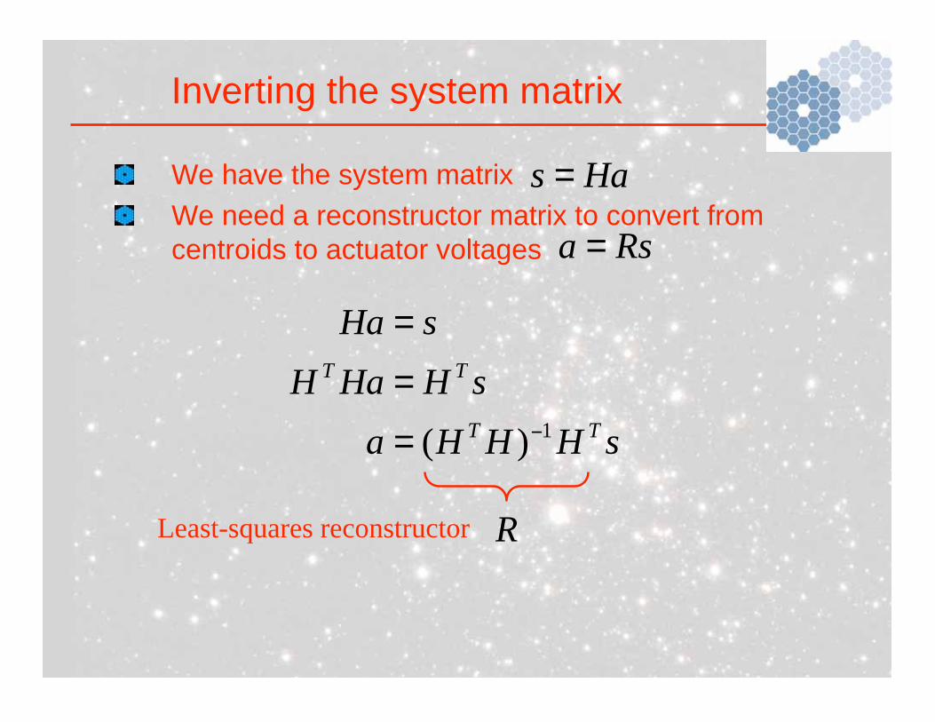
We have the system matrix
We need a reconstructor matrix to convert from
centroids to actuator voltages
Inverting the system matrix
Has =
Rsa =
sHHHa
sHHaH
sHa
TT
TT
1)(=
=
=
RLeast-squares reconstructor
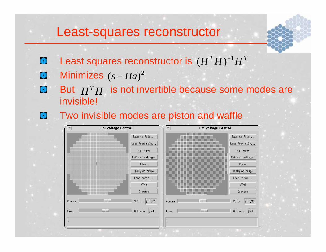
Least squares reconstructor is
Minimizes
But is not invertible because some modes are
invisible!
Two invisible modes are piston and waffle
Least-squares reconstructor
HHT
TTHHH
1)(2)( Has
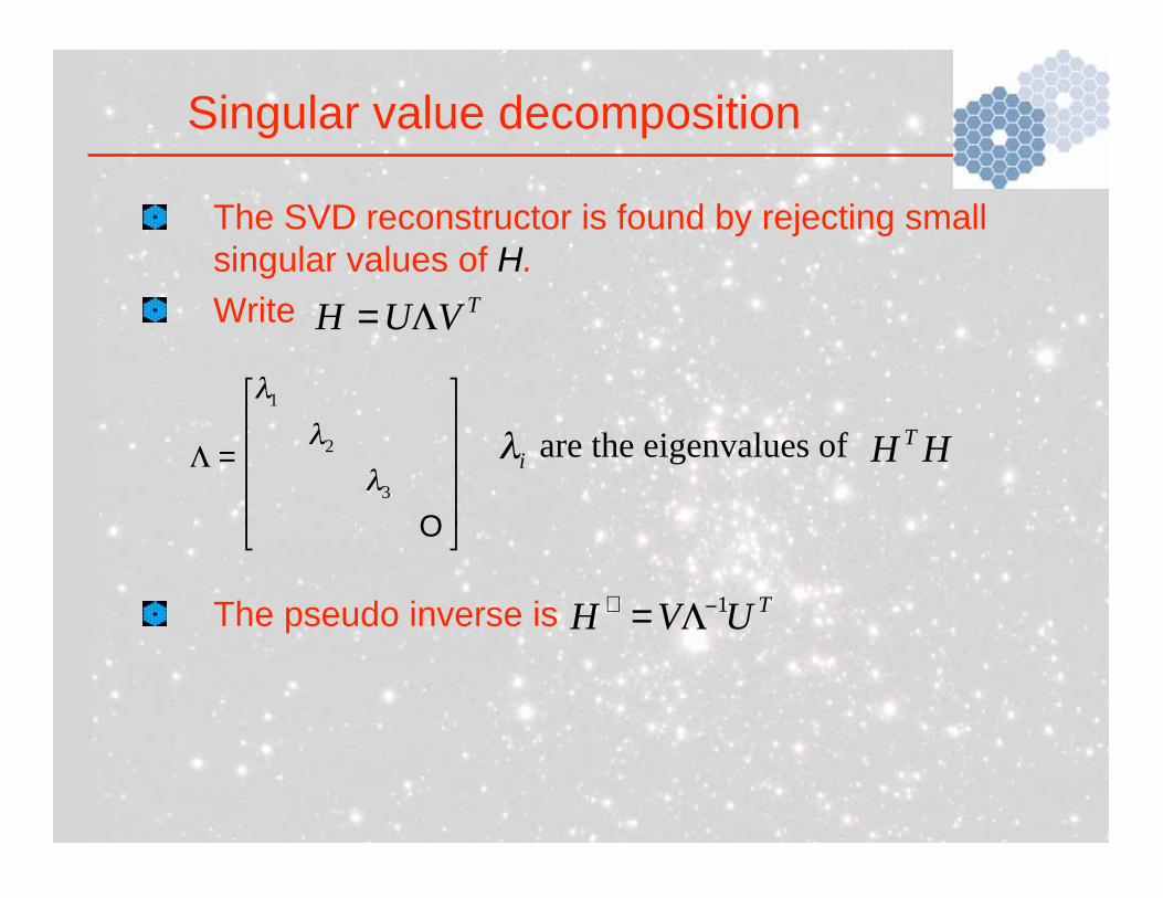
The SVD reconstructor is found by rejecting small
singular values of H.
Write
The pseudo inverse is
Singular value decomposition
TVUH =
=
O
3
2
1
are the eigenvalues of HHT
i
TUVH
1+=
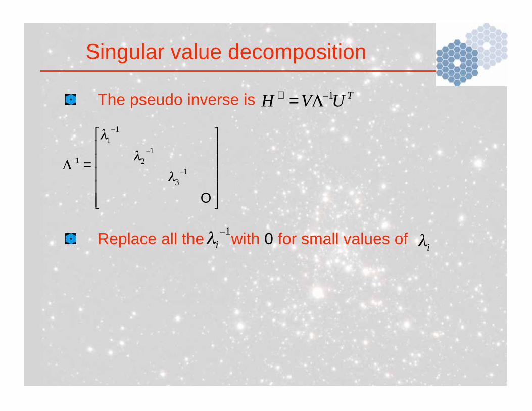
The pseudo inverse is
Replace all the with 0 for small values of
Singular value decomposition
=
O
1
3
1
2
1
1
1
1
i
TUVH
1+=
i
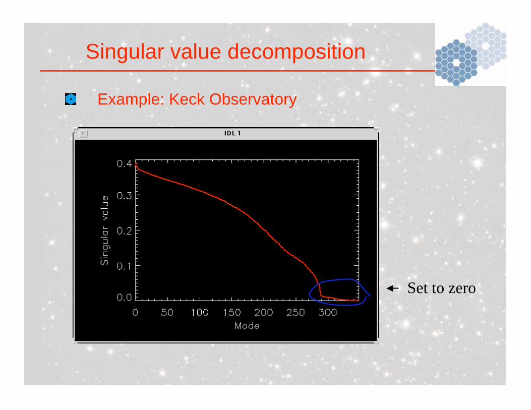
Example: Keck Observatory
Singular value decomposition
Set to zero
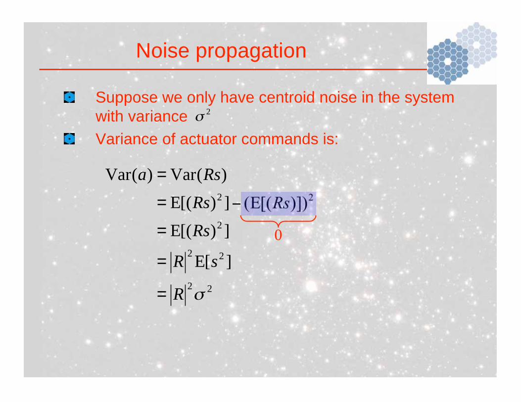
Suppose we only have centroid noise in the system
with variance
Variance of actuator commands is:
Noise propagation
2
22
22
2
22
][E
])[(E
)])[(E(])[(E
)(Var)(Var
R
sR
Rs
RsRs
Rsa
=
=
=
=
=
0
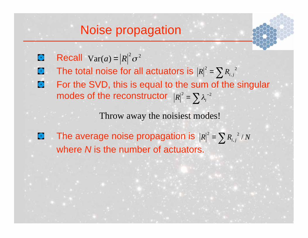
Recall
The total noise for all actuators is
For the SVD, this is equal to the sum of the singular
modes of the reconstructor
The average noise propagation is
where N is the number of actuators.
Noise propagation
22)(Var Ra =
=2
,
2
jiRR
NRR ji /2
,
2=
=22
iR
Throw away the noisiest modes!
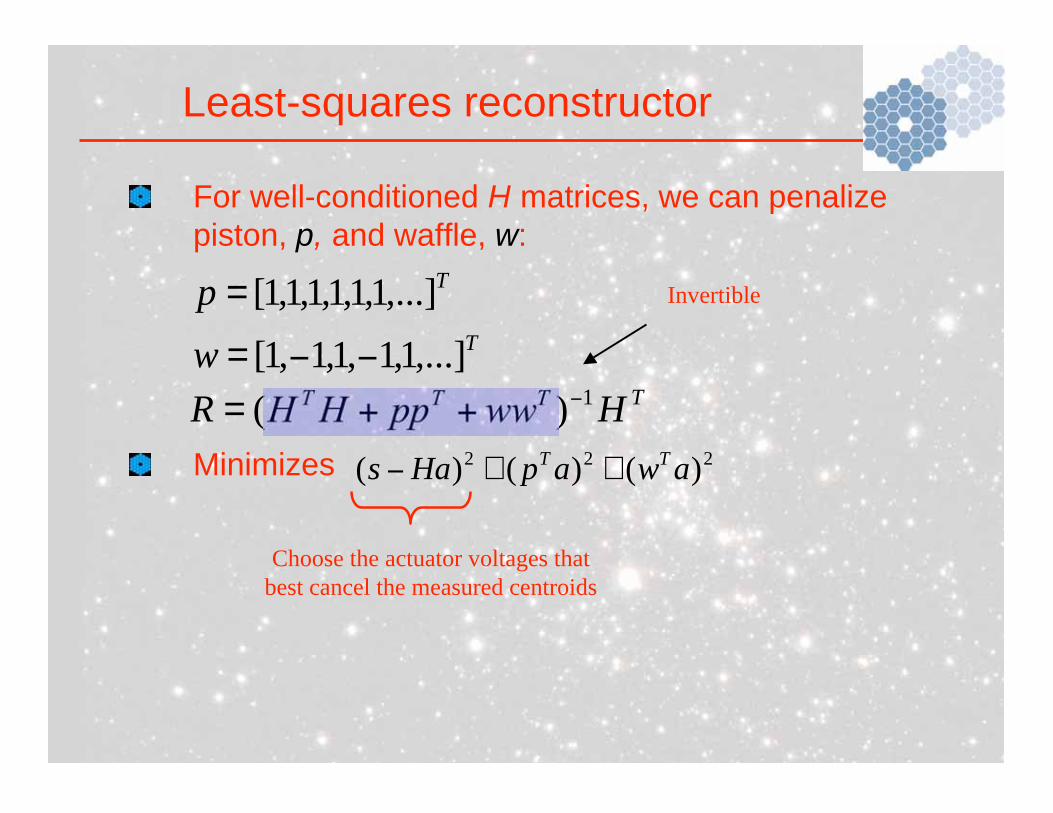
For well-conditioned H matrices, we can penalize
piston, p, and waffle, w:
Minimizes
Least-squares reconstructor
222 )()()( awapHasTT
++
TTTTHwwppHHR
1)( ++=
T
T
w
p
,...]1,1,1,1,1[
,...]1,1,1,1,1,1[
=
=
Choose the actuator voltages thatbest cancel the measured centroids
Invertible
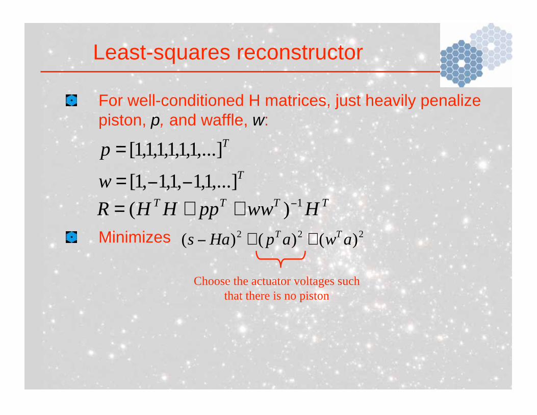
For well-conditioned H matrices, just heavily penalize
piston, p, and waffle, w:
Minimizes
Least-squares reconstructor
222 )()()( awapHasTT
++
TTTTHwwppHHR
1)( ++=
T
T
w
p
,...]1,1,1,1,1[
,...]1,1,1,1,1,1[
=
=
Choose the actuator voltages suchthat there is no piston
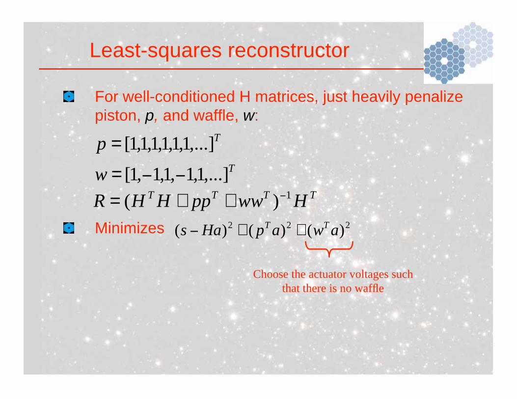
For well-conditioned H matrices, just heavily penalize
piston, p, and waffle, w:
Minimizes
Least-squares reconstructor
222 )()()( awapHasTT
++
TTTTHwwppHHR
1)( ++=
T
T
w
p
,...]1,1,1,1,1[
,...]1,1,1,1,1,1[
=
=
Choose the actuator voltages suchthat there is no waffle
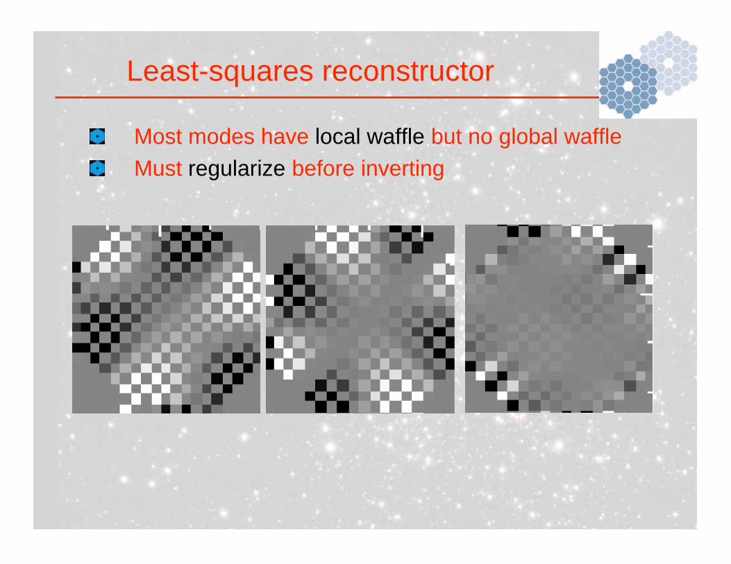
Most modes have local waffle but no global waffle
Must regularize before inverting
Least-squares reconstructor
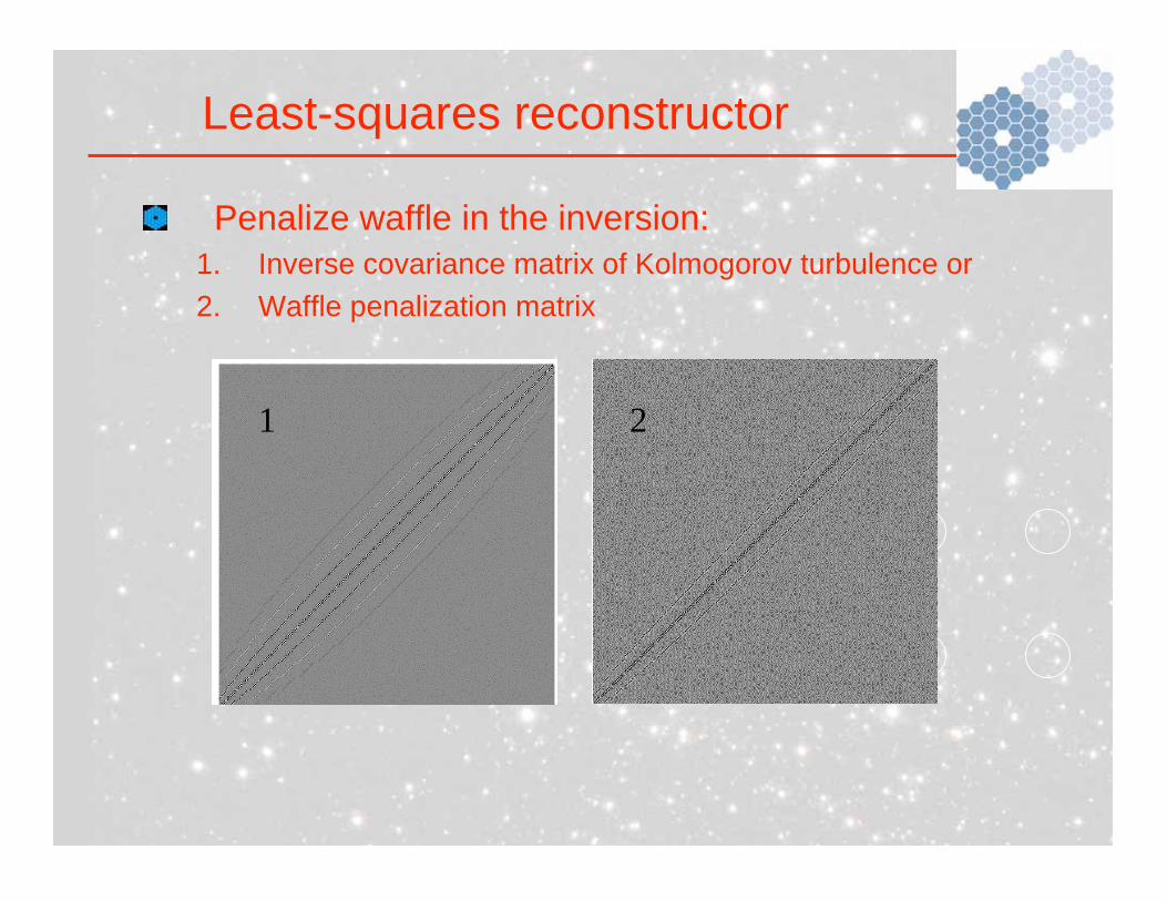
Penalize waffle in the inversion:
1. Inverse covariance matrix of Kolmogorov turbulence or
2. Waffle penalization matrix
Least-squares reconstructor
1 2
Least-squares reconstructor
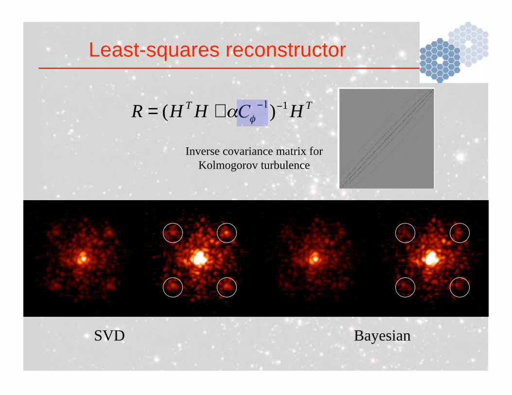
TTHCHHR
11)( +=
SVD Bayesian
Inverse covariance matrix forKolmogorov turbulence
Least-squares reconstructor
TTHCHHR
11)( +=
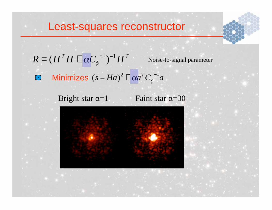
Bright star =1 Faint star =30
Noise-to-signal parameter
aCaHasT 12)( +Minimizes
SVD Bayesian
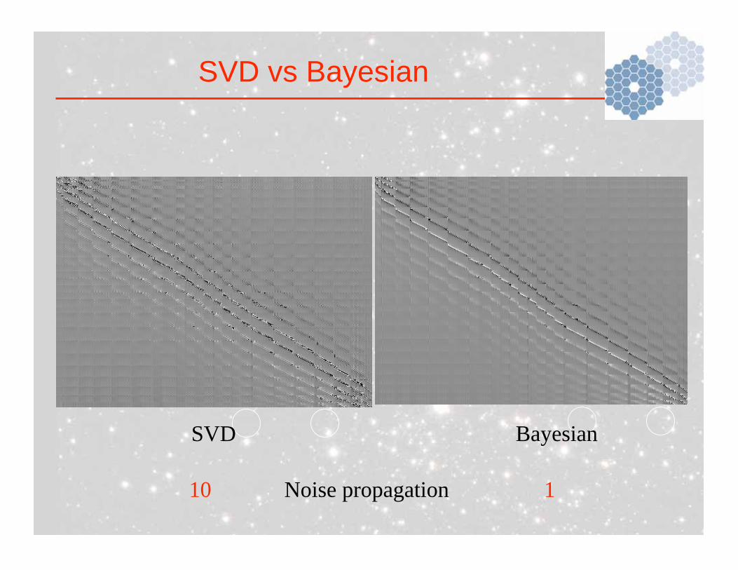
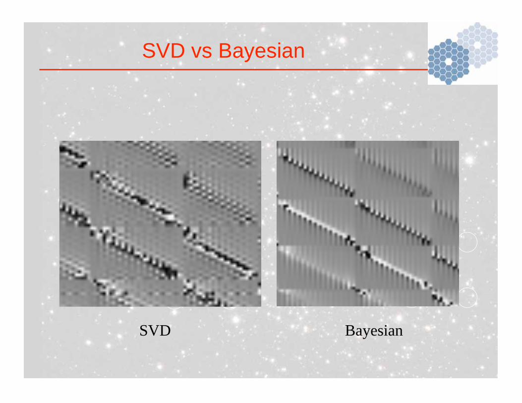
SVD vs Bayesian
10 Noise propagation 1
SVD Bayesian
SVD vs Bayesian
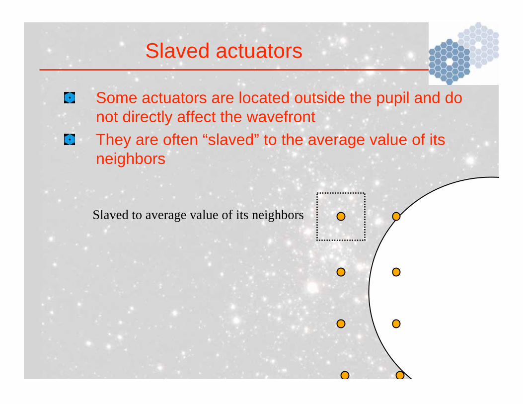
Slaved actuators
Some actuators are located outside the pupil and do
not directly affect the wavefront
They are often “slaved” to the average value of its
neighbors
Slaved to average value of its neighbors
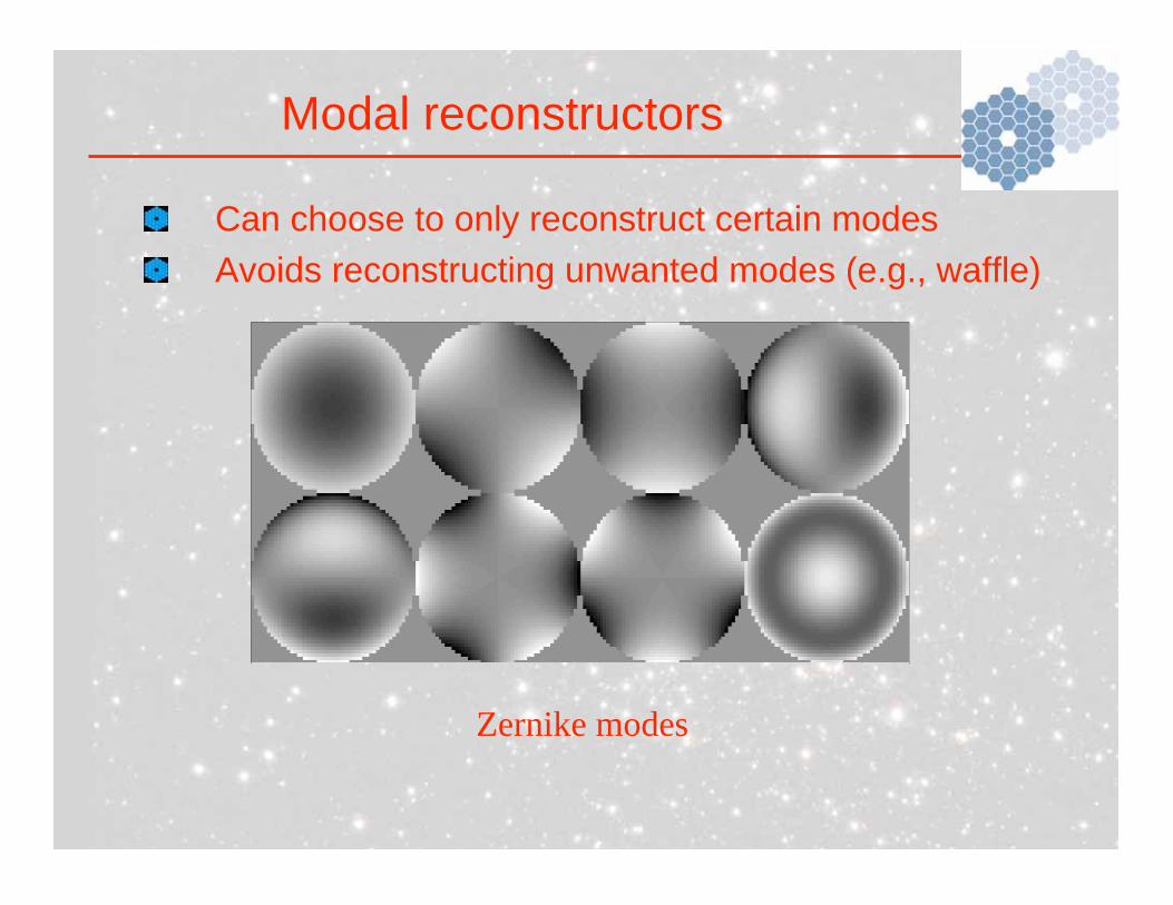
Modal reconstructors
Can choose to only reconstruct certain modes
Avoids reconstructing unwanted modes (e.g., waffle)
Zernike modes
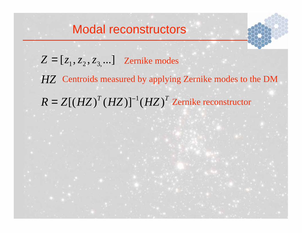
TTHZHZHZZR )()]()[( 1
=
...],,[ ,321 zzzZ =
Modal reconstructors
Zernike modes
HZ Centroids measured by applying Zernike modes to the DM
Zernike reconstructor
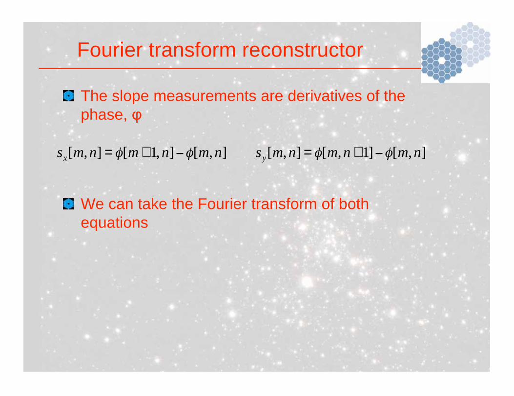
The slope measurements are derivatives of the
phase,
We can take the Fourier transform of both
equations
],[],1[],[ nmnmnmsx
+=
Fourier transform reconstructor
],[]1,[],[ nmnmnmsy
+=
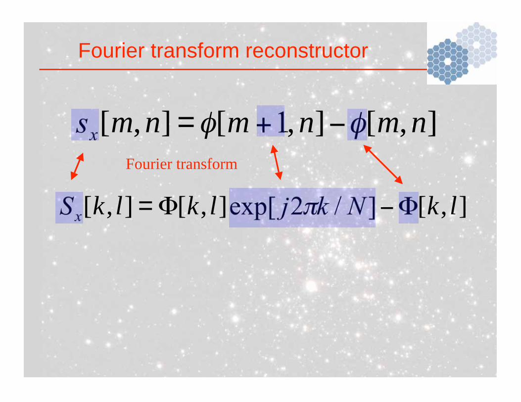
],[],1[],[ nmnmnmsx
+=
Fourier transform reconstructor
],[]/2exp[],[],[ lkNkjlklkSx =
Fourier transform
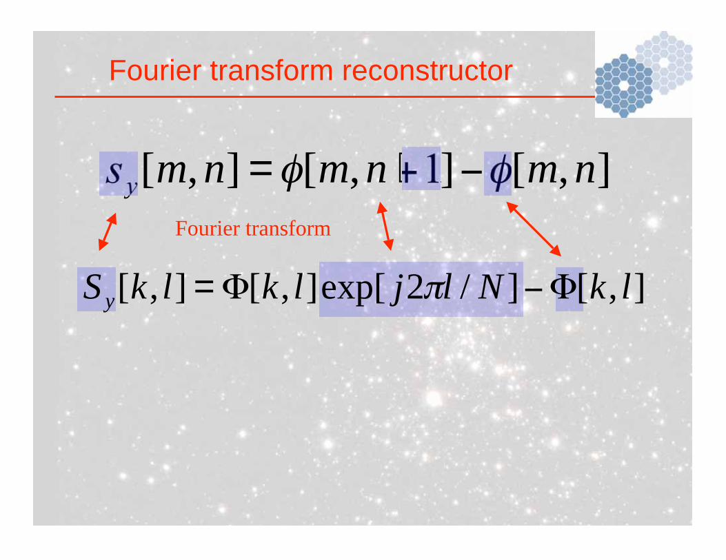
],[]1,[],[ nmnmnmsy
+=
Fourier transform reconstructor
Fourier transform
],[]/2exp[],[],[ lkNljlklkSy =
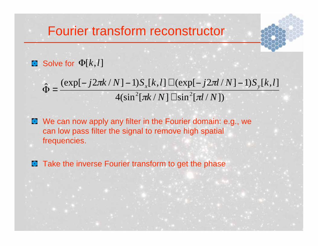
Fourier transform reconstructor
],[ lkSolve for
We can now apply any filter in the Fourier domain: e.g., we
can low pass filter the signal to remove high spatial
frequencies.
Take the inverse Fourier transform to get the phase
])/[sin]/[(sin4
],[)1]/2(exp[],[)1]/2(exp[ˆ
22 NlNk
lkSNljlkSNkj yx
+
+=
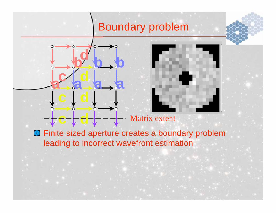
Boundary problem
Finite sized aperture creates a boundary problem
leading to incorrect wavefront estimation
ba
dccc
ddd
b ba aa
Matrix extent
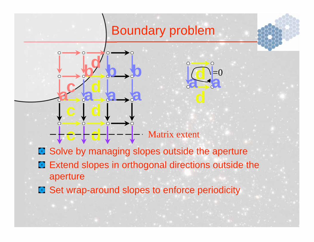
Boundary problem
Solve by managing slopes outside the aperture
Extend slopes in orthogonal directions outside the
aperture
Set wrap-around slopes to enforce periodicity
ba
dccc
ddd
b ba aa
Matrix extent
dd
aa=0
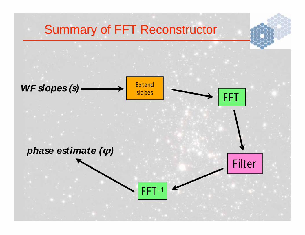
FFT
FFT-1
Filter
ExtendslopesWF slopes (s)
phase estimate ( )
Summary of FFT Reconstructor
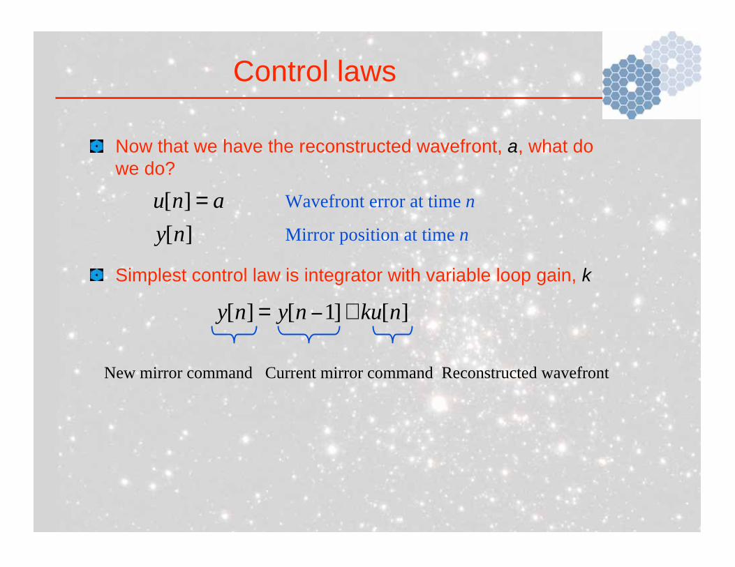
Control laws
Now that we have the reconstructed wavefront, a, what do
we do?
Simplest control law is integrator with variable loop gain, k
][]1[][ nkunyny +=
anu =][
][ny
Wavefront error at time n
Mirror position at time n
New mirror command Current mirror command Reconstructed wavefront
Control laws
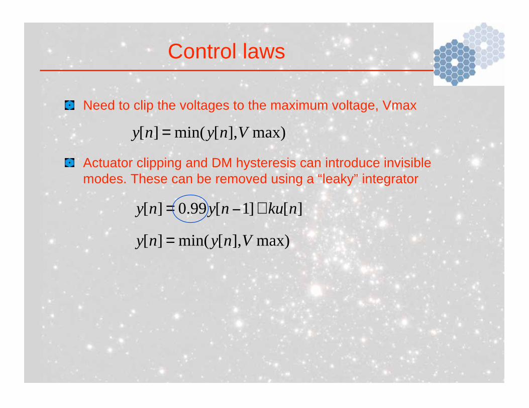
Need to clip the voltages to the maximum voltage, Vmax
Actuator clipping and DM hysteresis can introduce invisible
modes. These can be removed using a “leaky” integrator
max)],[min(][ Vnyny =
][]1[99.0][ nkunyny +=
max)],[min(][ Vnyny =
Control laws
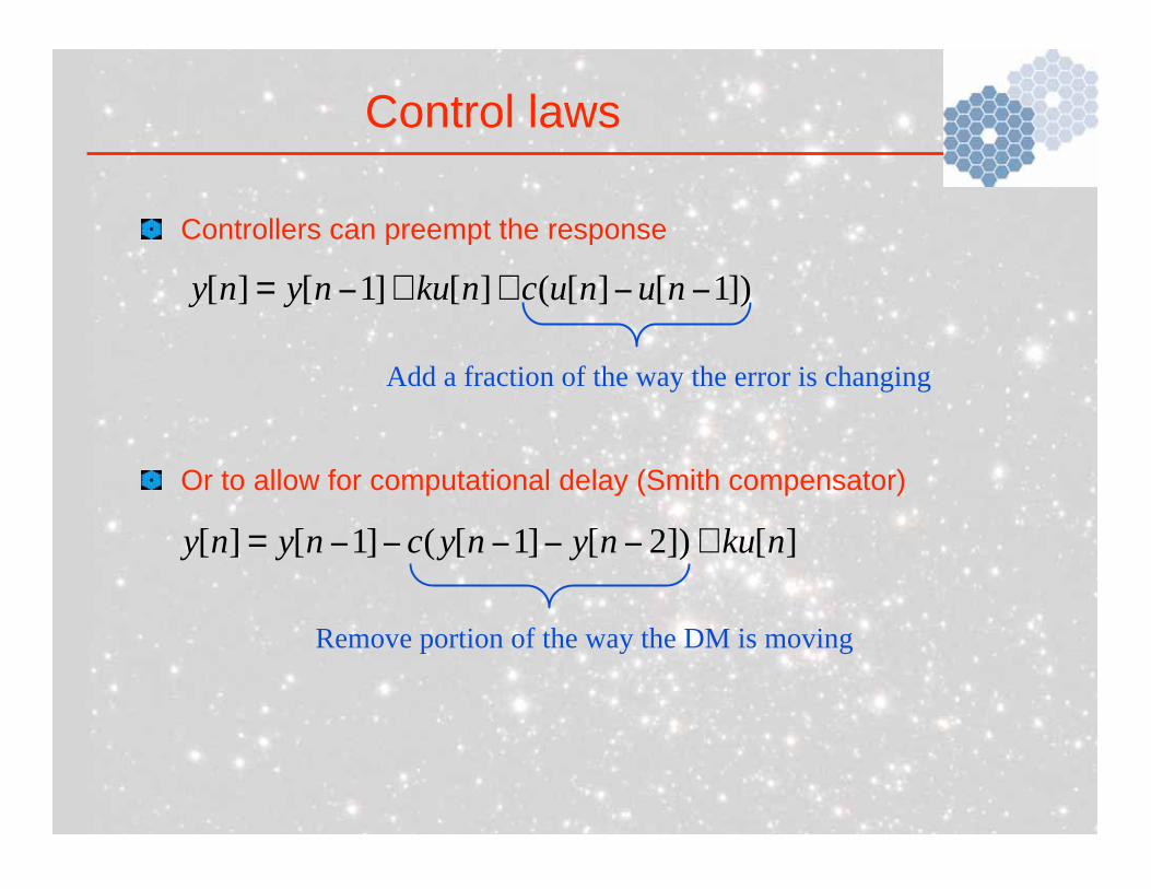
Controllers can preempt the response
Or to allow for computational delay (Smith compensator)
])1[][(][]1[][ ++= nunucnkunyny
][])2[]1[(]1[][ nkunynycnyny +=
Add a fraction of the way the error is changing
Remove portion of the way the DM is moving
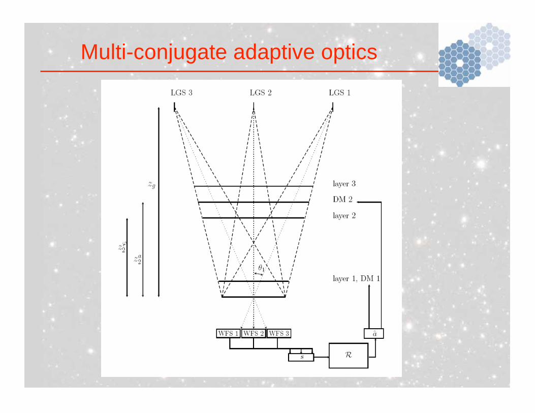
Multi-conjugate adaptive optics
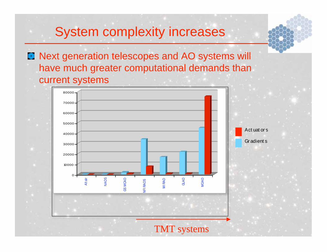
System complexity increases
0
10000
20000
30000
40000
50000
60000
70000
80000
Alt
air
NA
OS
GS
MCA
O
NFIR
AO
S
MIR
AO
GLA
O
MO
AO
TMT systems
Actuators
Gradients
Next generation telescopes and AO systems will
have much greater computational demands than
current systems
Computationally efficient reconstructors
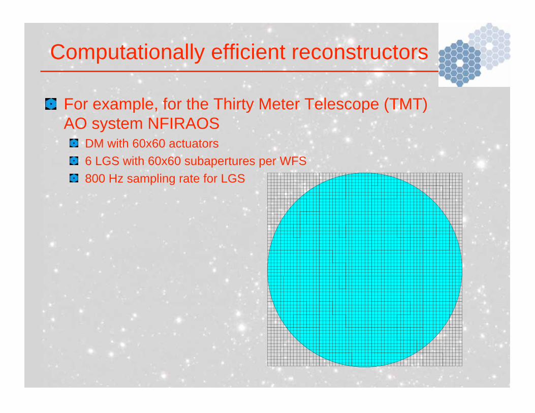
For example, for the Thirty Meter Telescope (TMT)
AO system NFIRAOSDM with 60x60 actuators
6 LGS with 60x60 subapertures per WFS
800 Hz sampling rate for LGS
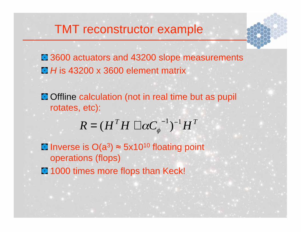
3600 actuators and 43200 slope measurements
H is 43200 x 3600 element matrix
Offline calculation (not in real time but as pupil
rotates, etc):
Inverse is O(a3) 5x10¹⁰ floating point
operations (flops)
1000 times more flops than Keck!
TMT reconstructor example
TTHCHHR
11)( +=
TMT reconstructor example
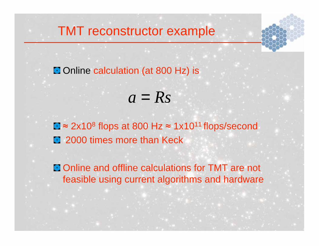
Online calculation (at 800 Hz) is
2x10⁸ flops at 800 Hz 1x10¹¹ flops/second
2000 times more than Keck
Online and offline calculations for TMT are not
feasible using current algorithms and hardware
Rsa =

Now for the good stuff!
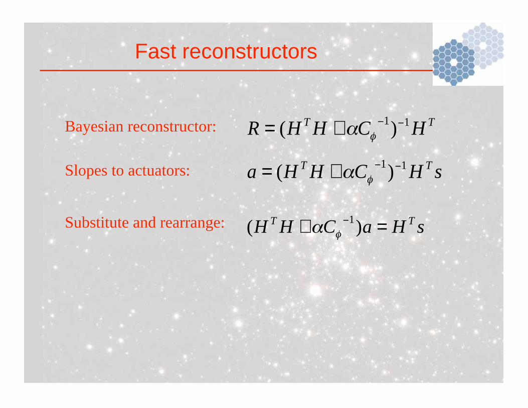
Fast reconstructors
TTHCHHR
11)( +=
sHaCHHTT
=+ )(1
Bayesian reconstructor:
Slopes to actuators:
Substitute and rearrange:
sHCHHaTT 11
)( +=
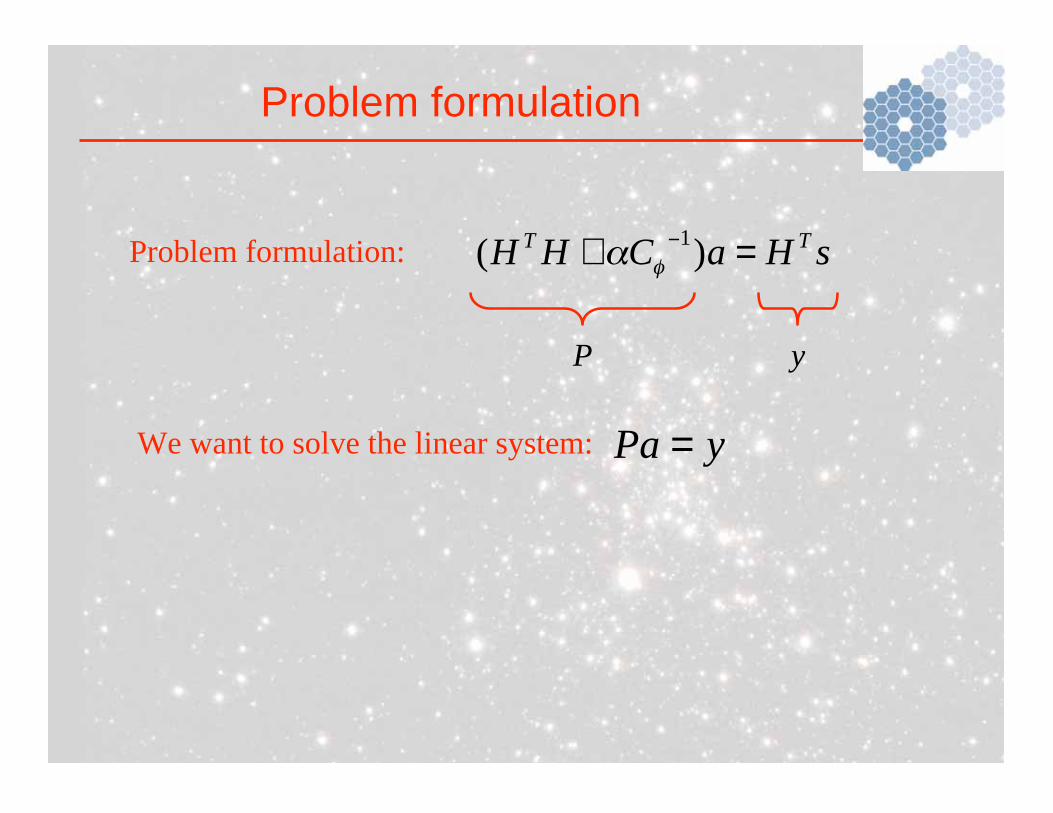
Problem formulation
sHaCHHTT
=+ )(1Problem formulation:
yPa =We want to solve the linear system:
P y
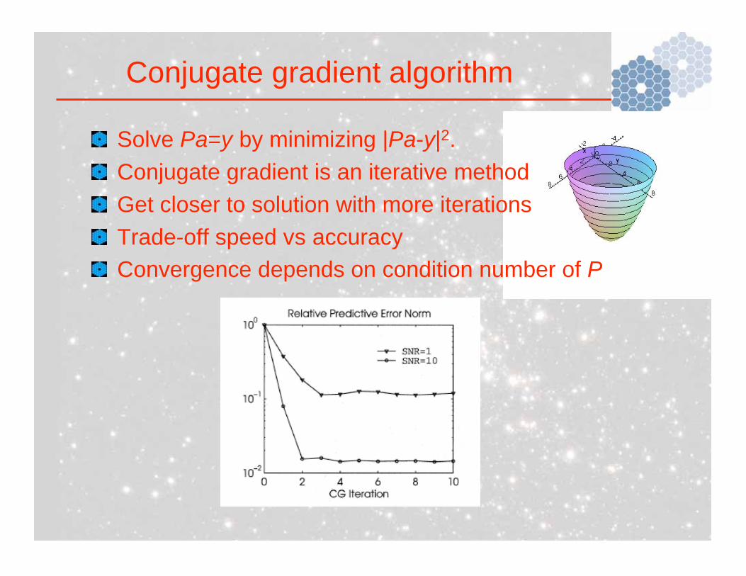
Conjugate gradient algorithm
Solve Pa=y by minimizing |Pa-y|2.
Conjugate gradient is an iterative method
Get closer to solution with more iterations
Trade-off speed vs accuracy
Convergence depends on condition number of P
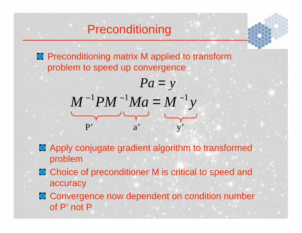
Preconditioning
Preconditioning matrix M applied to transform
problem to speed up convergence
yMMaPMM111
=
Apply conjugate gradient algorithm to transformed
problem
Choice of preconditioner M is critical to speed and
accuracy
Convergence now dependent on condition number
of P’ not P
P’ a’ y’
yPa =
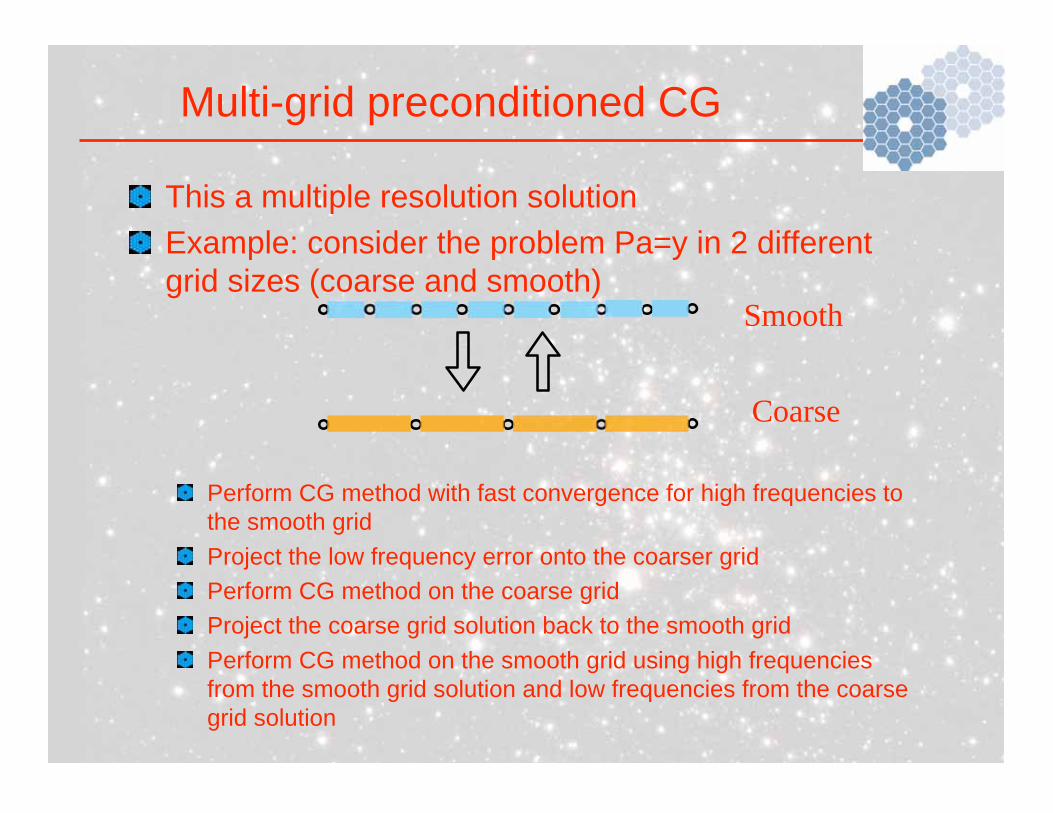
Multi-grid preconditioned CG
This a multiple resolution solution
Example: consider the problem Pa=y in 2 different
grid sizes (coarse and smooth)
Perform CG method with fast convergence for high frequencies to
the smooth grid
Project the low frequency error onto the coarser grid
Perform CG method on the coarse grid
Project the coarse grid solution back to the smooth grid
Perform CG method on the smooth grid using high frequencies
from the smooth grid solution and low frequencies from the coarse
grid solution
Smooth
Coarse
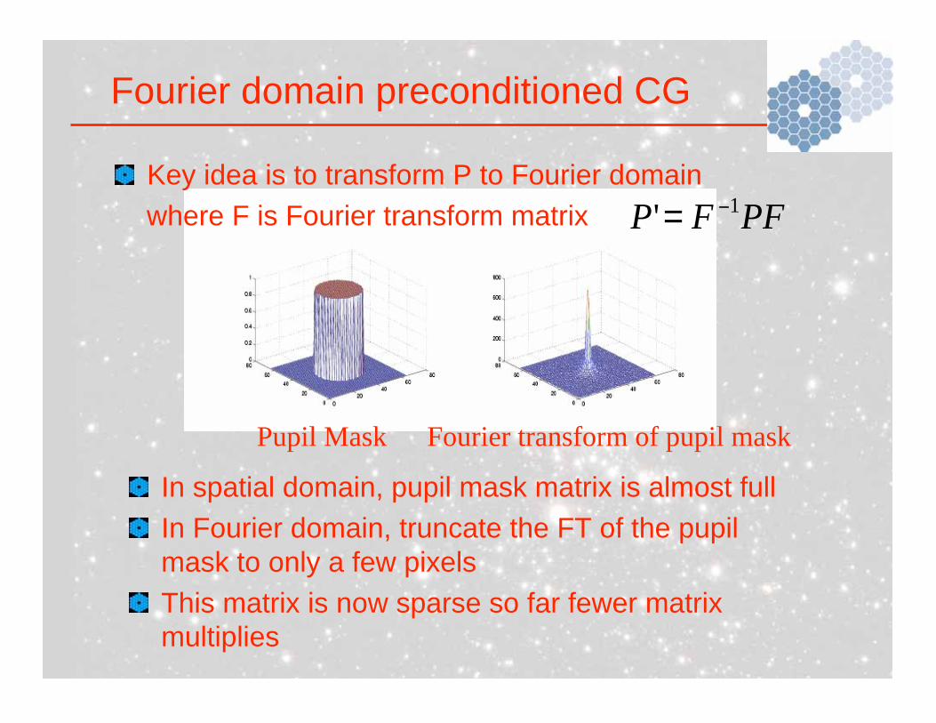
Fourier domain preconditioned CG
Key idea is to transform P to Fourier domain
where F is Fourier transform matrix PFFP1
'=
Pupil Mask Fourier transform of pupil mask
In spatial domain, pupil mask matrix is almost full
In Fourier domain, truncate the FT of the pupil
mask to only a few pixels
This matrix is now sparse so far fewer matrix
multiplies
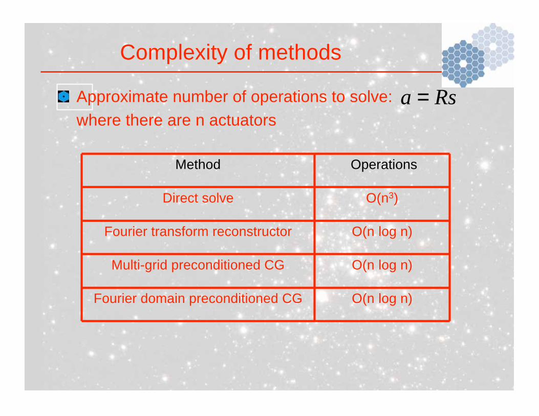
Complexity of methods
O(n log n)Fourier domain preconditioned CG
O(n log n)Multi-grid preconditioned CG
O(n log n)Fourier transform reconstructor
O(n3)Direct solve
OperationsMethod
Rsa =Approximate number of operations to solve:
where there are n actuators
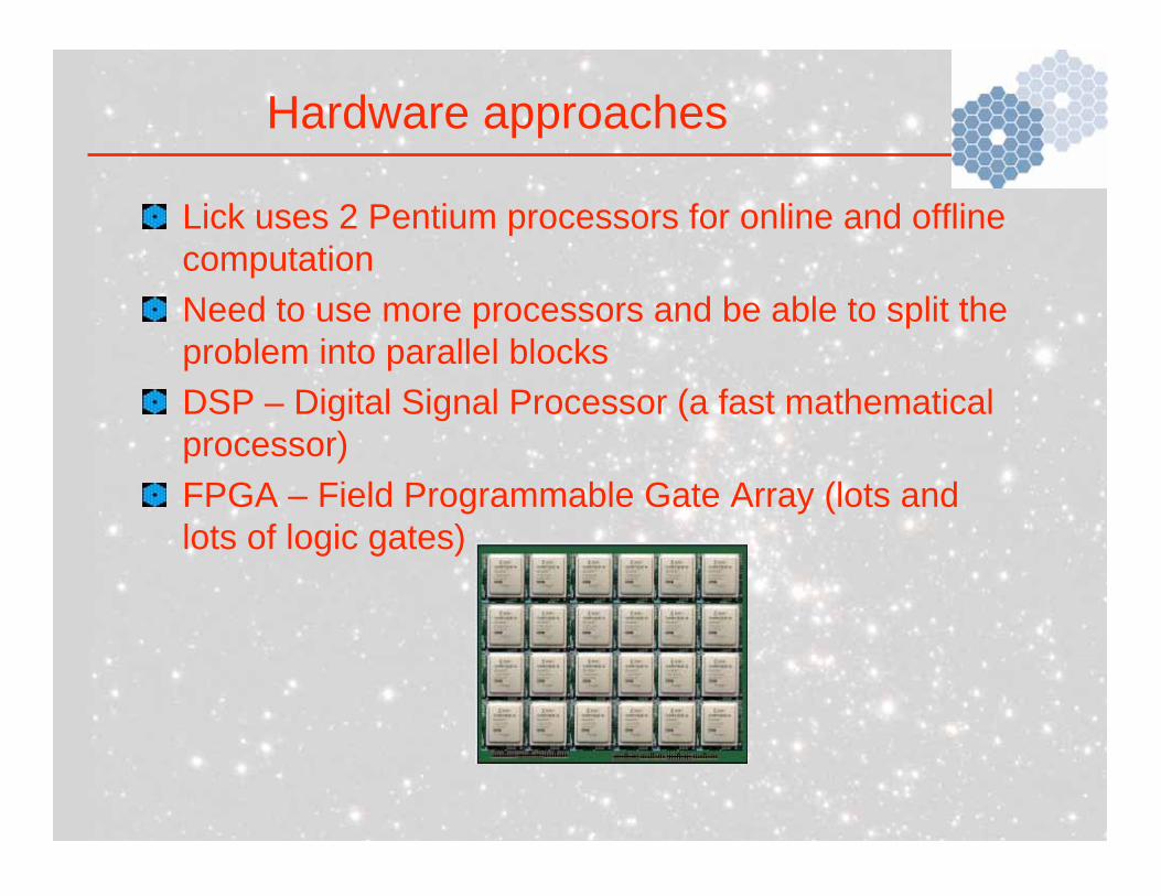
Hardware approaches
Lick uses 2 Pentium processors for online and offline
computation
Need to use more processors and be able to split the
problem into parallel blocks
DSP – Digital Signal Processor (a fast mathematical
processor)
FPGA – Field Programmable Gate Array (lots and
lots of logic gates)

Hardware approach for TMT
Proposed TMT hardware solution is to use
combination of FPGAs and DSPs
DSP does pixel processing (centroiding etc)
FPGAs do tomography and fitting steps
•FPGA •FPGA
•FPGA •FPGA
•FPGA •FPGA •FPGA
•DSP
•FPGA
Mahalo!