Wavefront correction through image sharpness maximisation

L. P. Murray∗, J. C. Dainty and L. Daly

Applied Optics Group, Department of Experimental Physics, National University of Ireland, Galway, Ireland.

ABSTRACTA key component of any adaptive optics system (AO) for the correction of wavefront aberrations, is the wavefront sensor(WFS). Many systems operate in a mode where a WFS measures the aberrations present in the incoming beam. Therequired corrections are determined and applied by the wavefront corrector - often a deformable mirror (DM). We wishto develop a wavefront sensor-less correcting system, as derived from the original adaptive optics system of Muller andBuffington[1]. In this experiment we employ a method in which a correcting element with adjustable segments is driven tomaximise some function of the image. We employ search algorithms to find the optimal combination of actuator voltagesto maximise a certain sharpness metric. The “sharpness” is based on intensity measurements taken with a CCD camera.Results have been achieved using a Nelder-Mead variation of the Simplex algorithm[2]. Preliminary results show that theSimplex algorithm can minimise the aberrations and restore the Airy rings of the imaged point source. Good correction isachieved within 50-100 iterations of the Simplex algorithm. The results are repeatable and so-called “blind” correction ofthe aberrations is achieved. The correction achieved using various sharpness algorithms laid out by Muller and Buffingtonare evaluated and presented.

Keywords: Adaptive Optics, Image Sharpness, Simplex Algorithm

1. INTRODUCTIONThe vast area now affected and dependant on adaptive optics stems originally from an AO system proposed by H. Bab-cock[3]. This involved the implementation of a deformable mirror to correct atmospherically degraded stellar images.Before correction can be applied the wavefront aberrations need to be determined. Conventionally, this is done usingwavefront sensors, which measure the phase, phase gradient or phase curvature directly. The necessary commands are thenapplied to the correcting device - usually a deformable mirror - to compensate for phase aberrations[3,4].

1.1. Direct Wavefront SensingThe wavefront sensor is one of the basic elements of conventional adaptive optics systems. It is required to sense thewavefront with high spatial resolution and speed to apply a real time correction. Direct wavefront sensing methods suchas the Shack-Hartmann WFS[3] provide information about the wavefront phase, which is then used drive a wavefrontcorrector. In this sense, direct wavefront sensors directly measure the wavefront phase from which the necessary correctioncan be determined. Indirect wavefront sensing measures the intensity distribution in the image-plane and deduces from thisthe wavefront aberration. Generally, direct methods are employed in atmospheric and vision science AO where correctionsneed to be made at a much higher rate. Indirect methods might be of value in industrial and medical applications becauseof their potential for simplicity.

1.2. Indirect Wavefront SensingIndirect techniques do not directly measure implicit or explicit wavefront properties, but use information related to thewavefront to provide the signal for the corrective element without reconstruction. This area of research is based on a“sharpness” criterion, which is used as an image metric to measure the degree of correction of the wavefront phase. Theprinciple of image sharpening can be explained by figure 1, a schematic diagram of image sharpening methods.

The image sharpness metric is a measure of the image quality and in general the higher this metric the better the imagequality. In sharpness maximisation a trial phase correction is applied to the image via a corrector and the effect on thesharpness metric is noted. Using a suitable sharpness metric, and a search algorithm which determines the trial phase to beapplied to the corrector, the system is driven to maximise the sharpness metric and minimise the aberration.

∗*Further information: (Send correspondence to L. P. M.) E-mail: larry.murray@nuigalway.ie, Telephone +353 91 522428

Control

Block

Image

Quality

Analyzer

Camera

ObjectDistorting

Medium

Transmissive

Wavefront

Corrector

Lens

Figure 1. Basic configuration of image sharpness correction system (after Vorontsov[8])

2. IMAGE SHARPNESS PRINCIPLEThe intensity in the focal plane must be such that the image degraded by some disturbance can be recovered. This requiresmanipulation of the phase correcting elements while observing some sharpness metric of the image. The problem ariseswhen one quantitatively tries to define the word “sharp”. One approach to this was described by Muller and Buffington[1].

Muller and Buffington define the sharpness such that its value for an aberration-degraded image is always less than thatof the true image. In their paper Muller and Buffington set out 8 sharpness metrics, some of which have been proven to bemaximised for various images. One such sharpness definition is

S =∫

I2(x, y)dxdy, (1)

where x, y denote coordinates in the image plane and I(x, y)is the image irradiance. This sharpness definition will bemaximised when there is zero wavefront error, even in the presence of irregular object radiance distribution. This amplitudeinsensitivity makes this method useful for large extended objects. Other sharpness functions, such as higher-order momentsof distribution, or entropy minimization functions,

S = −∫

I(x, y)ln[I(x, y)]dxdy, (2)

have been examined by Muller and Buffington[1] and are proven to relate to low wavefront error.

2.1. Image-plane Sharpness FunctionsThe metric used for image correction could be any real time quantity that indicates system “quality” as affected by wave-front distortion. Depending on the type of adaptive optics system, the performance metric might be intensity of radiationat the focus[5], image sharpness[1], or scattered field statistical moments[6].

Feinup and Miller[7] explored variations of the sharpness metrics proposed by Muller and Buffington and found thatdifferent metrics worked better depending on the type of scene. Power law metrics with larger powers tend to performbetter with scenes having prominent scatters, whereas power-law metrics with smaller powers perform better with sceneshaving no prominent scatters. The original power-law metrics set out by Muller and Buffington are of the form S =∫

In(x, y)dx, dy where n=2,3,4. Feinup and Miller extended their form to include the second derivative of the nonlinearpoint transformation..

They found that the behaviour of a metric is determined by the second derivative of its point nonlinearity as a functionof the image intensity. Its shown both theoretically and experimentally that metrics having similar second derivatives gavesimilar results when used in an image sharpening algorithm. For, example negative Shannon entropy acts in a similar wayto a power law near unity. Metrics whose second derivative increases with increasing intensity emphasise bright points,whereas, metrics whose second derivative decreases with decreasing intensity emphasize making shadows and low returnareas darker. Given these trends it is then possible to specify optimal metrics for particular images.

Vorontsov[8] and Cohen[9] have applied a technique to imaging extended objects. A coherent optical processor is usedin which the signal from the imaging camera is used to control a spatial light modulator (SLM) illuminated by a coherentwavefront. The output from the SLM will then be spatially modulated depending on the camera signal. If this is focusedonto a rotating frosted glass plate a characteristic speckle pattern will be observed. The smaller the speckle scale, the higherthe spatial frequency content of the image. The system is then driven to minimise the speckle size[10].

Several of the sharpness metrics outlined by Muller and Buffington are listed below

S1 =∫

I2(x, y)dx, dy, (3)

as described earlier. This metric has been proven for monochromatic light and is maximised when there is zero apertureplane distortion. This is proved using a version of the Fresnel-Kirchoff equation to calculate the irradiance. S1is maximisedfor zero distortion irrespective of the object-irradiance distribution[1].

Another sharpness metric is,

S2 = I(x0, y0), (4)

where the irradiance of the image at an arbitrary point (x0, y0) on the image plane. Muller and Buffington suggest thatobjects that have a brightest spot S2will be maximised when the image of that bright spot is shifted over the point (x0, y0).

A sharpness metric used in a system described by O’ Meara[11,12] is,

S3 =∫|I(x, y)M(x, y)| dxdy, (5)

where M(x, y)is a mask function. If M is an accurate replica of the true undistorted image, then S3is a good sharpnessdefinition[1].

As described earlier, the power-law metrics can be used as a measure of image quality,

S4 =∫

In(x, y)dxdy, (6)

where n=2,3,4.

A commonly employed sharpness metric, often known as “power in the bucket” is given by,

S5 =∫

A

I dxdy, (7)

which is an integral of the intensity in some region A of the image space - often a central disc or the maximisation ofthe amount of light passing through a pin hole.

The choice of the sharpness metric depends upon the object. S3 has been shown to work well for point objects evenfor cases where the mask, M, only approximately matches the undisturbed image. For example M can be a pinhole whichhas a diameter equal to the diffraction limited image. However this metric would not work as well for extended objects asa priori information about the object would be required, whereas, S1 is expected to work better for extended objects[13].

3. SEARCH ALGORITHMSImage sharpness maximisation requires the correcting device to be driven to its optimal shape to minimise the aberra-tions. For a DM with 37 actuators which operate over 255 different voltages this is an unfeasibly large space to searchsystematically. To search the large range of possible mirror shapes (25537degrees of freedom (DOF)) it is necessary to im-plement a search algorithm to determine the global minimum. One of the most effective and widely used multidimensionaloptimisation search methods is the Simplex method - which is described below.

Ideally when using a search algorithm routine the global minimum is the final state i.e. the true minimum of the system.this is very difficult to find for systems having a large number of DOF, the probability of falling into a local minimum.Generally, for complicated optimisation problems, non-systematic search routines will give the best solution[13].

3.1. The Nelder-Mead Simplex AlgorithmThe simplex search method proposed by Nelder and Mead[14] is an algorithm that tries to minimise a scalar-valuednonlinear function of n real variables using only function values. A simplex is a geometrical figure consisting of n + 1vertices, where n is the number of DOF. In two dimensions a simplex would be a triangle, in three, a tetrahedron and inthis experiment a complex figure with 38 vertices. Each vertex represents a set of mirror voltages. Initially, 38 (n + 1)random sets of voltages are generated and the corresponding sharpness value is measured for each vertex. Based on theinitial evaluations the simplex attempts to adapt to the local landscape, with the aim of contracting to the global minimum.This is done through a series of reflections, expansions, contractions and shrink operations. The simplex can be set to runfor a certain number of iterations, or to stop when a termination criteria is met.

Although Nelder and Mead published their paper in 1965, no theoretical results regarding convergence properties of theNelder-Mead method in higher dimensions have yet been proven. Even finding any function in R2 for which the algorithmwould always converge to a minimum still remains and open problem[15]. Therefore, one cannot say with certainty thatthe maximum sharpness value reached by the simplex is the global maximum.

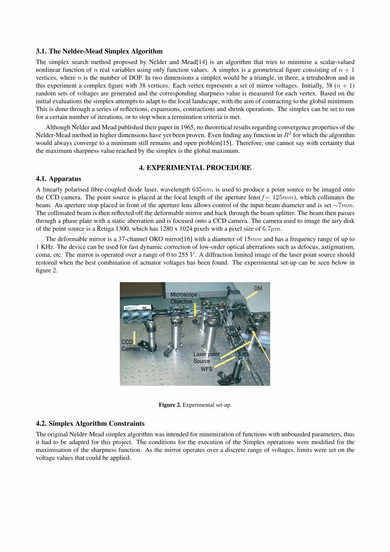
4. EXPERIMENTAL PROCEDURE4.1. ApparatusA linearly polarised fibre-coupled diode laser, wavelength 635nm, is used to produce a point source to be imaged ontothe CCD camera. The point source is placed at the focal length of the aperture lens(f= 125mm), which collimates thebeam. An aperture stop placed in front of the aperture lens allows control of the input beam diameter and is set ∼7mm.The collimated beam is then reflected off the deformable mirror and back through the beam splitter. The beam then passesthrough a phase plate with a static aberration and is focused onto a CCD camera. The camera used to image the airy diskof the point source is a Retiga 1300, which has 1280 x 1024 pixels with a pixel size of 6.7µm.

The deformable mirror is a 37-channel OKO mirror[16] with a diameter of 15mm and has a frequency range of up to1 KHz. The device can be used for fast dynamic correction of low-order optical aberrations such as defocus, astigmatism,coma, etc. The mirror is operated over a range of 0 to 255 V . A diffraction limited image of the laser point source shouldrestored when the best combination of actuator voltages has been found. The experimental set-up can be seen below infigure 2.

CCD

Camera

WFS

DMMicroscope

Objective

Laser point

Source

Figure 2. Experimental set-up.

4.2. Simplex Algorithm ConstraintsThe original Nelder-Mead simplex algorithm was intended for minimization of functions with unbounded parameters, thusit had to be adapted for this project. The conditions for the execution of the Simplex operations were modified for themaximisation of the sharpness function. As the mirror operates over a discrete range of voltages, limits were set on thevoltage values that could be applied.

The termination criteria proposed by Nelder and Mead were used to restart the optimisation procedure with a newsimplex, where all vertices’s except for the ”best” point are randomly re-generated. This method is intended to prevent thesimplex from shrinking to a false minimum.

4.3. Experimental ProcessWith the experimental set-up described above, the power law metrics (eq:6) described by Muller and Buffington wereexamined. Each metric was evaluated for 50 and 100 iterations of the Simplex algorithm and their sharpness values andimprovement in strehl ratio compared. The static plates used to implement the aberrations are relatively weak plates withnominally 0.25λ of defocus and astigmatism and with other distortions present of small amounts. The static aberrationinduced consists a of defocus and an astigmatism plate superimposed to increase the magnitude of the aberration. Theaberrations were produced through a photo-induced refractive index change on Foturan photosensitive glass[17]. Aninterferometric image of the refractive index change for a defocus plate can be seen below in figure 3.

Figure 3. Example of aberration induced by defocus plate.

5. RESULTSThe Simplex algorithm was used to correct for aberrations introduced into the image of the point source. The algorithmwas run for I2, I3, I4for 50 and 100 algorithms. For each power-law sharpness definition, 100 iterations of the algorithmwas run. It was seen that for each case the algorithm converged to a maximum before 50 iterations so future correctionswere limited to 50 iterations. An example of the convergence of I3 below 50 iterations can be seen below in figure 4.

Sharpness Value for I3 - 100 Iterations

1.00E-09

1.10E-09

1.20E-09

1.30E-09

1.40E-09

1.50E-09

1.60E-09

1.70E-09

1.80E-09

1.90E-09

0 20 40 60 80 100Iteration Number

Sharp

ness V

alu

e (

Dig

ital U

nits)

Figure 4. Convergence of I3to a maximum.

Each power-law metric achieved a similar increase in the comparative Strehl ratio of the image. The comparative Strehlwas taken to be factor by which the intensity density of the central maximum increased when the correction algorithm wasapplied. A mask was applied around the maximum intensity region and the average intensity was taken. This average forthe corrected image was divided by the uncorrected average to get the factor of improvement.

The algorithm ran the fastest for the I3 sharpness metric as the algorithm was less likely to perform shrink operations,whereby, each vertex of the simplex (38) is shrunk and re-evaluated within one iteration. Often 50 iterations would takeapproximately 2 mins compared to approximately 20 mins for I2 and ~ 30 mins of I4. However, the limiting factor for thecorrection time for each algorithm was not connected to the nature of the sharpness metrics. The limiting factor was theprocessing of the image TIF files. Each image was read from the camera, stored and then re-read for processing. To speedthe correction time, a faster method of processing the TIF files directly from the camera would be beneficial.

As mentioned before the algorithm would reach a maximum sharpness value in less than 50 iterations and this can beseen (figure 5) in a sample of some algorithm runs for I2. Each iteration reaches a “maximum” value which correspondsto a restored image. The difference in the final sharpness value may be due to shot noise in the CCD read out or perhaps alocal maximum.

Sharpness Value vs Iteration Number for I2

1.56E-05

1.58E-05

1.60E-05

1.62E-05

1.64E-05

1.66E-05

1.68E-05

1.70E-05

1.72E-05

1.74E-05

0 10 20 30 40 50

Iteration Number

Sh

arp

ne

ss V

alu

e (

Dig

ita

l

Un

its)

Figure 5. Sharpness value vs Iteration number for I2

The increase in the Strehl of the aberrated point source achieved using I4 as a sharpness definition and with 50 iterationscan be seen below in figure 6. As can be seen this metric improves the image intensity significantly.

Profile of Corrected and Uncorrected Image for I4

0

500

1000

1500

2000

2500

3000

3500

4000

30 40 50 60 70 80Pixel Number

Inte

nsity

(D

igita

l Units

)

corrected

Uncorrected

Figure 6. Image profile of corrected and uncorrected image for I4

Comparision of Profile of Corrected Images

0

500

1000

1500

2000

2500

3000

3500

4000

30 40 50 60 70 80Pixel Number

Inte

nsity

(D

igita

l Units

) I2

I3

I4

Figure 7. Comparison of corrected image profile for I2,I3and I4

The correction achieved by the three power-law metrics is compared in figure 7. It can be seen that each metric producesa similar result after 50 iterations.

The maximum intensity of each image was increased for each image metric. The I2sharpness metric increased thecentral pixel intensity by a factor of 1.36 ± 0.07, for metric I3this factor was 1.39 ± 0.07 and for metric I4, 1.30 ± 0.09.

A comparison can be seen in figure 8 between an aberrated image and the correction achieved after 50 iterations of thesimplex algorithm with the power-law I2 as the sharpness metric.

50 Iterations of Simplex

Uncorrected Image Corrected Image

Results acheived after 50

iterations of the simplex

algorithm. As can be seen

from the images the airy

rings of the point source

have been restored.

Images are displayed on

a log scale.

Figure 8. Aberrated and corrected point source image.

ACKNOWLEDGMENTSThis research is funded by Science Foundation Ireland under grant nu

6. CONCLUSIONSThe power-law metrics set out by Muller and Buffington have been shown to produce good correction for a point sourceimage. The Strehl factor improvement achieved by image sharpness metrics I2, I3 and I4 is comparable. For each metricthe maximum sharpness value corresponded to an increase in the images intensity in the central core. This is evidence thatthe image quality can be improved by maximising its sharpness. The simplex algorithm has been shown to determine a

maximum sharpness value for each image metric. The simplex algorithm ran fastest for I3, often achieving good correctionin approximately 2 mins, whereas the I2 and I4 algorithms took significantly longer. This may be that the search spacecorresponding to each metric is different and the I3 metric search space has less local minima. A consequence for thesimplex upon falling into a local minimum is to continuously perform shrink operations in an attempt to close in on theminimum. This is time consuming and its is better for the simplex to reach the minimum through single step iterationssuch as reflections and expansions. The simplex algorithm preforms many more time consuming “shrink” operations forsharpness metrics I2and I4. This may be due to their search space. Nevertheless each metric achieved a significant increasein the image quality. Each metric was seen to reach a plateau in terms of sharpness value and would not increase no matterhow many iterations are performed. This is a measure of the level of correction achieved as, from inspection, the maximumsharpness was effectively reached - at least to the degree which the mirror shape can produce as this is of course limited.Each final image corresponding to 50 iterations and an maximum sharpness was a clear point source with its airy ringsrestored.

It has been shown that the power-law metrics can be used to “blindly” correct for small aberrations in an indirect wave-front sensing system, or, act as a wavefront-sensor less correction. These measurements have been made in monochromaticlight and the metric have been seen to correct for an aberrated point source image. The next trial of these metrics would beto test them on extended objects and to broaden the spectrum of imaging light.

ACKNOWLEDGEMENTSThis research is funded by Science Foundation Ireland under grant number SFI/01/PL2/B039C and by HP Laboratories.

REFERENCES1. R. A. Muller and A. Buffington, “Real-time correction of atmospherically degraded telescope images through image

sharpening”, J Opt. Soc. Am. 67, 1200-1210 (1974).2. J. A. Nelder and R. Mead. “A simplex method for function minimisation” Computer Journal, 7:308, 1965.3. R. K. Tyson, “Principles of Adaptive Optics”, Academic Press, 2nd Edition, 1998.4. J. W. Hardy, “Adaptive Optics for Astronomical Telescopes”, Oxford University Press, 1998.5. H. W. Babcock, “The possibility of compensating astronomical seeing”, Publ. Astro. Soc. Pac. 65, 229-236 (1953)6. V. I. Polejaev and M. A. Vorontsov, “Adaptive active imaging system based on radiation focusing for extended tar-

gets”, SPIE Proc., Vol. 3126, 1997.7. J. R. Feinup, J. J. Miller, “Aberration correction by maximising generalised sharpness metrics”, Publ. J.O.S.A. Vol.

20, 4, 609-620, 2003.8. M. A. Vorontsov, “Image quality criteria for an adaptive imaging system based on statistical analysis of the speckle

field”, J.O.S.A. Vol. 13, 7, 1456-1466, 1996.9. M. Cohen, G. Cauwenbergs and M. A. Vorontsov, “Image sharpness and beam focus VLSI sensors for AO”, IEEE

Sensors, Vol. 2, 6, 2002.10. M. A. Vorontsov, A. V. Koriabin and V. I. Shmalausen, “Controlling Optical Systems” (Nauka, Moscow, 1998)11. T. R. O’ Meara, “The multi-dither principle on adaptive optics”, J. Opt. Soc. Am., 67(3):306, 1997.12. T. R. O’ Meara, “The theory of multi-dither adaptive optical systems with zonal control of deformable mirrors”, J.

Opt. Soc. Am., 67, 318-325, 1977.13. N. Doble, “Image Sharpening Metrics and Search Strategies for Indirect Adaptive Optics”, Thesis submitted to the

University of Durham, 2000.14. J. A. Nelder and R. Mead, “A simplex method for function minimisation”, Computer Journal 7, 308-313, 1965.15. J. C. Lagarias, J. A. Reeds, M. H. Wright and P. E. Wright, “Convergence properties of the Nelder-Mead Simplex

Method in low dimensions”, SIAM J. Optim., Vol. 9, No. 1, 112-147, 1998.16. http//okotech.com17. http//www.mikroglas.com/foturane.htm