Wave propagation using bases for bandlimited functions

Wave Motion 41 (2005) 263–291

Wave propagation using bases for bandlimited functions

G. Beylkin, K. Sandberg∗

Department of Applied Mathematics, University of Colorado at Boulder, 526 UCB, Boulder, CO 80309-0526, USA

Received 7 January 2003; received in revised form 7 May 2004; accepted 10 May 2004

Available online 23 September 2004

Abstract

We develop a two-dimensional solver for the acoustic wave equation with spatially varying coefficients. In what is a newapproach, we use a basis of approximate prolate spheroidal wavefunctions and construct derivative operators that incorporateboundary and interface conditions. Writing the wave equation as a first-order system, we evolve the equation in time using thematrix exponential. Computation of the matrix exponential requires efficient representation of operators in two dimensions and forthis purpose we use short sums of one-dimensional operators. We also use a partitioned low-rank representation in one dimensionto further speed up the algorithm. We demonstrate that the method significantly reduces numerical dispersion and computationaltime when compared with a fourth-order finite difference scheme in space and an explicit fourth-order Runge–Kutta solver in time.© 2004 Elsevier B.V. All rights reserved.

Keywords:Wave propagation; Prolate spheroidal wave functions; Bandlimited functions; Efficient operator representations; Matrix exponential;

Spectral projectors; Acoustic wave equation

1. Introduction

In this paper we demonstrate how to use bases for bandlimited functions in algorithms of wave propagation. Usingbandlimited functions allows us to achieve a low sampling rate while significantly reducing numerical dispersion.In addition, we show how to compute and use the matrix exponential as a propagator by employing separated andpartitioned low rank representations.

Using bases for bandlimited functions is a significant departure from the usual approach in numerical analysis.For example, the standard notion of the order of approximation is not appropriate in its usual form since in ourconstruction the basis itself is generated for a finite but arbitrary accuracy. We note that the methods we describe inthis paper are applicable to many other problems.

∗ Corresponding author. Tel.: +1 303 492 0593; fax: +1 303 492 4066.E-mail address:[email protected] (K. Sandberg).

0165-2125/$ – see front matter © 2004 Elsevier B.V. All rights reserved.doi:10.1016/j.wavemoti.2004.05.008

264 G. Beylkin, K. Sandberg / Wave Motion 41 (2005) 263–291

The first step in constructing a numerical scheme is to select a basis for representing solutions and operators.Typically, in spectral and pseudo-spectral methods, the trigonometric functions{eikπx}N

k=0 have been used forperiodic, and Legendre and/or Chebyshev polynomials for non-periodic problems. Instead, we consider bandlimitedfunctions on an interval. A basis for bandlimited functions, the prolate spheroidal wave functions (PSWFs), wasintroduced in the 1960s by Slepian et al. in a series of papers[1–5]. Recently the generalized Gaussian quadraturesbecame available in[6,7], making it possible to construct efficient numerical algorithms for such functions.

We review the construction of three bases for bandlimited functions. First we consider bases{eicθkx}Nk=1 on

the interval [−1,1], where|θk| < 1 are the nodes of the generalized Gaussian quadrature constructed for a givenprecision and bandlimit. We note that these functions are not necessarily periodic. Such bases may not be suitablefor some numerical computations (heuristically, they correspond to the basis of monomials). For this reason, wealso consider bases of approximate PSWFs and interpolating bases and use them in our computations.

There are at least two deficiencies of orthogonal polynomials in using them for numerical computations. Firstis the concentration of Gaussian nodes near the end points of the interval. Second is the sampling rate that neverapproaches, even asymptotically, the rate for periodic functions, namely,π versus two points per wavelength, seee.g. [8]. As it turns out, the nodes of the generalized Gaussian quadratures for exponentials do not concentrateexcessively (the rate reported in[6] is in error, seeSection 2.2) and the sampling rate asymptotically approachesthe rate for periodic functions.

In recent preprints[9,10] the authors present a study of the PSWFs as a tool for solving PDEs. We note thatour use of the PSWFs differs in several ways that have a significant impact on the performance. We first select thedesired accuracy and then, for a given bandlimit, construct the (nearly) optimal quadratures for these parameters.Alternatively, for a selected accuracy and a given number of nodes, we find the largest possible bandlimit (seediscussion inSection 2.2). We note that in[9,10] the number of nodes is selected proportional to the bandlimit,which is not the optimal choice. We also use a different approach to time evolution described below.

An important observation in using the PSWFs is that the norm of the derivative matrix based on bandlimitedfunctions is smaller than that based on polynomials. In constructing derivative operators we incorporate boundaryconditions into the derivative matrix. In the case of discontinuous interface conditions, these conditions are alsoincorporated into the derivative matrix in a way similar to[11]. We also use the spectral projector to remove spuriouslarge eigenvalues and corresponding eigenspaces from the derivative operators, thus further reducing their norm.For time evolution we use a semigroup approach (that involves computing the matrix exponential) and compare itwith the standard fourth-order Runge–Kutta method. We note that for time evolution one can also use the approachintroduced in[12] or the spectral method in[13]. We will discuss approaches that avoid computing the matrixexponential explicitly elsewhere.

We write the acoustic equation as a first order system[14]. After discretizing the spatial operator, the equationtakes the form of the system of linear first order ordinary differential equations:

ut = Lu+ F(t)

with the initial conditionu(0) = u0. In the case of time independent coefficients, the solution is given by

u(t) = etL u0 +∫ t

0e(t−τ)L F(τ) dτ. (1)

Using(1) for time evolution requires computing the matrix exponential etL for a time stept. The computationof etL and applying it to a function is costly in dimensions 2 and higher and, therefore, this approach is rarely usedfor numerical computations.

We use the separated representation introduced in[15] to represent the operatorL for problems in two or higherdimensions. This representation significantly reduces the cost of computing the matrix exponential and matrix–vector multiplications. The separated representation of an operator in two or higher dimensions is given by a sum

G. Beylkin, K. Sandberg / Wave Motion 41 (2005) 263–291 265

of products of operators acting in one dimension. We refer to the number of terms in the separated representationas the separation rank. The separation rank for the matrix exponential etL grows with the size of the time stept,and we will see that a time step between one and two temporal periods is appropriate to control both the separationrank and the number of time steps. We note a typical time step in problems of wave propagation is a fraction of atemporal period.

We reduce the computational cost further by using the partitioned low-rank (PLR) representation for operatorsacting in one dimension. This representation is similar to the partitioned singular value decomposition consideredin [16,17]. We note that both the separated and PLR representations are interesting on their own, with applicationsin other areas, e.g., computational quantum mechanics (see[15,18]).

We note that in[19,13] the authors present a spectral method for applying the matrix exponential withoutconstructing such matrix. Our approach is competitive if the problem has to be solved repeatedly for the samemodel with different initial conditions. We will consider a comparison of the method in[19,13]with our approachseparately.

We begin with a review of the bandlimited functions inSection 2and construct derivative operators incorporatingboundary and interface conditions in the following section. InSection 4we provide several numerical examplesdemonstrating the accuracy of the derivative matrix based on bandlimited functions and also construct integrationoperators with respect to bandlimited functions. In the following section we review the separated representationand the PLR representation, and describe linear algebra algorithms for operators in these representation. We alsointroduce the PLR representation and describe linear algebra algorithms for operators in this representation. Finally,we apply these tools to solve the acoustic equation in two dimensions inSection 6and give a number of numericalexamples and comparisons.

2. Bandlimited functions and their approximations

In physical phenomena there is always a bound for both the spatial/time extent and the wavenumber/frequencyrange. However, a function cannot be compactly supported in both the space and the Fourier domain. In orderto manage this apparent contradiction, it is natural to consider the basis of eigenfunctions of the space and bandlimiting operator. This has been the topic of a series of papers by Slepian et al.[1–5], which introduced the prolatespheroidal wave functions (PSWFs) as an eigensystem bandlimited in [−c, c] and maximally concentrated withinthe space interval [−1,1].

The bandlimited periodic functions can be expanded into the Fourier basis{eikπx}Nk=0 or, if we consider zero

boundary conditions, into the basis{sink(π(x + 1))/2}Nk=1. However, in order to divide the computational domaininto subdomains, we need to allow arbitrary boundary conditions on the subdomains, and neither the Fourier northe sine basis are then acceptable. This motivates the introduction of a basis that can efficiently represent functionsof the typeeibx for an arbitrary real valueb, such that|b| < c, wherec is a fixed parameter, the bandlimit.

We note that solutions of equations of mathematical physics behave more like exponentials than polynomials.This provides a naive but compelling motivation for using bandlimited functions rather than polynomials, as atool for approximating solutions. As we demonstrate, for a given accuracy, computing with bandlimited functionssignificantly reduces the computational cost.

2.1. The prolate spheroidal wave functions

Let us briefly review the results in[1,2,20]relevant to the purposes of this paper. The PSWFs are constructed fora fixed bandlimitc > 0. Consider the operatorFc : L2([−1,1]) → L2([−1,1]):

Fc(ψ)(ω) =∫ 1

−1eicxω ψ(x) dx (2)


andQc = (c/2π)F∗c Fc:

Qc(ψ)(y) = 1

π

∫ 1

−1

sin(c(y − x))

y − xψ(x) dx.

The PSWFs are the eigenfunctions of the operatorsQc andFc. The eigenvaluesλ of Fc andµ of Qc are related via

µ = c

2π|λ|2. (3)

In our notation we may suppress the dependence of the eigenfunctions and eigenvalues onc.Let us consider the spaces of bandlimited functions,

Bc = {f ∈ L2(R)|f (ω) = 0 for |ω| ≥ c}.

The PSWFs form a complete basis inL2([−1,1]) andBc [1]. The eigenfunctionsψj(x) are real and orthogonal onboth [−1,1] andR:∫ 1

−1ψi(x)ψj(x) dx = δij (4)

and ∫ ∞

−∞ψi(x)ψj(x) dx = 1

µi

δij, (5)

whereµi are eigenvalues of the operatorQc.The PSWFs are uniformly bounded on [−1,1], ‖ψj‖L∞([−1,1]) ≤ Kc, for some constantKc, for all j = 0,1, . . .

The existence ofKc can be proven by observing that the PSWFs approach the Legendre polynomials forj � c,although finding tight bounds remains an open problem.

The eigenvalues ofQc are real and the spectrum is naturally divided into three parts. For large bandlimitsc, thefirst ≈ 2c/π eigenvaluesµi of Qc are close to 1. The next≈ logc eigenvalues make an exponentially fast transitionto zero and the remaining eigenvalues are very close to zero.

We have from(2) the spectral decomposition of the kernel:

eicωx =∞∑j=0

λjψj (ω)ψj (x) (6)

for all x, ω ∈ [−1,1]. This is the most efficient separated representation for eicωx, where the series can be truncatedfor somej > 2c/π, due to the exponential decay of the eigenvaluesλj.

For the derivatives of PSWFs we establish the following proposition.

Proposition 1. On the interval[−1,1],

∥∥∥∥dψj

dx

∥∥∥∥L2([−1,1])

≤ c‖ψj‖L2(R) = c√µj

.

The proof follows from Bernstein’s inequality(see e.g. [21. Ch. 2.5])and‖ψj‖L2(R) = 1/√µj. It is interesting to

compare this bound with another version of Bernstein’s inequality(see, e.g., [21, Ch. 2.4]), which states that ifp(x)is annth degree polynomial on the interval [−1,1] and|p(x)| ≤ 1 then, on this interval,|p′(x)| ≤ n2.

Recently, the generalized Gaussian quadratures for bandlimited exponentials were developed in[6,7].


Proposition 2. For c > 0andε > 0,we construct nodes−1 < θ1 < θ2 < · · · < θM < 1andweightswk > 0,suchthat for anyx ∈ [−1,1]:∣∣∣∣∣

∫ 1

−1eictx dt −

M∑k=1

wk eicθkx

∣∣∣∣∣ < ε (7)

and the number of nodes, M, is (nearly) optimal. The nodes and weights maintain the natural symmetry, θk =−θM−k+1 andwk = wM−k+1.

Thus, we can integrate all functionseibx with |b| < c usingProposition 2. The nodes and weights inProposition 2are computed as a function of the bandlimitc > 0 and the accuracyε > 0 and can be viewed as the generalizedGaussian quadratures for the bandlimited functions. We note that the algorithm in[7] identifies the nodes of thegeneralized Gaussian quadratures as zeros of thediscreteprolate spheroidal wave functions (DPSWF) correspondingto small eigenvalues. For a study of DPSWFs we refer to[5].

2.2. On the distribution of nodes for Gaussian quadratures

As it is well known, nodes of Gaussian quadratures (both the usual and generalized) accumulate near the endpoints as the number of nodes grows. The rate of such accumulation has a critical influence in a variety of applicationswhere quadratures are used either for integration or interpolation.

Although we compute the nodes and weights as in[7] by selecting first the bandlimit,c, and then computingthe minimal (or nearly minimal) number of nodes,M, to achieve a given accuracyε, once such quadratures aregenerated we use the number of nodes as the variable andc = c(M, ε) to study node accumulation.

Let us consider the ratio

r(M, ε) = θ2 − θ1

θ�M/2� − θ�M/2�−1, (8)

where “�M/2�” denotes least integer part. Observing that the distance between nodes of the Gaussian quadratureschanges monotonically from the middle of the interval toward the end points, and that the smallest distance isbetween the two nodes closest to an end point, this ratio can be used as a measure of node accumulation. Forexample, the distance between the nodes near the end points of the standard Gaussian quadratures for polynomialsdecreases asO(1/M2), whereM is the number of nodes, so that we haver(M, ε) = O(1/M).

Using the method in[7], we have computed the generalized Gaussian quadratures for different accuracies andobserved the rater(M, ε) at which nodes accumulate near the end points. We illustrate our results for two choicesof accuracy,ε ≈ 10−7 and≈ 10−17. The error

ε(M) = maxx∈[−1,1]

∣∣∣∣∣2sincx

cx−

M∑m=1

wm eicθmx

∣∣∣∣∣ (9)

was computed by selecting equally spaced points in [−1,1] (including the end points) with an oversampling factorof 10. Although we attempted to maintain a fixed accuracy, it is changing slightly asM varies and it results in ajittery appearance of graphs inFigs. 1 and 2.

In Fig. 1we show that the oversampling factor:

α(M, ε) = πM

c(M, ε)> 1

approaches 1 for large M. This factor compares the critical rate of sampling of smooth periodic functions, either forintegration or interpolation, to that of smooth (non-periodic) functions on an interval. We recall that in the case ofthe Gaussian quadratures for polynomials this limit isπ/2 rather than 1 (see e.g.[8]).


Fig. 1. The ratior(M, ε) in (8) and the oversampling factorα(M, ε) plotted against the number of nodes for quadratures of accuracyε ≈ 10−7

and≈ 10−17 (see alsoFig. 2).

We note that an erroneous comment was made in[6] about the rate of accumulation of nodes, suggesting that(in our terms)r(M, ε) = O(1/

√M). Our results clearly rule out this rate of accumulation, suggesting instead that

the ratio approaches a constant,r(M, ε) = O(− logε), although there might be weaker terms not easily observablein our experiments. An asymptotic analysis of DPSWFs and PSWFs should lead to an analytic estimate ofr(M, ε).

We also note that there have been attempts to modify the polynomial based quadratures to avoid the problemscaused by the accumulation of nodes near the end points[23,24]. However such approach resolves the issuesassociated with using such quadratures only partially.

2.3. Bases for bandlimited functions on an interval

Following [7], let us define

Ec ={u ∈ L∞([−1,1])|u(x) =

∑k∈Z

ak eicbkx : {ak}k∈Z ∈ l1,bk ∈ [−1,1]

}.

Fig. 2. The accuracy of the quadratureε(M) in (9) as a function of the number of nodes.


We haveEc ⊆ C∞([−1,1]) and prove the following theorem (seeAppendix A)

Theorem 3. For everyε > 0 andu ∈ Bc there exists a functionu ∈ Ec, such that‖u − u‖L2([−1,1]) < ε.

Any bandlimited function fromEc can be approximated by a linear combination of a finite number of exponentialsin the form eicθkx where |θk| ≤ 1. The phasesθk are chosen as nodes of the generalized Gaussian quadratures([7, Theorem 6.1], see also[6]). Following[7], we use the quadrature nodes and weights to construct bases forEc.

Theorem 4. Consideru ∈ Ec,

u(x) =∑k∈Z

ak eibkx

and let{θl}Ml=1 and{wl}Ml=1 be quadrature nodes and weights for the bandlimit2c and accuracyε2. Then there existcoefficients{ul}Ml=1 and a constant A such that

∥∥∥∥∥u(x) −M∑l=1

ul eicθl x

∥∥∥∥∥L∞([−1,1])

≤ A

(∑k∈Z

|ak|)ε.

The set of exponentials{eicθkx}Mk=1 may be viewed as a basis for bandlimited functionsEc with accuracyε. The

basis of exponentials has the obvious advantage of being easy to differentiate and integrate but these functions arefar from being orthonormal and one must be careful using them for numerical computations. In this respect theyare analogous to monomials as a basis for polynomials. In order to construct a basis analogous to the orthogonalpolynomials, we turn to the PSWFs.

Instead of using the PSWFs directly, we choose to construct their approximations[7], as it is sufficient for ourpurposes. Given the bandlimitc > 0 and accuracy thresholdε > 0, let us construct quadrature nodes and weightsaccording toTheorem 4. We then solve the algebraic eigenvalue problem:

M∑l=1

wl eicθmθl �j (θl ) = ηj�j (θm) (10)

and define the approximate PSWFs on [−1,1] by

Ψj(x) = 1

ηj

M∑l=1

wl eicxθl �j (θl ), (11)

whereψ(θl) are the eigenvectors in(10).The matrix in(10)does not have zero eigenvalues as can be easily checked numerically although we do not have a

proof for this fact. We expect the eigenvalues{ηj}Mj=1 to approximate the firstM eigenvalues{λj} and eigenvectors ofFc. This is indeed the case, with the exception of small eigenvalues, where the relative error may be large. Since theabsolute values of the first� 2c/π eigenvalues in(2) are very close, some of them are numerically indistinguishable(within the machine precision). As a result, we do not construct approximations to the individual PSWFs via(10)but, instead, approximate correctly the subspace spanned by these functions.

Let us consider the inner products of functions in(11):

Sij =∫ 1

−1Ψi(x)Ψj(x) dx (12)

for i, j = 1, . . . ,M. We have the following proposition(see [7], Proposition 8.1).


Proposition 5. The functionsΨm andΨn are nearly orthogonal and the elements of S satisfy

|Smn − δmn| ≤

ε2∑Mk=1 wk

|ηm‖ηn| if Ψm and Ψn are both even or both odd

0 otherwise

.

The matrixSdeviates from the identity matrix only when bothηm andηn are small and close toε. We observe thatin our numerical experiments the condition number ofShas been less than 3.

In many applications, it is convenient to work with function values as well as with expansion coefficients withrespect to a set of basis functions. Following[7], we define the interpolating basis functions for bandlimited functionsas

Rk(x) =M∑l=1

rkl eicθl x (13)

for k = 1, . . . ,M, where

rkl =M∑j=1

wk�j(θk)1

ηj�j(θl)wl.

It is shown in[7] that the functionsRk(x) are interpolating,Rk(θl) = δkl.

2.4. Examples of approximation by bandlimited functions

The three bases forEc, the exponential basis, the basis of approximate PSWFs, and the interpolating basis spanthe same subspace since they are constructed as linear combinations of the eigenvectors in(10). However, it isimportant to observe that the condition numbers of the transformation matrices for changing bases are drasticallydifferent and determine how these bases are used for numerical computations. InTable 1we display the conditionnumbers of transformation matrices for two accuracies. In both cases the condition number for transforming betweenapproximate PSWFs and the interpolating basis is small, while the other transformation matrices have very largecondition numbers.

This is similar to transformations between bases spanning the subspace of polynomials of degree≤ N, namely,the monomials, the Legendre polynomials, and the Lagrange interpolating polynomials with the Legendre nodes.The basis of monomials corresponds to the basis of exponentials, while the basis of approximate PSWFs (whichare nearly orthonormal) is similar to that of the Legendre polynomials.

Let us provide several examples of approximation by the bandlimited functions. In our examples we samplethe function at the quadrature nodes which gives us the coefficients of the interpolating basis. We then find the

Table 1Condition number for transformation matrices,c = 8.5π

Transformation matrix ε = 10−7 ε = 10−14

Prolate→ interpolating 2.7 3.5Exponential→ prolate 1.1 × 108 2.5 × 1014

Exponential→ interpolating 1.2 × 108 3.1 × 1014

The accuracyε = 10−7 requires 32 nodes and the accuracyε = 10−14 requires 41 nodes.


Fig. 3. Absolute error (log10) for approximating the functioneibx in the interval [−1,1] with |b| ≤ 16π. We use quadratures with 32 nodes anddifferent accuracies.

expansion coefficientsβk with respect to the basis of the approximate PSWFs:

f (x) �N∑

k=1

βkΨk(x). (14)

Expanding each PSWF via exponentials, we obtain the coefficientsαk and

f (x) �N∑

k=1

αk eicθkx. (15)

In Fig. 3we illustrate the error of approximating the functioneibx in the interval [−1,1]. In Fig. 4we display theerror of approximating the Chebyshev polynomials and an “almost” bandlimited Gaussianf (x) = e−x2/2σ2

on theinterval [−1,1] with variancesσ2 ∈ [0.00005,5].

Fig. 4. Absolute error (log10) of approximating the Chebyshev polynomialsTk(x), k = 0, . . . ,63, on [−1,1] (left) and the Gaussians usingapproximate PSWFs. We use quadratures with 64 nodes and different accuracies.


3. Derivative matrices with boundary and interface conditions

In this section we illustrate how to incorporate the boundary and interface conditions into the derivative operator.We follow the method in[11] (essentially the tau method, see e.g.[25,26]) and extend the technique to a non-orthogonal basis since the approximate PSWFs{Ψi(x)}Mi=1 are not orthonormal.

Let S be theM-by-M matrix (12). We consider the derivative operator on an interval subdivided into subin-tervals and use 2N subintervals noting that other subdivisions are also possible. We set ¯xl = −1 + 21−Nl forl = 0,1, . . . ,2N , and defineφkl(x) by

φkl(x) ={Ψk(2N (x − xl) − 1), x ∈ [xl, xl+1],

0, x �∈ [xl, xl+1](16)

for l = 0, . . . ,2N − 1 andk = 1, . . . ,M.Consider functionsf (x) of the form

f (x) =2N−1∑l=0

M∑i=1

silφil(x). (17)

Let us represent the derivativef ′(x) as

df

dx=

2N−1∑l=0

M∑i=1

silφil(x), (18)

where the transition matrix between the coefficientssil andsil has the block tridiagonal structure

D =

rl0 r−1 rl1

r1 r0 r−1

r1 r0 r−1

......

...

......

...

r1 r0 r−1

r1 r0 r−1

rr−1 r1 rr0

, (19)

where each block is anM × M matrix.For each interval let us definesl = [s1l, s2l, . . . , sMl]T andsl = [s1l, s2l, . . . , sMl]T for l = 0, . . . ,2N − 1, where

the coefficientssil andsil are the expansion coefficients in(17)and(18). Following the derivation in[11], we obtain

Ssl = −bG∗sl−1 + ((1 − a)F − (1 − b)E − K)sl + aGsl+1 (20)

for l = 0, . . . ,2N − 1, whereE, F andG are rank one matrices defined by

Ekl = Ψk(−1)Ψl(−1), Fkl = Ψk(1)Ψl(1) and Gkl = φΨk(1)Ψl(−1),

and 0≤ a, b ≤ 1 are coupling parameters for the subintervals. For the first subinterval we have

Ss0 = ((1 − a)F − E − K) s0 + aGs1 (21)


Table 2The expressions for the blocks in(19)

Stencil type Expression

Periodic r1 = rll = − 12(S−1G∗)

r−1 = rr−1 = 12(S−1G)

rl0 = rr0 = r0 = 12(S−1(K∗ − K))

f (±1) = 0 r−1 = 12(S−1G)

r1 = − 12(S−1G∗)

rl0 = S−1( 12F − K)

r0 = 12(S−1(K∗ − K))

rr0 = S−1(− 12E − K)

f (±1) arbitrary r−1 = 12(S−1G)

r1 = − 12(S−1G∗)

rl0 = S−1( 12F − E − K)

r0 = 12(S−1(K∗ − K))

rr0 = S−1(F − 12E − K)

Only non-zero blocks shown.

and iff (−1) = 0, then

Ss0 = ((1 − a)F − K)s0 + aGs1. (22)

For the last subinterval we have

Ss2N−1 = −bG∗s2N−2 + (F + (b − 1)E − K)s2N−1 (23)

and iff (x2N−1) = 0, then we obtain

Ss2N−1 = −bG∗s2N−2 + ((b − 1)E − K)s2N−1, (24)

whereG∗ denotes the complex transpose.In order to construct derivative matrices for periodic boundary conditions, we use(20)for the interior subintervals.

For the first and the last subintervals we use(20) by identifyings−1 = s2N−1 ands2N = s0. Using(20)–(24)witha = b = 1/2, we obtain expressions for the blocks in(19)as shown inTable 2, where we usedK = F − E − K∗.

If we have only one interval, then the derivative matrix for arbitrary boundary values isD = S−1K∗, the derivativematrix for zero boundary conditionsD0 = −S−1K, and that for periodic boundary conditions is given by

Dper = 12(S−1(G − G∗ − K + K∗)).

4. Differentiation and integration of bandlimited functions

Let us compare numerical differentiation and integration of bandlimited functions with finite differences andpseudo-spectral methods. We use the derivative operators constructed in the previous section and demonstrate thatusing spectral projectors to remove spurious eigenvalues of derivative matrices with boundary conditions improvesthe accuracy.

For the first test let us fix the number of nodes and change the accuracyε, thus obtaining different bandlimitsc. Using 32 nodes on the interval [−1,1], we note that corresponding bandlimit for periodic functions (sampled atthe Nyquist frequency) is 16π. We construct 4 derivative matrices using 32 nodes and accuraciesε equal to 10−13,


Fig. 5. Absolute (left) and relative (right) errors for the first derivative of the functioneibx in the interval [−1,1] with |b| ≤ 16π using a basisof 32 approximate PSWFs.

10−10, 10−7, and 10−4, with the corresponding bandlimitsc set to 5.5π, 7π, 8.5π, and 10.5π, respectively. Wedifferentiate the functionf (x) = eibx (not necessarily periodic in [−1,1]) for 200 values ofb, −16π ≤ b ≤ 16π.For eachb we differentiate using 32× 32 derivative operator and then interpolate the result to 32 equally spacedpoints (including the end points) in the interval [−1,1] and compare it with the exact answer. The result is shownin Fig. 5.

We note fromFig. 5that the error is almost uniform for|b| ≤ c. It is also clear that a derivative matrix constructedfor a lower accuracy gives a good approximation within a larger bandwidth than a derivative matrix constructed fora higher accuracy.

Compared toFig. 3 we note that we lose 2–3 digits in differentiation. This is expected since according toProposition 1the ratio‖Du‖2/‖u‖2 is approximately bounded byc and, thus, the absolute error may be amplifiedby a factor≈c. Since the maximum absolute norm of deibx/dx equalsb, dividing the absolute error byb gives usthe relative error which is smaller than the absolute error for all but the lowest frequencies (seeFig. 5).

4.1. Comparison with pseudo-spectral methods and finite differences

Let us now compare the accuracy of differentiation using approximate PSWFs to a second order finite-differenceand spectral differentiation. For spectral differentiation we use the Chebyshev polynomials. We construct twoderivative matrices using approximate PSWFs for the accuracyε = 10−7 and bandlimitc = 8.5π, andε = 10−13

and bandlimitc = 5.5π. For comparison, we construct a second-order central finite-difference derivative matrix,using a second order boundary stencil for the first and the last row of the matrix. For the spectral differentiation, weconstruct a block diagonal derivative matrix where each diagonal block is a derivative matrix with respect to the firsteight Chebyshev polynomials constructed using the algorithm in ([25, Appendix C]). Each block is applied to one ofthe four subintervals [−1,−1/2], [−1/2,0], [0,1/2], and [1/2,1]. We use subdivision since the derivative matricesbased on Chebyshev polynomials tend to have large norm for high degree polynomials[27]. We differentiate thefunctionf (x) = sin(bx) for 200 values ofb, −16π ≤ b ≤ 16π. The result is shown inFig. 6.

We next consider an experiment using 64 nodes. We construct two derivative matrices using PSWFs with theaccuracyε = 10−7 and bandlimitc = 23π, and withε = 10−13 and bandlimitc = 18.5π. For comparison, weconstruct a second-order central finite-difference derivative matrix and, for spectral differentiation, a block diagonalspectral derivative matrix where each diagonal block is a derivative matrix with respect to the first 16 Chebyshevpolynomials. We differentiate the functionf (x) = sin(bx) for 200 values ofb, −32π ≤ b ≤ 32π. The result isshown inFig. 6.


Fig. 6. Comparison of absolute errors for the first derivative of the function sin(bx) in the interval [−1,1] with |b| ≤ 16π and|b| ≤ 32π. Thederivative matrices in the basis of approximate PSWFs are constructed using 32 and 64 nodes.

4.2. Using spectral projectors to improve accuracy

The accuracy of the derivative matrix can be increased by projecting out a subspace corresponding to “spurious”eigenvectors. Our approach is similar to filtering of eigenvalues of derivative matrices obtained with polynomialquadratures (see e.g.[28]). We describe such projection for the first derivative operator with the periodic boundaryconditions and later use it for the second derivative operator with zero boundary conditions.

Consider the eigenvalue problem

Du ≡ u′ = λu, u(−1) = u(1). (25)

It is easily seen that

uk(x) = eikπx,

for k = 0,1, . . ., are eigenfunctions of (25) with the corresponding eigenvaluesλk = ikπ. Let us consider a dis-cretization ofDobtained by using the approximate PSWFs with the bandlimitc. The eigenfunctions of the discretizedproblem mimic the eigenfunctionsuk(x) and we obtain a good approximation ofuk(x) for all k = 0,1, . . . suchthatkπ ≤ c. Forc/π < k ≤ N, the eigenvectors “attempt” to describe the corresponding eigenfunctionsuk(x), butthe accuracy of the approximation rapidly decrease with increasingk. We note that the eigenvectors correspondingto eigenfunctionsuk(x) for k > c/π are not useful to us, since we seek an approximation of bandlimited functionswithin the bandlimitc. Hence, the eigenvectors corresponding to frequenciesk > c/π can be discarded. More for-mally, letP denote the projector onto the space spanned by all eigenfunctionsuk(x) such thatk ≤ c/π. Our goal isthen to find a derivative matrix that approximates the operatorPDP.

To project the derivative matrixD, we diagonalizeD and set the unwanted eigenvalues to zero. Formally, letus denote byek andfk the left and the right eigenvectors ofD, with the eigenvalueλk. We scaleek (or fk) so thatf Tk ek = 1 and definePk = ekf Tk . SinceD is anN-by-N diagonalizable matrix, we haveD = ∑N

k=1 λkPk. Then theprojected matrixD is given byD = ∑

|λk |≤c λkPk. Alternatively, we can use the sign iteration method described in[17].

The same procedure applies to the second derivative operator with zero boundary conditions. The second deriva-tive is constructed asL0 = DD0, whereD is the first derivative operator without boundary conditions andD0 is the


Fig. 7. Comparison of the error for spectrally projected second derivative with zero boundary conditions (left) and the error for differentaccuracies (right) for the function sinbkx, wherebk = kπ/2, k = 1, . . . ,64.

first derivative operator with zero boundary conditions. We then apply the spectral projector and arrive at

Lproj =∑

|λk |≤c2

λkekf Tk ,

whereek andfk are the left and the right eigenvector ofL0, respectively, scaled such thatf Tk ek = 1.Let us demonstrate the impact of using the spectral projector. We construct two second derivative matrices

with zero boundary conditions with and without the spectral projector, for the bandlimitc = 20.5π and accuracyε = 10−10 using 64 nodes. In all experiments we differentiate the functionf (x) = sinbkx, wherebk = kπ/2,k = 1, . . . ,64. If we use the projected derivative matrix, then the error is smaller within the bandlimitc, as shownin Fig. 7. We attribute reduced error to a smaller norm of the projected derivative matrix (by a factor≈50) and zeroeigenvalues for highly oscillatory, spurious eigenfunctions. We further illustrate inFig. 7 the performance of theprojected derivative matrix for different accuracy thresholds and resulting different bandwidths.

4.3. The integration operator

In solving integral equations it is often useful to map a sequence of function values{f (θk)}Nk=1 to the sequence

of integrals{∫ θk−1 f (x) dx}Nk=1. Let us construct an integration matrix for bandlimited functions on an interval,

Tlk =∫ θk

−1Rl(x) dx,

whereRl(x) is a function of the interpolating basis for bandlimited functions. We use the definition ofΨl toobtain

∫ θk

−1Ψl(x) dx = 1

ηl

N∑m=1

wm�l(θm)eicθmθk − e−icθm

icθm,

and proceed by using the definition ofRl(x) in terms of the approximate PSWFs to obtainTlk.


Fig. 8. Absolute error for integrals∫ θk−1 eibx dx with |b| ≤ 32π, where{θk}64

k=1 are the quadrature nodes.

Let us illustrate the accuracy of integration using the bandlimited functions. We use 64 nodes and construct 4derivative matrices using the same setting for the bandlimits and the accuracies as before. Let{θk}64

k=1 be a set of

the generalized Gaussian quadrature nodes for bandlimited functions. We compute the integrals∫ θk−1 e

ibx dx for 200values of−32π ≤ b ≤ 32π. The results are shown inFig. 8.

5. Separated and partitioned low rank representations of operators

Using the matrix exponential to solve the wave equation allows us to take large time steps while controllingthe accuracy. However, computing the matrix exponential directly in two and higher dimensions becomes pro-hibitively expensive even for moderate matrix sizes since the computational cost of the matrix-matrix multiplicationis O(N3d) in d-dimensions. In order to overcome the prohibitive cost of computing and using the matrix exponential,we need an efficient operator representation. We use separated representations that have been introduced in[15].In this paper we consider only the two-dimensional case, and note that our approach generalizes to higher dimen-sions using the algorithms in[15]. For operators in each separated direction we also use the so-called partitionedlow rank (PLR) representation, a simplification of the partitioned singular value decomposition (PSVD) used in[16,29,30,17].

5.1. The separated representation

Let us consider a linear operatorLacting on functions of two variables. We representLby a matrixL(j1, j′1, j2, j

′2),

where the indices (j′1, j

′2) denote the input and (j1, j2) the output variables. For simplicity we assume the same

range for all indices,j1, j′1, j2, j

′2 = 1, . . . , N.

Definition 6. For a givenε, we represent the matrixL(j1, j′1, j2, j

′2), L : C

N2 → CN2

, as

r∑k=1

skAk(j1, j′1) ⊗ Bk(j2, j

′2),


where⊗ denotes the Kronecker product,{Ak(j1, j′1)}rk=1 and {Bk(j2, j

′2)}rk=1 are N × N matrices,‖Ak‖ = 1,

‖Bk‖ = 1, sk > 0, and

∥∥∥∥∥L(j1, j′1, j2, j

′2) −

r∑k=1

skAk(j1, j′1) ⊗ Bk(j2, j

′2)

∥∥∥∥∥ ≤ ε.

The number of terms in the representation,r, is the separation rank ofL for accuracyε.

We note that the separation rank differs from the operator rank, a similar representation that splits the input andoutput variables. We note that (only in two dimensions) the separated representation can be computed using thesingular value decomposition (SVD). However, even in that case we use a simpler algorithm described below. Inhigher dimension algorithms for computing separated representations can be found in[15].

If u ∈ CN2

is a vector in two dimensions, stored as a two-dimensional array, then the matrix–vector product canbe computed by

r∑k=1

skAkuBTk , (26)

where the matrixAk acts upon the columns ofu, andBk acts upon the rows ofu. The computational cost for amatrix–vector multiplication is then given by O(2rN3) provided that no additional representations are employed.Linear algebra operations in separated representations are easily accomplished but the separation rank of the resultwill grow. For example, the matrix product of the two separated representationsL1 andL2 is computed as

L1L2 =r1∑

k=1

r2∑l=1

s(1)k s

(2)l (A(1)

k A(2)l ) ⊗ (B(1)

k B(2)l ), (27)

yielding the separation rankr1r2. To reduce the separation rank in(27) while maintaining accuracyε, we use thealgorithm described inSection 5.3. In most cases, the resulting rank ˜r is significantly less thanr1r2.

As an example of a separated representation, consider an operator with variable coefficients,

L = 1

κ(x, y)

∂

∂x

(σ(x, y)

∂

∂x

)+ 1

κ(x, y)

∂

∂y

(σ(x, y)

∂

∂y

)

in the acoustic equationutt = Lu. We construct

∥∥∥∥∥σ(x, y) −rσ∑l=1

sσl σl(x)σl(y)

∥∥∥∥∥ ≤ ε,

∥∥∥∥∥ 1

κ(x, y)−

rκ∑l′=1

sκl′1

κl′ (x)κl′ (y)

∥∥∥∥∥ ≤ ε,

and obtain an approximation toL,

rκ∑l′=1

rσ∑l=1

sσl sκl′

[1

κl′ (x)

∂

∂x

(σl(x)

∂

∂x

)σl(y)

κl′ (y)+ σl(x)

κl′ (x)

1

κl′ (y)

∂

∂y

(σl(y)

∂

∂y

)],

which we may reduce further. This computation is performed using a discrete representation of all coefficients andoperators and typically results in a very low separation rank.


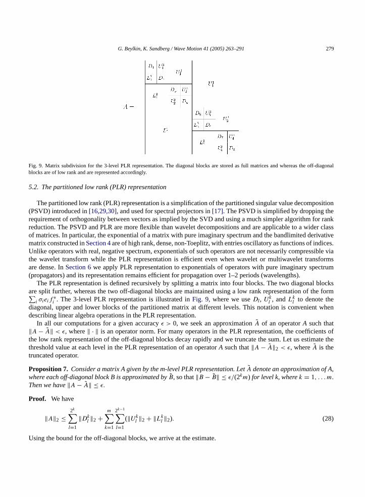
Fig. 9. Matrix subdivision for the 3-level PLR representation. The diagonal blocks are stored as full matrices and whereas the off-diagonalblocks are of low rank and are represented accordingly.

5.2. The partitioned low rank (PLR) representation

The partitioned low rank (PLR) representation is a simplification of the partitioned singular value decomposition(PSVD) introduced in[16,29,30], and used for spectral projectors in[17]. The PSVD is simplified by dropping therequirement of orthogonality between vectors as implied by the SVD and using a much simpler algorithm for rankreduction. The PSVD and PLR are more flexible than wavelet decompositions and are applicable to a wider classof matrices. In particular, the exponential of a matrix with pure imaginary spectrum and the bandlimited derivativematrix constructed inSection 4are of high rank, dense, non-Toeplitz, with entries oscillatory as functions of indices.Unlike operators with real, negative spectrum, exponentials of such operators are not necessarily compressible viathe wavelet transform while the PLR representation is efficient even when wavelet or multiwavelet transformsare dense. InSection 6we apply PLR representation to exponentials of operators with pure imaginary spectrum(propagators) and its representation remains efficient for propagation over 1–2 periods (wavelengths).

The PLR representation is defined recursively by splitting a matrix into four blocks. The two diagonal blocksare split further, whereas the two off-diagonal blocks are maintained using a low rank representation of the form∑

i σieif∗i . The 3-level PLR representation is illustrated inFig. 9, where we useDl, Uk

l , andLkl to denote the

diagonal, upper and lower blocks of the partitioned matrix at different levels. This notation is convenient whendescribing linear algebra operations in the PLR representation.

In all our computations for a given accuracyε > 0, we seek an approximationA of an operatorA such that‖A − A‖ < ε, where‖ · ‖ is an operator norm. For many operators in the PLR representation, the coefficients ofthe low rank representation of the off-diagonal blocks decay rapidly and we truncate the sum. Let us estimate thethreshold value at each level in the PLR representation of an operatorA such that‖A − A‖2 < ε, whereA is thetruncated operator.

Proposition 7. Consider a matrix A given by the m-level PLR representation. LetA denote an approximation of A,where each off-diagonal block B is approximated byB, so that‖B − B‖ ≤ ε/(2km) for level k,wherek = 1, . . . m.Then we have‖A − A‖ ≤ ε.

Proof. We have

‖A‖2 ≤2k∑l=1

‖Dkl ‖2 +

m∑k=1

2k−1∑l=1

(‖Ukl ‖2 + ‖Lk

l ‖2). (28)

Using the bound for the off-diagonal blocks, we arrive at the estimate.


Let a matrixAbe in anm-level PLR representation. In order to compute the matrix–vector productAu, it is clearfrom Fig. 9 that there are two types of matrix–vector multiplications we need to evaluate. We need to compute thedense matrix–vector products for the diagonal blocks and the matrix–vector productsLk

l u andUkl u, whereu ∈ C

Nk ,Nk = N/2k. If Lk

l = ∑ri=1 sieif

∗i , then the matrix–vector product is computed as

Lkl u =

r∑i=1

si〈u, fi〉ei. (29)

The cost of such matrix–vector multiplication is O(rNk). Assuming that the rank of all off-diagonal blocks is thesame, the total cost of computingAu is then estimated as 2mN2

m +∑mk=1 2krNk. If the total size ofA is N = 2m,

then we have the estimate of the total cost of matrix–vector multiplication in the PLR representation as O(N + rN

logN).We next describe an algorithm for computing the product of two matrices given in the PLR representation.

Consider the matrix productAB, whereA andB are matrices in them-level PLR representation. We considerA andB as the block matrices,

A =[A11 A12

A21 A22

]and B =

[B11 B12

B21 B22

],

where off-diagonal blocks are of the form∑r

i=1 σieif∗i and the diagonal blocks are in them − 1-level PLR

representation. The product ofA and B involves three types of block multiplications. The first is the prod-uct between two low rank representations, and such multiplication preserves the low rank form. The secondis the product between them − 1-level PLR and a low rank representation which amounts to matrix–vectormultiplications described above. The resulting low rank representation has to be added at the appropriate lev-els of the PLR representation and the rank of the result reduced via an algorithm described below. The thirdtype of block multiplication is the product between the twom − 1-level PLR representations which we treatrecursively.

5.3. Rank reduction

In order to reduce the rank of a separated representation of the form∑r

i=1 σieif∗i , where‖ei‖ = ‖fi‖ = 1, we

need to orthogonalize either the vectors{ei}ri=1 or {fi}ri=1 to reveal the actual rank of the representation. We callsuch procedure an orthogonalization sweep and use the size of the dynamically adjustedσi as pivots in choosing theorder in which orthogonalization is performed. As we orthogonalize the vectors{ei}ri=1, we simultaneously modifythe vectors{fi}ri=1 as to maintain the representation.

Once the vectors{ei}ki=1 have been orthogonalized, we project the vectors{ei}ri=k+1 onto the orthogonal comple-

ment ofek, normalize, and modifyfk to maintain the representation. The vectors{ei}k+1i=1 are now an orthonormal

set and we continue the procedure recursively. We also use the dynamically computedσi to truncate this process asσi become smaller than the threshold of accuracy.

After one orthogonalization sweep, only one set of vectors remains orthogonal and we may choose to repeat theprocedure for the other set. Such iterations eventually converge to the SVD. Since we do not require orthogonalityin separated representations, we typically perform only two orthogonalization sweeps. This algorithm is brieflydescribed in[15], where a significantly more complicated algorithm for reducing the separation rank is presentedfor higher dimensions.


6. Solution of the acoustic equation in two dimensions

Let us consider the acoustic equation

utt = 1

κ[(σux)x + (σuy)y] + F (30)

with the initial conditionsu(x, y, t)|t=0 = f (x, y), ut(x, y, t)|t=0 = g(x, y) and the boundary conditionu|∂D = h,where (x, y) ∈ D andt ∈ [0,∞). Here the functionκ = κ(x, y) is the compressibility, and the functionσ = σ(x, y)is the specific volume (the inverse of density) of the medium.

We consider the domainD to be a rectangle which is subdivided, if necessary, into rectangular subdomains. Weare using bandlimited functions on intervals and, thus, can subdivide without inflicting an unreasonable increase inthe number of terms in the representation of functions on subdomains. In the future extensions of our approach formore general domainsD, we plan to subdivide them into subdomains and map such subdomains into rectangles sothat we can use the tools developed in this paper.

Let us first rewrite the acoustic equation(30) as a first order system in time. Since the coefficientsκ andσ aretime independent, the propagator for the homogeneous problem (F = 0) is given by the exponential of a matrix.We represent the spatial operator by the separated representation described inSection 5.1which decomposes theoperator into a short sum of matrices acting in one dimension. We then compress these matrices using the PLRrepresentation inSection 5.2.

Following the derivation by Bazer and Burridge[14], we introduce the functionsv andw, and write the acousticequation(30)as

w

v

u

t

=

0 0 σ∂b

∂x

0 0 σ∂b

∂y

1

κ

∂

∂x

1

κ

∂

∂y0

w

v

u

+

0

0∫ t

0 F (x, y, τ) dτ

, (31)

where each block is given in its separated representation. Here∂b/∂x and∂b/∂y denote differentiation operatorswith boundary conditions imposed in thex andy direction. We rewrite equation(31)as

ut = Lu+ F, with u(0) = u0, (32)

whereu = [ w v u ]T andL is the linear operator incorporating the block matrix on the right-hand side of(31). Usingbases for bandlimited functions (or finite differences in comparison codes), we discretize(32) in space resulting ina finite-dimensional system of ODEs. IfL is time independent, thenu(t) = etL u0.

Eq. (32)is then solved by

u(t) = P(t)u0 + P(t)∫ t

0P(τ)−1F(τ) dτ,

where the propagatorP(t) is an operator solving the integral equation:

P(t) = I +∫ t

0L(τ)P(τ) dτ.

We constructL using derivative operators for bandlimited functions with boundary and interface conditions incor-porated according toSection 3and propagate the solution by applying the matrix exponential etL . Let us describe


a numerical scheme for solving the homogeneous acoustic Eq.(30) in two dimensions with time independentcoefficients and boundary conditions. We proceed via the following steps:

(1) Construct the derivative matrices representing∂/∂x, ∂b/∂x, ∂/∂y and∂b/∂y using the results inSection 3.(2) Construct separated representations of the multiplication operators 1/κ(x, y) andσ(x, y)(3) Construct blocks of the 3× 3 spatial operator in(31)and use the algorithm inSection 5.3to reduce the separation

rank of each block.(4) Select the time stept (see below) and compute the matrix exponential etL using the scaling and squaring

algorithm (see e.g.[31]). The linear combinations and products of the matrix blocks given in the separatedrepresentation are computed using the methods described inSection 5.

(5) Compute the solutionu(tk) = etL u(tk−1), starting fromu(t0) = u(0), for k = 1, . . . , Ntime.

We refer to this algorithm as the method of bandlimited bases (MBB) with the exponential propagator (EP). Wenote that for time dependent boundary conditions the problem can be reduced to that with zero boundary conditionsand a forcing term.

If the factors in the separated representation (which are ordinary matrices) are large, we use the PLR representationdescribed inSection 5.2to speed up the computations in Steps 4 and 5 above. As discussed inSection 4, the normof the derivative projectors can be greatly reduced by using spectral projectors. For example, to construct projectedversions of∂/∂x and∂b/∂x (derivative operators in thex-direction), we form the block matrix,

L =[

0 D0

D 0

],

whereD andD0 are constructed as inSection 3. The boundary conditions are enforced only for the functionu in(31)which results in the structure of the matrixL above. We then construct the projected operator,

Lproj =∑

|λk |≤c

λkekf Tk ,

whereek andfk are the left and the right eigenvector ofL, scaled so thatf Tk ek = 1. The projected version of∂/∂xis now given by the lower left block ofLproj, and the projected version of∂b/∂x for zero boundary conditions isgiven by the upper right block ofLproj. Using these blocks, we assemble the 3× 3 block-matrix representation ofthe operator in(31).

In most numerical methods for wave propagation, the time step is restricted by the Courant–Friedrich–Lewy(CFL) condition (see e.g.[32]). According to the CFL condition, the spatial step is controlled by the speed ofthe propagating waves to ensure stability. When using the matrix exponential, the time stept can be chosen aslarge as desired without causing instabilities as long as the operatorL has no eigenvalues with positive real part.In our approach a very large time step will increase the separation rank and the ranks in the partitioned low rankrepresentation. We have found that choosing the time step between 0.5 and 2 periods gives a good compromisebetween an efficient representation of the matrix exponential and the number of time steps.

In solving the equation, we maintain solutions at the quadrature nodes of the bandlimited representation. Forillustrations, we interpolate the result to an equally spaced grid (seeSection 14).

6.1. Comparison of the results

We compare the MBB with the exponential propagator (MBB with EP) to two other methods. In the firstcomparison we use the MBB but replace Steps 4 and 5 with the explicit RK4 solver in time (MBB with RK4). In


the second comparison we write the acoustic equation (30) as a first order system:

[v

u

]t

=

0

1

κ

[∂

∂x

(σ∂b

∂x

)+ ∂

∂y

(σ∂b

∂y

)]

I 0

[v

u

]+[F

0

](33)

and discretize it in space using the fourth-order finite difference stencil on an equally spaced grid including theendpoints (see[25]) and use the explicit RK4 solver in time (FD with RK4).

To compare methods for solving the acoustic equation, we introduce the characteristic time and length scales.Let us consider on [−1,1] the wave equationutt = uxx with the zero boundary conditions. This equation describesa medium with the unit compressibility and specific volume and, thus, the unit velocity. For the initial conditionsu(x,0) = sin((kπ/2)(x + 1)) andut(x,0) = 0, and each integerk, we have the solution

u(x, t) = sin(12(kπ)(x + 1)) cos(12(kπ)t).

Since the velocity is equal to 1, we define the characteristic period,τ = π/b, and the characteristic length scale,λ = π/b, whereb = kπ/2 is the bandlimit. For periodic solutions in dimensiond = 1, the Nyquist sampling rate(in time) requires two samples per characteristic periodτ. We note that in dimensiond = 2, for sampling purposesthe corresponding time period has an extra factor

√2 since the solutions ofutt = uxx + uyy in [−1,1] × [−1,1],

with the zero boundary condition and the initial conditionsu(x, y,0) = sin((kπ/2)(x + 1)) sin((kπ/2)(y + 1)) andut(x, y,0) = 0, contain the factor cos(

√2πt/τ).

6.1.1. Comparison of accuracy and speed for constant coefficientsFor our first set of experiments, we solve

utt = uxx + uyy, (x, y) ∈ (−1,1) × (−1,1),

u(x, y,0) = sin(12(π(x + 1))) sin(12(π(y + 1))) + sin(b(x + 1)) sin(b(y + 1)),

u(±1, y) = u(x,±1) = ut(x, y,0) = 0, (34)

whereb = kπ/2 for some integerk > 1, and the solution is given by

u(x, y, t) = sin

(π(x + 1)

2

)sin

(π(y + 1)

2

)cos

(π√2t

)+ sin(b(x + 1)) sin(b(y + 1)) cos(

√2bt).

We note that this solution contains both low frequency (the first term) and high frequency (the second term) modes.For the experiments in this section, we measure the error of the vectoru = [ w v u ]T using the relative norm,namely, ifu approximates the exact solutionu, then

error= ‖u− u‖∞‖u‖∞

.

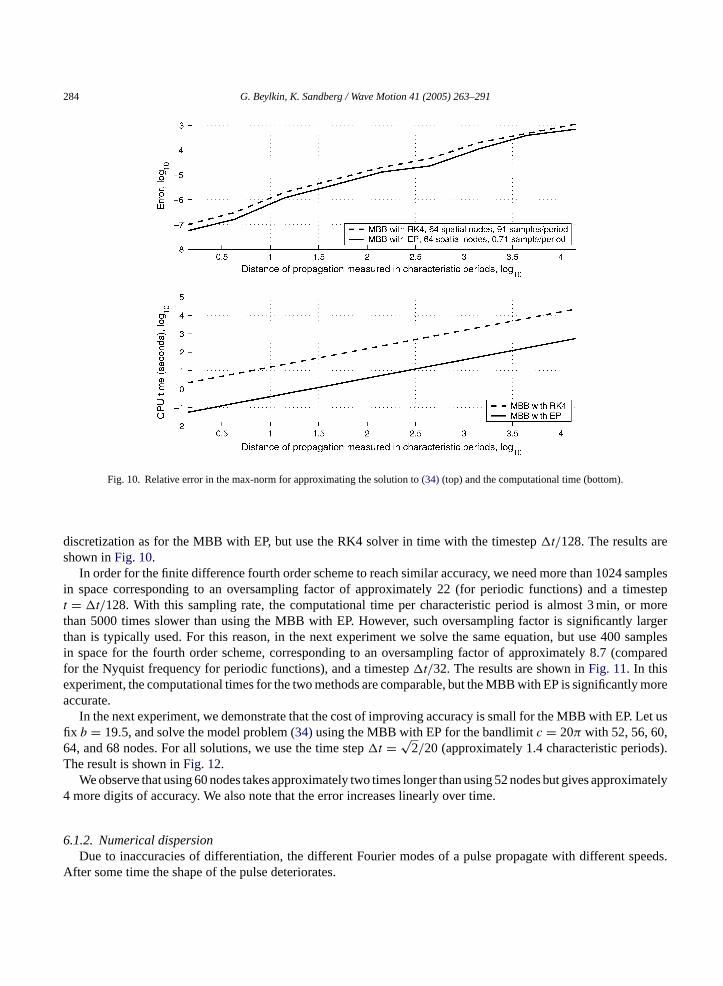
In the first experiment, we solve(34) usingb = 22.5π. We propagate the solution and evaluate the error over arange of approximately 1–104 characteristic periods, and also record the CPU time it took to produce the solution.

For the MBB with EP, we construct 64 quadrature nodes and weights for the bandlimitc = 23π, which for periodicfunctions corresponds to an oversampling factor of approximately 1.4. We set the accuracy in the constructionto ε = 10−7 resulting in 64 nodes, and select the time stept = √

2/23 corresponding to approximately 1.4characteristic periods. We represent the operator using the separated and PLR representations. This results inthe separation rankr = 5 for the blocks in the exponential operator. For comparison, we use the same spatial


Fig. 10. Relative error in the max-norm for approximating the solution to(34) (top) and the computational time (bottom).

discretization as for the MBB with EP, but use the RK4 solver in time with the timestept/128. The results areshown inFig. 10.

In order for the finite difference fourth order scheme to reach similar accuracy, we need more than 1024 samplesin space corresponding to an oversampling factor of approximately 22 (for periodic functions) and a timestept = t/128. With this sampling rate, the computational time per characteristic period is almost 3 min, or morethan 5000 times slower than using the MBB with EP. However, such oversampling factor is significantly largerthan is typically used. For this reason, in the next experiment we solve the same equation, but use 400 samplesin space for the fourth order scheme, corresponding to an oversampling factor of approximately 8.7 (comparedfor the Nyquist frequency for periodic functions), and a timestept/32. The results are shown inFig. 11. In thisexperiment, the computational times for the two methods are comparable, but the MBB with EP is significantly moreaccurate.

In the next experiment, we demonstrate that the cost of improving accuracy is small for the MBB with EP. Let usfix b = 19.5, and solve the model problem(34)using the MBB with EP for the bandlimitc = 20π with 52, 56, 60,64, and 68 nodes. For all solutions, we use the time stept = √

2/20 (approximately 1.4 characteristic periods).The result is shown inFig. 12.

We observe that using 60 nodes takes approximately two times longer than using 52 nodes but gives approximately4 more digits of accuracy. We also note that the error increases linearly over time.

6.1.2. Numerical dispersionDue to inaccuracies of differentiation, the different Fourier modes of a pulse propagate with different speeds.

After some time the shape of the pulse deteriorates.


Fig. 11. Relative error (log10) in the max-norm for approximating the solution to(34) (top), and the computational time (bottom).

Fig. 12. Relative error in the max-norm for approximating the solution to(34) for b = 19.5π using two different sampling rates (top). The CPUtime for propagating the wave one characteristic period for a varying number of nodes (bottom).


To examine this phenomenon, let us consider the wave equation in one dimension,ut + cux = 0, the solutionsof which correspond to right-traveling waves. Solutions of this equation take the form:

u(x, t) = eiω(x−ct),

which we refer to as a Fourier mode of frequencyω traveling to the right with velocityc. Exact differentiation ofthis solution yields

∂

∂xu = iω eiω(x−ct).

If the error in the representation of the differentiation operator is of the form

∂

∂xu � i f(ω) eiω(x−ct),

then the Fourier mode propagates with the velocitycf (ω)/ω. Unlessf (ω) = ω, which corresponds to the exactdifferentiation, the Fourier modes of different frequencies travel with different velocities. For example, in the caseof the second order centered finite difference approximation of the derivative,f (ω) = sin(ω).

Fig. 13. Solution of(35)using the MBB with EP. The shape of the pulse is maintained throughout the propagation.


In this section we compare numerical dispersion using the MBB with EP and the FD with RK4 described inSection 6.1. Let us solve

utt = uxx + uyy, (x, y) ∈ (−2,2) × (−2,2), u(x, y,0) = sinc2(27πx)sinc2(27πy),

u(±2, y) = u(x,±2) = ut(x, y,0) = 0. (35)

The solution is a sharp pulse originating at the center of the domain, and expanding outward. In the absence ofnumerical dispersion, the shape of the pulse should be maintained.

For the MBB with EP, we construct 128 quadrature nodes and weights for the bandlimitc = 54π. We set theaccuracy in the construction toε = 10−7. We divide the domain into four subdomains and approximate the solutionon each subdomain using 128-by-128 nodes. We use the time stept = 2π/c corresponding to propagating twocharacteristic wavelengths, and represent the operator using the separated and PLR representations. This resultsin separation rank eitherr = 5 or 6 for the blocks of the exponential operator. For the fourth order scheme, weuse 432 samples in space and the timestept = π/10c corresponding to propagating a tenth of the characteristicwavelength. This sampling rate yields approximately the same computational time for the two schemes. The resultsare shown as sequences of images inFigs. 13 and 14.

We note that in the MBB with EP the shape of the pulse is maintained. For the FD with RK4, the pulse begins tonoticeably deteriorate, as the error accumulates due to the numerical dispersion. The numerical dispersion affectsour method as well but at a much slower rate.

Fig. 14. Solution of(35)using the FD with RK4. Note the ripples near the wave front which are caused by numerical dispersion.


6.1.3. Numerical results for variable coefficientsLet us consider the acoustic equation with variable coefficients. Since we do not have an analytical solution, we

simply display a sequence of images and study the shape of the pulse as it propagates throughout the domain. Letus solve

utt = 1

κ(y)(uxx + uyy), (x, y) ∈ (−1,1) × (−1,1), u(x, y,0) = e−1000(x2+y2),

u(±1, y) = u(x,±1) = ut(x, y,0) = 0, (36)

where

κ(y) = 1

1 − sin(π(y + 1))/2.

The solution is a sharp pulse originating at the origin of the domain, and expanding outwards in the medium withvarying velocity. For the MBB with EP, we construct 128 quadrature nodes and weights for the bandlimitc = 54π.We set the accuracy in the construction toε = 10−7. We use the time stept = 2π/c corresponding to propagatingover two characteristic wavelengths. This choice of parameters yields the separation rank eitherr = 7 or 8 for theblocks of the exponential operator. Using the PLR representation for computing etL u is in this case approximately25% faster than using the dense representation of matrices in one dimension. The gain due to PLR increases forlarger problems. For the FD with RK4, we use 216 samples in space and the timestept = π/10c, corresponding

Fig. 15. Solution of(35)using the MBB with EP.


Fig. 16. Solution of(35)using the FD with RK4. Note the ripples which are caused by numerical dispersion.

to propagating over one-tenth of the characteristic wavelength. This sampling rate gives the two schemesapproximately the same computational time. The results are shown as sequences of images inFigs. 15 and 16.

Both solutions behave qualitatively in the same way by propagating faster in the upper part of the domain wherethe wave velocity is higher. We note that for the MBB with EP, the shape of the pulse is maintained. For the FDwith RK4, the pulse begins to noticeably deteriorate, as the error accumulates due to the numerical dispersion.

Appendix A. Proof of Theorem 3

First, let us consider a functionv ∈ Bc ∩ L1(R). Using the Fourier transform, we write it (almost everywhere) as

v(x) =∫ c

−c

σ(ω) eiωx dω,

whereσ is continuous and bounded sincev ∈ L1(R). Let us definebk = −c + (2kc/N) for k = 1, . . . , N. Then|bk| ≤ c and we can approximatev with the Riemann sum,

v(x) = 2c

N

N∑k=1

σ(bk) eibkx + EN(x),


where limN→∞ EN (x) = 0 for all x ∈ [−1,1]. We chooseN sufficiently large, such that‖EN‖L∞[−1,1] < ε/2√

2and define forx ∈ [−1,1]

u(x) =N∑

k=1

ak eibkx,

whereak = 2cσ(bk)/N. Thenu is bounded on [−1,1] and|v(x) − u(x)| < ε/2√

2 almost everywhere.Next we consider a functionu ∈ Bc. Then, sinceBc ∩ L1(R) is dense inBc, there exists a functionv ∈ Bc ∩ L1(R)

such that

‖u − v‖L2[−1,1] <ε2. (A.1)

As we showed above, there exists ˜u ∈ Ec such that|v(x) − u(x)| < ε/2√

2 almost everywhere on [−1,1] and, hence,

‖v − u‖2L2[−1,1] =

∫ 1

−1|v(x) − u(x)|2 dx ≤ ε2

4,

which combined with(A.1) gives us

‖u − u‖L2[−1,1] ≤ ‖u − v‖L2[−1,1] + ‖v − u‖L2[−1,1] < ε.

Acknowledegement

This research was supported in part by NSF/ITR grant DMS-0219326 (GB and KS), DOE grant DE-FG02-03ER25583 and NIMA grant NMA401-02-1-2002 (GB).

References

[1] D. Slepian, H.O. Pollak, Prolate spheroidal wave functions, Fourier analysis and uncertainty I, Bell Syst. Technol. J. 40 (1961) 43–63.[2] H.J. Landau, H.O. Pollak, Prolate spheroidal wave functions, Fourier analysis and uncertainty II, Bell Syst. Technol. J. 40 (1961) 65–84.[3] H.J. Landau, H.O. Pollak, Prolate spheroidal wave functions, Fourier analysis and uncertainty III, Bell Syst. Technol. J. 41 (1962) 1295–

1336.[4] D. Slepian, Prolate spheroidal wave functions, Fourier analysis and uncertainty IV. Extensions to many dimensions, generalized prolate

spheroidal functions, Bell Syst. Technol. J. 43 (1964) 3009–3057.[5] D. Slepian, Prolate spheroidal wave functions, Fourier analysis and uncertainty V. The discrete case, Bell Syst. Technol. J. 57 (1978)

1371–1430.[6] H. Xiao, V. Rokhlin, N. Yarvin, Prolate spheroidal wavefunctions, quadrature and interpolation, Inverse Probl. 17 (4) (2001) 805–838.[7] G. Beylkin, L. Monzon, On generalized Gaussian quadratures for exponentials and their applications, Appl. Comput. Harmon. Anal. 12

(3) (2002) 332–373.[8] D. Gottlieb, S.A. Orszag, Numerical analysis of spectral methods: theory and applications, in: CBMS-NSF Regional Conference Series in

Applied Mathematics, No. 26, Society for Industrial and Applied Mathematics, Philadelphia, PA, 1977.[9] J.P. Boyd, Prolate spheroidal wave functions as an alternative to Chebyshev and Legendre polynomials for spectral element and psedospectral

algorithms, Preprint.[10] Q. Chen, D. Gottlieb, J. Hesthaven, Spectral methods based on prolate spheroidal wave functions for hyperbolic PDEs, Preprint.[11] B. Alpert, G. Beylkin, D. Gines, L. Vozovoi, Adaptive solution of partial differential equations in multiwavelet bases, J. Comput. Phys.

182 (1) (2002) 149–190.[12] B. Alpert, L. Greengard, T. Hagstrom, An integral evolution formula for the wave equation, J. Comput. Phys. 162 (2000) 536–543.[13] H. Tal-Ezer, Spectral methods in time for hyperbolic equations, SIAM J. Numer. Anal. 23 (1) (1986) 11–26.


[14] J. Bazer, R. Burridge, Energy partition in the reflection and refraction of plane waves, SIAM J. Appl. Math. 34 (1978) 78–92.[15] G. Beylkin, M.J. Mohlenkamp, Numerical operator calculus in higher dimensions, Proc. Natl. Acad. Sci. USA 99 (16) (2002) 10246–10251.[16] P. Jones, J. Ma, V. Rokhlin, A fast direct algorithm for the solution of the Laplace equation on regions with fractal boundaries, J. Comput.

Phys. 113 (1) (1994).[17] G. Beylkin, N. Coult, M.J. Mohlenkamp, Fast spectral projection algorithms for density-matrix computations, J. Comput. Phys. 152 (1)

(1999) 32–54.[18] G. Beylkin, M.J. Mohlenkamp, Algorithms for numerical analysis in high dimensions, University of Colorado, Applied Mathematics

Preprint # 519, 2004, SIAM J. Sci. Comp. (2004), in press.[19] H. Tal-Ezer, R. Kosloff, An accurate and efficient scheme for propagating the time dependent Schrodinger equation, The J. Chem. Phys.

81 (9) (1984) 3967–3971.[20] D. Slepian, Some comments on Fourier analysis, uncertainty and modeling, SIAM Rev. 25 (3) (1983) 379–393.[21] Y. Meyer, Wavelets and operators, Cambridge Studies in Advanced Mathematics, vol. 37, Cambridge University Press, Cambridge, 1992

(transl.; from the 1990 French original by D.H. Salinger).[22] T. Rivlin, Chebyshev Polynomials, 2nd ed., Wiley, 1990.[23] D. Kosloff, H. Tal-Ezer, A modified Chebyshev pseudospectral method with an O(N−1) time step restriction, J. Comput. Phys. 104 (2)

(1993) 457–469.[24] J.S. Hesthaven, P.G. Dinesen, J.P. Lynov, Spectral collocation time-domain modeling of diffractive optical elements, J. Comput. Phys. 155

(2) (1999) 287–306.[25] B. Fornberg, A Practical Guide to Pseudospectral Methods, Cambridge University Press, 1995.[26] J.P. Boyd, Chebyshev and Fourier Spectral Methods, 2nd ed., Dover, Mineola, NY, 2001.[27] L. Greengard, Spectral integration and two-point boundary value problems, SINUM 28 (4) (1991) 1071–1080.[28] J.A.C. Weideman, L.N. Trefethen, The eigenvalues of second-order spectral differentiation matrices, SIAM J. Numer. Anal. 25 (6) (1988)

1279–1298.[29] T. Hrycak, V. Rokhlin, An improved fast multipole algorithm for potential fields, SIAM J. Sci. Comp. 19 (6) (1998) 1804–1826.[30] N. Yarvin, V. Rokhlin, A generalized one-dimensional fast multipole method with application to filtering of spherical harmonics, J. Comput.

Phys. 147 (2) (1998) 594–609.[31] G. Golub, C.V. Loan, Matrix Computations, 3rd ed., Johns Hopkins University Press, 1996.[32] A. Iserles, A First Course in the Numerical Analysis of Differential Equations, Cambridge University Press, 1996.

Wave propagation using bases for bandlimited functions

Documents

Transcript of Wave propagation using bases for bandlimited functions