Wave propagation in a non-uniform, magnetised plasma:

Finite beta

James McLaughlin

Leiden

March 2005

Introduction

• Models of wave motions that should occur in the neighbourhood of 2D X-point. There are three types of wave motions that should occur; slow MA, fast MA and Alfvén. Wave motions recently observed in the corona.

• Research has also illustrated importance of magnetic topology. Extrapolations predict null points; Alfvén speed zero.

• Aim - Bring these areas together. Show how plasma waves behave when they travel into magnetic structures (inhomogeneous medium).

Model

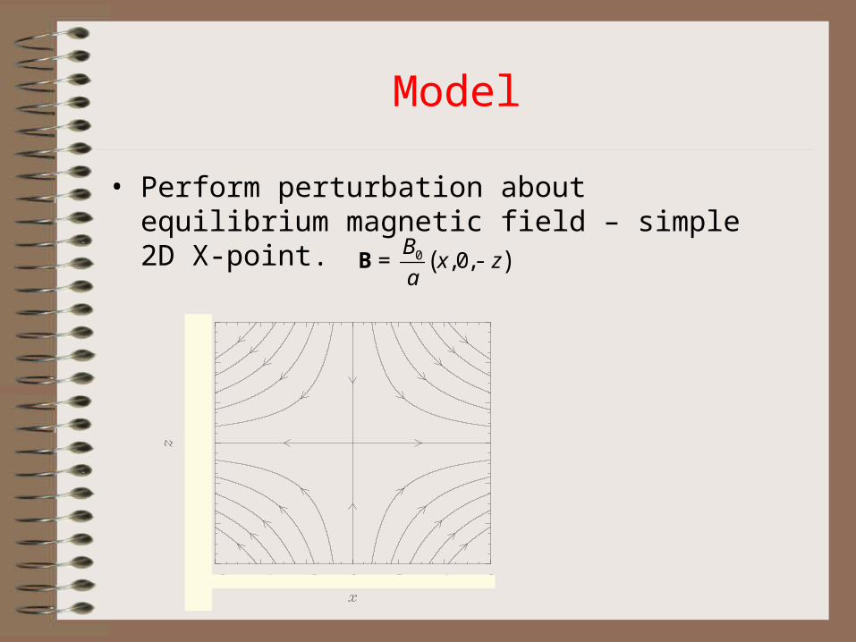
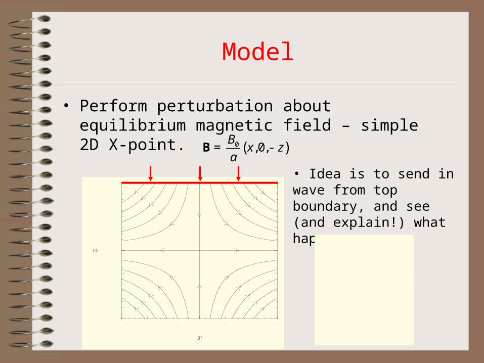
• Perform perturbation about equilibrium magnetic field – simple 2D X-point.

( )0 ,0,B

x za

= -B

Model

• Perform perturbation about equilibrium magnetic field – simple 2D X-point.

( )0 ,0,B

x za

= -B

• Idea is to send in wave from top boundary, and see (and explain!) what happens.

Model II

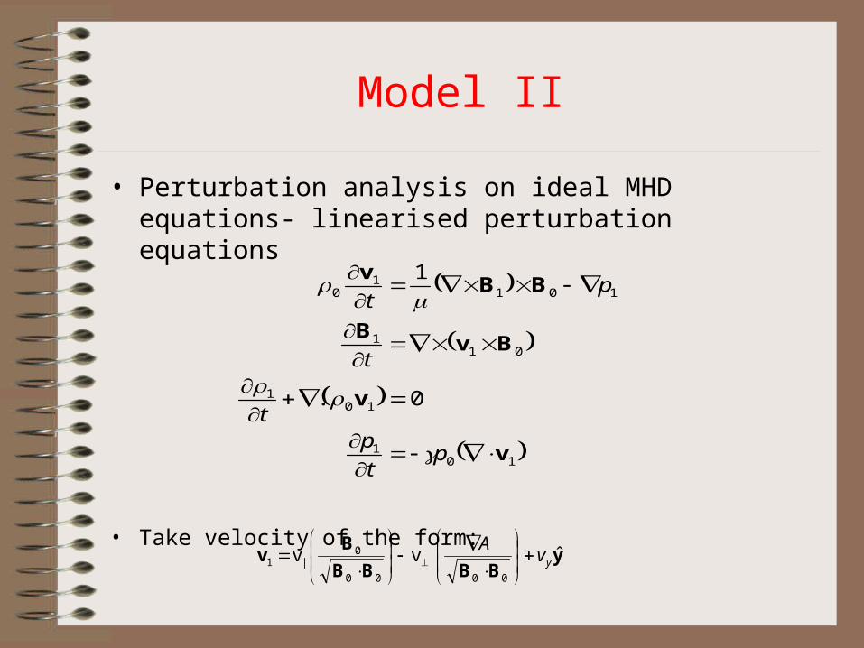
• Perturbation analysis on ideal MHD equations- linearised perturbation equations

• Take velocity of the form:

101

101

011

1011

0

0.

1

v

v

BvB

BBv

pt

pt

t

pt

yBBBB

Bv ˆvv

0000

0||1 yv

A

Model III

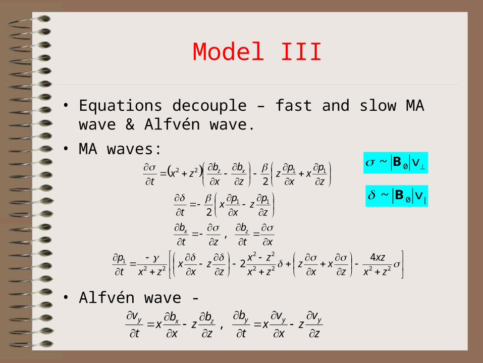
• Equations decouple – fast and slow MA wave & Alfvén wave.

• MA waves:

• Alfvén wave -

2222

22

221

11

1122

42

,

2

2

zx

xz

zx

xz

zx

zx

zz

xx

zxt

p

xt

b

zt

b

z

pz

x

px

t

z

px

x

pz

z

b

x

bzx

t

zx

xz

z

vz

x

vx

t

b

z

bz

x

bx

t

v yyyzxy

,

v~ 0B

||0 v~ B

Fast MA wave I

• Fast wave case reduces to single wave equation:

• Where (non-dimensionalised. Spatially dependent).

• Fast wave solved numerically - two-step Lax-Wendroff scheme. -6 ≤ x ≤ 6 and -6 ≤ z ≤ 6 .

• Boundary conditions

2 2Av x z= +

2

2

2

22

2

2

,zx

zxvt A

0

0,0,0

otherwise0

0sin6,

666

zxx zxx

ttx

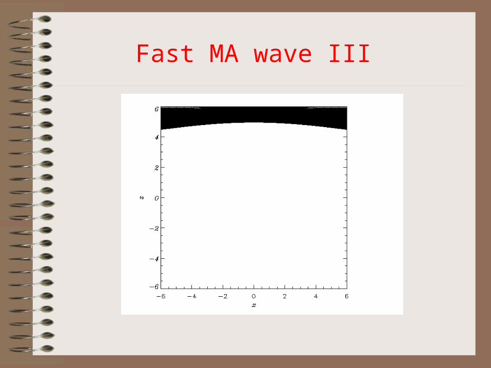
Fast MA wave III

Fast MA wave II

• Linear, fast magnetoacoustic wave travels towards the vicinity of the X-point and bends around it.

• Alfvén speed spatially varying - travels faster further away from the origin.

• Wave demonstrates refraction – wraps wave around null

• Key feature of fast wave propagation.

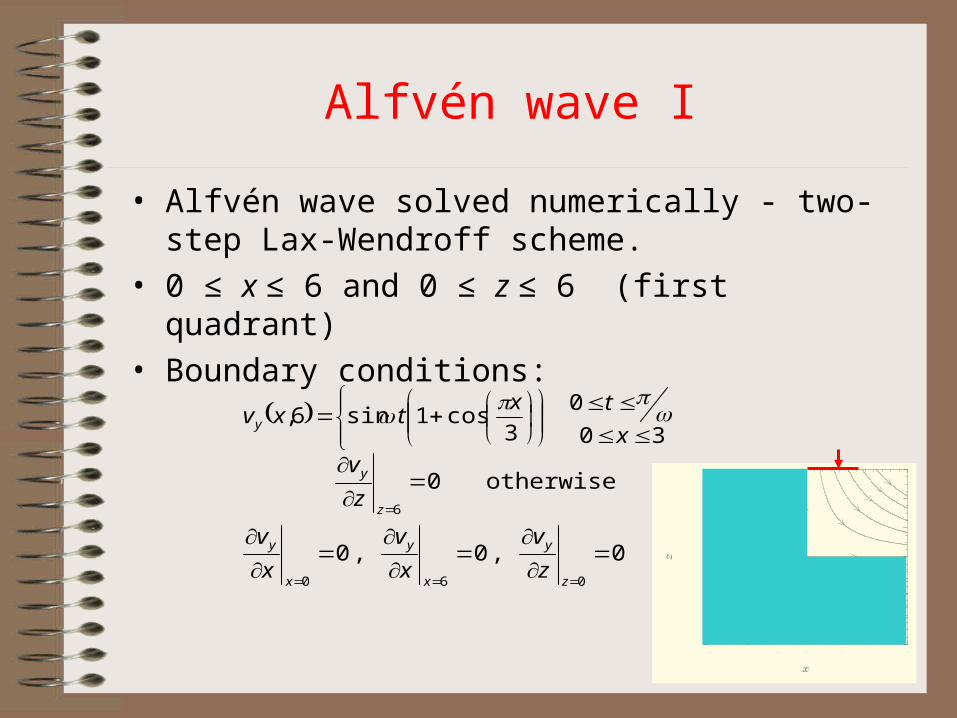
Alfvén wave I

• Alfvén wave solved numerically - two-step Lax-Wendroff scheme.

• 0 ≤ x ≤ 6 and 0 ≤ z ≤ 6 (first quadrant)

• Boundary conditions:

0,0,0

otherwise0

30

03

cos1sin6,

060

6

z

y

x

y

x

y

z

y

y

z

v

x

v

x

v

z

vx

txtxv

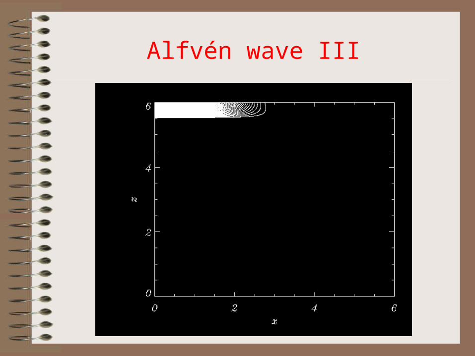
Alfvén wave III

Alfvén wave II

• Alfvén wave travels down from top boundary and begins to spread out, following the field lines.

• As the wave approaches the separatrix, thins but keeps its original amplitude. The wave eventually accumulates very near the separatrix (x axis).

Fast and slow MA waves

• How does this simple model change with the inclusion of a finite term?

• Main questions:

1. How does the slow wave couple to the (driven) fast wave?

2. How does the nature of the coupling change with ?

3. What is the effect of pressure at the origin?

Fast and slow I

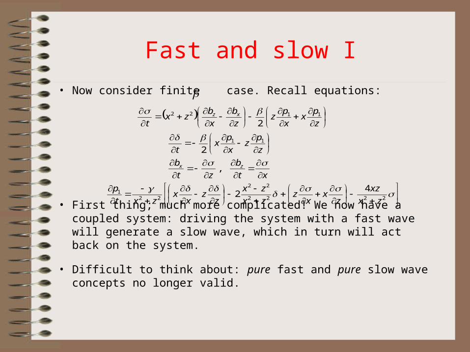
• Now consider finite case. Recall equations:

• First thing; much more complicated! We now have a coupled system: driving the system with a fast wave will generate a slow wave, which in turn will act back on the system.

• Difficult to think about: pure fast and pure slow wave concepts no longer valid.

2222

22

221

11

1122

42

,

2

2

zx

xz

zx

xz

zx

zx

zz

xx

zxt

p

xt

b

zt

b

z

pz

x

px

t

z

px

x

pz

z

b

x

bzx

t

zx

xz

Fast and slow II

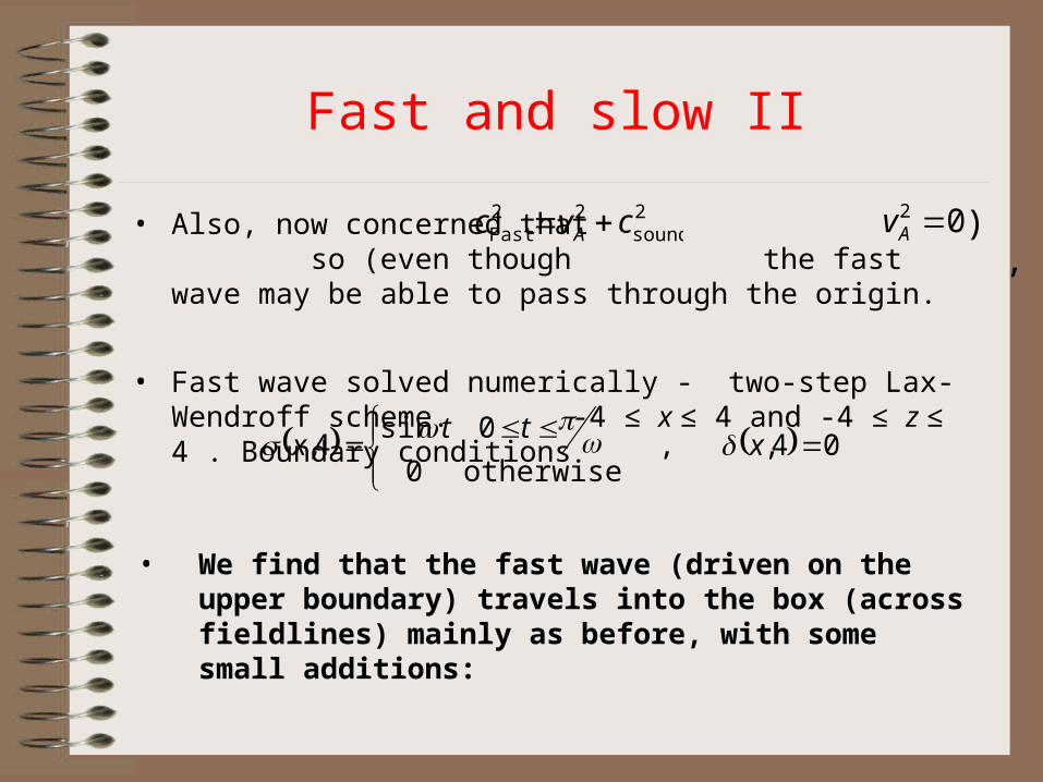
• Also, now concerned that so (even though the fast wave may be able to pass through the origin.

• Fast wave solved numerically - two-step Lax-Wendroff scheme.

-4 ≤ x ≤ 4 and -4 ≤ z ≤ 4 . Boundary conditions

04,,otherwise0

0sin4,

x

ttx

2sound

22Fast cvc A 02 Av

• We find that the fast wave (driven on the upper boundary) travels into the box (across fieldlines) mainly as before, with some small additions:

),

Movies I

Fast zero beta : perpendicular velocity

Movies II

2.0

Perpendicular velocity component

Movies III

Parallel velocity component

Fast and slow

• Main questions:

1. How does the slow wave couple to the (driven) fast wave?

2. How does the nature of the coupling change with ?

3. What is the effect of pressure at the origin?

How does the slow wave couple to the (driven) fast wave? I

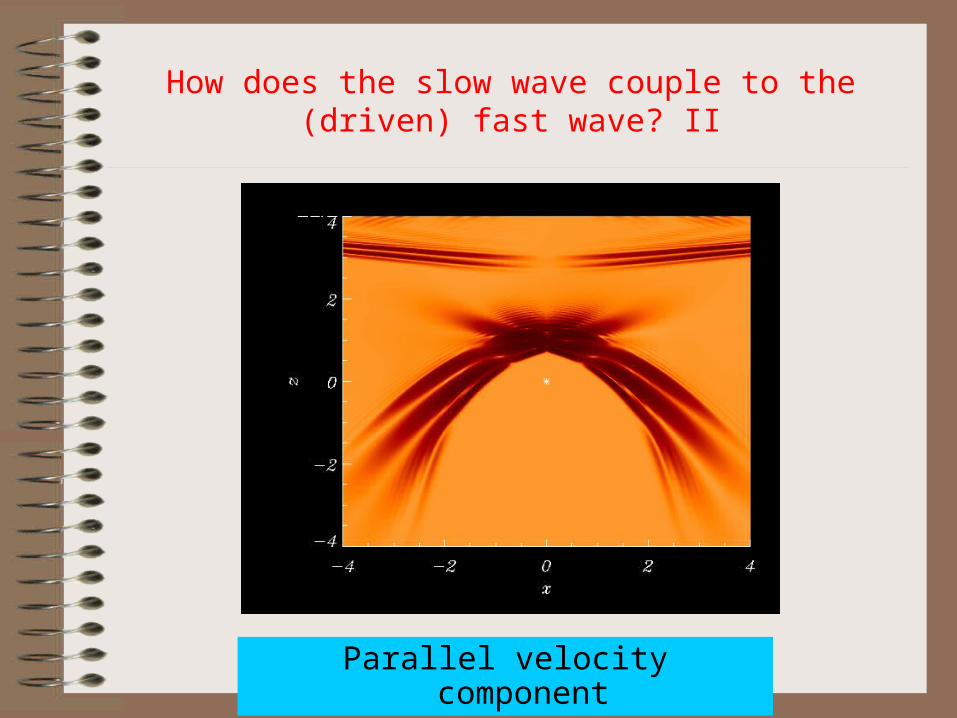
• There is now coupling to the parallel velocity component, such that two waves are produced:

firstly, an aspect travelling at the same speed and frequency as the driven (fast) wave; this wraps around the null in a similar way to the zero beta fast wave.

secondly, an aspect that trails behind the first, travelling at a much slower speed ( ). This is the slow wave.

How does the slow wave couple to the (driven) fast wave? II

Parallel velocity component

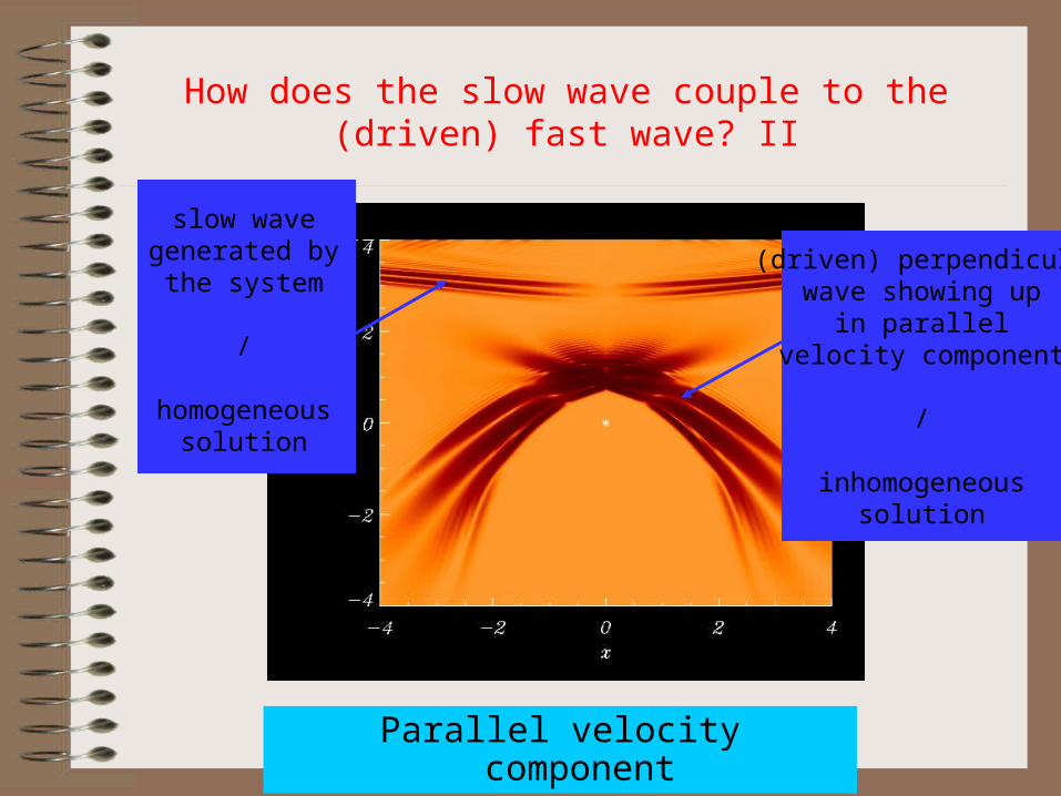
How does the slow wave couple to the (driven) fast wave? II

Parallel velocity component

How does the slow wave couple to the (driven) fast wave? II

slow wavegenerated bythe system

/

homogeneoussolution

(driven) perpendicularwave showing up

in parallelvelocity component

/

inhomogeneoussolution

Parallel velocity component

Fast and slow

• Main questions:

1. How does the slow wave couple to the (driven) fast wave?

2. How does the nature of the coupling change with ?

3. What is the effect of pressure at the origin?

How does the nature of the coupling change with ?

• The size of the used will affect the magnitude of the coupling and determine how much the pressure and parallel velocity feedback to affect the (driven) perpendicular velocity wave.

• In the corona, typical values of are often cited.01.0

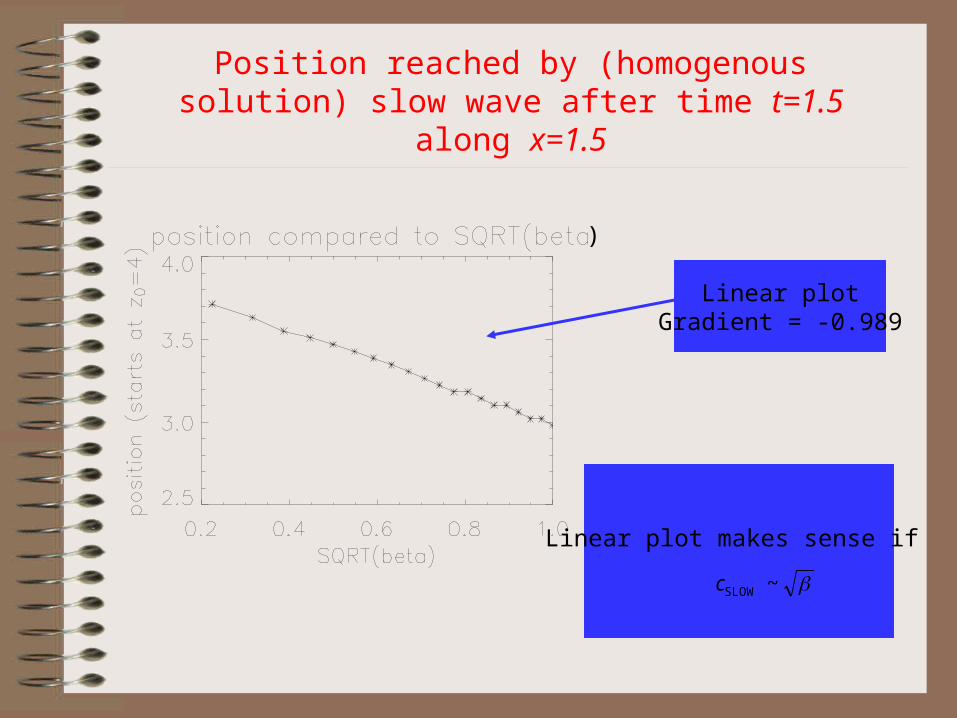
Position reached by (homogenous solution) slow wave after time t=1.5 along x=1.5

)

Linear plotGradient = -0.989

Linear plot makes sense if

~SLOWc

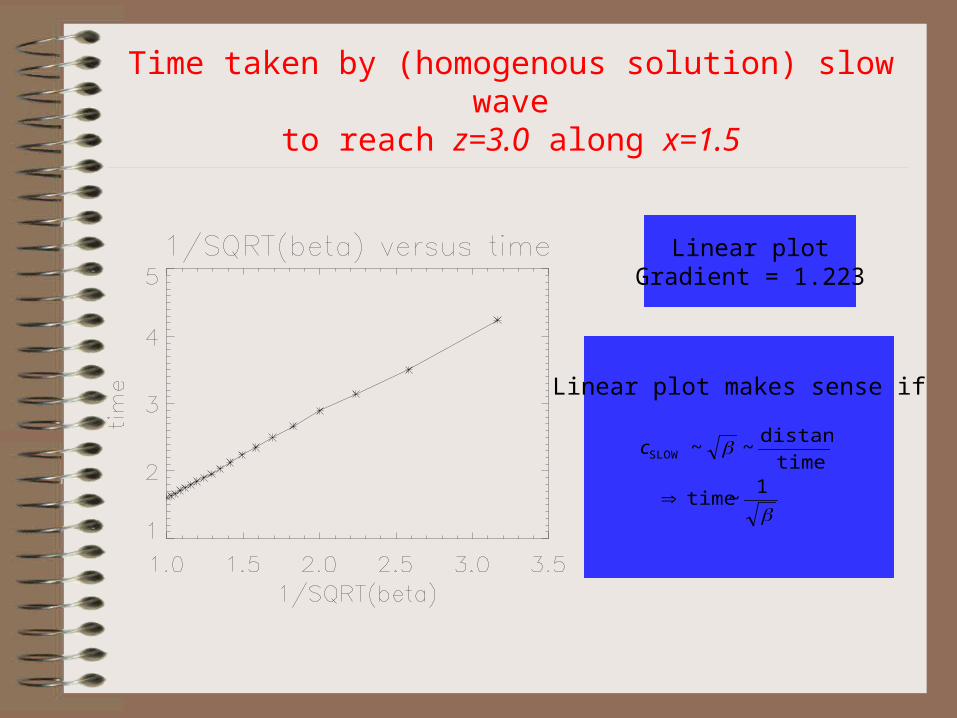
Time taken by (homogenous solution) slow waveto reach z=3.0 along x=1.5

Linear plotGradient = 1.223

Linear plot makes sense if

1~time

time

distance~~SLOW

c

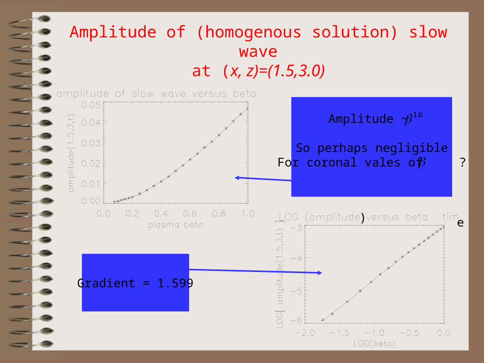
Amplitude of (homogenous solution) slow waveat (x, z)=(1.5,3.0)

) e

Gradient = 1.599

Amplitude ~

So perhaps negligibleFor coronal vales of ?

6.1

Amplitude of (inhomogenous solution) waveat (x, z) = (0.5,1.0) at t=1.67

1~time

time

distance~~

sc

Linear plotGradient = 0.8702

Amplitude increases

Also, position of max alwaysoccurs at same point in space,

i.e. position of couplingindependent of

~

Fast and slow III

• Main questions:

1. How does the slow wave couple to the (driven) fast wave?

2. How does the nature of the coupling change with ?

3. What is the effect of pressure at the origin?

What is the effect of pressure at the origin? I

• Idea is that, as opposed to case, when all wave is packed around null, pressure may now critically change the results; i.e. either expel the wave away from the null or in some other way impede its propagation (because of the term).

• However, we do not find that the inclusion of a pressure term significantly changes the system.

• Yes, the pressure is increasing as we approach the null ( at null), and yet fast wave still wraps around the null in a very similar way to before, and so wave will still dissipate close to the origin.

• We also find no evidence of the fast wave travelling through the null (perhaps is still true, but may be tiny (so dissipates).

1p

0

2sound

22Fast cvc A

soundc

Conclusions I – Fast wave

• When fast magnetoacoustic wave propagates near X-type neutral point, wave wraps itself around due to refraction (at least in 2D).

• Large current density accumulation at the null.

Build up exponential in time.

• Refraction of the wave focuses energy of the incident wave towards null point - wave continues to wrap itself around null point, again and again.

Conclusions II – Alfvén wave

• Alfvén wave - wave propagates along field lines, accumulating on separatrix (along separatrices due to symmetry). Wave thins and stretches.

• The current jx increases and accumulates along the separatrix, whilst jz decays away.

Conclusions III – wave coupling

• Perpendicular and parallel velocity components now (inevitably) coupled with inclusion of .

• Driven perpendicular (fast) wave generates waves in parallel velocity component (one of which is slow wave).

• Magnitude of the coupling dependent on , especially on amplitude of parallel velocity waves. Hence in a low corona, effect is very small, i.e. preferential heating still occurs at the origin for the fast MA wave.

• Pressure does have an effect on the system, but only causes a very small impediment; fast wave still refracts around origin, wrapping around again and again.

• Hence, inclusion of finite term does not significantly change the nature of the system.

0