![Dynamic Blocking Problems for a Model of Fire Propagation · Dynamic Blocking Problems for a Model of Fire ... one can completely block the growth of the ... (˝)) for a.e. ˝2[0;t]](https://static.fdocuments.in/doc/165x107/5b2fa5627f8b9af0648df1e9/dynamic-blocking-problems-for-a-model-of-fire-propagation-dynamic-blocking-problems.jpg)
WAVE PROPAGATION AND BLOCKING IN INHOMOGENEOUS MEDIA
34
DISCRETE AND CONTINUOUS Website: http://aimSciences.org DYNAMICAL SYSTEMS Volume 13, Number 4, November 2005 pp. 843–876 WAVE PROPAGATION AND BLOCKING IN INHOMOGENEOUS MEDIA D.G. Aronson * , N.V. Mantzaris † , and H.G. Othmer ‡ School of Mathematics University of Minnesota Minneappolis, MN 55455 Abstract. Wave propagation governed by reaction-diffusion equations in homoge- neous media has been studied extensively, and initiation and propagation are well understood in scalar equations such as Fisher’s equation and the bistable equation. However, in many biological applications the medium is inhomogeneous, and in one space dimension a typical model is a series of cells, within each of which the dynamics obey a reaction-diffusion equation, and which are coupled by reaction-free gap junc- tions. If the cell and gap sizes scale correctly such systems can be homogenized and the lowest order equation is the equation for a homogeneous medium [11]. However this usually cannot be done, as evidenced by the fact that such averaged equations cannot predict a finite range of propagation in an excitable system; once a wave is fully developed it propagates indefinitely. However, recent experimental results on calcium waves in numerous systems show that waves propagate though a fixed num- ber of cells and then stop. In this paper we show how this can be understood within the framework of a very simple model for excitable systems. 1. Introduction. Until recently, astrocytes were considered passive bystanders in the brain, but it is now known that electrical, mechanical, and chemical stimuli can trigger complex intracellular calcium (Ca +2 i ) responses in these cells, both within a cell and on a scale of many cell lengths. Aggregates of cultured astrocytes can propagate waves that cross cell boundaries without decrement or delay, involve hundreds of cells, and last seconds to minutes [18]. Often waves originate at several points in a cell, each characterized by its own frequency and amplitude [19, 20], and often the waves from different loci interact and evolve into rotating spirals that involve many cells [4]. Ca +2 i waves also arise in cardiac tissue, and it has been shown that spatial inhomogeneity in the release sites can block waves that would propagate in a spatially-uniform tissue [17]. Intercellular calcium waves require some form of cell-to-cell communication, and two major pathways have been identified: direct diffusion of inositol 1,4,5- trisphos- phate (IP 3 ), and perhaps calcium, via gap junctions [3], and indirect communication via a secreted messenger released by stimulated cells [6]. Intercellular propagation involves gap junctions, because propagation is inhibited by gap junction blockers [5]. Communication is probably via diffusion of IP 3 through gap junctions, which generates Ca 2+ release in one cell after another. It is not known whether these waves are regenerative, but it is often assumed that they are not because the waves 2000 Mathematics Subject Classification. 35Q80, 92B05. Key words and phrases. wave block, inhomogeneous media, calcium waves, discrete systems. * Also a member of the Institute for Mathematics and Its Applications, University of Minnesota † Present address: Dept of Chemical and Biomolecular Engineering, Rice Univ, Houston, TX ‡ Also a member of the Digital Technology Center, University of Minnesota 843
Transcript of WAVE PROPAGATION AND BLOCKING IN INHOMOGENEOUS MEDIA
DISCRETE AND CONTINUOUS Website: http://aimSciences.orgDYNAMICAL SYSTEMSVolume 13, Number 4, November 2005 pp. 843–876
WAVE PROPAGATION AND BLOCKING ININHOMOGENEOUS MEDIA
D.G. Aronson∗, N.V. Mantzaris†, and H.G. Othmer‡
School of MathematicsUniversity of MinnesotaMinneappolis, MN 55455
Abstract. Wave propagation governed by reaction-diffusion equations in homoge-neous media has been studied extensively, and initiation and propagation are wellunderstood in scalar equations such as Fisher’s equation and the bistable equation.However, in many biological applications the medium is inhomogeneous, and in onespace dimension a typical model is a series of cells, within each of which the dynamicsobey a reaction-diffusion equation, and which are coupled by reaction-free gap junc-tions. If the cell and gap sizes scale correctly such systems can be homogenized andthe lowest order equation is the equation for a homogeneous medium [11]. Howeverthis usually cannot be done, as evidenced by the fact that such averaged equationscannot predict a finite range of propagation in an excitable system; once a wave isfully developed it propagates indefinitely. However, recent experimental results oncalcium waves in numerous systems show that waves propagate though a fixed num-ber of cells and then stop. In this paper we show how this can be understood withinthe framework of a very simple model for excitable systems.
1. Introduction. Until recently, astrocytes were considered passive bystanders inthe brain, but it is now known that electrical, mechanical, and chemical stimulican trigger complex intracellular calcium (Ca+2
i ) responses in these cells, bothwithin a cell and on a scale of many cell lengths. Aggregates of cultured astrocytescan propagate waves that cross cell boundaries without decrement or delay, involvehundreds of cells, and last seconds to minutes [18]. Often waves originate at severalpoints in a cell, each characterized by its own frequency and amplitude [19, 20],and often the waves from different loci interact and evolve into rotating spirals thatinvolve many cells [4]. Ca+2
i waves also arise in cardiac tissue, and it has beenshown that spatial inhomogeneity in the release sites can block waves that wouldpropagate in a spatially-uniform tissue [17].
Intercellular calcium waves require some form of cell-to-cell communication, andtwo major pathways have been identified: direct diffusion of inositol 1,4,5- trisphos-phate (IP3), and perhaps calcium, via gap junctions [3], and indirect communicationvia a secreted messenger released by stimulated cells [6]. Intercellular propagationinvolves gap junctions, because propagation is inhibited by gap junction blockers[5]. Communication is probably via diffusion of IP3 through gap junctions, whichgenerates Ca2+ release in one cell after another. It is not known whether thesewaves are regenerative, but it is often assumed that they are not because the waves
2000 Mathematics Subject Classification. 35Q80, 92B05.Key words and phrases. wave block, inhomogeneous media, calcium waves, discrete systems.∗Also a member of the Institute for Mathematics and Its Applications, University of Minnesota†Present address: Dept of Chemical and Biomolecular Engineering, Rice Univ, Houston, TX‡Also a member of the Digital Technology Center, University of Minnesota
843
844 D.G. ARONSON, N.V. MANTZARIS AND HANS OTHMER
only propagate a short distance and stop [3]. Models based on passive diffusion ofIP3, IP3-stimulated release of calcium, and communication via gap junctions havebeen developed [16], but the problem of predicting the extent of propagation re-mains unresolved. Our objective here is to analyze in detail a simplified model thatcan suggest an explanation for the finite range of propagation.
2. Statement of the problem. We consider the initial value problem for a bistablereaction-diffusion equation in a one-dimensional, non-homogeneous environment.Specifically, let P denote the union of a finite number of disjoint finite open inter-vals on the real line, and let A denote the interior of the complement of P. Thedifferential equation is
vt = D(x)vxx + F (x, v),where
D(x) ={
Da for x ∈ ADp for x ∈ P
,
and
F (x, v) ={
f(v) for x ∈ A0 for x ∈ P
.
For the initial value problem we impose the initial condition
v(·, 0) = v0 in R,
and the matching conditions
v(·, t) ∈ C(R) for all t ≥ 0
Dp limx→x0x∈P
vx(x, t) = Da limx→x0x∈A
vx(x, t) for all t ≥ 0 and x0 ∈ A ∩P.
We will refer to A as the active region and P as the passive region. The individualintervals in P will be called gaps.
This initial value problem has been studied for various choices of the reactionterm f(v). In the case P = ∅, Rinzel & Keller [13] deal with McKean’s piecewiselinear reaction term [8]
f(v) = λ {H(v − a)− v} , (1)where H is the Heaviside function, λ a positive parameter, and a ∈ (0, 1/2) isthe threshold parameter. They show that there is a traveling change-of state waveconnecting the equilibria at v ≡ 0 and v ≡ 1. This solution is unique (up totranslation) and (linearly) stable. When P consists of a single interval, Snyed &Sherratt [15] show that if the gap is sufficiently large then there exist two monotonestanding wave solutions, one stable and the other unstable. The stable solutioncan block transmission since for suitable initial data v0 the solution to the initialvalue problem approaches the stable standing wave rather than either of the stableequilibria v ≡ 0 or v ≡ 1. Lewis & Keener [7] also find stable and unstable monotonestanding wave solutions in the 1-gap problem for Nagumo’s equation, i.e., with thesmooth reaction term f(v) = v(1 − v)(v − a). In addition, they show that thestanding waves emerge via a saddle-node bifurcation. Yang et al. [21] investigateNagumo’s equation numerically in the case in which P contains more than oneinterval. In particular, they are interested in cases where the gaps are of differentlengths and develop criteria for transmission and non-transmission when there aretwo or three gaps. In this paper we study the case of N gaps of equal length forthe piecewise linear reaction term (1).
WAVE PROPAGATION AND BLOCKING IN INHOMOGENEOUS MEDIA 845
By a suitable rescaling of time and space we can eliminate all but two of theparameters and rewrite the initial value problem in the form
ut ={
uxx + H(u− a)− u for (x, t) ∈ A×R+
Duxx for (x, t) ∈ P×R+ , (2)
u(·, 0) = u0 in R,u(·, t), ux(·, t) ∈ C(R) for all t ≥ 0,
where D = Da/Dp.Since the diffusivity and the reaction term in (2) are both discontinuous, the
existence and uniqueness of solutions to the initial value problem is not obvious.However, by adapting the methods of Pauwelussen [12], who deals with discontin-uous diffusivity, and of McKean [9], who deals with a non-smooth reaction term,one can prove the desired result. We omit the rather technical details and simplyassume the result. Moreover, the discontinuity in the diffusivity does not play anessential role in our considerations, so to simplify the notation we will assume thatD = 1 hereafter.
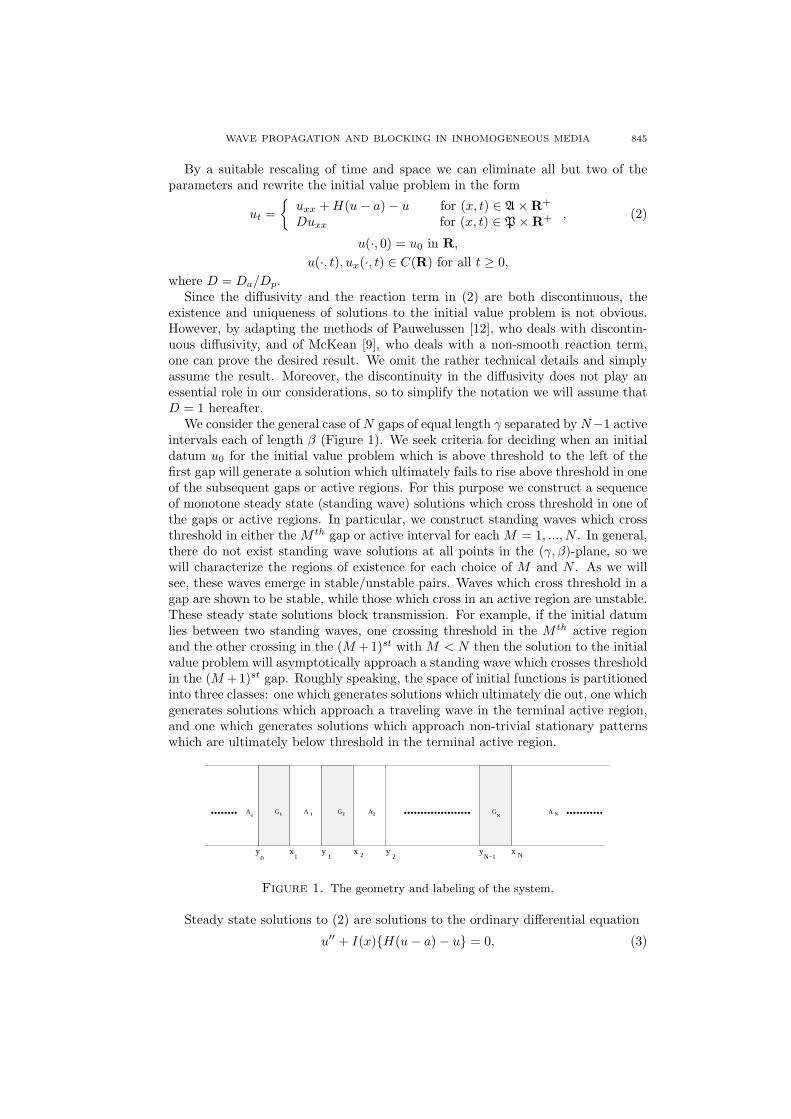
We consider the general case of N gaps of equal length γ separated by N−1 activeintervals each of length β (Figure 1). We seek criteria for deciding when an initialdatum u0 for the initial value problem which is above threshold to the left of thefirst gap will generate a solution which ultimately fails to rise above threshold in oneof the subsequent gaps or active regions. For this purpose we construct a sequenceof monotone steady state (standing wave) solutions which cross threshold in one ofthe gaps or active regions. In particular, we construct standing waves which crossthreshold in either the M th gap or active interval for each M = 1, ..., N . In general,there do not exist standing wave solutions at all points in the (γ, β)-plane, so wewill characterize the regions of existence for each choice of M and N . As we willsee, these waves emerge in stable/unstable pairs. Waves which cross threshold in agap are shown to be stable, while those which cross in an active region are unstable.These steady state solutions block transmission. For example, if the initial datumlies between two standing waves, one crossing threshold in the M th active regionand the other crossing in the (M +1)st with M < N then the solution to the initialvalue problem will asymptotically approach a standing wave which crosses thresholdin the (M +1)st gap. Roughly speaking, the space of initial functions is partitionedinto three classes: one which generates solutions which ultimately die out, one whichgenerates solutions which approach a traveling wave in the terminal active region,and one which generates solutions which approach non-trivial stationary patternswhich are ultimately below threshold in the terminal active region.
G A G A G A....................1 2 2 N N1 ................... A0
y0
x1
y x y2 21y x
N−1 N
Figure 1. The geometry and labeling of the system.
Steady state solutions to (2) are solutions to the ordinary differential equation
u′′ + I(x){H(u− a)− u} = 0, (3)

846 D.G. ARONSON, N.V. MANTZARIS AND HANS OTHMER
where
I(x) ={
0 if x ∈ P1 if x ∈ A
.
In the phase plane, i.e., the (u, u′)-plane, there are rest points at O = (0, 0) andP = (1, 0), both of which are saddles. We assume throughout that a ∈ (0, 1/2).It is easy to show using first integrals that the stable and unstable manifolds of Ocoincide and form a homoclinic loop in the right half plane. The part of the loopin the fourth quadrant is given by
Σ1 : u′ = −u for 0 ≤ u ≤ a
Σ2 : u′ = −√
u2 − 2u + 2a for u > a.
The branch in the fourth quadrant of the unstable manifold associated to P is givenby
Σ3 : u′ = u− 1 for 0 ≤ u ≤ 1.
These manifolds are shown in Figure 2. The steady state solutions we seek aremonotone standing wave solutions which correspond in the phase plane to hetero-clinic orbits from P to O.
Figure 2. The phase plane for the two-gap problem with γ > γ∗ ≡a−1 − 2.
Although our construction of the standing wave solutions is analytic, in the caseof two gaps it is possible to give a rather simple geometric construction which hasthe virtue of clearly displaying the admissible relationships between the lengthsγ and β. We carry this out in Section 2. In Section 3 we turn to the generalcase N ≥ 1 and carry out the formal construction of the standing wave solutionswhich cross the threshold value in the M th gap for M = 1, ..., N . We make thisconstruction rigorous in Section 4 by imposing the necessary constraints. We alsoexplore the consequences of these constraints in determining the bifurcation curvesand delineating the (γ, β) regions for the existence of standing waves. In Section 5we investigate monotonicity properties with respect to M and N of the initial slopeof a monotone standing wave solution which crosses threshold in the M th gap ofan N gap configuration. Standing waves which cross threshold in active regions areconstructed in Section 6. The stability and instability of the various standing wavesis studied in Section 7 using an extension of the comparison result of Pauwelussen

WAVE PROPAGATION AND BLOCKING IN INHOMOGENEOUS MEDIA 847
[12] and the convergence results of Aronson & Weinberger [1, 2]. In that Sectionwe also discuss the pattern formation induced by the presence of gaps. Finally, inSection 8 we summarize our results and discuss various possible extensions.
3. The geometric construction for the two-gap problem. We consider theproblem of constructing monotone standing waves in the presence of two gaps. Weseek a C1 solution to
u′′ + H(u− a)− u = 0 for x ∈ (−∞, 0) ∪ (γ, γ + β) ∪ (2γ + β,∞) (4)
andu′′ = 0 on (0, γ) ∪ (γ + β, 2γ + β). (5)
Since standing waves do not exist for all points in the (γ, β)-plane we proceed byfixing the gap length γ and determining the admissible values of the active regionlength β and the slope −u∗ at x = 0.
To begin with we fix
γ > γ∗ ≡ 1a− 2. (6)
Integrating (4) with a given value of u′ corresponds to traversing a horizontal seg-ment of length γ |u′| in the phase plane. The curves Γ1, Γ2 and Γ3 in Figure 2 showthe locus of phase points at a distance γ |u′| from Σ1,Σ2, and Σ3 respectively. Thuseach point on Γj is the endpoint of a trajectory of (4) whose other endpoint lies onΣj for j = 1, 2, 3 . The heteroclinic orbits we seek are constructed from segmentsof the manifolds Σ1, Σ2 and Σ3, horizontal segments which are trajectories of (4),and curved segments which are trajectories of (4). These curved segments join Γ3
to Γ1 or to Γ2, and determine the admissible values of β corresponding to the givenvalue of γ.
The phase points
Qj ≡{
Γ3 ∩ Σj for j = 1, 2Γ3 ∩ Γj−2 for j = 3, 4
andQa ≡ Γ3 ∩ {u = a}
play a crucial role in determining the admissible values of β and u∗. Define thenumbers uj for j = 1, .., 4 by
Qj ≡ (1− (1 + γ)uj ,−uj)
andua ≡ 1− a
1 + γ.
Thena > u1 > ua > u2 > u3 > u4 > 0.
For 0 < u∗ < u4, where (1 − u∗,−u∗) ∈ Σ3, there are two families of heteroclinicorbits. One of these consists of orbits which cross threshold in the terminal activeregion, e.g., PABCDEO in Figure 2. The curved segment BC represents a tra-jectory of (4) and determines an admissible active region length β. As u∗ ↘ 0, BCapproaches Σ3 and β ↗∞. As u∗ ↗ u4, BC collapses to the point Q4 and β ↘ 0.There are no heteroclinic orbits which cross threshold in the terminal active regionfor u ≥ u4.
Heteroclinic orbits in the other family cross threshold in the second gap. Theyexist for 0 < u∗ < u4 and persist beyond u∗ = u4 for u4 ≤ u∗ < u3. An example is

848 D.G. ARONSON, N.V. MANTZARIS AND HANS OTHMER
PABFGO in Figure 2. For these orbits the length β is determined by the curvedsegment BF with β ↘ 0 as u∗ ↗ u3 and β ↗ ∞ as u∗ ↘ 0. The leftmost twocurves in Figure 3 show β as a function of u∗ for these two families of heteroclinicorbits.
Figure 3. The (u, β)-plane for the two-gap problem with thresholda = 0.45 and gap length γ = 0.3 > γ∗ = 2/9. Here −u is the initialslope and β is the length of the intervals in the active region. For points(γ, β) on the curve labeled a (c) the corresponding standing wave solutioncrosses threshold in the active region A2 (A1). For points (γ, β) on thecurve labeled b (d) the corresponding standing wave solution crossesthreshold in the gap G2 (G1). The point labeled P is the minimum point
(ua, βa).
For u2 < u∗ < ua there is a family of heteroclinic orbits which cross thresholdin the active region A1, e.g., PHIJKLO in Figure 2. The admissible values ofβ are determined by the trajectory IJK of (4) with β ↗ ∞ as u∗ ↘ u2. Forua < u∗ < u1 there is a family of heteroclinic orbits which cross threshold in thefirst gap, e.g., PMNKLO. Here the admissible values of β are determined bythe trajectory NK of (4) with β ↗ ∞ as u∗ ↗ u1. When u∗ → a the twofamilies discussed here coalesce and there is a minimal value of β determined by thetrajectory JK. The two rightmost curves in Figure 3 show β as a function of u∗ forthese two families. Note that the curves intersect at the point (u∗, β) = (ua, βa),where βa is the minimal allowable active region length for the given gap length γ.The point (ua, βa) is a bifurcation point in the sense that there are two distinctsolution branches in its neighborhood.
When γ = γ∗ the intersection of Γ3 and Σ1 ∪ Σ2 is the single point (a,−a),while for γ < γ∗ the intersection is empty. Thus there are no monotone standingwaves which cross threshold in either the terminal active region or the second gapfor γ ≤ γ∗. However if
12γ∗ < γ < γ∗
then Γ1 and Γ2 intersect the line u′ = −a in a point C (cf. Figure 4) whose u-coordinate lies in the interval (a/2, 1− a). The trajectory of (4) which starts at Cintersects Γ3 in a point
B ≡ (1− (1 + γ)ub,−ub)
where ub ∈ (0, a) with ub ↘ 0 as γ → γ∗ and ub ↗ a as γ → 12γ∗.

WAVE PROPAGATION AND BLOCKING IN INHOMOGENEOUS MEDIA 849
O P
Σ1
AB
CD
EF
G
I
H
J
ΓΣ
Γ
Σ
1
2
2
3
Γ3
Q
Q
3
4
−u
−u
−u
−a
a
b
3
4
Figure 4. The phase plane for the two-gap problem with γ∗2
< γ < γ∗.
For ub < u∗ < u4 there is a family of heteroclinic orbits which cross thresholdin the terminal active region, e.g., PEFGHDO in Figure 4. For these orbits thelength β of the active region is determined by the curve FG with β ↘ 0 as u∗ ↗ u4.There are no heteroclinic orbits which cross threshold in the terminal active regionfor u∗ ≥ u4.
For u3 < u∗ < ub there is a family of heteroclinic orbits which cross threshold inthe second gap, e.g., PEFIJO in Figure 4. For these trajectories the length β ofthe active region is determined by the curve FI with β ↘ 0 as u∗ ↘ u3. There areno heteroclinic orbits crossing threshold in the second gap for u∗ ≤ u3.
The two families coincide at u∗ = ub (PABCDO in Figure 4) and there is amaximal value of β = βb (determined by the curve BC) . Figure 5 shows β as afunction of u∗ for these two families. These curves intersect in a bifurcation pointat (u∗, β) = (ub, βb).
Figure 5. The (u, β)-plane for the two-gap problem with thresholda = 0.45 and gap length γ = 0.15 ∈ ( 1
2γ∗, γ∗). Here −u is the initial
slope and β is the length of the intervals in the active region. For points(γ, β) on the curve labeled a (b) the corresponding standing wave solutioncrosses threshold in the active region A2 (the gap G2). The point labeledP is the maximum point (ub, βb).
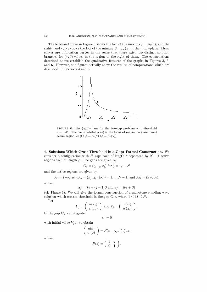
850 D.G. ARONSON, N.V. MANTZARIS AND HANS OTHMER
The left-hand curve in Figure 6 shows the loci of the maxima β = βb(γ), and theright-hand curve shows the loci of the minima β = βa(γ) in the (γ, β)-plane. Thesecurves are bifurcation curves in the sense that there exist two distinct solutionbranches for (γ, β)-values in the region to the right of them. The constructionsdescribed above establish the qualitative features of the graphs in Figures 3, 5,and 6. However, the figures actually show the results of computations which aredescribed in Sections 4 and 6.
Figure 6. The (γ, β)-plane for the two-gap problem with thresholda = 0.45. The curve labeled a (b) is the locus of maximum (minimum)active region length β = βb(γ) (β = βa(γ)).
4. Solutions Which Cross Threshold in a Gap: Formal Construction. Weconsider a configuration with N gaps each of length γ separated by N − 1 activeregions each of length β. The gaps are given by
Gj = (yj−1, xj) for j = 1, ..., N
and the active regions are given by
A0 = (−∞, y0), Aj = (xj , yj) for j = 1, ..., N − 1, and AN = (xN ,∞),
wherexj = jγ + (j − 1)β and yj = j(γ + β)
(cf. Figure 1). We will give the formal construction of a monotone standing wavesolution which crosses threshold in the gap GM , where 1 ≤ M ≤ N.
Let
Uj =(
u(xj)u′(xj)
)and Vj =
(u(yj)u′(yj)
).
In the gap Gj we integrateu′′ = 0
with initial value Vj−1 to obtain(
u(x)u′(x)
)= P (x− yj−1)Vj−1,
where
P (z) =(
1 z0 1
).
WAVE PROPAGATION AND BLOCKING IN INHOMOGENEOUS MEDIA 851
In particular, at the end of Gj we have
Uj = PVj−1,
where
P = P (γ) =(
1 γ0 1
).
If j < M we are above threshold so that in Aj we integrate
u′′ − u + 1 = 0
with initial value Uj to obtain(u(x)u′(x)
)− ε1 = A(x− xj)(Uj − ε1),
where
A(z) =(
cosh z sinh zsinh z cosh z
)and ε1 =
(10
).
Thus at the end of Aj we have
Vj − ε1 = A(PVj−1 − ε1), (7)
where
A = A(β) =(
cosh β sinhβsinhβ cosh β
).
For the first gap the left-hand endpoint must lie on the unstable manifold of therest point P = (1, 0) in A0. Write
V0 =(
1− u∗
−u∗
).
ThenU1 = PV0 = ε1 − u∗Pε,
where
ε =(
11
),
andV1 − ε1 = −u∗APε. (8)
In view of (8), iteration of (7) yields
VM−1 − ε1 = −u∗(AP )M−1ε,
and crossing GM we find
UM−1 = ε1 − u∗P (AP )M−1ε
since Pε1 = ε1.Since we assume that the threshold u = a is crossed in GM the Heaviside function
in (3) is zero, we proceed by integrating
u′′ − u = 0
across AM to obtainVM = Aε1 − u∗(AP )M ε
andUM+1 = PAε1 − u∗P (AP )M ε.
Continuing in this manner successively applying A and P yields
UN = (PA)N−M ε1 − u∗P (AP )N−1ε

852 D.G. ARONSON, N.V. MANTZARIS AND HANS OTHMER
at the end of the final gap GN . The stable manifold of O is given by u + u′ = 0.Since UN must lie on this manifold we have
0 = εT UN = εT (PA)N−M ε1 − u∗εT P (AP )N−1ε
so that
u∗ = u∗MN =εT (PA)N−M ε1εT P (AP )N−1ε
. (9)
Note that (9) can also be written in the form
u∗MN =εT (PA)N−M ε1
εT (PA)k−1P (AP )N−kεfor k = 1, ..., N. (10)
To simplify (10), we write
(AP )kε=(
fk
gk
), (11)
where
AP =(
cosh(β) sinh(β) + γ cosh(β)sinh(β) cosh(β) + γ sinh(β)
).
Note that f0 = g0 = 1, and that fk and gk are positive for all integers k. Moreover,
fk+1 > fk and gk+1 > gk. (12)
Since
(PA)k =(
0 11 0
) ((AP )k
)T(
0 11 0
)
it follows that
εT (PA)k =(
gk fk
). (13)
Thus we can rewrite (10) as
u∗MN =gN−M
gk−1(fN−k + γgN−k) + fk−1gN−kfor k = 1, ..., N. (14)
Note that (14) implies that
gk−1(fN−k + γgN−k) + fk−1gN−k = gj−1(fN−j + γgN−j) + fj−1gN−j for all k, j.(15)
Once u∗ is known, the monotone standing wave is uniquely determined, at leastformally. In particular
(uu′
)=
ε1 − u∗P (x− yk−1)(AP )k−1ε for x ∈ Gk, k ≤ M
ε1 − u∗A(x− xk)P (AP )k−1ε for x ∈ Ak, k ≤ M − 1
A(x− xk){(PA)k−M ε− u∗P (AP )k−1ε} for x ∈ Ak, M ≤ k ≤ N − 1
P (x− xk){A(PA)k−M ε− u∗(AP )kε} for x ∈ Gk,M ≤ k ≤ N
.
(16)Note that formally the function defined by (16) is a steady state solution on [0, xN ]which crosses threshold in the Mth gap. However, it is not a standing wave unlessu∗ = u∗MN .
WAVE PROPAGATION AND BLOCKING IN INHOMOGENEOUS MEDIA 853
5. Constraints. The derivation of the formulae (14) for u∗MN given in the previoussection is purely formal. Although it is assumed that the threshold is crossed in theM th gap, u∗MN as given by (14) is in fact independent of the value of the thresholdparameter a. Hence there is no guarantee that this crossing actually occurs for anypreassigned value of a. To ensure a crossing we must apply various constrains whichdepend on the actual value of a.
In the gap GM the solution starts at the phase point (1−u∗MNfM−1,−u∗MNgM−1).Since this point must not lie below threshold we must require that 1−u∗MNfM−1 ≥ a,i.e.,
u∗MN ≤ 1− a
fM−1.
Using (13) with L = N −M + 1 this is equivalent to
XMN (γ, β) ≡ (1a− 1)gM−1(fN−M + γgN−M )− fM−1gN−M ≥ 0. (17)
Equality in (17) occurs exactly when the solution crosses threshold at the beginningof the GM or, equivalently, at the end of the AM−1. Moreover, the phase point(1−u∗MNfM−1,−u∗MNgM−1) must lie above the line u′ = −a. Hence we must have−u∗MNgM > −a or
u∗MN <a
gM−1.
An equivalent form of this condition is
YMN (γ, β) ≡ gN−M (fM−1 + γgM−1) + gM−1(fN−M − 1agN−M ) ≥ 0. (18)
In the gap GM the solution ends at the phase point
(1− u∗MN (fM−1 + γgM−1),−u∗MNgM−1).
This point must lie on or to the left of u = a and either on the stable manifold of0 if M = N or to the right of it if M < N . Thus
u∗MNgM−1 ≤ 1− u∗MN (fM−1 + γgM−1) ≤ a (19)
with equality on the left if and only if M = N.The left hand inequality in (19) is always satisfied. To see this observe that, in
view of (14) with k = N −M + 1, this inequality is equivalent to
gM−1(fN−M+1 − gN−M+1) ≥ 0.
Since gk > 0 it suffices to prove that
fk − gk > 0 for all integers k ≥ 1. (20)
We do this by induction. For k = 1
f1 − g1 = γ(coshβ − sinhβ) > 0.
Write
(AP )k =(
m11 m12
m21 m22
),
where the mij > 0. Then fk = m11 + m12, gk = m21 + m22, and we assume thatfk − gk > 0. Now
(AP )k+1 =(m11 coshβ + m21(sinhβ + γ coshβ) m12 cosh β + m22(sinh β + γ cosh β)m11 sinhβ + m22(coshβ + γ sinhβ) m12 sinh β + m22(coshβ + γ sinh β)
)
854 D.G. ARONSON, N.V. MANTZARIS AND HANS OTHMER
so thatfk+1 − gk+1 = (fk − gk + γgk) (cosh β − sinhβ) > 0,
which proves the assertion.The right hand inequality in (19) is equivalent to
u∗MN >1− a
fM−1 + γgM−1
or
ZMN (γ, β) ≡ gN−M (fM−1 + γgM−1) + (1− 1a)fN−MgM−1 ≥ 0. (21)
Note that equality in (21) occurs exactly when the solution crosses threshold at theend of GM or equivalently at the beginning of AM .
For the existence of a monotone standing wave solution which crosses thresholdin the M th gap it is necessary and sufficient that (γ, β) be such that (17), (18), and(21) are simultaneously satisfied. In view of (18) and (21) we have
YMN = ZMN +1agM−1(fN−M − gN−M ).
Since YNN = 0 and ZMN = 0 coincide, it follows from (20) that
YMN ≥ ZMN with equality only for M = N.
Therefore YMN ≥ 0 whenever ZMN ≥ 0, and in particular, (18) is automaticallysatisfied whenever (21) holds. Thus the condition (18) is redundant. The regionin the (γ, β)−plane where (17) and (21) both hold is delineated by the sets whereXMN (γ, β) and ZNM (γ, β) vanish. The coincidence of YNN = 0 and ZNN = 0means that the phase point at the end of the N th gap has coordinates (a,−a).
In the two-gap case discussed in Section 2, the curves β = βa(γ) and β = βb(γ)in Figure 6 are, respectively, the curves Z12 = 0 and Z22 = 0. Figure 7 shows thecurves XM5 = 0 and ZM5 = 0 for two different values of the threshold parameter aand for various values of M ∈ {1, ..., 5}. As we noted above, the curves XMN = 0and ZMN = 0 describe the loci of points in the (γ, β)-plane where the crossing ofthe threshold occurs at the intersection of an active and a passive region. As inthe two-gap case, we expect these points to be bifurcation points where branches ofsolutions crossing in an active and in a passive region meet. This will be discussedin Section 6.
We investigate the sets where XMN (γ, β) = 0 and ZNM (γ, β) = 0. Since
A(β)P (0) =(
cosh β sinhβsinhβ cosh β
)
we have (fk(0, β)gk(0, β)
)= (cosh β + sinh β)ke.
ThereforeXMN (0, β) = γ∗(cosh β + sinh β)N−1 > 0 (22)
andZNM (0, β) = −γ∗(coshβ + sinh β)N−1 < 0, (23)
where
γ∗ =1a− 2.

WAVE PROPAGATION AND BLOCKING IN INHOMOGENEOUS MEDIA 855
Figure 7. (a) The (γ, β)-plane for the five-gap problem with thresholda = 0.45. The curve labeled a is X45 = 0, b is X55 = 0, c is Z15 = 0, dis Z25 = 0, e is Z35 = 0, f is Z45 = 0, and g is Z55 = 0. For a = 0.45,XM5 6= 0 in the first quadrant for M = 1, 2,or 3. (b) The (γ, β)-planefor the five-gap problem with threshold a = 0.4. The curve labeled a isX55 = 0, b is Z15 = 0, c is Z25 = 0, d is Z35 = 0, e is Z45 = 0, and f isZ45 = 0. For a = 0.4, XM5 6= 0 in the first quadrant for M = 1, 2, 3 or
4.
For fixed β and γ À 1
A(β)P (γ) ∼ γ
(0 cosh β0 sinh β
)
so that (fk(γ, β)gk(γ, β)
)∼ γk (sinhβ)k−1
(cosh βsinhβ
)as γ →∞.
It follows that
XMN (γ, β) ∼ (1a− 1)γN (sinhβ)N−1 > 0 as γ →∞ (24)
andZNM (γ, β) ∼ γN (sinh β)N−1
> 0 as γ →∞. (25)
Since
(A(0)P (γ))k =(
1 γ0 1
)k
=(
1 kγ0 1
)
we have (fk(γ, 0)gk(γ, 0)
)=
(1 + kγ
1
).
HenceXMN (γ, 0) = γ∗ +
γ
a(Na −M + 1)
andZMN (γ, 0) = −γ∗ − γ
a(Na −M),
whereNa ≡ (1− a)N.
We conclude that
XMN (γ, 0){
> 0 if 0 ≤ γ < γM−1,N
< 0 if γ > γM−1,N(26)

856 D.G. ARONSON, N.V. MANTZARIS AND HANS OTHMER
and
ZMN (γ, 0){
< 0 if 0 ≤ γ < γMN
> 0 if γ > γMN, (27)
where
γMN =
+∞ if M ≤ Na1− 2a
M −Naif M > Na
.
In Appendix A we show that
XMN (γ, β) ∼ (γ∗ + (1a− 1)γ)(2 + γ)N−1
(eβ
2
)N−1
> 0 as β →∞, (28)
ZMN (γ, β) ∼ (2 + γ)N−1(γ − γ∗)(
eβ
2
)N−1
as β →∞, (29)
and
ZMN (γ∗, β) ∼ γ∗(2 + γ∗)N−2 e(N−3)β
2N−2×
1 if M = N(2− 1
a
)< 0 if 2 ≤ M ≤ N − 1
(1− 1
a
)< 0 if M = 1
(30)as β →∞.
¿From (23) and (25) we see that for each β > 0 there is at least one root ofZMN (γ, β) = 0 in R+. Let γ = ζMN (β) denote the smallest such root. Genericallywe would expect the graph of γ = ζMN (β) to consist of a number of disjoint arcs.However, all of our numerical studies (cf. Figure 7) indicate that it is a smoothcurve and that there are no additional roots in the first quadrant. To simplify thediscussion we will assume that this is indeed the case.
We can say more about the set ZNN = 0 for large N . At the end of GN we have(
a−a
)= ε1 − u∗NN (PA)N−1Pε,
where u∗NN (γ, β) is defined by
u∗NN =1− a
εT1 (PA)N−1Pε
.
Let
ε2 =(
01
).
The equationa = u∗NN εT
2 (PA)N−1Pε
establishes a relationship between γ and β. In particular
1a− 1 =
εT1 (PA)N−1Pε
εT2 (PA)N−1Pε
.
The eigenvalues of PA are
λj =12
(2 cosh β + γ sinhβ + (−1)j
√(2 cosh β + γ sinhβ)2 − 4
)for j = 1, 2
WAVE PROPAGATION AND BLOCKING IN INHOMOGENEOUS MEDIA 857
and the corresponding eigenvalues are
vj =
λ2 − cosh β
sinhβ1
.
Note that λ1λ2 = 1 and 0 < λ1 < 1 < λ2. Write
Pε = c1v1 + c2v2,
where the cj depend on γ, β, and N . Then
(PA)N−1Pε = c1λN−11 v1 + c2λ
N−12 v2
and1a− 1 =
c1λN−11 εT
1 v1 + c2λN−12 εT
1 v2
c1λN−11 εT
2 v1 + c2λN−12 εT
2 v2
.
Therefore1a− 1 =
λ2 − cosh β
sinhβ+O(ρN−1),
where ρ = λ1/λ2 < 1. It follows that
γNN (β) =α2 − 1
α + coth β+O(ρN−1),
where α =1a− 1. In particular, the limiting position of γ = γNN (β) is given by
γ∞(β) = limN→∞
γNN (β) =α2 − 1
α + coth β
and for each fixed β the convergence is exponential. Moreover,
limβ→∞
γ∞(β) = γ∗.
Figure 8 is a schematic representation of the first quadrant of the (γ, β)−planeas a finite rectangle. In this representation the upper and right hand sides of therectangle represent β = ∞ and γ = ∞ respectively. According to (23) and (27),if M ≤ Na then ZMN < 0 on the left hand and lower boundaries of the rectangle,and this is indicated by the dashed lines. From (25) we see that ZMN > 0 on theright hand boundary and this is indicated with a heavy solid line. On the top ofthe rectangle, in view of (27), ZMN < 0 for γ < γ∗ and > 0 for γ > γ∗. Finally,from (28) we see that ZMN (γ∗, β) < 0 for β → ∞. The curve γ = ζMN (β) mustcontain the points α = (γ∗,∞) and ω = (∞, 0) where ZMN changes sign and mustapproach α from the right, as indicated in the figure. The part of the curve betweenthese points is drawn to agree with our numerical observations (cf. Figure 7).
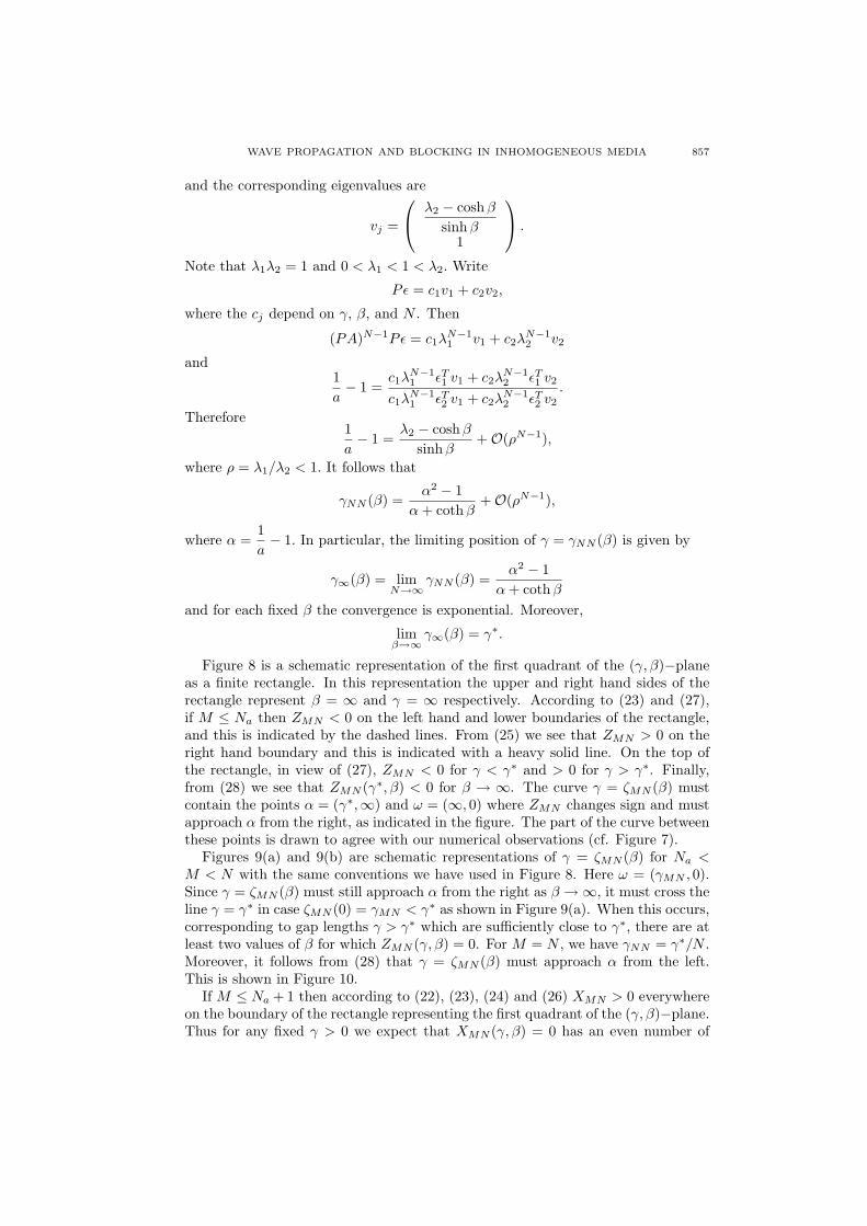
Figures 9(a) and 9(b) are schematic representations of γ = ζMN (β) for Na <M < N with the same conventions we have used in Figure 8. Here ω = (γMN , 0).Since γ = ζMN (β) must still approach α from the right as β →∞, it must cross theline γ = γ∗ in case ζMN (0) = γMN < γ∗ as shown in Figure 9(a). When this occurs,corresponding to gap lengths γ > γ∗ which are sufficiently close to γ∗, there are atleast two values of β for which ZMN (γ, β) = 0. For M = N , we have γNN = γ∗/N .Moreover, it follows from (28) that γ = ζMN (β) must approach α from the left.This is shown in Figure 10.
If M ≤ Na + 1 then according to (22), (23), (24) and (26) XMN > 0 everywhereon the boundary of the rectangle representing the first quadrant of the (γ, β)−plane.Thus for any fixed γ > 0 we expect that XMN (γ, β) = 0 has an even number of

858 D.G. ARONSON, N.V. MANTZARIS AND HANS OTHMER
β
γγ ω
α
γ=ζ ΜΝ (β)
∗
Figure 8. Schematic representation of the (γ, β)-plane for M ≤ Nshowing ZMN = 0.
β
γγ
α
γ=ζ ΜΝ (β)
∗ω
(a)
β
γγ
α
γ=ζ ΜΝ (β)
∗ ω
(b)
Figure 9. Schematic representation of the (γ, β)-plane for Na < M <N showing ZMN = 0. There are two cases: (a) if γMN < γ∗ then thecurve γ = ζMN (β) lies to the left of the line γ = γ∗ for all sufficientlysmall β ≥ 0 and to the right of it for all sufficiently large values of β.(b) if γMN > γ∗ then the curve γ = ζMN (β) lies to the right of the lineγ = γ∗ for all sufficiently small β ≥ 0 and for all sufficiently large valuesof β.
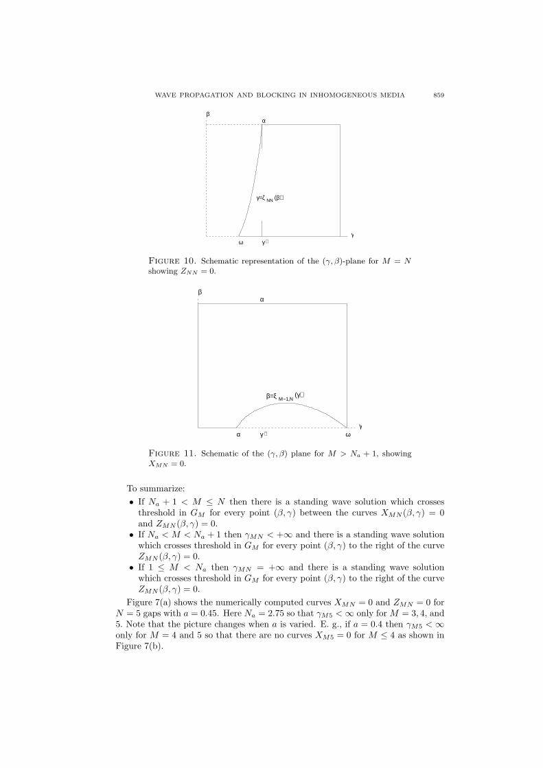
roots. In fact our numerical studies show that there are no roots in this case. Onthe other hand, for M > Na + 1, it follows from (26) that XMN (γ, 0) < 0 betweenα = (γM−1,N , 0) and ω = (0,∞). In particular, there is a least positive rootβ = ξM−1,N (γ) whose graph joins α to ω. Again our numerical studies indicatethat this graph is a smooth curve joining α to ω as shown in Figure 11.
WAVE PROPAGATION AND BLOCKING IN INHOMOGENEOUS MEDIA 859
β
γγ
α
∗ω
γ=ζ ΝΝ (β)
Figure 10. Schematic representation of the (γ, β)-plane for M = Nshowing ZNN = 0.
β
γγ
α
∗α ω
β=ξ Μ−1,Ν(γ)
Figure 11. Schematic of the (γ, β) plane for M > Na + 1, showingXMN = 0.
To summarize:• If Na + 1 < M ≤ N then there is a standing wave solution which crosses
threshold in GM for every point (β, γ) between the curves XMN (β, γ) = 0and ZMN (β, γ) = 0.
• If Na < M < Na + 1 then γMN < +∞ and there is a standing wave solutionwhich crosses threshold in GM for every point (β, γ) to the right of the curveZMN (β, γ) = 0.
• If 1 ≤ M < Na then γMN = +∞ and there is a standing wave solutionwhich crosses threshold in GM for every point (β, γ) to the right of the curveZMN (β, γ) = 0.
Figure 7(a) shows the numerically computed curves XMN = 0 and ZMN = 0 forN = 5 gaps with a = 0.45. Here Na = 2.75 so that γM5 < ∞ only for M = 3, 4, and5. Note that the picture changes when a is varied. E. g., if a = 0.4 then γM5 < ∞only for M = 4 and 5 so that there are no curves XM5 = 0 for M ≤ 4 as shown inFigure 7(b).

860 D.G. ARONSON, N.V. MANTZARIS AND HANS OTHMER
6. Monotonicity. The initial slope u∗MN (γ, β) which yields a monotone standingwave solution crossing threshold in the M th gap in an N gap configuration hascertain monotonicity properties with respect to the indices M and N . Specifically,we have
u∗1N > u∗2N > · · · > u∗NN (31)and
u∗MN > u∗MN+1. (32)An immediate consequence of (31) and (32) is
u∗MN > u∗M+1,N+1. (33)
According to (14) with k = 1
u∗MN =gN−M
fN−1 + (1 + γ)gN−1
and (31) is an immediate consequence of the monotonicity of the gk with respectto the index (12). To prove (32) we use (14) with k = M to write (32) in the form
gN−M
gM−1(fN−M + γgN−M ) + fM−1gN−M>
gN+1−M
gM−1(fN+1−M + γgN+1−M ) + fM−1gN+1−M.
Thus (32) is equivalent to
QMN ≡ gN−MfN+1−M − gN+1−MfN−M > 0. (34)
If we write
(AP )N−M =(
a11 a12
a21 a22
)
thenfN−M = a11 + a12 and gN−M = a21 + a22.
Note that the aij > 0. Since
(AP )N−M+1 =(
a11 cosh β + a12 sinhβ a11(sinhβ + γ cosh β) + a12(coshβ + γ sinh β)a21 cosh β + a22 sinhβ a21(sinhβ + γ cosh β) + a22(coshβ + γ sinh β)
)
it follows that
fN−M+1 = a11(sinh β + (1 + γ) cosh β) + a12(coshβ + (1 + γ) sinh β)
and
gN−M+1 = a21(sinhβ + (1 + γ) cosh β) + a22(coshβ + (1 + γ) sinh β).
Substituting in (34) yields
QMN = γ(coshβ − sinhβ) det{(AP )N−M
}.
Howeverdet
{(AP )N−M
}= {detAP}N−M
and
detAP =∣∣∣∣
coshβ sinh β + γ cosh βsinhβ cosh β + γ sinh β
∣∣∣∣ = cosh2 β − sinh2 β = 1.
ThereforeQMN = γ(coshβ − sinh β) > 0.
In Figure 7 the curves ZMN = 0 lie to the right of the curves ZM+1,N = 0. Weshow here that this monotonicity is a general property. In particular, we show that
ZMN (γ, β) ≥ 0 implies ZM+1,N (γ, β) > 0 (35)

WAVE PROPAGATION AND BLOCKING IN INHOMOGENEOUS MEDIA 861
whenever both are defined. Using (15) we can write the condition ZMN ≥ 0 in theform
fN−1 + (1 + γ)gN−1 ≥ 1afN−MgM−1. (36)
Similarly
ZM+1,N = fN−1 + (1 + γ)gN−1 − 1afN−M−1gM
so that (36) implies that
ZM+1,N ≥ 1a
(fN−MgM−1 − fN−M−1gM ) .
Therefore the sign of ZM+1,N is determined by the sign of
QM+1,N ≡ fN−MgM−1 − fN−M−1gM .
By (11)
QM+1,N = εT1 (AP )N−M εεT
2 (AP )M−1ε− εT1 (AP )N−M−1εεT
2 (AP )M ε
which we rewrite as
QM+1,N = εT1 (AP )N−M−1R (AP )M−1ε,
where
R = APεεT2 − εεT
2 AP =( − sinhβ sinhβ + γ(coshβ − sinhβ− sinhβ sinhβ
).
It is not difficult to verify that
APRAP = R. (37)
Suppose first that M ≤ N/2. Then it follows from (37) that
QM+1,N = εT1 (AP )N−2MRε = γ(coshβ − sinhβ)a11 > 0,
where (AP )N−2M = (aij) and all of the aij are positive..If M > N/2 we have
QM+!,N = εT1 R(AP )2M−N ε,
which, in view of (37), we rewrite as
QM+1,N = εT1 {(AP )2M−N}−1Rε. (38)
Let (AP )2M−N = (bij), where all of the bij are positive. Therefore, sincedet (AP )2M−N = 1 and
(AP )−1 =(
b22 −b21
−b12 b11
),
it follows from (38) that
QM+1,N = γ(coshβ − sinhβ)b22 > 0.
This completes the proof of (35).In a similar manner we can show that
XMN (γ, β) ≥ 0 implies that XM−1,N (γ, β) > 0.
We omit the details.

862 D.G. ARONSON, N.V. MANTZARIS AND HANS OTHMER
7. Solution crossing threshold in an active region. We now consider theconstruction of monotone standing wave solutions which cross threshold in the M th
active region in an N gap configuration, where M ∈ {1, 2, ..., N − 1}. This con-struction is considerably more complicated than the corresponding construction forsolutions which cross threshold in a gap since now we have to deal explicitly withthe nonlinearity of the problem.
To construct a standing wave solution which crosses threshold in the M th activeregion AM , we fix a δ ∈ [0, 1], integrate the super-threshold equation u′′−u+1 = 0a distance δβ until u reaches the value a, and then integrate the sub-thresholdequation u′′−u = 0 a distance β(1− δ) to complete the traversal of AM . This is, ofcourse, not possible for every choice of γ, β, and δ, but we will derive the admissible(γ, β)-set for any given δ. We will use the notation and conventions of Sections 3and 4 .
If the initial slope is −v∗, then at the end of the gap GM we have
UM−1 = ε1 − v∗P (AP )M−1ε,
where A = A(β) and P = P (γ). Assuming that the point UM−1 lies between thestable manifold Σ2 and the line u = a, follow the trajectory of u′′ − u + 1 = 0 for adistance δβ to obtain
(au′
)= ε1 − v∗A(δβ)P (AP )M−1ε. (39)
In particular, γ, β, δ, and v∗ are constrained by the condition
a = 1− v∗εT1 A(δβ)P (AP )M−1ε. (40)
In addition, δ is constrained by the condition
0 ≤ δ ≤ 1. (41)
Continue by integrating the sub-threshold equation u′′−u = 0 for a distance β(1−δ)to obtain
VM = A((1− δ)β)ε1 − v∗A((1− δ)β)A(δβ)P (AP )M−1ε.
Finally proceeding as in Section 3, we arrive at
0 = εT (PA)N−M−1PA((1− δ)β)ε1 (42)
−v∗εT P (AP )N−M−1A((1− δ)β)A(δβ)P (AP )M−1ε.
(40) and (42) yield two expressions for the critical slope −v∗, and since theymust agree we led to the condition
VMN (γ, β; δ) ≡ (1− a){εT (PA)N−M−1PA((1− δ)β)A(δβ)P (AP )M−1ε
}−{εT (PA)N−M−1PA((1− δ)β)ε1
}{εT1 A(δβ)P (AP )M−1ε
}= 0
for the existence of a heteroclinic orbit which crosses threshold in the M th activeregion. Since A(0) = I,
VMN (γ, β; 0) = −aZMN (γ, β)
andVMN (γ, β; 1) = −aXM+1,N (γ, b),
where XM+1,N and ZMN are defined in Section 4.

WAVE PROPAGATION AND BLOCKING IN INHOMOGENEOUS MEDIA 863
For each fixed δ ∈ [0, 1] we can compute the set VMN (γ, β; δ) = 0 in the (γ, β)-plane. Several examples are shown in Figure 12. If
1 ≤ M ≤ Na ≡ (1− a)N
then for eachδ ∈ [0, a)
the set VMN (γ, β; δ) = 0 is a smooth curve in the (γ, β)-plane of the form γ = Γ(β; δ)with asymptotes at β = 0 and β = β∗(δ), where β∗ is the unique positive solutionto
tanh((1− δ)β) tanh(δβ) =a− δ
1− a− δ. (43)
These curves fill out the region in the (γ, β)-plane to the right of ZMN (γ, β) =
−1aVMN (γ, β; 0) = 0. The set VMN (γ, β; δ) = 0 is empty for δ ≥ a. An example is
given in Figure 12(a).
Figure 12. The (γ, β)-plane for the three-gap problem with a = 0.45.(a) The curves V13(γ, β; δ) = 0 are shown (from left to right) for δ =0, 0.1, ..., 0.4. Here Na = 1.65 > M = 1. (b) The curves V33(γ, β; δ) =0 are shown (from left to right) for δ = 0.440, 0.441, ..., 0.445. HereNa + 1 = 2.65 < M = 3. Note that for the range of γ in this figureV33(γ, β; 0.445) = 0 shows two components.
The formula (43) is derived by considering the asymptotic behavior of VMN forγ À 1. Observe that
(PA)N−M−1 ∼ γN−M−1(sinh(β))N−M−2
(sinh(β) cosh(β)
0 0
),
(AP )M−1 ∼ γM−1(sinh(β))M−2
(0 cosh(β)0 sinh(β)
),
and
P ∼ γ
(0 10 0
)
as γ →∞ . Therefore
VMN (γ, β; δ) ∼ γN (sinh(l))N−2{(1− a) cosh((1− δ)β) sinh(δβ) (44)
−a sinh((1− δ)β) cosh(δβ)}as γ →∞. It follows from (44) that VMN ∼ 0 as γ →∞ if either γN (sinh(l))N−2 →0 as γ →∞ or (43) has a solution β = β∗ > 0.
864 D.G. ARONSON, N.V. MANTZARIS AND HANS OTHMER
ForNa < M ≤ N
the situation is somewhat different because in addition to the curve ZMN = 0 thereis also the curve XM+1,N = 0, and the sets VMN = 0 fill out the region betweenthem. For each
δ ∈ [a, 1]
the set VMN (γ, β; δ) = 0 is a curve starting at (γMN , 0) and approximatingXM+1,N (γ, β) = 0 as γ →∞. For each
δ ∈ (0, a)
the set VMN (γ, β; δ) = 0 is a curve starting at (γMN , 0) which asymptotes at β =β∗(δ) for γ → ∞. For δ very close to a this curve stays close to XM+1,N = 0 forvery large value of γ before switching to it’s asymptotic behavior. An example isgiven in Figure 12 (b). (Our numerical evidence is not sufficiently sharp to ruleout the possibility that for δ near a the set VMN = 0 possesses two components;one which approximates XM+1,N = 0 and another which asymptotes at β = 0 andβ = β∗.)
We can also use (40) and (41) to study the relationship between the active regionlength β and the critical initial slope −v∗. Using (11) and the fact that cosh(l)2 −sinh(l)2 = 1 we rewrite (40) in the form
1− a
v− gM−1 sinh(δβ) = (fM−1 + γgM−1)
√1 + sinh(δβ)2,
where we have written v in place of v∗. This is a quadratic equation for sinh(δβ)which we solve to obtain
δ∗(γ, β, v) ≡ 1β
arcsin h
{−(1− a)gM−1 + (fM−1 + γgM−1)
√(1− a)2 − v2pM−1
vpM−1
},
where
pM−1 = pM−1(γ, β) ≡ (fM−1(γ, β) + γgM−1(γ, β))2 − gM−1(γ, β)2.
In view of the constraint (41) we define
δ = δ(γ, β, v) ≡
0 if δ∗(γ, β, v) < 0δ∗(γ, β, v) if 0 ≤ δ∗(γ, β, v) ≤ 11 if δ∗(γ, β, v) > 1
. (45)
Using the formula (45) in (42) we obtain a relationship between γ, β, and thecritical initial slope −v. For each fixed γ this is an implicit relationship betweenv and the active region length β , and we can plot the resulting curves in the(v, β)-plane. Figures 3 and 5 show the results of this computation for a two-gapconfiguration. Figure 13 shows some results for the case of three gaps. Note that byusing (45) we account for threshold crossings not only in AM , but also in GM whenδ = 0 and in GM+1 when δ = 1. Thus the curves which we generate in this mannershow the bifurcations which occur when the threshold is crossed at the intersectionof an active and a passive region.
There remains to be considered the case in which the standing wave solutioncrosses threshold in the terminal active region AN . At the end of the N th gap GN ,since threshold has not yet been crossed, we have
UN−1 = ε1 − uP (AP )N−1ε. (46)
WAVE PROPAGATION AND BLOCKING IN INHOMOGENEOUS MEDIA 865
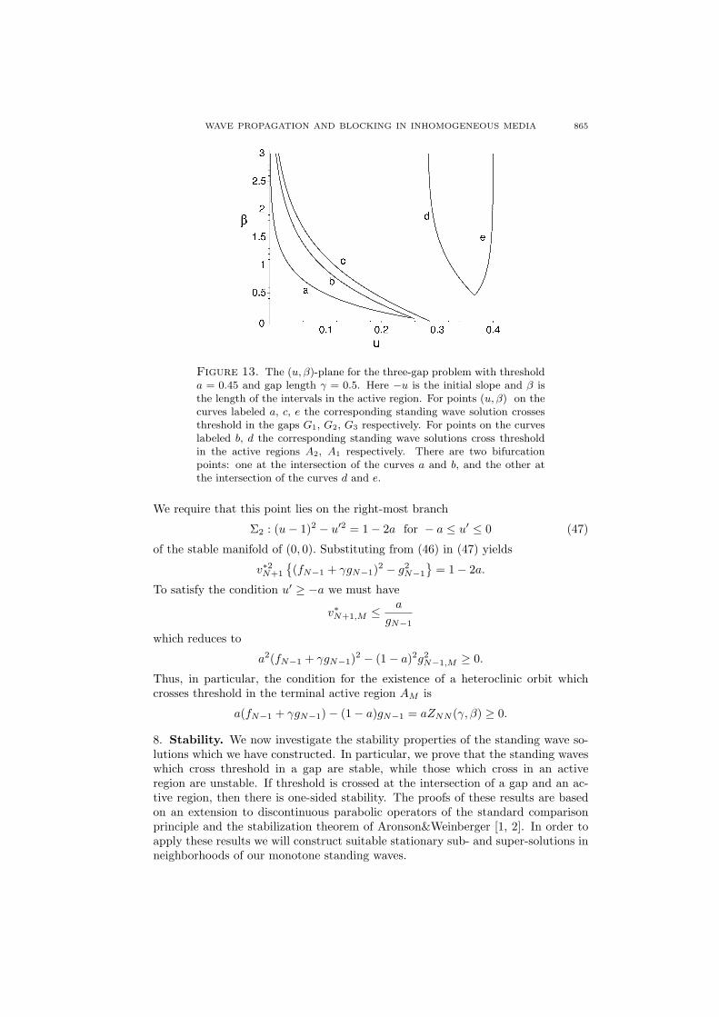
Figure 13. The (u, β)-plane for the three-gap problem with thresholda = 0.45 and gap length γ = 0.5. Here −u is the initial slope and β isthe length of the intervals in the active region. For points (u, β) on thecurves labeled a, c, e the corresponding standing wave solution crossesthreshold in the gaps G1, G2, G3 respectively. For points on the curveslabeled b, d the corresponding standing wave solutions cross thresholdin the active regions A2, A1 respectively. There are two bifurcationpoints: one at the intersection of the curves a and b, and the other atthe intersection of the curves d and e.
We require that this point lies on the right-most branch
Σ2 : (u− 1)2 − u′2 = 1− 2a for − a ≤ u′ ≤ 0 (47)
of the stable manifold of (0, 0). Substituting from (46) in (47) yields
v∗2N+1
{(fN−1 + γgN−1)2 − g2
N−1
}= 1− 2a.
To satisfy the condition u′ ≥ −a we must have
v∗N+1,M ≤ a
gN−1
which reduces to
a2(fN−1 + γgN−1)2 − (1− a)2g2N−1,M ≥ 0.
Thus, in particular, the condition for the existence of a heteroclinic orbit whichcrosses threshold in the terminal active region AM is
a(fN−1 + γgN−1)− (1− a)gN−1 = aZNN (γ, β) ≥ 0.
8. Stability. We now investigate the stability properties of the standing wave so-lutions which we have constructed. In particular, we prove that the standing waveswhich cross threshold in a gap are stable, while those which cross in an activeregion are unstable. If threshold is crossed at the intersection of a gap and an ac-tive region, then there is one-sided stability. The proofs of these results are basedon an extension to discontinuous parabolic operators of the standard comparisonprinciple and the stabilization theorem of Aronson&Weinberger [1, 2]. In order toapply these results we will construct suitable stationary sub- and super-solutions inneighborhoods of our monotone standing waves.

866 D.G. ARONSON, N.V. MANTZARIS AND HANS OTHMER
We are concerned with the parabolic differential operator
Nu ≡ ut − uxx − I(x) {H(u− a)− u} ,
where I(x) is the indicator function on the union of the active regions. N is discon-tinuous at the intersections of the active and passive regions as well as on any curvex = c(t) where u(c(t), t) = a. We will assume, in general, that N is discontinuouson a finite collection of curves C ={c1(t), ..., cm(t)} which are nowhere horizontal.
Comparison Theorem. Let ϕ(x, t) = u(x, t) − v(x, t), where u and v areC2,1((R\C)×R+) ∩ C(R×R+) functions. If
Nϕ ≤ 0 in (R\C)×R+
ϕ(·, 0) ≤ 0 in R
ϕx(cj(t)−, t) ≤ ϕx(cj(t)+, t) for j = 1, ..., m and t ∈ R+.
thenϕ(x, t) ≤ 0 throughout R×R+.
An important consequence of the Comparison Theorem concerns the behavior ofsolutions to the transient problem when the initial datum is a stationary sub- orsuper-solution. A function U is said to be a sub-solution for N if
NU ≤ 0 in (R\C)×R+ (48)
Ux(cj(t)−, t) ≤ Ux(cj(t)+, t) for j = 1, ...,m and t ∈ R+,
and U is said to be a super-solution forN if (48) holds with the inequalities reversed.If U is a sub-solution and v is a solution with U(·, 0) ≤ v(·, 0) then, according to theComparison Theorem, U(x, t) ≤ v(x, t) everywhere. Moreover, we have the nexttheorem.
Convergence Theorem. Let U(x) be a time-independent sub-solution (super-solution) for N and let u(x, t; U) be the solution of the transient problem
Nu = 0 in (R\C)×R+
u(·, 0) = U in R.
Then u(x, t;U) is a nondecreasing (nonincreasing) function of t which for t → ∞approaches the smallest (largest) steady state solution U∗(x) of Nu = 0 such that
U∗(x) ≥ (≤)U(x) for all x ∈ R.
Proofs of these results are essentially given by Pauwelussen [12]. In order toapply these results we prove the existence of suitable sub- and super-solutions inthe neighborhood of each standing wave solution. In particular, we show that astanding wave solution which crosses threshold in a gap is stable since there existsub-solutions below and super-solutions above it. For a standing wave solutionW (x) which crosses threshold in an active region the situation is more complicatedsince the transition from super- to sub-threshold reverses relative positions. Thusthe sub- and super-solutions which we construct straddle the standing wave ratherthan being strictly above or below it. Suppose W crosses threshold in the M th activeregion. We construct steady super-solutions W+ and sub-solutions W− arbitrarilyclose to W which satisfy W+ < W < W−on (0, xM ). By the Convergence Theoremu(x, t;W+) (u(x, t;W−)) converges to the largest (smallest) steady state solutionS satisfying S < W (S > W ). Thus W is unstable.

WAVE PROPAGATION AND BLOCKING IN INHOMOGENEOUS MEDIA 867
Moreover, if we consider a transient problem whose initial datum lies betweentwo standing waves, one crossing threshold in AM−1 and the other crossing in AM ,then it follows from the Comparison Theorem and the Convergence Theorm thatthe solution to that problem will evolve in time to a standing wave which crossesthreshold in GM . This is illustrated in Figure 14.
Figure 14. (a) The three standing wave solutions corresponding to thetwo-gap case (a = 0.2, β = γ = 5.). Solid, dashed and dotted lines rep-resent the standing wave for which the solution crosses threshold withinthe first gap, the first active region, and the second gap, respectively.(b) Transient simulation for initial condition: u0(x) = usw(x)+ ε, whereusw(x) is the standing wave for which the solution drops below thresholdwithin the first active region in (a) and ε = −0.01. The final distribu-tion is shown in a dotted line and is identical to the constructed standingwave shown in (a).
The standing wave which crosses threshold in the M th gap for a specific (γ, β) isgiven by (16), where u∗MN is the initial speed determined by the condition that theendpoint of the phase curve for the standing wave lies on the stable manifold Σ1. Ifwe omit this condition and write (16) for arbitrary values of u, then it is clear thatboth u(x) and u′(x) decreases as u increases. If u1 < u∗MN < u2, let
UN−1(uj) =(
Uj
U ′j
)and UN−1(u∗MN ) =
(U∗U′∗
)
then
U1 > U∗ > U2,
U ′1 > U ′
∗ > U ′2
andq1 > 0 > q2,
where qj = Uj + U ′j with U∗ + U ′
∗ = 0 by construction. It follows that the phasepoint (U1, U
′1) lies above Σ1 while the point (U2, U
′2) lies below it, as shown in Figure
15. We construct a sub-solution below the standing wave by introducing an upwardjump in the derivative at x = yN−1 by setting
U ′2(yN−1+) = −U2 > U ′
2(yN−1−).

868 D.G. ARONSON, N.V. MANTZARIS AND HANS OTHMER
Similarly, we construct a super-solution above the standing wave by introducing a
O P
Σ
Σ
2
3
W
Σ Γ
Γ
11
3
a
−a
W
W
1
2
−u
−u−u
1
2*
Figure 15. Construction of sub- and super- solutions close to a stand-ing wave W which crosses threshold in the gap G2 in the two-gap prob-lem. W1 is a super-solution which lies above W and W2 is a sub-solutionthat lies below W .
downward jump in derivative at x = yN−1 by setting
U ′1(yN−1+) = −U1 < U ′
1(yN−1−).
Suppose now that threshold is reached in the M th active region AM at y = xM+δ,where δ ∈ (0, β). Then
(a
u′(y)
)= ε1 − uA(δ)P (AP )M−1ε
and δ = δ(u) is determined by
a = 1− uεT1 A(δ)P (AP )M−1ε.
Differentiating with respect to u and using the fact that
d
dδA(δ) =
(0 11 0
)A(δ)
yieldsdδ
du= − εT
1 A(δ)P (AP )M−1ε
uεT2 A(δ)P (AP )M−1ε
< 0. (49)
Set b(u) = u′(xM + δ(u)). Then
b(u) = −uεT2 A(δ)P (AP )M−1ε
anddb
du= −εT
2 A(δ)P (AP )M−1ε− udδ
duεT1 A(δ)P (AP )M−1ε.
In view of (49) this becomes
db
du=
{εT1 A(δ)P (AP )M−1ε
}2 − {εT2 A(δ)P (AP )M−1ε
}2
εT2 A(δ)P (AP )M−1ε
.
The sign of db/du is determined by the sign of
(εT1 − εT
2 )A(δ)P (AP )M−1ε= (cosh(β)− sinh(β))(fM−1 − gM−1 + γgM−1).
WAVE PROPAGATION AND BLOCKING IN INHOMOGENEOUS MEDIA 869
Thereforedb
du> 0. (50)
To complete the traversal of AM we apply A(β − δ) to obtain(
vM (u)v′M (u)
)= A(β − δ(u))
(a
b(u)
)
Suppose 0 < u1 < u∗ = v∗MN < u2. Then(
vM (u1)v′M (u1)
)=
(a cosh(β − δ(u1)) + b(u1) sinh(β − δ(u1))a sinh(β − δ(u1)) + b(u1) cosh(β − δ(u1))
)
and by Taylor’s expansion(vM (u1)v′M (u1)
)=
(vM (u∗)v′M (u∗)
)+ (u∗ − u1)R + · · ·,
where
R =(
δ′(u∗){a sinh(β − δ(u∗)) + b(u∗) cosh(β − δ(u∗))} − b′(u∗) sinh(β − δ(u∗))δ′(u∗){a cosh(β − δ(u∗)) + b(u∗) sinh(β − δ(u∗))} − b′(u∗) cosh(β − δ(u∗))
).
In view of (49) and (50), both components of R are negative, so that
vM (u1) < vM (u∗) and v′M (u1) < v′M (u∗) (51)
for sufficiently large u1 < u∗. Similarly
vM (u2) > vM (u∗) and v′M (u2) > v′M (u∗) (52)
for sufficiently small u2 > u∗.At the end of the last gap GN we have
UN−1(u) =(
uN−1(u)u′N−1(u)
)= P (AP )N−M−1
(vM (u)v′M (u)
).
The elements of the matrix P (AP )N−M−1 are all strictly positive and independentof u. Therefore it follows from (51 and (52) that
uN−1(u1) < uN−1(u∗) and u′N−1(u1) < u′N−1(u∗)
anduN−1(u2) > uN−1(u∗) and u′N−1(u2) > u′N−1(u∗).
Moreoverq(u1) < q(u∗) = 0 < q(u2).
Thus the phase point UN−1(u1) is in the fourth quadrant below Σ1 and the phasepoint UN−1(u2) is in the fourth quadrant above Σ1 provided that u1 and u2 aresufficiently close to u∗ with u1 < u∗ < u2.
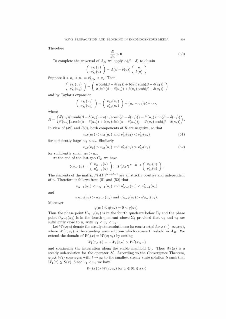
Let W (x; u) denote the steady state solution so far constructed for x ∈ (−∞, xN ),where W (x; u∗) is the standing wave solution which crosses threshold in AM . Weextend the domain of W1(x) = W (x;u1) by setting
W ′1(xN+) = −W1(xN ) > W ′
1(xN−)
and continuing the integration along the stable manifold Σ1. Thus W1(x) is asteady sub-solution for the operator N . According to the Convergence Theorem,u(x.t;W1) converges with t →∞ to the smallest steady state solution S such thatW1(x) ≤ S(x). Since u1 < u∗ we have
W1(x) > W (x; u∗) for x ∈ (0,∈ xM )
870 D.G. ARONSON, N.V. MANTZARIS AND HANS OTHMER
and it follows thatW (x;u∗) < S(x) for all x.
In a similar manner if we extend W2 by setting
W ′2(xN+) = −W2(xN ) < W ′
2(xN−)
then W2(x) is a steady super-solution, and u(x, t;W2) converges down as t →∞ tothe largest steady state solution T (x) such that
W (x; u∗) > T (x) for all x
(cf. Figure 16).
O P
Σ
Σ
2
3
+
Γ
Γ
1
3
W
Σ1
a
−u
−u−u
1
2
*
−a
W
W
1
2
Figure 16. Construction of sub- and super- solutions close to a stand-ing wave W which crosses threshold in the active region A1 in the two-gap problem. W1 is a sub-solution which lies partially above W and W2
is a super-solution which lies partially below W .
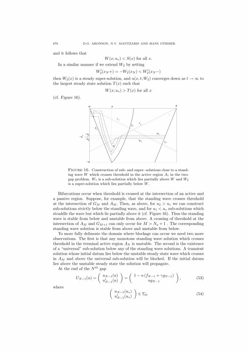
Bifurcations occur when threshold is crossed at the intersection of an active anda passive region. Suppose, for example, that the standing wave crosses thresholdat the intersection of GM and AM . Then, as above, for u2 > u∗ we can constructsub-solutions strictly below the standing wave, and for u1 < u∗ sub-solutions whichstraddle the wave but which lie partially above it (cf. Figure 16). Thus the standingwave is stable from below and unstable from above. A crossing of threshold at theintersection of AM and GM+1 can only occur for M > Na + 1 . The correspondingstanding wave solution is stable from above and unstable from below.
To more fully delineate the domain where blockage can occur we need two moreobservations. The first is that any monotone standing wave solution which crossesthreshold in the terminal active region AN is unstable. The second is the existenceof a “universal” sub-solution below any of the standing wave solutions. A transientsolution whose initial datum lies below the unstable steady state wave which crossesin AM and above the universal sub-solution will be blocked. If the initial datumlies above the unstable steady state the solution will propagate.
At the end of the N th gap
UN−1(u) =(
uN−1(u)u′N−1(u)
)=
(1− u (fN−1 + γgN−1)
ugN−1
), (53)
where (uN−1(u∗)u′N−1(u∗)
)∈ Σ2. (54)

WAVE PROPAGATION AND BLOCKING IN INHOMOGENEOUS MEDIA 871
If u1 < u∗ < u2 then
uN−1(u1) > uN−1(u∗) > uN−1(u2) and u′N−1(u1) > u′N−1(u∗) > u′N−1(u2). (55)
Letq(w) ≡ (1− uN−1(w))2 − u′2N−1(w),
where, in view of (54), q(u∗) = 1− 2a and, in view of (53),
q(u) = u2{
(fN−1 + γgN−1)2 − g2
N−1
}.
Note that
(fN−1 + γgN−1)2 − g2
N−1 = (fN−1 + γgN−1 + gN−1) (fN−1 − gN−1 + γgN−1) > 0.
Therefore q(u) is a strictly increasing function and
q(u1) < q(u∗) = 1− 2a < q(u2).
Since q(u1) < 1 − 2a the phase point UN−1(u1) lies between Σ2 and Σ3. Weconstruct a sub-solution by setting
u′N−1(u1) |xN+ = −√{(1− uN−1(u1))2 − 1 + 2a} > u′N−1(u1) |xN− .
In view of (55) this sub-solution lies above the standing wave. In a similar mannerwe can construct super-solutions below the standing wave. An example is shown inFigure 17. Thus any standing wave solution which crosses threshold in the terminalactive region AN is unstable.
O P
Σ
Σ
2
3
Σ Γ
Γ
11
3W
a
−u
−u−u
1
2
*
−a
WW 12
Figure 17. Construction of sub- and super- solutions close to a stand-ing wave W which crosses threshold in the terminal active region A2 inthe two-gap problem. W1 is a sub-solution which lies above W and W2
is a super-solution which lies below W .
To construct the universal sub-solution we first consider the case γ ≥ 1a− 1.
The locus of endpoints of phase curves in the first passive region is the line u =1 + (1 + γ)u′ which intersects the line u = 0 at or above the level u′ = −a. Thismeans that the phase curve reaches u = 0 before the end of the first gap. Thesub-solution consists of the this phase curve cut off at u = 0 and continued as u ≡ 0
(cf. Figure 18(a)). For γ∗ < γ <1a− 1 the phase curve for the first gap reaches the
level u′ = −a for some u ∈ (0, a). Then integration is then continued into A1 wheredepending on the magnitude of β it may reaches u = 0. If it does we continue it as

872 D.G. ARONSON, N.V. MANTZARIS AND HANS OTHMER
u ≡ 0. If not then we continue into G2 where it must reach u = 0 (cf. Figures 18(b)and 18(c)).
Figure 18. Construction of the “universal” sub-solution for (a) γ ≥1a− 1, (b) and (c) γ∗ < γ < 1
a− 1.
WAVE PROPAGATION AND BLOCKING IN INHOMOGENEOUS MEDIA 873
9. Discussion. We have considered a problem of signal propagation in a non-homogeneous medium. Specifically, we consider the real line partitioned into apassive region P consisting of N open intervals each of length γ, and an activeregion A consisting of N −1 open intervals each of length β separating the intervalsof P together with two semi-infinite intervals surrounding P (cf. Figure 1). Wehave studied the evolution of a quantity u(x, t) that satisfies the diffusion equation
ut = uxx
for x ∈ P and the McKean-Nagumo reaction-diffusion equation
ut = uxx + H(u− a)− u
for x ∈ A. If P = ∅ then, for all but a codimension-1 manifold of initial data,solutions to the initial value problem for the McKean-Nagumo equation approacheither the stable equilibrium u ≡ 0 or u ≡ 1 as t → ∞ [10]. If P 6= ∅ and γ issufficiently small then the situation is similar to the case P = ∅, i.e., most solutionseither die out (tend to 0) or propagate (tend to 1). However for appropriate values ofγ and β in the first quadrant of the (γ, β)-plane (roughly speaking, for γ sufficientlylarge, cf. Figures 6 and 11) there exist stable and unstable standing wave solutionswhich induce a new class of asymptotics, namely, non-trivial stationary patterns.Thus for appropriate initial data the solution to the initial value problem does nottend asymptotically to one of the constant equilibria u ≡ 0 or u ≡ 1, but insteadtends to one of the standing waves. In particular, for the standing waves u → 0 asx →∞ so there is no transmission across the passive region P.
An interesting extension of the present work would be to systems of equationsinvolving a recovery variable, e.g., the system
vt = vxx + I(x) {H(v − a)− v − εw} (56)
wt = I(x)(bv − cw),
where I(x) is the indicator function of the active regions, b and c are positiveconstants, and ε is a non-negative parameter. For ε = 0 the system (56) reducesto the McKean-Nagumo equation, while for ε = 1 and I(x) ≡ 1 the system (56) isthe FitzHugh-Nagumo-McKean system studied by Rinzel & Keller [13] and others.Clearly for ε > 0 the presence of the recovery variable w will facilitate wave block.For ε ¿ 1 one can analyze standing waves and pulses for (56) in the spirit of whatwe have done here for the McKean-Nagumo equation. There is however one majordifference. In the single equation case we were able to use comparison methods toestablish nonlinear stability and instability properties of standing wave solutions.Comparison methods are not, in general, applicable to systems such as (56) sothat one usually has to settle for a linearized stability analysis. Nevertheless weconjecture that the McKean/Moll analysis of the gap-free case can be extendedto the case in which there are gaps for sufficiently small ε. For ε = 1 there arevarious phenomena other than wave-block, e.g., wave reversal [14]. Thus it wouldbe interesting to study the continuation of the solution set to (56) with respect tothe parameter ε.
10. Acknowledgments. NVM and HGO were supported in part by NIH Grant# GM29123, and by the Minnesota Supercomputing Institute. NVM was alsosupported in part by NSF-BES # 0331324.
874 D.G. ARONSON, N.V. MANTZARIS AND HANS OTHMER
11. Appendix. Proof of (28) , (29) and (30). Write
AP =eβ
2R +
e−β
2S,
where
R =
�1 1 + γ1 1 + γ
�and S =
�1 −1 + γ−1 1− γ
�,
and
AP =eβ
2U +
e−β
2V,
where
U =
�1 + γ 1 + γ
1 1
�and V =
�1− γ −1 + γ−1 1
�.
Note that for any positive integer k
Rkε = (2 + γ)k−1Rε = (2 + γ)kε (57)
and
εT Uk = (2 + γ)k−1εT U = (2 + γ)kεT . (58)
Then for M ≥ 2
(AP )M−1ε =e(M−1)β
2M−1(2 + γ)M−1ε +
e(M−3)β
2M−1BM−1ε + · · ·,
where
BM−1 =
M−2Xj=0
RM−2−jSRj ,
and for M ≤ N − 1
εT (PA)N−M =e(N−M)β
2N−MεT (2 + γ)N−M +
e(N−M−2)β
2M−1εT DN−M + · · ·,
where
DN−M =
N−M−1Xj=0
UN−M−1−jV U j .
If M = 1 then B0 = 0 and D0 = 0 when M = N.
Since �fk(γ, β)gk(γ, β)
�= (AP )kε ∼ (2 + γ)k
�eβ
2
�k
ε as β →∞.
it follows that
XMN = (1
a− 1)gM−1(fN−M + γgN−M )− fM−1gN−M
∼ (2 + γ)N−1
�γ∗ + γ(
1
a− 1)
�e(N−1)β
2N−1as β →∞.
Thus (28) holds.To prove (29) we note that in view of (11) and (13) we can write (21) in the form.
ZMN = εT (PA)N−MQ(AP )M−1ε,
where
Q =
1 γ
0 1− 1
a
!.
WAVE PROPAGATION AND BLOCKING IN INHOMOGENEOUS MEDIA 875
Hence
ZMN =e(N−1)β
2N−1(2 + γ)N−1εT Qε
+e(N−3)β
2N−1{(2 + γ)N−MδεT QBM−1ε + (2 + γ)M−1εT DN−MQε}+ · · ·
SinceεT Qε = γ − γ∗
we conclude that
ZMN ∼ e(N−1)β
2N−1(2 + γ)N−1(γ − γ∗) as β →∞ for γ 6= γ∗.
For γ = γ∗ and 2 ≤ M ≤ N − 2
ZMN ∼ e(N−3)β
2N−1{(2 + γ∗)N−M εT QBM−1ε + (2 + γ∗)M−1εT DN−MQε}, (59)
with
Q =
1 γ∗
0 1− 1
a
!.
Write
BM−1 = RM−2S + SRM−2 +
M−3Xj=1
RM−2−jSRj .
Then, in view of (57), we obtain
BM−1ε = (M − 2)(2 + γ∗)M−3RSε+(2 + γ∗)M−2Sε.
NowεT QSε = 2γ∗ and εT QRSε = 0
so that(2 + γ∗)N−M εT QBM−1ε = 2γ∗(2 + γ∗)N−2. (60)
An analogous computation using (58) yields
(2 + γ∗)M−1εT DN−MQε = −2γ∗(1
a− 1)(2 + γ∗)N−2. (61)
Therefore we obtain (30) after substituting (60) and (61) into (59), and recalling thatB0 = D0 = 0.
REFERENCES
[1] D. G. Aronson and H. F. Weinberger, Nonlinear diffusion in population genetics, combus-tion and nerve propagation, in Lecture Notes in Mathematics, Springer-Verlag, Berlin, 446,(1975), pp. 5–49.
[2] , Multidimensional nonlinear diffusions arising in population genetics, Adv. Math., 29(1978), pp. 33–76.
[3] S. Boitano, E. R. Dirksen, and M. J. Sanderson, Intercellular propagation of calciumwaves mediated by inositol trisphosphate, Science, 258 (1992), pp. 292–295.
[4] A. C. Charles, C. C. G. Naus, D. Zhu, G. M. Kidder, E. R. Dirksen, and M. J. Sander-son, Intercellular calcium signalling via gap junctions in glioma cells, J. Cell Biol., 118 (1992),pp. 195–201.
[5] M. O. Enkvist and K. D. McCarthy, Activation of protein kinase C blocks astroglial gapjunction communication and inhibits the spread of calcium waves, J. Neurochem., 59 (1992),pp. 519–526.
[6] T. D. Hassinger, P. B. Guthrie, P. B. Atkinson, M. V. L. Bennett, and S. B. Kater,An extracellular signaling component in propagation of astrocytic calcium waves, Proc. Nat.Acad. Sci., 93 (1996), pp. 13268–13273.
[7] T. J. Lewis and J. P. Keener, Wave-block in excitable media due to regions of depressedexcitability, SIAM J. Appld. Math., 61 (2000), pp. 293–316.
[8] H. McKean, Nagumo’s equation, Adv. Math., 4 (1970), pp. 209–223.
876 D.G. ARONSON, N.V. MANTZARIS AND HANS OTHMER
[9] H. P. McKean, Stabilization of solutions of a caricature of the Fitzhugh-Nagumo equation(2), Comm. Pure & Appld. Math., 37 (1984), pp. 299–301.
[10] H. P. McKean and V. Moll, Stabilization to the standing wave in a simple caricature ofthe nerve equation, Comm. Pure & Appld. Math., 39 (1986), pp. 485–529.
[11] H. G. Othmer, A continuum model for coupled cells, J. Math. Biol., 17 (1983), pp. 351–369.[12] J. P. Pauwelussen, Nerve impulse propagation in a Branching nerve system: A simple
model, Physica, 4D (1981), pp. 67–88.[13] J. Rinzel and J. B. Keller, Travelling wave solutions of a nerve conduction equation,
Biophys. J., 13 (1973), pp. 1313–1337.[14] J. Rinzel and D. Terman, Propagation phenomena in a bistable reaction-diffusion system,
SIAM J. Appld. Math., 42 (1982), pp. 1111–1137.[15] J. Sneyd and J. Sherratt, On the propagation of calcium waves in an inhomogeneous
medium, SIAM J. Appl. Math., 57 (1997), pp. 73–94.[16] J. Sneyd, M. Wilkins, A. Strahonja, and M. J. Sanderson, Calcium waves and oscilla-
tions driven by an intercellular gradient of inositol (1,4,5)-trisphosphate, Biophys. Chem., 72(1998), pp. 101–109.
[17] P. A. Spiro and H. G. Othmer, The effect of heterogeneously-distributed ryR channels oncalcium dynamics in cardiac myocytes, Bull. Math. Biol, 61 (1999), pp. 651–681.
[18] A. Verkhratsky, R. K. Orkand, and H. Kettermann, Glial calcium: homeostasis andsignaling function., Physiol. Rev., 78 (1998), pp. 99–141.
[19] S. Yagodin, L. A. Holtzclaw, and J. T. Russell, Subcellular calcium oscillators andcalcium influx support agonist-induced calcium waves in cultured astrocytes, Mol. and Cell.Biochem., 149 (1995), pp. 137–144.
[20] S. V. Yagodin, L. Holtzclaw, C. A. Sheppard, and J. T. Russell, Nonlinear propagationof agonist-induced cytoplasmic calcium waves in single astrocytes, J. Neurobiol., 25 (1994),pp. 265–280.
[21] J. Yang, S. Kalliadasis, J. H. Merkin, and S. K. Scott, Wave propagation in spatiallydistributed exciable media, SIAM J. Appl. Math, 63 (2002), pp. 485–509.
Received November 2004; revised April 2005.
E-mail address: [email protected]
E-mail address: [email protected]
E-mail address: [email protected]