WAVE GENERATION AND ANALYSIS IN THE LABORATORY WAVE ...
92
WAVE GENERATION AND ANALYSIS IN THE LABORATORY WAVE CHANNEL TO CONDUCT EXPERIMENTS ON THE NUMERICALLY MODELED SPAR TYPE FLOATING WIND TURBINE A Thesis Submitted to the Graduate School of Engineering and Sciences of İzmir Institute of Technology in Partial Fulfillment of the Requirements for the Degree of MASTER OF SCIENCE in Civil Engineering by Kadir AKTAŞ December 2020 İZMİR
Transcript of WAVE GENERATION AND ANALYSIS IN THE LABORATORY WAVE ...

WAVE GENERATION AND ANALYSIS IN THE
LABORATORY WAVE CHANNEL TO CONDUCT
EXPERIMENTS ON THE NUMERICALLY
MODELED SPAR TYPE FLOATING WIND
TURBINE
A Thesis Submitted to
the Graduate School of Engineering and Sciences of
İzmir Institute of Technology
in Partial Fulfillment of the Requirements for the Degree of
MASTER OF SCIENCE
in Civil Engineering
by
Kadir AKTAŞ
December 2020
İZMİR

ACKNOWLEDGMENTS
I would like to express my deepest gratitude to my dear advisor Assoc. Prof. Dr.
Bergüzar Özbahçeci for the guidance and support she provided through my M.Sc. study.
This thesis is written thanks to her being the most patient mentor a student can ask for.
imparting her knowledge and expertise in this study. Also, I thank her for providing
opportunities such as sharing some findings of this work at the national conference “9.
Kıyı Mühendisliği Sempozyumu” held in Adana, November 2018.
Besides my advisor, I would like to thank Assoc. Prof. Dr. Ünver Özkol for
allowing me to work on this astonishing project and become a part of this great team.
This study was funded by the Scientific and Technological Research Council of
Turkey, TUBITAK under 217M451.
I would like to send my sincere gratitude to my colleague Ruwad Adnan Al
Karem who provided the design for the spar platform model.
Also, I would like to thank Bahadır Öztürk for opening up his house whenever I
had to stay late studying, and to thank Hazal Emet and Cemal Kılıç for the help they
provided in the laboratory.
I would like to thank my father, Mehmet Aktaş, for teaching me perseverance.
Lastly, I would like to thank my mother, Gülnur Ölçer, who passed the passion
for knowledge down to her son.

To my wife, Emel Aktaş

iv
ABSTRACT
WAVE GENERATION AND ANALYSIS IN THE LABORATORY
WAVE CHANNEL TO CONDUCT EXPERIMENTS ON THE
NUMERICALLY MODELED SPAR TYPE FLOATING WIND
TURBINE
The oceans offer immense potential for harvesting sustainable wind energy, with
stronger and steadier winds for locations further offshore. Since the feasibility of fixed-
bottom offshore wind turbines decreases with increasing water depth, floating offshore
wind turbines (FOWT) becomes a promising field of study.
As part of a TÜBİTAK project (217M451) that investigates the dynamic
performance of different FOWT designs under wind and wave loads, the necessary
laboratory wave generation, analysis, and test set-up to conduct physical model
experiments of a spar-type FOWT model is established in this study. An investigation
of the wavemaker theory yielded that using first-order wavemaker solutions in the
laboratory leads to the generation of spurious harmonic waves that do not appear in
natural waves. Therefore, the second-order solutions are applied to the piston-type wave
generator for a closer approximation of natural waves in laboratory conditions.
A numerical model investigation of a reference spar-type FOWT is conducted
to gain insights into spar design using ANSYS AQWA. The results indicate that the
spar model dynamic responses are susceptible to low-frequency waves in pitch and
surge degrees of freedom as its natural frequency lies in that region which further
emphasizes the importance of generating laboratory waves using second-order
wavemaker theory. Additionally, a spar-type floating platform is modeled at the 1/40
Froude scale, to use in the hydraulic model experiments. The wave measurement set-up
is fully implemented and theoretically generated waves are measured for validation. In
conclusion, regular and irregular wave generation and wave analysis in the time and the
frequency domain could be possible in the wave channel of IZTECH Civil Engineering
Hydraulic Laboratory.

v
ÖZET
SAYISAL OLARAK MODELLENEN SPAR TİPİ YÜZER RÜZGAR
TÜRBİNİNİN FİZİKSEL MODEL DENEYLERİ İÇİN
LABORATUVARDA DALGA ÜRETİMİ VE ANALİZİ
Açık denizler karaya kıyasla daha yüksek ve sürekli rüzgar profilleri göstermesi ile
sürdürebilir rüzgar enerjisi sektöründe yükselişini sürdürmektedir. Sabit tabanlı açık
deniz rüzgar türbinlerinin enerji potansiyelinin daha yüksek olduğu karadan uzak ve
derin bölgelerde elverişsiz olması ile yüzer rüzgar türbinlerinin önemi artmaktadır.
Bu çalışmada 217M451 kodlu TÜBİTAK projesi kapsamında sayısal modellemesi
yapılmış spar tipi bir yüzer rüzgar türbinin fiziksel deneylerini gerçekleştirmek
amacıyla İYTE Hidrolik Laboratuvarındaki dalga kanalına yerleştirilmiş piston tipi
dalga üretecinin doğradaki düzensiz dalgalara benzer dalga serileri üretmesi
sağlanmıştır. Teorik bir spektruma uygun rastgele dalga zaman serileri oluşturulup bu
dalgaları laboratuvar dalga kanalında elde etmek için gereken zamana bağlı dalga pedalı
konumları ikinci mertebe transfer fonksyonları ile hesaplanmış, pedal hareketiyle
oluşturulan dalgalar kanala yerleştirilen dalga ölçerler yardımıyla okunmuştur.
Oluşturulan teorik dalgalar matematiksel analiz yöntemleri ile ve dalga üretecinin
ürettiği dalgalar laboratouvar ölçümleri ile doğrulanmıştır.
Ayrıca spar tipi bir platformun ANSYS AQWA programında nümerik
modellenmesi yapılmış, düşük frekanslı dalgaların platform tepkilerine yüksek ölçüde
etkisi olduğu gözlemlenmiştir. Proje kapsamında incelenecek olan spar tipi yüzer rüzgar
türbinin platformu, 1:40 Froude ölçeği kullanarak modellenmiş ve imal edilmiştir.
Sonuç olarak İYTE Hidrolik Laboratuvarı dalga kanalında ikinci dereceden düzenli ve
düzensiz dalgalar üretilmiş, kullanılan metodlar doğrulanmış ve fiziksel model
deneyleri için gerekli hazırlıklar tamamlanmıştır.

vi
TABLE OF CONTENTS
ACKNOWLEDGMENTS................................................................................................ii
ABSTRACT.....................................................................................................................iv
ÖZET.................................................................................................................................v
LIST OF FIGURES........................................................................................................viii
LIST OF TABLES.............................................................................................................x
INTRODUCTION ............................................................................................................ 1
1.1. Research Setting & Background ............................................................. 1
1.2. Aim and Scope of the Study ................................................................... 3
1.3. The Structure of the Thesis ..................................................................... 5
LITERATURE REVIEW ................................................................................................. 6
2.1. Wavemakers ............................................................................................ 6
2.2. Synthesis of Random Waves ................................................................ 10
HYDRODYNAMIC MODELING OF THE SPAR-TYPE PLATFORM FOR A
FLOATING OFFSHORE WIND TURBINE ......................................... 13
3.1. An Overview on Numerical Model and OC3 Offshore Code
Comparison Study ................................................................................. 13
3.2. Modeling of a Spar-Type Floating Platform ......................................... 15
3.2.1. Static Equilibrium ............................................................................ 17
3.2.2. Natural Frequencies ......................................................................... 18
3.2.3. Free Decay Tests .............................................................................. 19
3.2.4. Hydrodynamic Response with Regular Waves ................................ 20
3.2.5. Hydrodynamic Response with Irregular Waves .............................. 22
WAVE GENERATION AND ANALYSIS IN THE LABORATORY ......................... 24
4.1. Wave Environment ............................................................................... 24

vii
4.1.1. Regular Waves ................................................................................. 24
4.1.2. Irregular Waves ................................................................................ 26
4.2. Analysis Procedures of Wave Datasets ................................................ 27
4.2.1. Frequency Domain Analysis ........................................................... 28
4.2.2. Spectral moments ............................................................................. 30
4.2.3. Time Domain Analysis .................................................................... 31
4.3. Preparation of the Wave Generator Signal ........................................... 32
4.3.1. Synthesis of the Irregular Wave Series ............................................ 33
4.3.2. Wave Board Displacement Functions by Wavemaker Theory ........ 37
4.4. Reflection Analysis ............................................................................... 52
LABORATORY SETUP FOR PHYSICAL MODEL EXPERIMENTS OF THE SPAR-
TYPE FLOATING OFFSHORE WIND TURBINE .............................. 57
5.1. Wave Flume Setup ................................................................................ 57
5.2. Model set-up ......................................................................................... 60
5.3. Wave Measurement and Analysis ......................................................... 67
5.3.1. Calibration & Measurement ............................................................. 69
5.4. Passive Absorption of the Reflected Waves ......................................... 71
CONCLUSIONS ............................................................................................................ 74
REFERENCES ............................................................................................................... 77

viii
LIST OF FIGURES
Figure Page
Figure 1.1: Three different FOWT concepts .................................................................... 2
Figure 1.2: The six degrees of freedom of rotations and translations ............................... 4
Figure 2.1: A sketch of piston (left), flap (middle), and plunger (right) wavemakers ... 10
Figure 3.1: Spar-type FOWT modeled in AQWA® ........................................................ 16
Figure 3.2: LC 1.2, Comparison of the natural frequencies in six DOFs ....................... 18
Figure 3.3: LC 1.4 free decay test results in surge, heave, pitch (AQWA) .................... 19
Figure 3.4: LC 1.4 free decay test results in the surge, heave, pitch (OC3) ................... 20
Figure 3.5: LC 4.1 time-domain response analysis results for AQWA model ............... 21
Figure 3.6:: LC 4.1 time-domain response analysis results for OC3 participants .......... 21
Figure 3.7: LC 4.2 frequency domain response analysis results for AQWA model ...... 22
Figure 3.8: LC 4.2 frequency domain response analysis results for OC3 participants ... 23
Figure 4.1: Regular wave ................................................................................................ 25
Figure 4.2: A comparison of PM and JONSWAP spectrum with the same wave
parameters (Hs=1.5m, Ts=7.6s) ...................................................................................... 27
Figure 4.3: Time series (left) and spectra (right) of a bichromatic wave (up) and an
irregular wave (down) ..................................................................................................... 30
Figure 4.4: Flow chart describing the steps involving wave generation ........................ 33
Figure 4.5: Randomly generated irregular wave series .................................................. 35
Figure 4.6: Comparison of the theoretical spectrum obtained by Eq.(4.4)(left), and the
one obtained from the synthesized irregular waves (right) ............................................. 36
Figure 4.7: a 2-D sketch of the generalized wave generator system .............................. 37
Figure 4.8: Wave height to stroke ratio for the piston-type wavemaker ........................ 42
Figure 4.9: Second-order wave board displacement for a regular wave ........................ 44
Figure 4.10: Spectra of the targeted irregular wave and the necessary wave board
motion to generate it ....................................................................................................... 47
Figure 4.11: An irregular wave series and the corresponding first-order wave board
displacement time series ................................................................................................. 48
Figure 4.12: Comparison of transfer functions for progressive wave and evanescent
modes .............................................................................................................................. 49

ix
Figure Page
Figure 4.13: real (upper) and imaginary (lower) components of 𝐹 ± transfer function for
subharmonic (left) and superharmonic (right) corrections ............................................. 51
Figure 4.14: real (upper) and imaginary (lower) components of 𝐹 ± transfer function for
subharmonic (left) and superharmonic (right) corrections ............................................. 51
Figure 4.15: System definition for reflection analysis .................................................... 53
Figure 4.16: Spectral resolution in the effective range of frequencies ........................... 56
Figure 5.1: Laboratory wave flume ................................................................................ 57
Figure 5.2: Side view of the piston-type wave generator ............................................... 58
Figure 5.3: Top view of the piston-type wave generator showing the servo motor and
ball screw shaft ............................................................................................................... 59
Figure 5.4: Wind nozzle and connected fans .................................................................. 59
Figure 5.5: Scaled model of the spar-type floating platform with one mooring chain
attached ........................................................................................................................... 63
Figure 5.6: Dimensions of the scale model of the spar-type floating platform .............. 64
Figure 5.7: Pulley system for the leeward mooring lines ............................................... 65
Figure 5.8: Top-view sketch of the wave flume ............................................................. 66
Figure 5.9: Wave probes, mounted on the wave flume .................................................. 68
Figure 5.10: Wave gauge monitor .................................................................................. 68
Figure 5.11: Linear regression to obtain the depth-voltage relationship ........................ 70
Figure 5.12: Irregular wave measurement taken in the wave flume ............................... 71
Figure 5.13: Dissipating beach ....................................................................................... 72
Figure 5.14: The wave absorbing steel cage ................................................................... 73

x
LIST OF TABLES
Table Page
Table 3.1: Overview of participants’ models .................................................................. 14
Table 3.2: OC3 load-case simulations ............................................................................ 15
Table 3.3: Properties of the spar platform ...................................................................... 17
Table 3.4: LC 1.3, Static equilibrium results .................................................................. 18
Table 3.5: AQWA model natural frequencies (Hz) ........................................................ 18
Table 4.1: Validation of the wave generation scheme with spectral and statistical
parameters ....................................................................................................................... 36
Table 5.1: Froude scale factors for the laboratory experiments ..................................... 61
Table 5.2: Floating offshore wind turbine properties ..................................................... 61
Table 5.3: Mooring system properties ............................................................................ 62
Table 5.4: Wave probe calibration example ................................................................... 69

1
CHAPTER 1
INTRODUCTION
1.1. Research Setting & Background
Wind energy is a much sought-after form of sustainable, clean energy due to its low
impact on the environment, low emission of carbon and other harmful substances, and
due to it not relying on fuel and freshwater. The global installed capacity of wind
energy shows a steady increase for nearly twenty years (GWEC 2019). However, there
is a tendency towards offshore wind energy lately in the market.
The offshore wind energy potential is often associated with stronger and steadier
wind characteristics, which provides the advantages of an increased energy yield and
longer operating life. This effect becomes more and more pronounced for locations
further offshore. Offshore wind turbines with foundations that are fixed to the seabed
are installed in the initial efforts to harvest the offshore wind energy. However, to
benefit more from the energy potential of offshore winds, as well as to avoid
complications such as visually polluting the urban areas or damaging the local fauna
and flora, the investments and the research efforts displayed a shift towards further
offshore and, by extension, deeper waters. Fixed-bottom offshore wind turbines cease
being feasible in deeper waters, which led to the development of floating offshore wind
turbines (FOWT).
A floating offshore wind turbine can be described as a wind turbine mounted on a
floating platform, which can maintain stability and keep stationary under the wind,
wave, and current loads by using any combination of ballast, buoyancy, and taut or
catenary mooring lines. The performance and safety are directly related to the stability
and station-keeping abilities of the FOWT. Several FOWT design concepts gained
prominence in that regard, such as the spar-buoy concept, which mainly uses ballast
weight and high draft, the semi-submersible concept, which mostly takes advantage of a
large water-plane area and ballast weight, and the tension-leg platform (TLP), which
makes use of taut mooring lines that anchor the platform to the seabed, to achieve

2
stability. Figure 1.1 provides the example platform models that use these stabilization
schemes.
Figure 1.1: Three different FOWT concepts
(source: Butterfield et al. 2005)
In tandem with the research efforts on the subject, offshore wind energy investments
soared globally with the cumulative installed capacity tripling between 2010 and 2019,
and a projected increase of another sixfold by 2030. However, to this day, offshore wind
energy remains a small portion of the wind energy industry and there is so much room
for research regarding the design, optimization, and development of floating offshore
wind turbines.
Physical model experiments have a wide-spread use in the research of floating
offshore wind turbines. They provide means to test, calibrate, and validate the
performance and feasibility of a design and are especially useful when complemented
with numerical model studies. Large-scale physical experiments usually require a great
deal of funding and workforce, and a research field such as floating offshore wind
turbines is not an exception. However, a physical system can be represented as a small-

3
scale model, which can demonstrate similar behavior to the prototype under the same
environmental loads. The laws of similitude apply in the scale-model experiments,
which are essential to relate the model and the prototype to each other. The way to
achieve similitude in physical experiments is to keep a dimensionless parameter
constant in the model and the prototype. In the experiments concerning FOWTs, the
main problem is achieving stability, and the main environmental loads acting on the
structure is the wave loads, which are mostly associated with inertial and gravitational
forces, so Froude number is used as the scaling criterion, which gives the ratio of
inertial and gravitational forces. However, a comprehensive physical model of a FOWT
will also require the wind loads to be taken into account, which is best represented with
Reynold's number as the scaling criterion. This discrepancy is usually compensated by
keeping the wind force to wave force (alternatively, wind speed to wave celerity) ratio
constant, as well as maintaining the wind turbine tip speed ratio (TSR) between the
model and the prototype (Martin et al. 2014a).
Wave reproduction in the laboratory wave channel is essential to conduct physical
model experiments. In older times only regular waves that have constant wave height
and period could be produced in the laboratories. However, regular waves do not
represent the real waves that are irregular with different wave height and the period in a
time series in nature. Developments in the wavemaker theory and technology made it
possible to reproduce irregular waves in the laboratory. Yet, there are only a few
laboratories in the world that are capable of irregular wave generation.
1.2. Aim and Scope of the Study
This study aims to provide an appropriate laboratory setup for the physical model
experiments of floating offshore wind turbines including the development of a wave
generator capable of reproducing both regular and irregular waves; wave analysis in the
time and the frequency domain in the laboratory wave flume. The main objectives are as
follows:
1- the numerical investigation of the hydrodynamic behavior of a reference spar-
type FOWT

4
2- the synthesis of irregular wave series that are representative of those
encountered in nature
3- the calculation of the wave board motion that can reproduce the second-order
waves correctly for a piston-type wave generator
4- the production of a physical model of a numerically tested spar-type FOWT
design.
5- the establishment of the laboratory set-up required to conduct physical model
experiments of the FOWT model in the future
6- Wave reflection analysis
The wave flume at IZTECH Hydromechanics Laboratory is used in this study,
which allows the generation of unidirectional waves. It means that the enabled degrees
of freedom (DOFs) for the FOWT will be surge, heave, and pitch in future physical
experiments. Therefore, the same DOFs are investigated in the numerical study given in
chapter 3. The six degrees of freedom for floating structures are shown in Figure 1.2.
Figure 1.2: The six degrees of freedom of rotations and translations
Any efforts involving the generation of the wind and correspondingly, the
production of the upper structure of the FOWT which consists of the tower, hub, and
blades are kept out of scope, as well as the mechanical design of the piston-type wave
generator and the conversion of the calculated wave board motions to the corresponding
electrical signals for the wave generator.

5
1.3. The Structure of the Thesis
The thesis consists of the following chapters; a literature review on the FOWTs,
wavemaker theory, and wave generation in laboratory conditions is given in Chapter 2.
A numerical model study on the hydrodynamic response of a reference spar-type
floating offshore wind turbine under wave loads is conducted and the results are
provided in Chapter 3. The complete wavemaker theory is provided, and the methods to
generate regular and irregular waves correct to the second-order are given in Chapter 4.
The laboratory setup for the physical model tests for FOWTs is described and
validations to the theoretically generated waves are supplied with wave measurements
taken in the wave flume in Chapter 5. The conclusions are drawn from the study, with
the description of the limitations, and the recommendations for the next stages in the
laboratory experiments are provided in Chapter 6.

6
CHAPTER 2
2. LITERATURE REVIEW
Global wind energy harvest is a consistently growing sector (GWEC 2019) and
the oceans offer a vast energy potential. Due to the low surface tension, steadier and
stronger winds are encountered on open seas (Landberg 2016), providing advantages
such as a more efficient energy harvest and longer service life for the wind turbines
(Snyder and Kaiser 2009). For the locations near shore, fixed-bottom offshore wind
turbines are practical, yet, they cease to be feasible for waters deeper than thirty meters.
To access the potentially more profitable open seas, floating offshore wind turbines
should be used. For more than a decade, the potential in offshore wind energy is
realized and the sector is growing rapidly, with a projected increase of another sixfold in
less than a decade (BNEF 2018).
The main research problem in floating offshore wind turbine studies is the
dynamic stability performance of the structure. Physical model experiments offer a
good approach to investigate the stability of the floating offshore wind turbines under
wind and wave loads. Conducting scale model experiments rather than full-scale
prototype experiments is often cheaper and more practical (Chakrabarti 1995). To
approximate natural environmental loads in laboratory conditions, the proper generation
of naturally occurring waves is more than a necessity. Therefore, producing a wave
generator becomes a necessity to conduct physical model experiments.
2.1. Wavemakers
The wavemaker theory is a long-studied subject. Stokes (1880) defined wave
profiles with velocity potentials as parameters of perturbation series, where wave
steepness is chosen as the small ordering parameter. Biesel (1951) defined the first-
order transfer function that gives the relation between the displacement of a piston-type
wave board and the produced waveform. The velocity profile of a fluid flow in nature
can be described with a parabolic function, whereas in the laboratory conditions, the

7
velocity profile of a planar wave board will be uniform. The concept of velocity profile
mismatch and the resulting second-order effects are also pointed out there. Ursell, Dean,
and Yu (1960) made efforts to validate the first-order theory in an experimental setup
for the first time, using a piston-type wave generator in a laboratory wave flume.
Although the accuracy of the results was limited by the reflection in their setup,
conclusive results were achieved nonetheless, with less than four percent experimental
error. Fontanet (1961) developed a second-order approximation for regular waves by
using the Lagrangian approach. He noted the spurious superharmonics generated by the
oscillation of the wave board and proposed to suppress them by adding a second-order
superharmonic component to the first order wavemaker signal. The generation of
spurious harmonic waves in laboratory conditions is of great importance and researchers
have conducted extensive studies tackling this problem and those will be mentioned
later on. Sulisz and Hudspeth (1993) provided an Eulerian theory by presenting
eigenvalue solutions correct to the second order for the fluid motion generated by the
monochromatic sinusiodal motion of a wavemaker.
First-order wavemaker theory, when used in two-dimensional laboratory flumes,
generates additional free waves that are not originally in the control signal. Those waves
are not bound to the wave groups and move freely instead, at their own celerity. That
behavior may sometimes reflect and act to cancel the bound harmonic waves naturally
traveling with the wave group and sometimes may enhance the amplitude of the bound
harmonic waves. Those waves are called “the spurious-free waves” and have to be dealt
with to generate proper time series in the laboratory conditions.
There are three types of spurious waves (Barthel et al. 1983). “Parasitic free
waves” occur due to boundary conditions of the first order wavemaker theory not
meeting the requirements of the second-order bound wave. When the backward
component of the orbital velocity of bound wave troughs comes in contact with the
wave board, it is reflected with the same phase but a smaller, opposite amplitude. The
first-order wavemaker theory boundary condition assumes very small displacements for
the wave board, in reality, however, it makes finite oscillations about its mean position.
That gives rise to the spurious long waves that are conveniently termed as
“displacement free waves”. Finally, “local disturbance-free waves” are generated by
evanescent modes that decay exponentially in the wavemaker theory.

8
It is important to note that in second-order wavemaker theory, waves are often
described in terms of bichromatic waves that consist of the difference or the summation
of each possible interacting frequency pairs that are in the targeted wave spectrum.
These terms are termed as “subharmonic” and “superharmonic”, respectively (Mansard
1988). Subharmonic terms are used to describe long waves and superharmonic terms to
describe second-order higher harmonic effects.
Ottesen-Hansen (1978) defined a method to quantify subharmonic and
superharmonic effects without the assumption of a narrow banded spectrum by deriving
a transfer function in which second-order harmonic contributions are written in terms of
interacting first order components. Flick and Guza (1980) theoretically defined first-
order theory in laboratory conditions that will produce spurious harmonic waves, they
verified this statement with laboratory experiments. Ottesen-Hansen et al. (1980)
investigated spurious long waves when irregular waves are generated using the first-
order wavemaker theory. The study remarked that the longwave energy plays an
important role when the oscillation of moored bodies is of concern to the laboratory
setup. Furthermore, a second-order method for a piston-type wavemaker is derived that,
when superposed with the first-order wave signal, would eliminate the so-called
‘parasitic’ component of long waves. Additionally, an alternative approach is proposed
in the laboratory setup which utilizes shoaling properties of the waves to reduce
parasitic wave influence. A complete method to eliminate spurious subharmonic free
waves is provided in Sand (1982). The method provides means to calculate second-
order compensation signals for each spurious long wave to be added to the first order
wavemaker signal.
In nature, irregular wave trains often have nonlinear aspects due to the higher
harmonic waves that are bound to the wave group. Second-order higher harmonics
alters the wave train in a way that produces steeper wave crests and flatter wave
throughs. First-order wavemaker theory comes short with the generation of nonlinear
features of a wave train. Sand and Mansard (1986) derived a method for laboratory
generation of the higher harmonics while eliminating the spurious superharmonic free
waves.
Later, Schäffer (1996) derived a full second-order wavemaker theory. The
theory includes both subharmonic and superharmonic corrections in the second-order

9
and can be used with both rotational and/or translational wavemaker types. In the
second-order solutions, infinite summation terms related to the evanescent modes
appear. To save computation time, an asymptotic summation method developed by
Schäffer (1994) is utilized. This method is also adopted in this study due to its efficient
computation scheme and complete secondary harmonic correction techniques. The
theory is later extended for multidirectional waves in three-dimensional laboratory
basins (Schäffer and Steenberg 2003).
A different approach was developed by Spinneken and Swan (2009a) to
wavemaker theory. Instead of the usual position-controlled wavemaker approach, they
used force feedback control. The paper reports that force-controlled wavemakers
produce less pronounced second-order spurious waves and it also provides a method to
eliminate the remaining spurious waves. However, the study is limited to the flap-type
wave generators and regular wave cases. Spinneken and Swan (2009b) validate the
force feedback control method with experimental data.
There are several approaches when it comes to the shape of the wavemaker and
the underlying principle of its motion. One of the earliest, perhaps the most common,
types are piston and flap which are planar in shape and they force the waveform by
utilizing their oscillatory motion. The aforementioned scholars Biesel (1951), and
Ursell, Dean, and Yu (1960) both used piston-type wave generators in their experiments
Gilbert, Thompson, and Brewer (1971) provided design curves for piston and flap-type
wave generators, Hughes (1993) gave a good comparison of piston and flap-type wave
generators as the wave height to stroke ratio being a function of wavenumber and depth.
It can be deduced from the comparison that piston wavemakers are more efficient in
regards to the amount of stroke needed to produce the same height of waves. On the
other hand, it was often argued that flap-type wave generators give a closer
representation to the parabolic shape of the natural velocity profile of fluids in deep
water waves and piston-type wave generators give a closer approximation to that of
shallow waters (Dean and Dalrymple 1984) but that velocity mismatch was proved to
cause second-order harmonic effects in every type of wave generators and the problem
of elimination of these spurious effects has been tackled extensively in later studies.
Hyun (1976) analyzed the first-order solution for a wedge type wave board hinged at a
depth above an arbitrary distance from the channel bed, also known as the plunger-type

10
wave generator. The distinctive property of plunger type wavemakers is that instead of
the usual horizontal motions of the wave board, it forces the formation of waves by
vertical motions of a wedge-shaped wave board. The mathematical description of the
waves generated by a plunger-type wavemaker for general shapes in deep water
conditions is given by Wang (1974), describing the generated waves as a function of
plunger period and stroke. Wu (1988) later improved the theory using a semi-analytical
method and also incorporating the effects of the water depth. Since there are many
types of wavemakers a choice can be made considering the research problem, laboratory
conditions, wave cases, and wavemaker theory being used (and cost, if necessary).
Figure 2.1: A sketch of piston (left), flap (middle), and plunger (right) wavemakers
(source: Sand and Donslund 1985)
2.2. Synthesis of Random Waves
To create valid signals for the wavemaker, irregular wave time series must be
generated synthetically. There are a lot of established wave generation schemes but the
most prevalent ones can be classified under those three approaches: Nondeterministic
wave synthesis, deterministic wave synthesis, white noise filtering. The
nondeterministic wave synthesis approach, as the name suggests, uses nondeterministic
phases and amplitudes, therefore the synthesized wave series will not produce the target
spectrum directly (Tuah and Hudspeth 1982). This behavior is analogous to the real
ocean waves. To approach the target spectrum, a large number of synthesized waves
should be averaged (Funke, Mansard, and Dai 1988). A well-known example of this

11
approach is the ‘random complex spectrum method (nondeterministic spectral
amplitude model)’, which uses Fourier coefficients ‘a’ and ‘b’ that are set randomly,
adhering to a Gaussian distribution with zero mean and unit variance. The created
spectrum is then multiplied by the square root of the function of the target spectrum,
then inverse Fourier transform is applied to generate the time series (Miles and Funke
1989).
Deterministic wave synthesis approach models a Gaussian distribution of wave
heights as well as the representation of wave energies by an energy spectrum.
Moreover, this approach makes it possible to acquire the exact target spectrum in the
synthesized waves. One can argue that this is not analogous to the real ocean behavior
but engineers using this type of wave synthesis models have the freedom to have more
control over the properties of generated waves. An example of this approach by Goda
(1970) is named the random phase method (‘deterministic spectral amplitude model’)
where the Fourier components are derived from a target spectrum, using random phases
ranged between 0 to 2π. Random wave time series are synthesized using the inverse
Fourier Transform. An advantage of this method is that if a pseudorandom number
generation algorithm is used in the random phase generation scheme, the same time
series can be generated by remembering the ‘seed’.
The white noise filtering approach makes use of the generation of random
number series (white noise) that have a uniform or Gaussian probability distribution.
An advantage of this approach is that since the pseudorandom number generators’
capacity to generate number sequences that are non-recurring are virtually infinite, the
target spectrum can be approximated as a continuous function rather than a set of finite
discrete frequencies. Samii and Vandiver (1984) provided a method using this approach
where generated white noise sequences are digitally filtered to acquire a time series that
matches their targeted Bretschneider spectrum. Miles and Funke (1988) numerically
investigated seven wave synthesis methods that fall under those three approaches and
concluded that the differences in the mean values and the standard deviations of the
wave parameters are insignificant between those methods. If the number of discrete
frequencies used is sufficient, synthesis methods involving inverse FFT procedures will
be quite realistic as the wave records will be non-recurring. Therefore the researcher is

12
free to choose one of those methods according to their needs in computation time and
convenience.
Another important aspect of creating a random wave series is the assumption of
a wave spectrum. According to the needs of the research, adopted spectra should give a
good representation of the investigated environment. If the problem can be described,
for example, by wind developed waves with the influence of swell generated by remote
storms, a representative frequency spectrum would probably have more than one peak
whereas a single-peaked spectrum can represent conditions where swell becomes
dominated by high, storm waves (Goda, 1999). As the long term wave recordings at
single points proliferated, several models of ocean wave spectra have been developed.
Pierson and Moskowitz (1964) gave the famous Pierson-Moskowitz spectrum for fully
developed oceans at wind speeds observed at 19.5m heights. Using a wide range of
locations for measurement, Bretschneider (1959) developed a spectrum with the
assumption of a linear correlation between wave height and period squared. By
modifying the function factoring in the significant height and period, and their relation
to wave spectrum, Mitsuyasu (1970) reformed the function known as the Bretschneider-
Mitsuyasu spectrum. Due to observations in the program called Joint North Sea Wave
Project spectra of waves where the fetch is limited and the winds are strong show
characteristically sharp peaks. Hasselmann (1973) developed the JONSWAP spectrum
by keeping the dimensionless fetch as the main parameter and introducing a peak
enhancement factor to better achieve a better correlation to the phenomenon. Later,
Goda (1988) expressed the spectrum in terms of the significant wave height and peak
period. Based on the wind-wave coupled simulations at NASA Wallops Flight Center,
Huang et al. (1981) observed that the high-frequency end of the spectrum has, most of
the time, a different slope than proposed in the earlier studies, especially when the
winds are relatively weak. This led to the definition of the model called the Wallops
spectrum, which is later expressed by Goda (1988) in terms of the significant wave
height and peak period. Bouws et al. (1985) proposed the TMA spectrum for finite
depth cases. Their model gives milder slopes in the high-frequency end of the spectrum,
which is better suited to be used in shallow water conditions.

13
CHAPTER 3
3. HYDRODYNAMIC MODELING OF THE SPAR-TYPE
PLATFORM FOR A FLOATING OFFSHORE WIND
TURBINE
3.1. An Overview on Numerical Model and OC3 Offshore Code
Comparison Study
There are several platform types for FOWTs that each adopts a different
approach to achieve stability. The most popular ones include; spar-type platforms, semi-
submersible platforms, and tension-leg platforms (Butterfield et al. 2005). In this study
spar, type floating platform is used since it has applications in the world with known
properties. Before the physical model experiment stage, to investigate the
hydrodynamic behavior of the FOWT with a spar type platform, a numerical model
study is carried out.
The ANSYS™ AQWA® package is used in the numerical modeling, which
allows the user to simulate the motion of the floating structure in the time domain and
provides tools for the investigation of the structural responses in the frequency domain.
For hydrodynamic models, the AQWA package offers potential flow or Morison’s
equation-based applications. Structure response in time and frequency domain is solved
under hydrodynamic forces such as inertia forces, drag forces, Froude-Krylov forces,
and diffraction forces. Typically, two systems used in the analysis of a floating structure
(Aqwa 2013):
1- A hydrodynamic diffraction system is used to calculate hydrostatic analysis
of the structure. The definition of load cases consisting of regular or irregular
waves is possible, which allows the modeling of wave forces for diffracting
structures.
2- A hydrodynamic response system is used, taking the parameters and
solutions in the hydrodynamic diffraction system as input, to obtain dynamic

14
response analysis of the structure in time and/or frequency domain. The
system also allows the definition of mooring line connections and
calculation of the time or frequency domain performance analysis of such
elements.
A spar-type FOWT model is defined in Jonkman (2010) for a numerical code
collaboration study named OC3 with participants from 18 countries and results are
presented in (Jonkman and Musial 2010). Some of the participants’ models and the
theories behind their models are provided for comparison with the numerical model in
this study in Table 3.1.
Table 3.1: Overview of participants’ models
Model FAST ADAMS HAWC2 3Dfloat Simo
Participant NREL NREL+LUH Risø-DTU IFE-UMB MARINTEK
Hydrodynamic
Theory Airy+ME+PF Airy+ME+PF Airy+ME Airy+ME Airy+PF+ME
Airy: Airy wave theory with free surface connections
ME: Morison Equation
PF: Linear potential flow with radiation and diffraction
NREL: National Renewable Energy Laboratory
LUH: Leibniz University of Hannover
Risø-DTU: Risø National Laboratory of the Technical University of Denmark
IFE: Institute for Energy Technology
UMB: Norwegian University of Life Sciences
The OC3 program consists of four development phases of modeling; first, a
fixed monopile model with a rigid foundation, second, the same monopile model with
flexible foundation, third a tripod-support structure model, and, at the fourth phase, the
spar-type floating structure modeled using the Hywind® spar concept. Since a spar-type
FOWT is aimed to be modeled for laboratory experiments in this study, the OC3 code
collaboration phase 4 is taken as a reference for the numerical model study. The load
cases provided in OC3 consist of static analysis of the structure with no environmental
loads, free-decay test with no environmental loads, time and frequency domain response
analysis under wave load only, and time and frequency domain response analysis under

15
coupled wind-wave loads. The load cases for the AQWA model are chosen as the static
analysis with no loads and environmental wave-only load cases. Any wind-wave
coupled load cases are excluded from the model, and the wind turbine is assumed rigid,
with the blades locked. The summary of the load cases are given in Table 3.2 preserving
the load case indices provided in OC3 phase 4:
Table 3.2: OC3 load-case simulations
Load Case
(LC)
Wind
Conditions Wave Conditions Analysis Type
1.2 None: 𝜌𝑎𝑖𝑟 = 0 Still water Eigenanalysis
1.3 None: 𝜌𝑎𝑖𝑟 = 0 Still water Static Equilibrium
solution
1.4 None: 𝜌𝑎𝑖𝑟 = 0 Still water Free-decay test time
series
4.1 None: 𝜌𝑎𝑖𝑟 = 0 Regular Airy: 𝐻 = 6 𝑚, 𝑇 = 10 𝑠 Periodic time-series
solution
4.1 None: 𝜌𝑎𝑖𝑟 = 0 Irregular Airy: 𝐻𝑠 = 6 𝑚, 𝑇𝑝 = 10 𝑠
JONSWAP wave spectrum
Time-series statistics,
power spectra
3.2. Modeling of a Spar-Type Floating Platform
Spar-type platforms are floating structures with a deep draft that use a ballast-
stability scheme, which achieves stability using the ballast that lowers the center of
gravity of the structure below the center of buoyancy and creates a righting-moment that
counters the excitations on the structure and forces it to its initial, static equilibrium
position. Hywind spar-type FOWT is modeled following the offshore code
collaboration project, OC3 (Jonkman and Musial 2010). The platform as it is modeled
in AQWA® is given in Figure 3.1. In the original Hywind® concept there are three
catenary lines attached to the platform via a delta connection and each line consists of
multiple segments of varying properties (Jonkman 2010). However, due to this design
needlessly complicating the numerical modeling of the catenary lines, the segments
with different properties are converted to a unified catenary cable with adjusted
properties (cable length, cable stiffness) that are representative of the previous

16
connection, and the delta connection is eliminated (Jonkman 2010). However, the delta
connection added yaw stiffness to the platform and additional yaw stiffness is added to
the AQWA model to compensate for the elimination of the delta connection.
Figure 3.1: Spar-type FOWT modeled in AQWA®
The structural properties such as moments of inertia in six degrees of freedom
are given in the paper, therefore the mechanical calculations of such properties were not
necessary for the modeling process. The model operates at a water depth of 320 meters,
with a draft of 120 meters. The geometry of the platform is modeled according to the
provided values. Platform mass was given and it was represented as a point load in the
AQWA model. The wind turbine was also represented as a point load with a downward
vector at the location of the center of mass of the wind turbine. Properties of the spar
platform are given in Table 3.3.

17
Table 3.3: Properties of the spar platform
Total draft 120 m
Elevation to Platform Top Above SWL 10 m
Depth to Top of Taper Below SWL 4 m
Depth to Bottom of Taper Below SWL 12 m
Platform Diameter Above Taper 6.5 m
Platform Diameter Below Taper Platform 9.4 m
Platform Mass, Including Ballast 7,466,330 kg
CoM Location Below SWL Along Platform Centerline 89.9155 m
Platform Roll Inertia about CoM 4,229,230,000 kg m2
Platform Pitch Inertia about CoM 4,229,230,000 kg m2
Platform Yaw Inertia about Platform Centerline 164,230,000 kg m2
Number of Mooring Lines 3
Angle Between Adjacent Lines 120°
Depth to Anchors Below SWL (Water Depth) 320 m
Depth to Fairleads Below SWL 70 m
Radius to Anchors from Platform Centerline 853.87 m
Radius to Fairleads from Platform Centerline 5.2 m
Unstretched Mooring Line Length 902.2 m
Mooring Line Diameter 0.09 m
Equivalent Mooring Line Mass Density 77.7066 kg/m
Equivalent Mooring Line Weight in Water 698.094 N/m
Equivalent Mooring Line Extensional Stiffness 384,243,000 N
Additional Yaw Spring Stiffness 98,340,000 nm/rad
3.2.1. Static Equilibrium
After the model geometry is defined by the properties from OC3 Phase 4, the
model has meshed in grids. Then, the first step in numerical modeling is the
investigation of the structure in the static equilibrium case. The combined weight of the
turbine and the platform must achieve static buoyancy. The structure is simulated in the
time domain under no environmental loading (no wind, or wave) and in still water.
Effectively, the only forces present in this case are the gravitational force and the

18
opposing buoyant force. The structure motion in the time domain simulation is averaged
with time and as expected the resulting motion of the structure is near zero for all six
degrees of freedom. Static equilibrium results are given in Table 3.4.
Table 3.4: LC 1.3, Static equilibrium results
Surge (m) Sway (m) Heave (m) Roll (˚) Pitch (˚) Yaw (˚)
-2.4003e-05 -7.6464e-07 0.0247 2.4980e-07 1.0008e-06 -1.0674e-04
Table 3.4 shows that responses are very close to zero and the model is stable
under a static equilibrium case.
3.2.2. Natural Frequencies
The second step of modeling is the investigation of the natural frequencies of the
structure. The natural frequencies are obtained for six DOFs and the obtained results are
compared with the OC3 participants’ results. Natural frequencies for the AQWA model
are given in Table 3.5 and a comparison of the natural frequencies with the other
participants is provided in Figure 3.2.
Table 3.5: AQWA model natural frequencies (Hz)
Surge-x Sway-y Heave-z Roll-Rx Pitch-Ry Yaw-Rz
0.008 0.008 0.0321 0.0341 0.0341 0.0419
Figure 3.2: LC 1.2, Comparison of the natural frequencies in six DOFs
19
Figure 3.2 shows that the natural frequencies of the AQWA model are in
agreement with the OC3 models’ results.
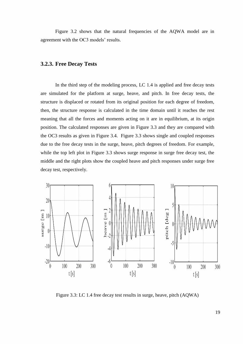
3.2.3. Free Decay Tests
In the third step of the modeling process, LC 1.4 is applied and free decay tests
are simulated for the platform at surge, heave, and pitch. In free decay tests, the
structure is displaced or rotated from its original position for each degree of freedom,
then, the structure response is calculated in the time domain until it reaches the rest
meaning that all the forces and moments acting on it are in equilibrium, at its origin
position. The calculated responses are given in Figure 3.3 and they are compared with
the OC3 results as given in Figure 3.4. Figure 3.3 shows single and coupled responses
due to the free decay tests in the surge, heave, pitch degrees of freedom. For example,
while the top left plot in Figure 3.3 shows surge response in surge free decay test, the
middle and the right plots show the coupled heave and pitch responses under surge free
decay test, respectively.
Figure 3.3: LC 1.4 free decay test results in surge, heave, pitch (AQWA)

20
Figure 3.4: LC 1.4 free decay test results in the surge, heave, pitch (OC3)
(source: Jonkman and Musial 2010)
Figure 3.4 shows that the calculated response results of the current model fit the
results of other participant’s free decay tests.
3.2.4. Hydrodynamic Response with Regular Waves
The next step of the modeling is the investigation of the time-domain response
of the spar-type FOWT model under the regular wave load case, LC 4.1. The wave
height, H, is 6m, and the wave period, T, is 10 sec. in the regular wave case applied in
OC3. The wave incident angle is zero degrees showing the positive x-direction. Under
that load case, the surge, heave, and pitch degrees of freedom are taken into
consideration in the analysis since they are the only ones excited under zero degrees
wave incidence. The dynamic behavior of the structure is investigated under LC 4.1,
time histories of the surge and heave displacements, pitch rotation, and seaward cable

21
tension are simulated and compared with OC3 results.AQWA model time responses are
given in Figure 3.5, and OC3 results are given in Figure 3.6 for comparison.
Figure 3.5: LC 4.1 time-domain response analysis results for AQWA model
Figure 3.6:: LC 4.1 time-domain response analysis results for OC3 participants
(source: Jonkman and Musial 2010)

22
Figure 3.5 indicates that the surge, heave, pitch responses are in agreement with
OC3 results in Figure 3.6 as well as fairlead tension responses. HAWC2 model’s
discrepancy in the surge is attributed to an error in the output parameter as mentioned in
Jonkman and Musial (2010).
3.2.5. Hydrodynamic Response with Irregular Waves
The frequency-domain response of the structure is investigated in the last step of the
numerical modeling. Irregular wave parameters are given as input to AQWA.
According to LC 4.2, the significant wave height is 𝐻𝑠 = 6 𝑚, the peak period is, 𝑇𝑝 =
10 𝑠, and the irregular wave series are generated using the JONSWAP spectrum. The
wave incident angle is zero degrees showing the positive x-direction, The wave load
under zero degree incidence excites the model in the surge, pitch, heave degrees of
freedom, and tension forces occur on mooring lines, same as LC 4.1. Platform responses
in the relevant DOFs are shown as using energy spectra in the frequency domain. The
results for the AQWA model are given in Figure 3.7 and the results of OC3 participants
are given in Figure 3.8, on a logarithmic scale.
Figure 3.7: LC 4.2 frequency domain response analysis results for AQWA model
23
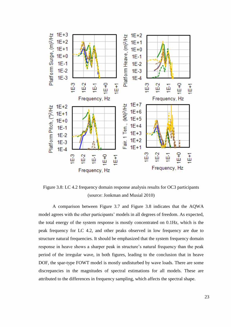
Figure 3.8: LC 4.2 frequency domain response analysis results for OC3 participants
(source: Jonkman and Musial 2010)
A comparison between Figure 3.7 and Figure 3.8 indicates that the AQWA
model agrees with the other participants’ models in all degrees of freedom. As expected,
the total energy of the system response is mostly concentrated on 0.1Hz, which is the
peak frequency for LC 4.2, and other peaks observed in low frequency are due to
structure natural frequencies. It should be emphasized that the system frequency domain
response in heave shows a sharper peak in structure’s natural frequency than the peak
period of the irregular wave, in both figures, leading to the conclusion that in heave
DOF, the spar-type FOWT model is mostly undisturbed by wave loads. There are some
discrepancies in the magnitudes of spectral estimations for all models. These are
attributed to the differences in frequency sampling, which affects the spectral shape.

24
CHAPTER 4
4. WAVE GENERATION AND ANALYSIS IN THE
LABORATORY
4.1. Wave Environment
To conduct physical model experiments, waves should be generated and
analyzed in the laboratory. This study is intended to stimulate, generate and analyze
different wave conditions in a laboratory environment. To that end, datasets consisting
of regular or irregular wave time series are used. Moreover, the frequency spectrum is
used to describe irregular waves in the frequency domain.
4.1.1. Regular Waves
Adhering to the linearized Airy wave theory, regular waves are described as the
most basic form of a monochromatic wave (a wave with one distinct frequency and
wave height). Under the simplifying assumptions that the fluid is irrotational, inviscid,
and incompressible, surface profile solution is derived from the Laplace equation for an
ideal fluid:
𝜂 = 𝑎 ∙ cos (𝑘𝑥 − 𝜔𝑡 + 𝜖) (4.1)
and;
𝑘 =
2𝜋
𝐿; 𝜔 =
2𝜋
𝑇
(4.2)
where 𝜂 denotes water surface profile, 𝑎 is the wave amplitude and is the half of
the wave height, 𝐿 is the wavelength, 𝑇 is the wave period, 𝑘 is the wavenumber, 𝜔 is
the wave angular frequency, 𝑡 is the time, 𝑥 is the cartesian coordinate in the horizontal
axis, and 𝜖 is the phase of the wave. An example of the water surface profile is given in
Figure 4.1.

25
Figure 4.1: Regular wave
The dispersion relation is given as:
𝜔2 = 𝑔𝑘𝑡𝑎𝑛ℎ(𝑘ℎ) (4.3)
where 𝑔 represents the gravitational acceleration
A definitive assumption of the Airy wave theory is that wave height is smaller
when compared to the water depth and wavelength. Those assumptions linearize the
boundary conditions as well as neglecting the higher-order terms, making the solution
correct to the first order.
Regular waves are, of course, not encountered in nature. However, their simplicity
provides good initial approximations in laboratory experiments as well as numerical
studies. Also, regular waves are important when irregular waves are being investigated
as they are considered the components of irregular wave series.

26
4.1.2. Irregular Waves
In laboratory conditions, regular waves can be generated relatively easily.
Although being useful in preliminary tests, those waves won’t be representative of any
real-world simulations. To get a closer approximation to the waves that are observable
in nature, irregular waves must be generated.
Irregular waves are often described as the superposition of an infinite number of
regular (monochromatic) waves. When the surface profile of a random sea is plotted in
the time domain, the resulting form may seem random, however, the same time series
can also be investigated in the frequency domain using a Fourier Transform (FT)
scheme, which will yield the accumulated wave energies under discrete frequencies,
also known as “the spectrum”. Over time, numerous spectra are modeled, using the
gathered ocean data. An overview of wave spectra is given in the literature review (
Chapter 2). Hasselmann (1973) realized fetch limited waves shows characteristically
sharper peaks than fully developed PM spectrum, and introduced a “peak enhancement
factor” in the definition of the spectrum to better capture this phenomenon. The general
expression of wave spectra, given in terms of wave height and period by Goda (1988),
is used in this study, which can be used to generate different types of the spectrum such
as JONSWAP or Pierson-Moskowitz by changing the input parameters:
𝑆(𝑓) = β𝐻𝑠
2𝑇𝑝1−𝑚𝑓−𝑚 exp [−
𝑚
𝑛(𝑇𝑝𝑓)
−n] 𝛾
exp[−(𝑇𝑝𝑓−1)
2
2𝜎2 ]
(4.4)
and;
β ≅
0.0624 (1.094 − 0.01915 ln 𝛾)
0.230 + 0.0336 𝛾 − 0.185(1.9 + 𝛾)−1 (4.5)
𝛾 = 1~7, 𝜎 ≅ {
0.07: 𝑓 ≤ 𝑓𝑝,
0.09: 𝑓 > 𝑓𝑝. (4.6)
where, 𝐻𝑠 denotes significant wave height which corresponds to the mean value of 1/3th
of all individual wave heights in the zero-up crossing method, 𝑇𝑝 is the peak period in
the wave spectrum, 𝛾 is the aforementioned peak enhancement factor which can be
ranged between 1 to 7 with a typically used mean value of 3.3, 𝑓 denotes the discrete

27
frequencies in the spectrum, and 𝑓𝑝 is spectral peak frequency which is the
multiplicative reciprocal of 𝑇𝑝. When 𝑚 and 𝑛 are equal to 5 and 4, respectively, and 𝛾
is equal to 1.0, Eq. 4.4 gives the the definition of PM spectrum. The comparison of PM
and JONSWAP spectra with 𝛾 =3.3 is given in Figure 4.2.
Figure 4.2: A comparison of PM and JONSWAP spectrum with the same wave
parameters (Hs=1.5m, Ts=7.6s)
4.2. Analysis Procedures of Wave Datasets
Being able to process the wave data is important to understand the properties of
the wave train, and it is also a critical step in the synthesis of random waves. Several
methods will be described here used in the analysis of time series of random waves
which are either generated theoretically or measured during the tests of laboratory
experiments. The procedures to obtain the frequency spectrum from time-domain data
and to derive irregular wave properties from created spectra are explained. Being able to
process the data in time and frequency domains opens up the possibility to obtain
28
entirely random wave time series with desired wave characteristics. These procedures
also enable the user to make proper validations between theoretical results and
experimental ones.
4.2.1. Frequency Domain Analysis
The most basic form of a sine wave, also known as a regular wave, can be
described with a trigonometric function consisting of wave amplitude and wave period.
However, that function is never going to properly define realistic wave profiles.
Fortunately, irregular waves as seen in nature can be idealized as the superposition of an
infinite number of regular waves, which brings the possibility to decompose the
irregular wave series to its regular wave components. An irregular wave consisting of
an infinite regular wave series with many frequencies, amplitudes, and phases can be
mathematically described as a time-dependent function:
𝑥(𝑡) = ∑ 𝑎𝑛cos (𝜔𝑛𝑡 − 𝜖𝑛)
∞
𝑛=0
(4.7)
where 𝑎𝑛 denotes wave amplitude, 𝜔𝑛 angular wave frequency, and 𝜖𝑛 the phase
of each wave in the time domain.
Using the Eulerian identity:
𝑒𝑖𝜃 = 𝑐𝑜𝑠𝜃 + 𝑖𝑠𝑖𝑛𝜃 (4.8)
Fourier transform in the complex form can be defined:
𝑋(𝜔) = 𝐴(𝜔) − 𝑖𝐵(𝜔) (4.9)
and,
𝐴(𝜔) =
1
2𝜋∫ 𝑥(𝑡)𝑐𝑜𝑠𝜔𝑡𝑑𝑡
∞
−∞
𝐵(𝜔) =1
2𝜋∫ 𝑥(𝑡)𝑠𝑖𝑛𝜔𝑡𝑑𝑡
∞
−∞
(4.10)
where 𝐴(𝜔) and 𝐵(𝜔) here are two continuous components of the Fourier transform.
Substituting Eq. (4.10) into Eq. (4.9) and using the Eulerian identity in Eq. (4.8) yields:

29
𝑋(𝜔) =
1
2𝜋∫ 𝑥(𝑡)(𝑐𝑜𝑠𝜔𝑡 − 𝑖𝑠𝑖𝑛𝜔𝑡)𝑑𝑡
∞
−∞
=1
2𝜋∫ 𝑥(𝑡)𝑒−𝑖𝜔𝑡𝑑𝑡
∞
−∞
(4.11)
Eq. (4.11) is the complex representation of the Fourier transform and can be used
effectively to describe the time-domain function in the frequency domain. Fourier
transforms can also be used to convert functions in the frequency domain to time
domain representations using the form termed as ‘inverse Fourier transform’. Inverse
Fourier transform is described in the complex form as:
𝑥(𝑡) = ∫ 𝑋(𝜔)𝑒𝑖𝜔𝑡𝑑𝜔
∞
−∞
(4.12)
Using Fourier transform in a procedure known as ‘Fast Fourier Transform’
‘FFT’ allows the user to calculate the discrete Fourier transform of a periodic process
with 𝑁 discrete data points, resulting spectral coefficients are in the complex form of:
𝑋𝑛 = 𝑎 − 𝑖𝑏 ; 𝑛 = 0,1, … , (𝑁 − 1) (4.13)
At the discrete frequency points in which 𝑎 and 𝑏 are the Fourier components and the
magnitude of the spectral amplitudes can be calculated as:
𝑆𝑛 = 𝑋𝑛 ∙ 𝑋𝑛∗ ; 𝑛 = 0,1, … , (𝑁 − 1) (4.14)
where 𝑋𝑛∗ is the complex conjugate of the spectral coefficients, and 𝑆𝑛 is the spectral
amplitude, also known as ‘magnitude’, at 𝑛’th discrete frequency. Frequency sampling
in an FFT scheme is directly dependent on the time step of the discrete-time series:
𝑓𝑛 = 𝑛 ∙ 𝑑𝑓 𝑑𝑓 = 1/𝑁∆𝑡
; 𝑛 = 0,1, … , (𝑁 − 1) (4.15)
where ∆𝑡 denotes the time step, 𝑑𝑓 is the sampling frequency, and 𝑓𝑛 the discrete
frequency at the 𝑛’th point in the series. The frequency spectrum is created when the
resulting spectral amplitudes are plotted against the discrete frequencies. Since the area
under the energy spectrum represents the total wave energy, when the energy spectrum
is plotted for wave measurement taken at discrete time steps, the resulting plot will give
ideas about the frequencies where the wave energies are the most dominant. If FFT is
applied and the spectrum is plotted for a regular wave, the spectrum will show one peak
as there is just one wave frequency and all wave energy is concentrated there, but for an
irregular wave train, the frequency spectrum will show the distribution of different
energy levels on different discrete frequencies. Time series and frequency spectrum

30
examples of a bichromatic wave (two regular waves with different frequencies) and an
irregular wave are given in Figure 4.3
Figure 4.3: Time series (left) and spectra (right) of a bichromatic wave (up) and an
irregular wave (down)
Many programming languages offer built-in methods for FFT calculations.
Details of the FFT technique can be found in Newland (2012).
4.2.2. Spectral moments

31
It is also possible to extract the wave characteristics from the spectral description
of the sea waves. Representative wave heights and periods can be derived from the
wave energy spectrum. The concept of spectral moments is used to that end, and its
definition for the 𝑛th moment of the spectrum is given as (Mackay 2012):
𝑚𝑛 = ∫ 𝑓𝑛𝑆(𝑓)𝑑𝑓
∞
0
(4.16)
here, 𝑚𝑛 describes the 𝑛th moment of the spectrum, 𝑓 is frequency and 𝑆(𝑓) is
the value of the energy spectrum function at the frequency, 𝑓.
It is mentioned earlier that the area under the energy spectrum represents the total
wave energy. The area under the spectrum function can be found by integrating it over
the frequency range. In other words, total wave energy should correspond to 𝑚0, the
zeroth moment of the spectrum. A practical approach to calculate the area is using the
so-called “trapezoid rule”. It is a simple and efficient procedure and many programming
languages offer libraries with built-in functions that include this procedure.
Other relationships between spectral moments and wave parameters are given as:
𝐻𝑚0 ≈ 4.004√𝑚0 (4.17)
�̅� = √𝑚0
𝑚2 (4.18)
𝑇𝑝 =
1
𝑓𝑝 (4.19)
the frequency corresponding to the peak point of the spectrum function is termed peak
frequency, 𝑓𝑝 and reciprocal of 𝑓𝑝 yield the peak period, 𝑇𝑝.
4.2.3. Time Domain Analysis
For the time domain analysis, the zero-up crossing method is widely used to
determine the individual waves in irregular wave time series. Initially, the mean water
level is determined by averaging the whole water surface profile and defined as the zero
lines or still water level. Then, starting from the beginning of the wave record, points
are searched where the surface profile crosses the zero line upward. The surface profile

32
between two consecutive zero-up crossing points is taken as one individual wave. The
difference between the maximum and the minimum of water surface elevation in each
wave is noted as the individual wave height. The duration between the starting and
ending points of each wave is noted as the corresponding individual wave period. Using
zero-up crossing methods all of the individual wave heights and their corresponding
wave periods are calculated.
After the determination of the individual waves, some characteristic waves should
be defined for an irregular wave environment. To determine the characteristic waves of
the time series, individual waves calculated by the zero-up crossing method are sorted
in descending order according to the wave heights. While the wave height of the highest
wave in the wave record is denoted 𝐻𝑚𝑎𝑥 , the period corresponding to 𝐻𝑚𝑎𝑥 is named
𝑇𝑚𝑎𝑥. Mean wave heights and periods are calculated using all waves in the wave record,
and they are denoted �̅� and �̅�, respectively. The highest one-third wave (33%), also
known as the significant wave is defined as the mean values of wave heights and
periods of the highest one-third of the individual waves in the wave record. They are
denoted as 𝐻1/3 and 𝑇1/3 or 𝐻𝑠 and 𝑇𝑠, respectively. Significant wave heights and
periods are important because they are the most frequently used characteristic waves in
the various coastal engineering activities like the stability of the rubble mound. In this
study, the zero-up crossing method is used in the validation process of the synthesis of
random waves and the calculation of measured wave properties of the waves generated
in the laboratory experiments.
4.3. Preparation of the Wave Generator Signal
In this study, the deterministic spectral amplitude method is used in the random
generation of irregular wave time series. In this section, the “Deterministic spectral
amplitude method (DSA)” is explained and an example is provided as well as the
validation used in the process. Next, the wavemaker theory is given and solutions are
provided to the first and second-order for regular and irregular waves. A flow chart
describing the steps in the generation of waves for the laboratory experiments is
provided in Figure 4.4.

33
Figure 4.4: Flow chart describing the steps involving wave generation
4.3.1. Synthesis of the Irregular Wave Series
To synthesize irregular waves, the Deterministic Spectral Amplitude (DSA)
method (Tuah and Hudspeth,1982) is used in this study. This method allows the
synthesis of irregular wave time series that have the spectral properties of a targeted
spectrum. The premise of the adopted wave synthesis scheme is that as the frequency

34
spectrum can be obtained from wave time series using FFT, inversely, time series can
be generated from any given spectra. Moreover, time-domain representations of any
wave consist of two elements; amplitude and phase, and yet, due to the nature of Fourier
transformation, phase knowledge of the series is lost after the application of FFT.
Therefore, to synthesize a new wave time series, the DSA model proposes to use
randomly generated phases to be included in the inverse Fast Fourier Transform (iFFT).
This method effectively makes it possible to generate an infinite number of irregular
wave series that all adhere to the targeted spectral form. In the application of the method
the followed steps are explained below;
1 – Using significant wave height, and peak spectral frequency as inputs, a target
spectrum is formed using Eq. (4.4)
2 – With a random number generator, a phase sequence of zero mean and unit
variance is generated in the range between 0 to 2π
3 – Fourier coefficients are calculated using the relation given below:
𝐴𝑛 = 𝑁 (𝑆(𝑓𝑛)𝑑𝑓
2)
0.5
𝑒𝑖𝜃𝑛 𝑛 = 1,2, … , 𝑁 (4.20)
where 𝑁 is the total number of discrete data points, 𝑆(𝑓𝑛)is the wave spectral
density at 𝑛th frequency, 𝑑𝑓 is the frequency sampling rate, 𝜃𝑛 is the 𝑛th phase in the
randomly generated phase sequence, and 𝐴𝑛 denotes the Fourier coefficients.
4 – Fourier coefficients sequence are extended by mirroring 𝐴𝑛 series with the
complex conjugate of 𝐴𝑛
5 – Inverse FFT (iFFT) is applied to the Fourier coefficients, which, in the end,
generates 2𝑁 number of discrete water surface profile values from 𝑁 number of discrete
wave energy spectrum.
The method is reported to produce realistic water surface profiles for large N
Wang and Crouch (1993). Also, to increase efficiency in the FFT scheme, the value of
𝑁 is always chosen as 2𝑚.
After synthesizing the random wave series, a two-step validation process is
applied by a computer program written in house. First, the wave energy spectrum is re-
derived from the synthesized random irregular wave. The re-derived wave spectrum is

35
compared to the target spectrum. Second, the zero-up crossing is applied to the random
wave time series to calculate the characteristic wave height and periods. The same wave
properties are also calculated from the spectral moments of the obtained wave energy
spectrum, and those are compared to the zero-up crossing results. It is known that the
wave height calculated using Eq.(4.17) from the spectrum (𝐻𝑚0) should be close to
significant wave height, Hs calculated from the time series by the zero-up crossing
method. Furthermore, the relation between the peak period (𝑇𝑝) and the siginificant
wave period (𝑇𝑠) defined by Mitsuyasu (1970) is checked using the formula given
below:
𝑇𝑝 = 1.05𝑇𝑠 (4.21)
If the comparisons in both steps agree with each other, then it can be concluded
that the spectrum function is applied correctly in the program and the generated random
irregular wave exhibits the targeted wave characteristics.
An example of irregular wave generation is provided with parameters 𝑇𝑝 = 1.5𝑠,
𝐻𝑠 = 0.25𝑚. The frequency spectrum type is JONSWAP with 𝛾 = 3.3 . The total
number of discrete data points is chosen as, 𝑁 = 8192, and the time step is ∆𝑡 = 0.01𝑠.
The time series for the water surface profile is given in Figure 4.5.
Figure 4.5: Randomly generated irregular wave series

36
To validate the wave generation scheme, the theoretical target spectrum is compared to
the spectrum derived from the irregular wave time series given in Figure 4.6.
Figure 4.6: Comparison of the theoretical spectrum obtained by Eq.(4.4)(left), and the
one obtained from the synthesized irregular waves (right)
As can be seen in Figure 4.6, the spectrum obtained from the synthesized time
series and the theoretical spectrum are the same. This verifies that the DSA method is
applied correctly in this study. Table 4.1 provides the comparison of the wave properties
from both spectral moments and zero-up crossing of the random wave time series.
Ratios of the differences between 𝐻𝑠 and 𝑇𝑚𝑒𝑎𝑛 values are checked and found to be
within acceptable parameters that are rough ~5% and ~7% (Goda, 1979; 2000).
Table 4.1: Validation of the wave generation scheme with spectral and statistical
parameters
Parameters Values Derived From Spectral
Moments
Statistical Values From Zero-
up Crossing
𝐻𝑠 0.20 m 0.195 m
𝑇𝑠 1.90 s 1.88 s
𝑇𝑚𝑒𝑎𝑛 1.55 s 1.54 s

37
4.3.2. Wave Board Displacement Functions by Wavemaker Theory
The foundation of the theory of wavemakers was led by Havelock (1929),
considering the waves as the vertical oscillations of the water surface forced by a planar
or cylindrical solid body. The theory was later extended by Biesel (1951), which
provided solutions to different types of wave generators such as piston or flap type.
Then, the theory has been improved extensively for both regular (Fontanet 1961) and
irregular waves (Sand and Mansard, 1986; Schäffer, 1996). A sketch for the generalized
wave generator in a two-dimensional wave flume is given in Figure 4.7.
Figure 4.7: A 2-D sketch of the generalized wave generator system
(source: Schäffer 1996)
Wave generators may force the water waves with translational or rotational
motion, or a combination of the two. Assumptions are made that the fluid is
incompressible, inviscid, and irrotational, surface tension is neglected, the bed of the
flume is horizontal, flat, and impermeable. Also, the condition at the wave board is that
the velocity gradient normal to the surface of the wave board is equal to the velocity of
the fluid in the same direction. Laplace equation in two dimensions is used in a
Cartesian coordinate system and is assumed to describe the motion of the fluid in the

38
wave flume. Following boundary conditions and boundary value problems are given
below, adhering to the notation used by Barthel et al. (1983) and (Schäffer 1996):
Let 𝜙 = 𝜙(𝑥, 𝑧, 𝑡) define the velocity potential and 𝑢 = 𝜙𝑥, 𝑣 = 𝜙𝑧
Laplace equation:
∆𝜙 = 0 𝑒𝑣𝑒𝑟𝑦𝑤ℎ𝑒𝑟𝑒 (4.22)
Dynamic free surface condition:
𝜙𝑡 +
1
2(𝜙𝑥
2 + 𝜙𝑧2) + 𝑔𝜂 = 0
𝑓𝑜𝑟 𝑧 = 𝜂 (4.23)
Kinematic free surface condition:
𝜂𝑡 + 𝜙𝑥𝜂𝑥 − 𝜙𝑧 = 0 𝑓𝑜𝑟 𝑧 = 𝜂 (4.24)
Impermeable bottom condition:
𝜙𝑧 = 0 𝑓𝑜𝑟 𝑧 = −ℎ (4.25)
Wave board condition:
𝜙𝑥 = (1 +𝑧
ℎ + 𝑙) 𝑋𝑜𝑡
𝑓𝑜𝑟 𝑥 = 𝑋(𝑧, 𝑡) (4.26)
where 𝜂 = 𝜂(𝑥, 𝑡) is the water surface elevation, 𝑔, ℎ, 𝑎𝑛𝑑 𝑡 are the gravitational
acceleration, water depth, and time, respectively. h, l, and z are shown in Figure 4.7.
The wave board position is given as:
𝑋(𝑧, 𝑡) = 𝑓(𝑧) 𝑋0(𝑡) (4.27)
where 𝑓(𝑧) is a function that describes the type of wavemaker:
𝑓(𝑧) = {
1 +𝑧
ℎ + 𝑙 𝑓𝑜𝑟 − (ℎ − 𝑑) ≤ 𝑧 ≤ 0
0 𝑓𝑜𝑟 − ℎ ≤ 𝑧 < −(ℎ − 𝑑) (4.28)
where 𝑧 = −(ℎ + 𝑙) is used to describe the center of rotation and 𝑑 ≥ 0 is the elevation
of the hinge over the bottom. For a piston-type wavemaker, the center of rotation has
the limit 𝑙 → ∞ and 𝑑 = 0, making the second case in (4.28) inapplicable.
The solution scheme for this problem requires the Taylor series expansion to be applied
to the Eqs. (4.23) - (4.26), which will yield boundary conditions at 𝑥 = 0 and 𝑧 = 0.
Next, using the perturbation theory, the terms 𝜙, 𝜂, and 𝑋0 are rewritten as perturbation
series:

39
𝜙 = 𝜖𝜙(1) + 𝜖2𝜙(2) (4.29)
𝜂 = 𝜖𝜂(1) + 𝜖2𝜂(2) (4.30)
𝑋0 = 𝜖𝑋0(1) + 𝜖2𝑋0
(2) (4.31)
where 𝜖 is the small ordering parameter that is proportional to wave steepness (Flick
and Guza 1980). The solution procedure yields the resulting boundary value problems:
𝜙𝑡𝑡 + 𝑔𝜙𝑧 = 𝑅 𝑓𝑜𝑟 𝑧 = 0 (4.32)
𝜙𝑥 = 𝑄 𝑓𝑜𝑟 𝑥 = 0 (4.33)
𝜂 =1
𝑔(𝜙𝑡 + 𝑃) 𝑓𝑜𝑟 𝑧 = 0 (4.34)
𝜙𝑧 = 0 𝑓𝑜𝑟 𝑧 = −ℎ (4.35)
for the first-order problem 𝑅, 𝑄 and 𝑃 becomes for (𝜙, 𝜂) = (𝜙(1), 𝜂(1)):
𝑅(1) = 0 (4.36)
𝑄(1) = 𝑓(𝑧)𝑋0𝑡(1)
(4.37)
𝑃(1) = 0 (4.38)
and for the second-order problem 𝑅, 𝑄 and 𝑃 becomes for (𝜙, 𝜂) = (𝜙(2), 𝜂(2)):
𝑅(2) = − {(𝜙𝑥(1)2
+ 𝜙𝑧(1)2
)𝑡
+ 𝜂(1) (𝜙𝑡𝑡(1)
+ 𝑔𝜙𝑧(1)
)𝑧} (4.39)
𝑄(2) = −𝑋0
(1){𝑓(𝑧)𝜙𝑥𝑥
(1)−
1
ℎ + 𝑙𝜙𝑧
(1)} + 𝑓(𝑧)𝑋0𝑡
(2) (4.40)
𝑃(2) =
1
2(𝜙𝑥
(1)2
+ 𝜙𝑧(1)2
) + 𝜂(1)𝜙𝑧𝑡(1)
(4.41)
4.3.2.1. Spurious Harmonic Waves
Before proceeding to the solution of the wavemaker problem, it is worth
mentioning the spurious harmonic waves. In the solution of the wavemaker problem to
the second-order, due to the linearity of the boundary value problems Barthel et al.
(1983) rewrote 𝜙(2) as the superposition of three components:
𝜙(2) = 𝜙(21) + 𝜙(22) + 𝜙(23) (4.42)
where the 𝜙(21) gives the second-order bound long waves and the solution of it
describes the progressive waves. Boundary conditions that 𝜙(22) have to satisfy contain

40
terms that correspond to spurious waves which should not be on a natural wave train.
One term that occurs due to the local disturbances is termed as “local disturbance
waves”, another free long wave that arose due to the wave board leaving its mean
position is termed “displacement wave”, and the third free wave which is generated due
to the negative component of the progressive wave which represents the orbital velocity
reflecting off the wave board surface is termed the “parasitic long wave”. Therefore, to
eliminate those spurious long waves 𝜙(23) must have the condition:
𝜙(22) + 𝜙(23) = 0 (4.43)
in other words, to eliminate the spurious-free waves, the second-order wavemaker
solution must determine 𝑋0(2)
(𝑡) so that 𝜂0(23)
should satisfy:
𝜂0(22)
+ 𝜂0(23)
= 0 (4.44)
In that pattern, the boundary value problems in Eq. (4.39)-(4.41) become:
for (𝜙, 𝜂) = (𝜙(21), 𝜂(21) ):
𝑅(21) = − {(𝜙𝑥
(1)2+ 𝜙𝑧
(1)2)
𝑡+ 𝜂(1) (𝜙𝑡𝑡
(1)+ 𝑔𝜙𝑧
(1))
𝑧} (4.45)
𝑄(21) = 𝑎𝑟𝑏𝑖𝑡𝑟𝑎𝑟𝑦 (4.46)
𝑃(21) =
1
2(𝜙𝑥
(1)2+ 𝜙𝑧
(1)2) + 𝜂(1)𝜙𝑧𝑡
(1) (4.47)
for (𝜙, 𝜂) = (𝜙(22), 𝜂(22) ):
𝑅(22) = 0 (4.48)
𝑄(22) = {−𝑋0
(1){𝑓(𝑧)𝜙𝑥𝑥
(1)−
1
ℎ + 𝑙𝜙𝑧
(1) } − 𝜙𝑥
(21), 𝑓𝑜𝑟 − (ℎ − 𝑑) ≤ 𝑧 ≤ 0
𝜙𝑥(21)
, 𝑓𝑜𝑟 − ℎ ≤ 𝑧 < −(ℎ − 𝑑)
(4.49)
𝑃(22) = 0 (4.50)
and for (𝜙, 𝜂) = (𝜙(23), 𝜂(23) ):
𝑅(23) = 0 (4.51)
𝑄(23) = 𝑓(𝑧)𝑋0𝑡(2)
(4.52)
𝑃(23) = 0 (4.53)
In the solution provided by Barthel et al. (1983) only the difference frequencies
are deemed of interest because they produce long wave terms. However, a later study by
Sand and Mansard (1986) showed that summation frequencies also have free harmonic

41
contributions that must be dealt with, and also, a wavemaker theory that includes
summation frequencies produces more realistic waves with sharper crests and flatter
throughs. Sand and Mansard (1986) also generalized the terms given by Barthel et al.
(1983) to “subharmonics” for difference frequency terms and “superharmonics” for
summation frequency terms.
4.3.2.2. Generation of Regular Waves
Due to the simpler theoretical nature of regular waves, wave board solution in the
wavemaker theory was established firstly. The solution was provided by considering the
boundary value problems in Eq. (4.32) to Eq.(4.35), then applying the separation of
variables technique to separate the Laplace equation into ordinary differential equations
with known solutions. Summation of the solutions where the separation constant is real
𝑘12 > 0, 𝑘2 = 0, and imaginary 𝑘3
2 < 0, gives the solution to the general velocity
potential function (Flick and Guza 1980):
𝜙(1)(𝑥, 𝑧, 𝑡) = 𝐴 cosh[𝑘1(ℎ + 𝑧)] sin(𝑘1𝑥 − 𝜔𝑡)
+ cos 𝜔𝑡 ∑ 𝐶𝑛𝑒−𝑘3𝑛𝑥cos [𝑘3𝑛(𝑧 + ℎ)]
∞
𝑛=1
(4.54)
and,
𝐴 =𝜔𝑆0 ∫ 𝑓(𝑧) cosh[𝑘1(ℎ + 𝑧)]𝑑𝑧
0
−ℎ
2𝑘1 ∫ cosh2[𝑘1(ℎ + 𝑧)]𝑑𝑧0
−ℎ
(4.55)
𝐶𝑛 =𝜔𝑆0 ∫ 𝑓(𝑧) cos[𝑘3𝑛
(ℎ + 𝑧)]𝑑𝑧0
−ℎ
2𝑘3𝑛∫ cos2[𝑘3𝑛
(ℎ + 𝑧)]𝑑𝑧0
−ℎ
(4.56)
where 𝑆0 denotes the wave board stroke at 𝑧 = 0 and:
𝑋0
(1)=
𝑆0
2sin 𝜔𝑡 (4.57)
water surface elevation in the wave flume is found as:
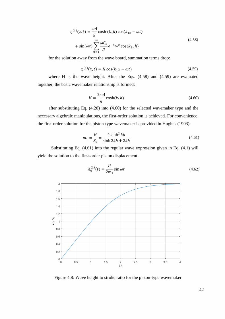
42
𝜂(1)(𝑥, 𝑡) =
𝜔𝐴
𝑔cosh (k1ℎ) cos(𝑘1𝑥 − 𝜔𝑡)
+ sin(𝜔𝑡) ∑𝜔𝐶𝑛
𝑔𝑒−𝑘3𝑛𝑥 cos(𝑘3𝑛
ℎ)
∞
𝑛=1
(4.58)
for the solution away from the wave board, summation terms drop:
𝜂(1)(𝑥, 𝑡) = 𝐻 cos(𝑘1𝑥 − 𝜔𝑡) (4.59)
where H is the wave height. After the Eqs. (4.58) and (4.59) are evaluated
together, the basic wavemaker relationship is formed:
𝐻 =
2𝜔𝐴
𝑔cosh(𝑘1ℎ) (4.60)
after substituting Eq. (4.28) into (4.60) for the selected wavemaker type and the
necessary algebraic manipulations, the first-order solution is achieved. For convenience,
the first-order solution for the piston-type wavemaker is provided in Hughes (1993):
𝑚1 =
𝐻
𝑆0=
4 sinh2 𝑘ℎ
sinh 2𝑘ℎ + 2𝑘ℎ (4.61)
Substituting Eq. (4.61) into the regular wave expression given in Eq. (4.1) will
yield the solution to the first-order piston displacement:
𝑋0
(1)(𝑡) =
𝐻
2𝑚1sin 𝜔𝑡 (4.62)
Figure 4.8: Wave height to stroke ratio for the piston-type wavemaker

43
The phase terms from Eq. (4.1) are not shown for the sake of simplicity. Figure
4.8 shows the wave height to stroke ratio with relative depth for the piston-type
wavemaker. It can be seen that the piston-type wave generator’s efficiency reaches its
maximum at deepwater conditions.
Second-order derivations to the wavemaker problem suggest that the attempts to
generate waves in laboratory conditions using the first-order solution will produce
unwanted harmonics in the wave flume. It can be seen by observations from Goda
(1967) that those spurious-free waves distort the wave record and this effect becomes
more dominant as the steepness of the waves 𝐻/𝐿 increases or the relative depth ℎ/𝐿
decreases (Hughes 1993). An approximate second-order wavemaker theory for regular
waves developed by Madsen (1970) and Madsen (1971) requiring:
𝜙(2) = 𝜙(21) + 𝜙(22) (4.63)
It is worth to reaccent that in this notation 𝜙(21) describes the second-order bound
waves naturally occurring with the wave groups, traveling with the group velocity and
𝜙(22) describes the spurious effects. The objective of the solution to the velocity
potential, 𝜙(2) is to obtain 𝜙(23) which gives the relationship in Eq.(4.43). Solving
𝜙(23) for 𝑋0 will give the wave generator signal required to compensate for the spurious
harmonic waves in the generated wave series. Substituting 𝜙(21) in Eq. (4.63) into the
second-order boundary value problems in Eq.(4.45) - (4.47) and substituting 𝜙(22) in
Eq. (4.63) into the second-order boundary value problems in Eq.(4.48) - (4.50) yields
two important terms:
𝜙(21)(𝑥, 𝑧, 𝑡) =
3𝜔𝐻2
32
cosh 2𝑘(ℎ + 𝑧)
sin4 𝑘ℎsin 2(𝑘𝑥 − 𝜔𝑡) (4.64)
and,
𝜙𝑥
(22)= (1 −
ℎ
2(ℎ + 𝑙)) 𝑋0𝑡
(2)+
𝜔𝐻2
16ℎ(
2
𝑚1−
3 cosh 𝑘ℎ
sinh3 𝑘ℎ) cos 2𝜔𝑡 (4.65)
After solving the boundary value problems for 𝜙(21) and 𝜙(22) Madsen (1971)
described the second-order wave in terms of the first-order wave, second-order bound
wave, and the second-order spurious-free wave. Thus the combined wave board solution
becomes:

44
𝑋0(𝑡) = 𝑋0(1)
+ 𝑋0(2)
(4.66)
where 𝑋0(1)
is the first-order wavemaker solution given in Eq. (4.62), 𝑋0(2)
is the
second-order wavemaker solution to compensate for the spurious-free wave, and 𝑋0(𝑡)
is the combined second-order wavemaker solution for regular waves. Solution to
𝑋0(2)
and 𝑋0(𝑡) are given as:
𝑋0
(2)(𝑡) =𝐻2
32ℎ (1 −ℎ
2(ℎ + 𝑙))
(3 cosh 𝑘ℎ
sinh3 𝑘ℎ−
2
𝑚1) 𝑠𝑖𝑛2𝜔𝑡
(4.67)
𝑋0(𝑡) =
𝐻
2𝑚1sin 𝜔𝑡 +
𝐻2
32ℎ (1 −ℎ
2(ℎ + 𝑙))
(3 cosh 𝑘ℎ
sinh3 𝑘ℎ−
2
𝑚1) 𝑠𝑖𝑛2𝜔𝑡 (4.68)
As an example, a piston displacement solution is provided for the second-order regular
wave. Parameters are set as; wave height, 𝐻 = 0.2𝑚, wave period, 𝑇 = 5𝑠, depth, ℎ =
1𝑚, solving Eq. (4.3) for the wavenumber, and yields 𝑘 = 0.412. using Eq. (4.2),
remaining parameters, angular frequency, and wavelength are obtained as, 𝜔 = 1.26 ,
and 𝐿 = 15.24𝑚 . Using Eq. (4.52) 𝑚1 = 0.412. This is consistent with Figure 4.8, as
for very shallow water conditions the relationship is similar to 𝑚1 ≈ 𝑘ℎ. After that, Eq.
(4.68) is applied to obtain the necessary wave board motion required to generate the
targeted regular wave. The first-order and second-order contributions to the combined
wave board motion are also obtained from Eq. (4.62) and (4.67) for demonstration
purposes, and they are shown in Figure 4.9.
Figure 4.9: Second-order wave board displacement for a regular wave

45
4.3.2.3. Generation of Irregular Waves
It has been apparent since the earlier attempts to generate first-order irregular
waves, second-order harmonic waves also appear in the wave series (Flick and Guza
1980; Ottesen-Hansen 1978; Ottesen-Hansen et al. 1980). Those are both naturally
occurring long waves that travel with group velocity as well as unwanted free waves
that distort the series. Attempts are made to solve the wavemaker theory boundary value
problems to the second-order to acquire necessary transfer functions that compensate
those waves to achieve the wave trains that exhibit the targeted properties.
The most widely used approach was to think of the frequencies in the spectral
range as the sum (or difference) of two individual monochromatic waves and to solve
the equations for every possible frequency combinations for each discrete frequency in
the frequency domain. Sand (1982b), Sand and Donslund (1985), and Sand and
Mansard (1986) provided solutions for the difference and sum frequencies approach.
While the solutions were straightforward, the transfer functions were long and
numerous, which makes the user more prone to mistakes and the computational
requirements increase exponentially as larger wave series are aimed to be produced.
Schäffer (1996) unified the second-order wavemaker theory for both subharmonics
(difference frequencies) and superharmonics (sum frequencies) while using a more
compact notation and also providing an asymptotic solution method which made his
theory both computationally efficient and practical to apply.
The first-order solution Schäffer (1996) provides the transfer function for
monochromatic waves which can then be superposed and applied to inverse FFT
techniques such as the one given in Section 4.3.1:
𝑋0
(1)=
1
2{−𝑖𝑋𝑎𝑒𝑖𝜔𝑡 + 𝑐. 𝑐} (4.69)
where 𝑋𝑎 is the constant complex first-order wave board amplitude at still water
level and whenever 𝑐. 𝑐 used in the theory, it denotes the complex conjugate of the
preceding term. The first-order solution to the boundary value problems Eq. (4.32)-
(4.35) is expressed as:

46
𝜙(1) =1
2{
𝑖𝑔𝑋𝑎
𝜔∑ 𝑐𝑗
cosh 𝑘𝑗(𝑧 + ℎ)
cosh 𝑘𝑗ℎ𝑒𝑖(𝜔𝑡−𝑘𝑗𝑥) + 𝑐. 𝑐
∞
𝑗=0
} (4.70)
𝜂(1) =
1
2{𝑋𝑎 ∑ 𝑐𝑗𝑒𝑖(𝜔𝑡−𝑘𝑗𝑥)
∞
𝑗=0
+ 𝑐. 𝑐 } (4.71)
In the compact notation adopted by Schäffer (1996) the linear dispersion relation
for complex numbers are assumed to hold:
𝜔2 = 𝑔𝑘𝑗𝑡𝑎𝑛ℎ(𝑘𝑗ℎ) (4.72)
Applying eigenfunction expansion to the dispersion equation in Eq. (4.72) yields
one real root and an infinity of imaginary roots. Those are denoted as 𝑘𝑗=0 for the real
root and 𝑘𝑗>0 for the imaginary roots. The real root of the dispersion equation defines
the wavenumber for the progressive waves and is denoted as 𝑘𝑗=0. The imaginary roots
are the evanescent modes of the eigenfunction expansion denoted as 𝑘𝑗>0 which can be
obtained by solving (Newman 1990):
𝜔2 = −𝑔𝑘𝑗tan (𝑘𝑗ℎ) (4.73)
The evanescent modes are the decaying terms that must be obtained from the
summation of Eq.(4.73) between [𝑗𝜋
2;
𝑗𝜋
2+ 𝜋] 𝑓𝑜𝑟 𝑗 = 1,2, … until the solutions
converge to zero. Physically, the evanescent modes describe the exponentially decaying
local disturbances at the boundary of the wavemaker origin, yet, if ignored, they
produce non-decaying free waves (Sand and Mansard 1986). The condition 𝑖𝑘𝑗 > 0,
𝑗 = 1,2, … is given for the solution of the dispersion relationship, for the purposes of
computational efficiency, and sub-index 𝑗 is dropped whenever 𝑗 = 0 appears to avoid it
to be mistaken as the deep water wave number. Then the first-order transfer function is
given:
𝑐𝑗 = (
𝜔2ℎ
𝑔−
ℎ
ℎ + 𝑙)
1
𝐷𝑗(𝑘𝑗)+
ℎ
ℎ + 𝑙
cosh 𝑘𝑗𝑑
𝐷𝑗(𝑘𝑗) cosh 𝑘𝑗ℎ (4.74)
where
𝐷𝑗(𝑘𝑗) ≡
𝑘𝑗ℎ
2(
𝑘𝑗ℎ
sinh 𝑘𝑗ℎ cosh 𝑘𝑗ℎ+ 1) (4.75)
then the relationship between the complex amplitude of the first-order wave board, 𝑋𝑎
and the complex amplitude of the progressive first-order waves, 𝐴 is given:

47
𝐴 = 𝑐𝑜𝑋𝑎 (4.76)
water surface elevation for the progressive first-order waves are described as:
𝜂0
(1)=
1
2{𝐴𝑒𝑖(𝜔𝑡−𝑘𝑥) + 𝑐. 𝑐. } (4.77)
and if 𝐴 = 𝑎 − 𝑖𝑏 notation is used, Eq.(4.69) can be described as:
𝑋0(1)
= 𝑐0−1(a sin 𝜔𝑡 − 𝑏 cos 𝜔𝑡) (4.78)
To obtain the wave board motion using the first-order theory, Eq. (4.76) can be
interpreted as the relationship between the energy spectrum of the irregular wave to be
generated and the wave board motion required to generate it. Since the complex wave
amplitude squared will correspond to the magnitudes in spectral density functions, the
linear relationship between the irregular wave and the wave board can be defined as
(Hughes 1993):
𝑆𝜂 = 𝑐02𝑆𝑤𝑏 (4.79)
where 𝑆𝜂 denotes the magnitudes in the discrete energy spectrum for the
irregular wave series and 𝑆𝑤𝑏 denotes the magnitudes in the discrete energy spectrum
for the wave board motion. This linear interpretation results in a wave board spectrum
that have a steep low-frequency tail and a flatter high-frequency tail (Goda 2000) and a
comparison of the energy spectra of an irregular wave and the corresponding first-order
wave board motion is given in Figure 4.10 that is obtained from this relationship.
Figure 4.10: Spectra of the targeted irregular wave and the necessary wave board
motion to generate it

48
After that, the wave board motion is obtained using the same synthesis technique
that is explained in Section 4.3.1, but using the same randomly generated phases for the
irregular waves. An irregular wave and the corresponding first-order wave board
displacement example is given in Figure 4.11.
Figure 4.11: An irregular wave series and the corresponding first-order wave board
displacement time series
A comparison of the unitless transfer functions for progressive waves and
evanescent modes is given in Figure 4.12. It is apparent that the contribution of
evanescent modes increase with relative depth and becomes more dominant around
2𝜋𝑓√ℎ/𝑔 > 3.35. This underlines the importance of evanescent mode transfer
functions when generating waves with a piston-type wavemaker in deep water
conditions.

49
Figure 4.12: Comparison of transfer functions for progressive wave and evanescent
modes
In the second-order solution, bichromatic waves are investigated by Schäffer
(1996), adopting the notation used in the previous works i.e. (Sand and Mansard 1986).
Subscripts 𝑚 and 𝑛 are used for properties in respect to the two frequencies that
constitute a bichromatic wave. Subscripts 𝑙 and 𝑗 are used whenever there is an infinite
summation needed such as the calculation of wavenumbers and transfer functions for
evanescent modes. Solution to the boundary value problems to the second order is given
as:
𝜙𝑗𝑛𝑙𝑚(21)± =
𝑅𝑗𝑛𝑙𝑚(21)±
𝐷𝑗𝑛𝑙𝑚±
cosh(𝑘𝑗𝑛 ± 𝑘𝑙𝑚−:∗)(𝑧 + ℎ)
cosh(𝑘𝑗𝑛 ± 𝑘𝑙𝑚−:∗)ℎ
(4.80)
𝜂(21) = 𝐺𝑗𝑛𝑙𝑚+ 𝑋𝑛𝑋𝑚
−:∗𝑐𝑗𝑛𝑐𝑙𝑚−:∗𝑒𝑖(𝜃𝑗𝑛±𝜃𝑙𝑚
−:∗) (4.81)

50
𝜙(22)± =1
2{
𝑖𝑔𝐴𝑛𝐴𝑚−:∗
ℎ(𝜔𝑛 ± 𝜔𝑛)∑ 𝑐𝑝
(22)± cosh 𝐾𝑝±(𝑧 + ℎ)
cosh 𝐾𝑝±ℎ
𝑒𝑖[(𝜔𝑛±𝜔𝑚)𝑡−𝐾𝑝±𝑥] + 𝑐. 𝑐
∞
𝑝=0
} (4.82)
𝜂(22) =1
2{
𝐴𝑛𝐴𝑚−:∗
ℎ∑ 𝑐𝑝
(22)±𝑒𝑖[(𝜔𝑛±𝜔𝑚)𝑡−𝐾𝑝
±𝑥] + 𝑐. 𝑐
∞
𝑝=0
} (4.83)
𝜙(23)± =1
2{
𝑖𝑔𝐹±𝐴𝑛𝐴𝑚−:∗
ℎ(𝜔𝑛 ± 𝜔𝑛)∑ 𝑐𝑝
(23)± cosh 𝐾𝑝±(𝑧 + ℎ)
cosh 𝐾𝑝±ℎ
𝑒𝑖[(𝜔𝑛±𝜔𝑚)𝑡−𝐾𝑝±𝑥] + 𝑐. 𝑐
∞
𝑝=0
} (4.84)
𝜂(23) =1
2{𝐹±
𝐴𝑛𝐴𝑚−:∗
ℎ∑ 𝑐𝑝
(23)±𝑒𝑖[(𝜔𝑛±𝜔𝑚)𝑡−𝐾𝑝
±𝑥] + 𝑐. 𝑐
∞
𝑝=0
} (4.85)
where the + and – signs refer to the superharmonic and subharmonic contributions,
respectively. The second-order transfer function 𝐹± and dispersion equation in the form
of 𝐾𝑝± is given as:
(𝜔𝑛 ± 𝜔𝑚)2 = 𝑔𝐾𝑝± tanh 𝐾𝑝
±ℎ (4.86)
𝐹± = 𝐸± {∓𝑔
2𝜔𝑛∑
𝑐𝑗𝑛𝑘𝑗𝑛2
𝑘𝑗𝑛2 − (𝐾0
±)2
[𝜔𝑛2 − (𝜔𝑛 ± 𝜔𝑚)2] + 𝑙𝑚𝑗�̂�−:∗
∞
𝑗=0
+ ∑ ∑ 𝑐𝑗𝑛𝑐𝑙𝑚−:∗
𝑘𝑗𝑛 ± 𝑘𝑙𝑚−:∗
(𝑘𝑗𝑛 ± 𝑘𝑙𝑚−:∗)2 − (𝐾0
±)2 𝐻𝑗𝑛𝑙𝑚
±
∞
𝑙=0
∞
𝑗=0
}
(4.87)
The symbol −:∗ is used as:
𝑍−:∗ = {
𝑍 ; 𝑓𝑜𝑟 𝑠𝑢𝑝𝑒𝑟ℎ𝑎𝑟𝑚𝑜𝑛𝑖𝑐𝑠𝑍∗; 𝑓𝑜𝑟 𝑠𝑢𝑏ℎ𝑎𝑟𝑚𝑜𝑛𝑖𝑐𝑠
(4.88)
where ∗ is the complex conjugation of the term. 𝑙𝑚𝑗�̂� denotes that the preceding term
with 𝑗𝑙 and 𝑚𝑛 terms permuted. The solution given for the second-order wave board
motion is:
𝑋0
(2)± =1
2[−𝑖𝐹±
𝐴𝑛𝐴𝑚−:∗
ℎ𝑒𝑖[(𝜔𝑛±𝜔𝑚)𝑡] + 𝑐. 𝑐] (4.89)
To validate the code is written, subharmonic and superharmonic contributions of
𝐹± the transfer function is plotted in Figure 4.13 and compared with the same plots
provided in Schäffer (1996), given in Figure 4.14. For more detailed derivations
Schäffer (1996) can be referred to.

51
Figure 4.13: Real (upper) and imaginary (lower) components of 𝐹± transfer function for
subharmonic (left) and superharmonic (right) corrections
Figure 4.14: Real (upper) and imaginary (lower) components of 𝐹± transfer function for
subharmonic (left) and superharmonic (right) corrections
(source: Schäffer 1996)

52
4.4. Reflection Analysis
The waves generated by the wavemaker propagate through the wave flume then
are reflected by the wall at the end of the flume. Incident and reflected waves are
superposed and the time series measured in the flume contain the superposition of the
incident and reflected waves. However, there is not such a wall in nature, thus the
reflection in the wave channel should be minimized. Moreover, it is necessary to
separate the incident waves from the reflected waves in the laboratory measurements
because the reflected waves can encounter the waves propagating from the wavemaker
and can either enhance or diminish the probe reading.
To separate the incoming waves from the reflected waves, a method developed
by Goda and Suzuki (1976) is used. In this analysis method, wave time series measured
by two probes that are placed with a specific distance is used. Due to the calculated
spectra using the functions derived in the study leads to divergence in an upper and
lower boundary of frequencies, wave readings from at least three probes are
recommended using this technique.
The premise of this analysis method is the assumption of a wave system that
reflects in the wave flume multiple times. The wave generated by the wave board will
reflect off the end of the wave flume, then return to hit the wave board and reflect off
there. The process continues until the wave energy is absorbed completely. So, the
whole system can be described as the superposition of a finite number of waves that
propagate along the positive and negative x-axis in the wave flume. Waves propagating
along the positive and negative x-direction are termed “incident waves” and “reflected
waves”, respectively. The general form of these waves are described as:
𝜂𝐼 = 𝑎𝐼 ∙ cos(𝑘𝑥 − 𝜔𝑡 + 𝜖𝐼)
𝜂𝑅 = 𝑎𝑅 ∙ cos(𝑘𝑥 + 𝜔𝑡 + 𝜖𝑅) (4.90)
where 𝜂 is the surface profile of the waves, 𝑎 is the amplitude, 𝑘 is the
wavenumber, 𝜔 is the angular wave frequency, and 𝜖 is the phases. Subindices 𝐼 and 𝑅
describe the incident and reflected waves, respectively.
A simple sketch of the wave measurement setup for the reflection analysis is
given in Figure 4.15.

53
Figure 4.15: System definition for reflection analysis
Surface profile data 𝜂1 and 𝜂2 measured at two consecutive wave gauge probes
positioned as 𝑥1 and 𝑥2 = 𝑥1 + ∆𝑙 in the wave flume contain the superposed waves and
described as:
𝜂1 = (𝜂𝐼 + 𝜂𝑅)𝑥=𝑥1= 𝐴1𝑐𝑜𝑠𝜔𝑡 + 𝐵1𝑠𝑖𝑛𝜔𝑡
𝜂2 = (𝜂𝐼 + 𝜂𝑅)𝑥=𝑥2= 𝐴2𝑐𝑜𝑠𝜔𝑡 + 𝐵2𝑠𝑖𝑛𝜔𝑡
(4.91)
where;
𝐴1 = 𝑎𝐼𝑐𝑜𝑠𝜙𝐼 + 𝑎𝑅𝑐𝑜𝑠𝜙𝑅
𝐵1 = 𝑎𝐼𝑠𝑖𝑛𝜙𝐼 − 𝑎𝑅𝑠𝑖𝑛𝜙𝑅
𝐴2 = 𝑎𝐼cos (𝑘∆𝑙 + 𝜙𝐼) + 𝑎𝑅cos (𝑘∆𝑙 + 𝜙𝑅)𝐵2 = 𝑎𝐼sin(𝑘∆𝑙 + 𝜙𝐼) − +𝑎𝑅sin (𝑘∆𝑙 + 𝜙𝑅)
(4.92)
and,
𝜙𝐼 = 𝑘𝑥1 + 𝜖𝐼
𝜙𝑅 = 𝑘𝑥1 + 𝜖𝑅 (4.93)
Solving Eq. (4.92) yields;
𝑎𝐼 =
1
2|𝑠𝑖𝑛2𝜋∆𝑙
𝐿 |√(𝐴2 − 𝐴1𝑐𝑜𝑠𝑘∆𝑙 − 𝐵1𝑠𝑖𝑛𝑘∆𝑙)2 + (𝐵2 + 𝐴1𝑠𝑖𝑛𝑘∆𝑙 − 𝐵1𝑐𝑜𝑠𝑘∆𝑙)2
𝑎𝑅 =1
2|𝑠𝑖𝑛2𝜋∆𝑙
𝐿 |√(𝐴2 − 𝐴1𝑐𝑜𝑠𝑘∆𝑙 + 𝐵1𝑠𝑖𝑛𝑘∆𝑙)2 + (𝐵2 − 𝐴1𝑠𝑖𝑛𝑘∆𝑙 − 𝐵1𝑐𝑜𝑠𝑘∆𝑙)2
(4.94)

54
The dispersion relationship in Eq. (4.3) is used in the calculations. In the
analysis of regular waves 𝐴1, 𝐴2, 𝐵1, 𝐵2 coefficients are calculated with Fourier
analysis. Then, the amplitudes of the incident and reflected waves can be found with Eq.
(4.94).
It is possible to analyze irregular waves with the assumption that the irregular
waves can be described as the superposition of an infinite number of regular waves. 𝐴1,
𝐴2, 𝐵1, 𝐵2 coefficients can be calculated with fast Fourier transform, then applying Eq.
(4.94) gives the discrete 𝑎𝐼 and 𝑎𝑅 amplitudes. A closer look at Eq. (4.94) will reveal
that when ∆𝑙
𝐿= 0.5 ∙ 𝑛, 𝑛 = 0,1,2, . .. Eq. (4.94) has no real solution. Calculation of
incident and reflected waves are impossible at the points. Therefore the distance
between the two wave gauges should be determined accordingly For example, in a
laboratory setup where gauge 1 and gauge 2 are 0.2m apart from each other and the
wave has deep water characteristics, a test wave with 2Hz frequency will have a
wavelength of 𝐿 ≅ 0.4𝑚 and between gauges 1-2: ∆𝑙
𝐿≅ 0.5, so the reflection analysis is
impossible to perform.
For the irregular waves the criterion for the positioning of the wave gauges is
given as:
𝑓𝑚𝑖𝑛:
∆𝑙
𝐿max = 0.05
𝑓𝑚𝑎𝑥:∆𝑙
𝐿min = 0.45
(4.95)
where 𝐿max and 𝐿min are the maximum and minimum wavelengths and are
calculated according to 𝑓𝑚𝑖𝑛 and 𝑓𝑚𝑎𝑥, respectively. Analysis of the wave
measurements is restricted between the minimum and maximum frequencies. However,
there is a possibility that the effective range may be taken slightly wider than that given
by Eq. (4.95) e.g., 𝑓𝑚𝑖𝑛 may be chosen so that ∆𝑙
𝐿max = 0.03 (Goda and Suzuki, 1976).
Next, wave energies are calculated for the incident and reflected waves in the
range of 𝑓𝑚𝑖𝑛 to 𝑓𝑚𝑎𝑥:

55
𝐸𝐼 = ∫ 𝑆𝐼(𝑓)𝑑𝑓
𝑓𝑚𝑎𝑥
𝑓𝑚𝑖𝑛
𝐸𝑅 = ∫ 𝑆𝑅(𝑓)𝑑𝑓𝑓𝑚𝑎𝑥
𝑓𝑚𝑖𝑛
(4.96)
The reflection coefficient can be calculated with the ratio between the incident
and reflected waves:
𝐾𝑅 = √𝐸𝑅
𝐸𝐼 (4.97)
Wave heights of the incident and reflected waves are derived from spectral
moments:
𝐻𝐼 =
1
√1 + 𝐾𝑅2
𝐻𝑆
𝐻𝑅 =𝐾𝑅
√1 + 𝐾𝑅2
𝐻𝑆
(4.98)
For instance, an irregular wave set is measured at a water depth of 0.885𝑚 . and
the peak wave frequency is found to be 0.75Hz. The energy spectrum is plotted and it is
seen that the wave energy lies between the upper and lower boundaries of 0.5 ∗ 𝑓𝑝 and
2 ∗ 𝑓𝑝, respectively. The wavelengths for the minimum and maximum frequencies are
calculated as 𝐿𝑚𝑎𝑥 = 7.5𝑚 and 𝐿𝑚𝑖𝑛 = 0.7𝑚, respectively. By applying the in
wavelengths in Eq. (4.95) wave gauge spacing may be chosen between 0.225m and
0.315 and it is set to ∆𝑙 = 0.3𝑚. Wave gauges are set apart to the designated distance
and wave measurements are taken for reflection analysis. After the application of zero
up crossing, superposed significant wave heights are calculated as 0.121𝑚, and
0.104𝑚. Then, FFT is applied to calculate the Fourier coefficients of measured waves,
and using Eq. (4.94), amplitudes of the incident and reflected waves are calculated.
Spectral resolution for the incident, reflected, and composite waves are given in Figure
4.16, and the effective range of resolution is shown. As stated above, the figure shows
the divergent frequency limits, 𝑓𝑚𝑖𝑛 and 𝑓𝑚𝑎𝑥. So, in order to achieve a wider range of
frequencies to analyse, wave measurements from more than two wave probes should be
used.

56
Figure 4.16: Spectral resolution in the effective range of frequencies
In Figure 4.16, the area under each wave type is equal to the wave energy
described in Eq. (4.96). Lastly, Eq. (4.97) and (4.98) are applied to calculate the
reflection coefficient and found as 𝐾𝑅 = 0.181, and the incident and reflected wave
heights are calculated as 𝐻𝐼 = 0.11𝑚, and 𝐻𝑅 = 0.02𝑚, respectively.

57
CHAPTER 5
5. LABORATORY SETUP FOR PHYSICAL MODEL
EXPERIMENTS OF THE SPAR-TYPE FLOATING
OFFSHORE WIND TURBINE
5.1. Wave Flume Setup
The laboratory experiments are being conducted in a wave flume of 40 m length,
1 m width, and 1.40 m depth. The flume was constructed from steel but a part with 8m
length was covered by thick glass to make visual observations during the experiment.
The general view of the wave flume is shown in Figure 5.1
Figure 5.1: Laboratory wave flume

58
In the experimental study, the selection of the model scale is very important.
Since the small scales cause erroneous results, the purpose is to select the largest scale
possible for the experiments. However, there are some constraints. For example, the
maximum water depth is 1m in the wave flume. Nevertheless, deeper water is necessary
for the experiments since a FOWT will be modeled. Therefore, a trade-off between the
water depth and the scale effects brought the result of selecting the scale as 1/40. At the
beginning of the wave flume, a piston-type wave generator was built to generate waves.
The wave generator runs on a 5-kW, 2000rpm AC servo motor. The servo motor is
connected to a ball screw shaft which holds a vertical plane called the wave board. The
revolutions of the servo motor are converted to the linear motion that drives the wave
board back and forth in the wave flume. The motion of the wave board forces
oscillations on the water surface that imitates natural waves. During the experiments,
the piston-type wave generator uses the wave board displacement time series,(see
Chapter 4), which are then converted to the driving signal for the servo motor of the
wave generator. The design, construction, and generation of the servo motor driving
signal are not in the scope of this study. A detailed view of the wave generator is given
in Figure 5.2 and Figure 5.3
Figure 5.2: Side view of the piston-type wave generator

59
Figure 5.3: Top view of the piston-type wave generator showing the servo motor and
ball screw shaft
At the middle of the wave flume, a wind nozzle is mounted on the wave flume to
obtain the wind profiles that represent the atmospheric boundary layer. The wind nozzle
is shown in Figure 5.4
Figure 5.4: Wind nozzle and connected fans

60
The wind nozzle has a 4-to-1 contraction ratio, the entrance and outlet
dimensions of the wind nozzle are 180x180cm and 90x90cm, respectively, with a length
of 360cm. The wider entrance connects to 4 fans with individual speed control to mimic
the gradual increase that resembles the logarithmic wind profiles in nature.
Additionally, a layer of perforated screen and a layer of honeycomb are placed inside
the wind nozzle to minimize the turbulence of the wind flow. For the details in the
design and construction of the wind generation system Erol (2020) can be referred to.
5.2. Model set-up
The essence of physical model experiments is creating a model environment that
behaves as a scaled-down representation of the prototype. To obtain that model,
similarity laws must be obeyed. Similarity laws can be divided into three categories
(Goda 2000):
-Geometric Similarity: Geometric similarity is achieved when all the lengths in
the model are the same ratio to the respective lengths in the prototype in all three
dimensions. In other words, the length-scale ratio is kept constant between the model
and the prototype.
-Kinematic Similarity: Kinematic similarity is achieved when length-scale and
time-scale ratios between the model and the prototype are kept constant. Consequently,
velocity and acceleration terms between the model and prototype will be properly
scaled.
-Dynamic Similarity: Dynamic similarity is achieved when all the forces
between the model and the prototype have a constant ratio. In other words, length, time,
and force scales are kept constant between the model and the prototype.
For the physical modeling of the spar-type floating offshore wind turbine
platform, similarity laws are obtained by keeping the Froude number constant between
the model and the prototype (i.e. Froude similitude) since it provides proper scaling of
the inertial and gravitational forces, which are dominant in the problem (Martin et al.
2014b). A length scale of 1/40 is chosen considering the laboratory conditions.

61
Froude scale factors are given for relevant parameters for 𝜆 =𝐿𝑚𝑜𝑑𝑒𝑙
𝐿𝑝𝑟𝑜𝑡𝑜𝑡𝑦𝑝𝑒= 1/40
in Table 5.1:
Table 5.1: Froude scale factors for the laboratory experiments
Parameter Scale factor
Length 𝜆
Area 𝜆2
Volume 𝜆3
Angle 1
Time √𝜆
Frequency √𝜆−1
Density 1
Mass 𝜆3
Velocity √𝜆
Acceleration 1
Force 𝜆3
Moment 𝜆4
Stress 𝜆
Mass moment of inertia 𝜆5
Mass per unit length 𝜆2
Modulus of Elasticity 𝜆
The properties of the floating offshore wind turbine and the mooring system are
given for the prototype and the model in Table 5.2 and Table 5.3, respectively.
Table 5.2: Floating offshore wind turbine properties
Property Value (Prototype) Value (Model)
Mass 1.17e+06 kg 18.27 kg
Draft 27.04 m 0.68 m
The volume of displaced water 1177.4 m3 0.0184 m3
(cont. on next page)

62
Table 5.2 (cont.)
Center of mass below SWL 18.63 m 0.466 m
Center of buoyancy below SWL 15.44 m 0.39 m
Roll inertia 2.04e+08 kg⸱m2 2.00 kg⸱m2
Pitch inertia 2.04e+08 kg⸱m2 2.00 kg⸱m2
Yaw inertia 6.20e+06 kg⸱m2 0.06 kg⸱m2
Static buoyancy force 1.16e+07 N 180.48 N
Heave hydrostatic stiffness 4.80e+04 (30.02) N/m 30.02 N/m
Roll hydrostatic stiffness 6.43e+05 N⸱m/° 0.25 N⸱m/°
Pitch hydrostatic stiffness 6.43e+05 N⸱m/° 0.25 N⸱m/°
Table 5.3: Mooring system properties
Property Value (Prototype) Value (Model)
Type Catenary studless
chain
Catenary studless chain
Mass per unit length in air 121.07 kg/m 0.076 kg/m
Mass per unit length in water 112.01 kg/m 0.070 kg/m
Nominal diameter 0.0779 m 0.002 m
Equivalent diameter 0.1404 m 0.0035 m
Stiffness, EA 5.1989e+08 N 8.1232e+04 N
Angle between lines 120° 120°
Cable pretension 3.1e+05 N 0.48 N
Radius to fairlead from the centerline 4.0 m 0.11 m
Radius to anchor from the centerline 300 m 7.5 m
Cable length 306.5 m 7.66 m
Initial laid cable length 277.67 m 6.94 m
The prototype design of the spar platform is done by Alkarem (2020) using the
OC3 Hywind® concept (Jonkman 2010) as a reference. For the model, geometric
similitude is achieved and the platform dimensions are obtained using the 1/40 Froude
scale. Due to the length scale of the experiments, the floating platform will simulate a
water depth of 40 meters. In the prototype design spar platform shell material is

63
stainless steel and a studless chain is used for mooring lines. Since dynamic similitude
is aimed, mooring lines in the model are produced using the same material with mass
per unit length scaled with 𝜆2 scale factor and spar platform shell material are
constructed with the same stainless steel material, keeping the density scale factor of
“1”. In the prototype design concrete ballast is used, but, due to practical issues, ballast
type is decided as a mix of sand or water that has the same density as the concrete. The
constructed spar-type platform model is shown in Figure 5.5, and its dimensions are
given in Figure 5.6.
Figure 5.5: Scaled model of the spar-type floating platform with one mooring chain
attached
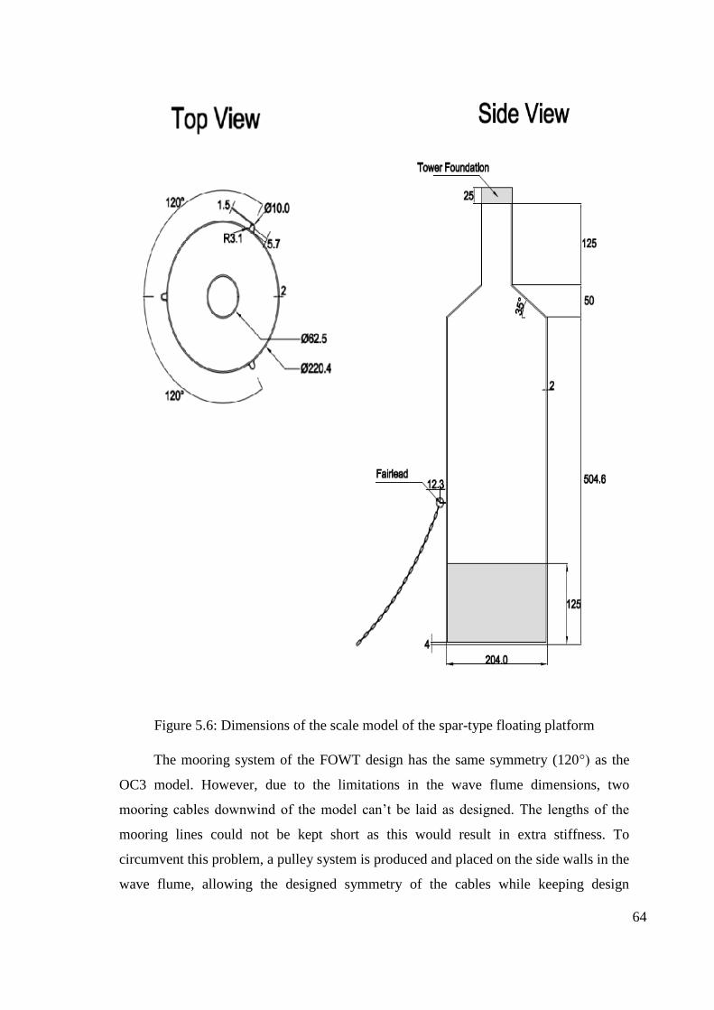
64
Figure 5.6: Dimensions of the scale model of the spar-type floating platform
The mooring system of the FOWT design has the same symmetry (120°) as the
OC3 model. However, due to the limitations in the wave flume dimensions, two
mooring cables downwind of the model can’t be laid as designed. The lengths of the
mooring lines could not be kept short as this would result in extra stiffness. To
circumvent this problem, a pulley system is produced and placed on the side walls in the
wave flume, allowing the designed symmetry of the cables while keeping design

65
parameters and the stretching-loosening ability of the mooring lines intact. The pulley
system is shown in Figure 5.7.
Figure 5.7: Pulley system for the leeward mooring lines
The experimental model setup is an ongoing process. Currently, the wave
measurement system is fully implemented and functional (see. Section 5.3), and both
regular and irregular waves can be generated and measured in the wave channel. The
devices to measure the tension forces on the mooring cable and to capture the motion
responses of the spar-type floating offshore wind turbine under regular and irregular
waves are not implemented yet and planned for the near future.

66
A top-down sketch of the wave flume setup is given in Figure 5.8:
Figure 5.8: Top-view sketch of the wave flume

67
5.3. Wave Measurement and Analysis
As explained in Chapter 4, Using the wavemaker theory, a code is written to
produce the wave signal for the wave generator. Therefore, it is possible to generate
regular or irregular random wave series in the laboratory wave flume (see Section 4.3).
To use the waves produced by the piston-type wave generator, wave measurements
need be to taken and compared with the waves that were generated theoretically.
Waves are measured using the HR Wallingford Wave Measurement System™
which consists of 60 cm twin wire analog wave probes and a wave gauge monitoring
device with a built-in 16 bit A/D converter. The wave probes can be described as a steel
wire that acts as a resistor when submerged in water. While the wave probes operate,
the current that flows between the wires is converted to the output voltage and logged in
the wave gauge monitor. If the probes are submerged further, or the probes encounter
the wave crest, the resistance will shorten, producing an increase in the output voltage,
vice versa.
The data logged in the wave gauge monitor are analyzed in Python using the code
that is written in house. Wave probes are mounted on wooden planks to make the re-
location practical. Images of the mounted wave probes and the wave gauge monitor are
shown in Figure 5.9 and Figure 5.10, respectively.
The analog readings measured by the wave probes are transferred to the wave
gauge system in the observation room. The wave gauge measurement system converts
the analog reading to digital data using a built-in 16-bit A/D converter. The digital
output is then converted to wave heights in cm unit using the transfer functions derived
from calibration.
The wave gauge measurement system has an output voltage between -10V and
+10V. The voltage data is read on the data acquisition software and can be logged in the
computer that is connected to the wave gauge measurement system. The voltage data
that is logged is read using a Python code written in-house. The voltage readings can be
converted to water surface profile measurements in length units using the conversion
equations obtained by the calibration of the wave probes.

68
Figure 5.9: Wave probes, mounted on the wave flume
Figure 5.10: Wave gauge monitor

69
5.3.1. Calibration & Measurement
To convert the voltage differences to the water surface profile, calibration
should be done daily before the start of the experiment. The calibration scheme is as
follows (HR Wallingford, 2015):
-After the probes are placed at the designated locations, analog gain for every
probe is changed so that it shows 0 in still water level.
-The expected maximum wave height is considered and the calibration range is
set to higher bounds to catch the trough and crest of the maximum wave
-Voltage data are read for each probe at still water level and recorded
-Measurement range is divided into steps
-Starting from SWL, probes are moved downwards in pre-designated steps, for
each step, voltage readings are noted
-When the maximum depth range is reached, probes are moved upwards in pre-
designated steps and voltage readings are noted for each step
-At the point of minimum depth for the probes, the same procedure is repeated
downwards until the wave probe reached its initial position in SWL
-Recorded voltages are plotted and formulas that convert the probe voltage to
wave height for each wave gauge are obtained using linear regression.
An example for the calibration of a wave probe is given in Table 5.4 and Figure
5.11, readings are taken at SWL for -12, -6, 0, 6, 12 cm depths:
Table 5.4: Wave probe calibration example
Wave probe voltage reading (V) Submerged depth of the probe
from the reference point (cm)
0.003 0
2.171 6
4.367 12
(cont. on next page)

70
Table 5.4 (cont.)
2.164 6
-0.004 0
-2.088 -6
-4.125 -12
-2.095 -6
-0.003 0
Figure 5.11: Linear regression to obtain the depth-voltage relationship
Conversion formulas are obtained after performing calibration for each probe. In
the experiments, the measurements taken are logged into a text file using the built-in
software of the wave gauge monitor, which are then analyzed using the code written in
Python for this purpose.
An example of an irregular wave measurement taken in the wave flume is given
with spectral properties, 𝐻𝑠 = 12.5 𝑐𝑚, and 𝑇𝑝 = 1.5 𝑠. After obtaining the irregular
wave time series and the piston displacement matrix, the data is converted to the driving
signal for the wave generator. After waiting a sufficient time for the first re-reflected
waves from the wave board to reach the wave probe, measurements are taken for at least
a hundred wave periods as described in Goda (2000), the voltage data is logged to a text
file and analyzed in the Python code. The first sixty seconds of the irregular wave

71
measurement is given in Figure 5.12. The zero-up crossing yields 𝐻𝑠 = 12.46 𝑐𝑚 and
𝑇𝑠 = 1.60 𝑠. The wave parameters are found to be quite close to the targeted
characteristics.
Figure 5.12: Irregular wave measurement taken in the wave flume
5.4. Passive Absorption of the Reflected Waves
A well-known problem in physical experiments in wave flumes is the reflection.
The waves propagating forward reflect off the wall at the end of the flume, then return
to the wave board and reflect off towards the forward end of the channel again, until the
wave energy dissipates completely. The reflections and re-reflections can distort the
wave record and result in inconsistencies in the experiments. One way to circumvent
this problem is the burst method (Madsen 1970) where a burst of waves is generated
and measured until the reflections become effective in the wave record. The first few
waves of the burst waves will also be removed from the record due to the wave board
starting its motion from rest producing larger waves. In this study, this method is used
in the initial tests of the regular wave generating capabilities of the wave generator.

72
However, the load cases for the FOWT model requires wave trains to be generated on
much longer time periods. Therefore, a dissipating beach consisting of rocks of varying
sizes is laid at the end of the channel with a 1/5 slope to mitigate the reflections
occurring in the wave flume. The dissipating beach is shown in Figure 5.13.
Figure 5.13: Dissipating beach
In addition to the reflection problem at the end of the channel, there is a similar
problem at the beginning of the channel at the back of the generator. Since the water is
present at both sides of the wave board, waves propagate to the backward of the board
and create splashes of water that cause risks of damaging the motor when the generated
and reflected waves overlap. Thus, a steel cage filled with an absorbing material (plastic
sponges) is placed at the back of the generator to absorb the wave energy there. (see
Figure 5.14). It is observed that the plastic sponge material absorbs much of the wave
energy and eliminates the risk of damaging the motor.
A much better way to deal with reflection would be achieved by the active
absorption of the reflected waves. In active absorption systems, the reflected waves are

73
absorbed by a device that is similar to the wave board that produces progressive waves
in the wave flume. Placed at the reflecting end of the flume, this device should force the
incoming waves in a way that absorbs them, instead of reflecting them (Dean and
Dalrymple 1984). However, considering the dissipating beach laid at the end of the
flume, there is no room for such a system.
Figure 5.14: The wave absorbing steel cage
Another approach to active absorption is “the absorbing wave board” which lets
the wave generator perform the absorbing motion whenever the reflected waves arrive.
To implement this method, real-time force measurements on the wave board using force
transducers (Hughes 1993) or real-time water surface elevation near the board (Schaffer
and Jakobsen 2003) is necessary. Either way, to implement such a system, an active
feedback control system needs to be established. The implementation of active
absorption capabilities is aimed at the piston-type wave generator in the future.

74
CHAPTER 6
CONCLUSIONS
A numerical model is investigated to gain inference on the dynamic response of a
spar-type floating offshore wind turbine under regular and irregular wave loads.
Floating spar-type platform supporting a 5-MW baseline wind turbine and the catenary
mooring lines that anchor the structure to the seabed is modeled, taking the
specifications provided in OC3 Phase IV code collaboration comparison. Wind loads
and servo-elastic behavior of the FOWT is kept out of scope. The obtained results show
agreement with the other participants’ results in OC3. Investigation of the system
response under wave loads provided valuable information regarding the stability
performance of the spar model. It is inferred from the results that the spar model
performs best in heave DOF, staying virtually unaffected from the wind loads.
However, surge and pitch responses of the model showed that the model is indeed quite
vulnerable to wave loads in these degrees of freedom, so, the natural frequencies in
pitch and surge should best be away from the peak frequency of the wave spectrum.
Aiming to prepare the laboratory wave environment necessary to conduct
physical model experiments in the wave flume located in the hydraulics laboratory in
IZTECH, efforts are made in the production of a wave generator with regular and
irregular wave generation capabilities. The investigation of the established wavemaker
theory revealed that the correct reproduction of naturally occurring waves is not
possible using the first-order solutions of velocity potential in the boundary value
problems at the wavemaker. In fact, due to the assumptions at the wave board, first-
order wave board motion produces spurious waves at low frequency and high-frequency
regions of the spectrum, termed subharmonics and superharmonics, respectively. The
second-order corrections for both regular and irregular waves are investigated and
transfer functions are provided in this study, with the inclusion of an iFFT method used
to apply the corrections to the wavemaker code written for the laboratory wave
generator. As of the writing of this thesis, second-order regular wave generation is fully
implemented in the piston-type wave generator in the wave flume, and while the
second-order irregular wave generator code is completed, it is not encoded in the wave
75
generator and tested yet. However, by taking into consideration the results obtained in
the numerical investigation of the OC3 spar model, which revealed that the natural
frequencies of the floating structure lie in the low-frequency region, it is possible to
deduce that the second-order effects, especially subharmonic waves will influence the
motion response of the floating platforms considerably and the elimination of the
spurious harmonic waves is of utmost importance.
The wave flume is prepared for testing the waves generated by the piston-type wave
generator located in the flume. The theoretically generated waves are transformed into
the wave board position matrix in the time domain that is required to create the targeted
wave series. The position matrix is then converted to the driving signal for the AC servo
motor which oscillates the wave board. The conversion of the wave board position to
the motor signal is out of scope for this thesis. However, an integrated graphical user
interface is created and used to run the codes generating the position matrix and the
driving signal. To measure the waves, a wave gauge system which consists of analog
wave probes and a wave gauge monitor with a 16-bit A/D converter is used. The
implementation of the wave generation and measurement part of the laboratory setup is
complete and second-order regular and first-order irregular waves are tested.
A very common problem in laboratory wave generation is wave reflection. To
mitigate the reflection waves in the wave flume, an energy-dissipating beach consisting
of small-sized rocks are laid at the end of the channel at a 1:5 slope and substantial
improvements are observed in the generated waves. Then, a reflection analysis is
conducted using irregular wave measurements. The results revealed that the reflection is
still influential in the wave flume although reflected waves occupying a smaller
percentage of the total wave energy. For future works in this project, the active
absorption method is aimed to be implemented in wave generation. However, the first
challenge in the active absorption will be the implementation of an active feedback
system between the real-time wave measurements and the driving signal that is sent to
the AC motor of the wave generator.
The Froude scaling is applied to obtain the model of a spar-type floating platform.
The dynamic similitude is achieved and the floating platform model and catenary
mooring lines are constructed with properties derived from a 1:40 length scale. To
retain the original symmetry of the mooring lines requires the tests to be conducted in a
76
large basin. However, the dimensions of the laboratory wave flume introduce
limitations in the lateral axis. Thus, a compromise has been made to keep the original
symmetry of the mooring lines at the platform location; a pulley system that lets the
mooring cables traverse through is designed and produced. The pulleys, when mounted
on the sidewalls of the wave flume close to the spar model, allows the mooring lines to
retain their original symmetries from the spar model to the pulleys, the rest of the
mooring line sections pass through the pulleys, and their direction changes to parallel to
the longitude of the wave flume. For practical reasons, the pulleys are mounted on the
sidewalls using industrial stainless magnets, which allows easier relocation when
needed. Adopting this layout allows the mooring lines to tighten and loosen, according
to the motion of the floating platform while preserving the original mooring line
properties, yet, some energy loss due to friction is expected as the lines traverse through
the pulleys. However, at this point, the measurement instruments for the cable tensions
and platform time response are not implemented. As a future study, experiments will be
conducted to measure the responses of the FOWT under various regular and irregular
waves and results will be used to verify the numerical model study performed in this
thesis.

77
REFERENCES
Alkarem, Yüksel. 2020. “Numerical Examination of Floating Offshore Wind Turbine
and Development of an Innovative Floating Platform Design.”
Aqwa, Ansys. 2013. “Introduction to Hydrodynamic Analysis with Ansys Aqwa.”
Aqwa, 1–32.
Barthel, V., E. P.D. Mansard, S. E. Sand, and F. C. Vis. 1983. “Group Bounded Long
Waves in Physical Models.” Ocean Engineering 10 (4): 261–94.
https://doi.org/10.1016/0029-8018(83)90012-4.
Biesel, F. 1951. “Etude Théorique d’un Certain Type d’appareil a Houle.” La Houille
Blanche 2 (4): 475–96.
BNEF. 2018. “Global Offshore Wind Market Set to Grow Sixfold by 2030.” January 8.
2018. https://about.bnef.com/blog/global-offshore-wind-market-set-to-grow-
sixfold-by-2030/.
Bouws, E., H. Gunther, W. Rosenthal, and C. L. Vincent. 1985. “Similarity of the Wind
Wave Spectrum in Finite Depth Water 1. Spectral Form.” Journal of Geophysical
Research 90 (C1): 975–86. https://doi.org/10.1029/JC090iC01p00975.
Bretschneider, C. L. 1959. Wave Variability and Wave Spectra for Wind-Generated
Gravity Waves. No. 118. The Board.
Butterfield, Sandy, W Musial, Jason Jonkman, and Paul Sclavounos. 2005.
“Engineering Challenges for Floating Offshore Wind Turbines.” Offshore Wind
Conference, 13.
Chakrabarti, Subrata. 1995. “Offshore Structure Modelling.” Applied Ocean Research
17 (6): 391–92. https://doi.org/10.1016/s0141-1187(96)00012-0.
Dean, R. G., and R. A. Dalrymple. 1984. Water Wave Mechanics for Engineers and
Scientists. https://doi.org/10.1029/eo066i024p00490-06.
Erol, Serkan. 2020. “SCALED DOWN MODELLING OF A HORIZONTAL WIND
TURBINE FOR A FLOATING WIND TURBINE RESEARCH.”

78
Flick, Reinhard E., and Robert T. Guza. 1980. “Paddle Generated Waves in Laboratory
Channels.” Journal of the Waterway, Port, Coastal and Ocean Division,
Proceedings of the American Society of Civil Engineers 106 (1): 79–97.
Fontanet, Pierre. 1961. “Théorie de La Génération de La Houle Cylindrique Par Un
Batteur Plan (2e Ordre d’approximation).” Houille Blanche, no. 1: 3–31.
https://doi.org/10.1051/lhb/1961020.
Funke, E.R, E.P.D. Mansard, and G. Dai. 1988. “REALIZABLE WAVE
PARAMETERS IN A LABORATORY FLUME.” In 21st International
Conference on Coastal Engineering, 835–48.
Gilbert, G., D. M. Thompson, and A. J. Brewer. 1971. Design Curves for Regular and
Random Wave Generators. Journal of Hydraulic Research. Vol. 9.
https://doi.org/10.1080/00221687109500345.
Goda., Yoshimi, and Yasumasa Suzuki. 1976. “Estimation of Incident and Reflected
Waves in Random Wave Experiments.” Ocean Engineering 22 (1): 77–86.
https://doi.org/10.1016/0029-8018(93)E0011-G.
Goda, Yoshimi. 1967. “Travelling Secondary Wave Crests in Wave Channels.”
———. 1970. “Numerical Experiments on Wave Statistics with Spectral Simulation.”
Report Port Harbour Res. Inst. 9: 3–57. http://ci.nii.ac.jp/naid/10011190974/en/.
———. 1979. “A Review on Statistical Interpretation of Wave Data.” Report of the
Port and Harbour Research Institute.
———. 1988. “Statistical Variability of Sea State Parameters as a Function of Wave
Spectrum.” Coastal Engineering in Japan 31 (1): 39–52.
https://doi.org/10.1080/05785634.1988.11924482.
———. 1999. “A Comparative Review on the Functional Forms of Directional Wave
Spectrum.” Coastal Engineering Journal 41 (1–4): 1–20.
https://doi.org/10.1142/s0578563499000024.
———. 2000. Random Seas and Design of Maritime Structures. World Scientific. Vol.
15.
GWEC. 2019. “Global Wind Report 2019.” 2019. https://gwec.net/global-wind-report/

79
Hasselmann, K. 1973. “Measurements of Wind-Wave Growth and Swell Decay during
the Joint North Sea Wave Project (JONSWAP).” Deutches Hydrographisches
Institut, no. Ergänzungsheft 8-12.
Havelock, T H. 1929. “LIX . Forced Surface-Waves on Water.” The London,
Edinburgh, and Dublin Philosophical Magazine and Journal of Science 8 (51):
569–76. https://doi.org/10.1080/14786441008564913.
Huang, Norden E., Steven R. Long, Chi Chao Tung, Yeli Yuen, and Larry F. Bliven.
1981. “A Unified Two-Parameter Wave Spectral Model for a General Sea State.”
Journal of Fluid Mechanics 112 (55): 203–24.
https://doi.org/10.1017/S0022112081000360.
Hughes, Steven A. 1993. Physical Models and Laboratory Techniques in Coastal
Engineering. Advanced Series on Ocean Engineering. Vol. Volume 7. WORLD
SCIENTIFIC. https://doi.org/doi:10.1142/2154.
Hyun, Jae Min. 1976. “Simplified Analysis of a Plunger-Type Wavemaker
Performance.” Journal of Hydronautics 10 (3): 89–94.
https://doi.org/10.2514/3.63056.
Jonkman, J. 2010. “Definition of the Floating System for Phase IV of OC3.” Contract 1
(May): 31. https://doi.org/10.2172/979456.
Jonkman, J, and W Musial. 2010. “Offshore Code Comparison Collaboration (OC3) for
IEA Task 23 Offshore Wind Technology and Deployment.” IEA Task 23 303
(December): 74. https://doi.org/NREL/TP-5000-48191.
Landberg, Lars. 2016. Meteorology for Wind Energy.
https://doi.org/10.1002/9781118913451.
Mackay, E. B.L. 2012. Resource Assessment for Wave Energy. Comprehensive
Renewable Energy. Vol. 8. Elsevier Ltd. https://doi.org/10.1016/B978-0-08-
087872-0.00803-9.
Madsen, O. S. 1970. “Waves Generated by a Piston-Type Wavemaker.” Coastal
Engineering, 589–607. https://doi.org/10.31826/9781463231699-040.
Madsen, O.S. 1971. “On the Generation of Long Waves.” Coastal Engineering 76 (36).

80
https://doi.org/10.1029/JC076i036p08672
Mansard, E. P.D. 1988. “Sub and Superharmonics in Natural Waves.” Journal of
Offshore Mechanics and Arctic Engineering 110 (3): 210–17.
https://doi.org/10.1115/1.3257053.
Martin, Heather R., Richard W. Kimball, Anthony M. Viselli, and Andrew J. Goupee.
2014a. “Methodology for Wind/Wave Basin Testing of Floating Offshore Wind
Turbines.” Journal of Offshore Mechanics and Arctic Engineering 136 (2):
021902. https://doi.org/10.1115/1.4025030.
———. 2014b. “Methodology for Wind/Wave Basin Testing of Floating Offshore
Wind Turbines.” Journal of Offshore Mechanics and Arctic Engineering 136 (2):
020905. https://doi.org/10.1115/1.4025030.
Miles, M. D., and E. P. Funke. 1988. “NUMERICAL COMPARISON OF WAVE
SYNTHESIS METHODS.” In 21st International Conference on Coastal
Engineering. https://ascelibrary.org/doi/pdf/10.1061/9780872626874.007.
———. 1989. “A Comparison of Methods for Synthesis of Directional Seas.” Journal
of Offshore Mechanics and Arctic Engineering 111 (1): 43–48.
https://doi.org/10.1115/1.3257137.
Mitsuyasu, H. 1970. “On the Growth of Wind-Generated Waves (2)-Spectral Shape of
Wind Waves at Finite Fetch-.” Proc. 17th Japanese Conf. Coastal Eng., 1970.
http://ci.nii.ac.jp/naid/10018957596/en/.
Newland, D. E. 2012. An Introduction to Random Vibrations, Spectral & Wavelet
Analysis. Courier Corporation.
Newman, J. N. 1990. “Numerical Solutions of the Water-Wave Dispersion Relation.”
Applied Ocean Research 12 (1): 14–18. https://doi.org/10.1016/S0141-
1187(05)80013-6.
Ottesen-Hansen, N. E. 1978. “Long Period Waves in Natural Wave Trains.”
Ottesen-Hansen, N. E., Stig E Sand, H. Lundgren, Torben Sorensen, and H. Gravesen.
1980. “CORRECT REPRODUCTION OF GROUP-INDUCED LONG WAVES.”
In Coastal Engineering 1980, 784–800.

81
Pierson, Willard J., and Lionel Moskowitz. 1964. “A Proposed Spectral Form for Fully
Developed Wind Seas Based on the Similarity Theory of S. A. Kitaigorodskii.”
Journal of Geophysical Research 69 (24): 5181–90.
https://doi.org/10.1029/jz069i024p05181.
Samii, K., and J. K. Vandiver. 1984. “A Numerically Efficient Technique for the
Simulation of Random Wave Forces on Offshore Structures.” Proceedings of the
Annual Offshore Technology Conference 1984–May: 301–8.
https://www.onepetro.org/conference-paper/OTC-4811-MS.
Sand, Stig E. 1982a. “Long Wave Problems in Laboratory Models.” Journal of the
Waterway, Port, Coastal and Ocean Division 108 (4): 492-503.
———. 1982b. “Long Waves in Directional Seas.” Coastal Engineering 6 (3).
https://doi.org/10.1016/0378-3839(82)90018-7.
Sand, Stig E., and Bjarne Donslund. 1985. “Influence of Wave Board Type on Bounded
Long Waves.” Journal of Hydraulic Research 23 (2): 147–63.
https://doi.org/10.1080/00221688509499362.
Sand, Stig E., and E. P.D. Mansard. 1986. “Reproduction of Higher Harmonics in
Irregular Waves.” Ocean Engineering 13 (1): 57–83. https://doi.org/10.1016/0029-
8018(86)90004-1.
Schaffer, H. a., and K. P. Jakobsen. 2003. “Non-Linear Wave Generation and Active
Absorption in Wave Flumes.” Long Waves Symposium, no. January 2003: 69–76.
Schäffer, Hemming A. 1994. “Second Order Irregular-Wave Generation in Flumes -
Computation of Transfer Functions by an Asymptotic Summation Method.” In ,
784–97.
———. 1996. “Second-Order Wavemaker Theory for Irregular Waves.” Ocean
Engineering 23 (1): 47–88. https://doi.org/10.1016/0029-8018(95)00013-B.
Schäffer, Hemming A., and Cathrine M Steenberg. 2003. “SECOND-ORDER WAVE
GENERATION IN LABORATORY BASSINS.” Ocean Engineering 30 (10):
1203–31.
Snyder, Brian, and Mark J. Kaiser. 2009. “Ecological and Economic Cost-Benefit

82
Analysis of Offshore Wind Energy.” Renewable Energy 34 (6): 1567–78.
https://doi.org/10.1016/j.renene.2008.11.015.
Spinneken, Johannes, and Chris Swan. 2009a. “Second-Order Wave Maker Theory
Using Force-Feedback Control. Part I: A New Theory for Regular Wave
Generation.” Ocean Engineering 36 (8): 539–48.
https://doi.org/10.1016/j.oceaneng.2009.01.019.
———. 2009b. “Second-Order Wave Maker Theory Using Force-Feedback Control.
Part II: An Experimental Verification of Regular Wave Generation.” Ocean
Engineering 36 (8): 549–55.
Stokes, G. G. 1880. “On the Theory of Oscillatory Waves.” Transactions of the
Cambridge Philosophical Society. http://ci.nii.ac.jp/naid/10010286911/en/.
Sulisz, W., and R. T. Hudspeth. 1993. “Complete Second-Order Solution for Water
Waves Generated in Wave Flumes.” Journal of Fluids and Structures.
https://doi.org/10.1006/jfls.1993.1016.
Tuah, Hang, and Robert T. Hudspeth. 1982. “Comparisons of Numerical Random Sea
Simulations.” Journal of the Waterway, Port, Coastal and Ocean Division 108 (4):
569–84. https://cedb.asce.org/CEDBsearch/record.jsp?dockey=0034804.
Ursell, F., R. G. Dean, and Y. S. Yu. 1960. “Forced Small-Amplitude Water Waves: A
Comparison of Theory and Experiment.” Journal of Fluid Mechanics 7 (1): 33–52.
https://doi.org/10.1017/S0022112060000037.
Wallingford, H. R. 2015. Wave Gauge System User Manual.
Wang, H. T., and J. D. Crouch. 1993. “Accuracy of Low‐Order Models for Simulations
of Random Ocean Waves.” Journal of Waterway, Port, Coastal, and Ocean
Engineering 119 (1): 70–87. https://doi.org/https://doi.org/10.1061/(ASCE)0733-
950X(1993)119:1(70).
Wang, Shen. 1974. Plunger-Type Wavemakers: Theory And Experiment. Journal of
Hydraulic Research. Vol. 12. https://doi.org/10.1080/00221687409499732.
Wu, Yung Chao. 1988. “Plunger-Type Wavemaker Theory.” Journal of Hydraulic
Research 26 (4): 483–91. https://doi.org/10.1080/00221688809499206.