water

Article

Watershed Sediment and Its Effect on StorageCapacity: Case Study of Dokan Dam Reservoir

Mohammad Ezz-Aldeen 1, Rebwar Hassan 1, Ammar Ali 2, Nadhir Al-Ansari 1,* ID andSven Knutsson 1

1 Department of Civil, Environmental and Natural Resources Engineering, Lulea University of Technology,971 87 Lulea, Sweden; mohezz@ltu.se (M.E.-A.); rebwar.hassan@ltu.se (R.H.); Sven.Knutsson@ltu.se (S.K.)

2 Department of Water Resources Engineering, Baghdad University, Baghdad 10071, Iraq;ammali_75@yahoo.com

* Correspondence: nadhir.alansari@ltu.se; Tel.: +46-920-491-858

Received: 28 May 2018; Accepted: 26 June 2018; Published: 28 June 2018�����������������

Abstract: Dokan is a multipurpose dam located on the Lesser Zab River in the Iraq/Kurdistan region.The dam has operated since 1959, and it drains an area of 11,690 km2. All reservoirs in the world sufferfrom sediment deposition. It is one of the main problems for reservoir life sustainability. Sustainablereservoir sediment-management practices enable the reservoir to function for a longer period of timeby reducing reservoir sedimentation. This study aims to assess the annual runoff and sediment loadsof the Dokan Dam watershed using the soil and water assessment tool (SWAT) model to evaluatethe relative contributions in comparison with the total values delivered from both watershed andLesser Zab River and to identify the basins with a high sediment load per unit area. These help in theprocess of developing a plan and strategy to manage sediment inflow and deposition. The SUFI-2program was applied for a model calibrated based on the available field measurements of the adjacentDerbendekhan Dam watershed, which has similar geological formations, characteristics and weather.For the calibration period (1961–1968), the considered statistical criteria of determination coefficientsand Nash–Sutcliffe model efficiency were 0.75 and 0.64 for runoff while the coefficients were 0.65and 0.63 for sediment load, respectively. The regionalization technique for parameter transformationfrom Derbendekhan to Dokan watershed was applied. Furthermore, the model was validated basedon transformed parameters and the available observed flow at the Dokan watershed for the period(1961–1964); they gave reasonable results for the determination coefficients and Nash–Sutcliffe modelefficiency, which were 0.68 and 0.64, respectively. The results of SWAT project simulation for Dokanwatershed for the period (1959–2014) indicated that the average annual runoff volume which enteredthe reservoir was about 2100 million cubic meters (MCM). The total sediment delivered to thereservoir was about 72 MCM over the 56 years of dam life, which is equivalent to 10% of the reservoirdead storage. Two regression formulas were presented to correlate the annual runoff volume andsediment load with annual rain depth for the studied area. In addition, a spatial distribution ofaverage annual sediment load was constructed to identify the sub basin of the high contribution ofsediment load.

Keywords: Dokan Dam; runoff; sediment load; SWAT

1. Introduction

Most of the dams, storage schemes, and different hydraulic structures around the world sufferfrom sedimentation problems. For dams and reservoirs, this effect is mainly concerned with the designcapacity and operation schedule. The main source of reservoir sediments is the main river flow in

Water 2018, 10, 858; doi:10.3390/w10070858 www.mdpi.com/journal/water

Water 2018, 10, 858 2 of 16

addition to the runoff water, carrying the sediment load from watersheds and valleys surroundingthe reservoir.

After a long period of dam operation, it is usually necessary to evaluate the current storagecapacity of the reservoir relative to that in the design stage. The runoff and sediment load delivered tothe reservoir could be estimated based on measured values of continuous river flow. Schleiss et al. [1]highlights and discusses the main matters concerning reservoir sedimentation. The reservoirsedimentation problem should be considered from the early stages of planning design and operation.In addition, the sedimentation process can create problems downstream from the dam which shouldalso be considered in the planning and design stages.

Physically based models are usually used in cases where runoff and sediment load data recordsare not available. These models are of two types, which are referred to as single storm modelsand continuous simulation models. The Areal Non-Point Source Watershed Environment ResponseSimulation (ANSWERS) is developed by Beasley et al. [2]; and the European Soil Erosion Model(EUROSEM) was improved by Morgan et al. [3]; all of those models mentioned are examplesof the former models. Examples of the latter are the spatially distributed erosion and sedimentyield component, chemicals, runoff and erosion from agricultural management systems CREAMS(Science and Education Administration; Department of Agriculture, Washington, WA, USA) whichare proposed by Knisel [4]; the SHESED model (the hydrologic and sediment transportation modelof hydrological modeling system (SHE)) which is proposed by Wicks and Bathurst [5]; and the soiland water assessment model (SWAT) that was developed by Arnold et al. [6]. The SWAT model isthe most commonly used model and, for this reason, a number of researchers have modified thismodel for different purposes (see [7,8]). Durao et al. [9] estimates the transported nutrient load in theArdila River watershed in Spain by applying the SWAT model in order to identify the contributionof this load to the whole watershed. The model is applied to simulate long-period data; the realdaily precipitation data is considered for the period 1930–2000. The considered flow data for modelcalibration and validation extend from 1950 to 2000, and nutrient data stretch from 1981 to 1999.The results indicate that the main source of diffusion prolusion comes from the main tributaries ofSpain. Wang et al. [10] tests the possible conservation practices within a rangeland watershed usingthe agricultural policy/environmental extender (APEX). The model is calibrated and validated forboth flow and sediment yield for the Cowhouse Creek watershed in north Texas. The analysis of thescenario extends from 1951 to 2008. It shows that a significant reduction reaches to 58.8% of overlandsediment losses from the area covered by a range brush to range grass. This reduction is due to thereplacement of shrub species with herbaceous species within the subareas. Samaras and Koutitas [11]evaluates the effect of land-use changes in a watershed on coastal erosion for a selected area in northGreece. They apply both the SWAT model and a shoreline evolution model, a shoreline evolutionmodel, for this purpose. The simulation is applied before and after land use change using threeformulas of sediment transportation. The result indicates that a reduction in crop/land use cover from23.3% to 5.1% leads to a reduction in both watershed sediment yield and sediment discharge at theoutlet by (56.4%) and (26.4 to 12.8%), respectively. This study can be considered as a suitable tool andguide for future work in the same field. Samaras and Koutitas [12] studies the effect of climate changeon sediment transport and morphology. The study is applied to a selected sandy coast area and itswatershed in North Greece. Both SWAT models are implemented for the watershed and PELNCON-Mis implemented for the coastal area to achieve the study aims. Two scenarios are employed; the firstone is considered to be an extreme rise in the precipitation depth on the watershed, and the secondone is considered to be an extreme rise in waves in the coastal area. Results of the first scenario showsa significant effect on erosion, sediment transport, sediment yield and discharge at the watershedoutlet, while the second scenario indicates a lower effect on the coastline variation. Arnold [13]developed the SWAT + CUP model ( SWAT Calibration and Uncertainty Programs, Swiss FederalInstitute of Aquatic Science and Technology, Zurich, Switzerland), which provides a semi-automatictool for decision-making for the SWAT model by applying both manual and automated calibration

Water 2018, 10, 858 3 of 16

and incorporating both sensitivity and uncertainty analysis. A number of previous studies [14–17]were applied using the SWAT model to estimate runoff, sediment yield and/or other soluble materialsfor ungagged watersheds based on neighboring or similar property watersheds. Another technique isused for flow and erosion, and sediment transport is the distributed mode. Juez et al. [18] simulatesthe hydro-sedimentary response of the Western Mediterranean catchment to a representative rainfallstorm. The simulation combines the distributed flow surface model with the empirical model forinfiltration, the Soil Conservation Services Model (SCS), and the erosion model, which is the HillslopeErosion Model (HEM), considering water depth and flow as a 2D model. The present model is a toolfor analyzing the hydro-sedimentary process at a temporal and special scale.

Most countries in the Middle East suffer from water shortage problems, where the annualallocation per capita does not exceed 500 m3 [19]. For this reason, water is essential to life,socioeconomic development, and political stability in this region. Future prospects are negative;therefore, this problem is expected to be more chronic and severe in future [20]. Iraq used to beconsidered to be a relatively rich country in terms of its water resources, until the mid-1970s, becauseof the presence of the Tigris and Euphrates Rivers [21]. Due to regional and internal problems in Iraq,the estimation of the overall water required is about 75–81 billion cubic meters (BCM) [22], while theavailable quantity is 59–75 BCM and will drop to 17.61 BCM in 2025 [23]. In view of this situation, it isvery important to know the actual storage capacity of the reservoirs—which are unknown now—sothat prudent water resources planning can be done. The sedimentation rate of several reservoirs wasrecently investigated in Mosul and Dohuk. This is the third reservoir to be dealt with in Iraq. The bedof the Dokan Dam reservoir (located in the northeast of Iraq) is surveyed by Hassan et al. [24], and thisstudied the bed sediment using 32-bed samples distributed spatially over the reservoir. The resultsindicate that the bed sediments of the reservoir are composed of silt (48%), clay (23%), gravel (15%)and sand (14%).

All reservoirs in the world suffer from sediment deposition. This is one of the main problems forreservoir life sustainability. Sustainable reservoir sediment-management practices enable continuedreservoir functioning for a longer period by reducing reservoir sedimentation. Iraq suffers from watershortage problems, especially after the construction of a series of storage reservoirs in source countries(Turkey, Syria and Iran), so the evaluation of the actual live storage capacity of dams is importantfor the prudent management of the operation schedule. The aim of this study is to assess the annualrunoff and sediment loads of the Dokan Dam watershed (ungagged area) using a SWAT model set-upbased on the parameter transformation technique of the modeling-gauged Derbendekhan watershedto learn the hydrological behavior of the area and to assess its contribution to the total values pouringinto the reservoir. Moreover, the set-up model helps us to find the spatial distribution of erosion andannual sediment yield for the sub basins. This will help us to find the sub basins with a high sedimentyield and evaluate effective factors for them. These assessments help in the process of developing aplan and a strategy for managing the sediment inflow and deposition.

2. Study Area

2.1. Location and Topography

The considered study area is the watershed of the Dokan Dam reservoir, situated in the northeastof Iraq (Figure 1). Dokan dam is a concrete arch dam located in the Lower Zab River, about 65 kmsoutheast of Sulaimaniyah city and 295 km north of Baghdad, the capital city of Iraq. The dam heightis about 116 m at maximum river depth, having a total storage capacity of 6.87 × 109 m3 (6.14 × 109 m3

live storage and 0.73 × 109 m3 dead storage) at normal operation level of 511 m.a.s.l. [22]. The damhas been built to serve irrigation, power generation, water supply and flood control needs. Due to thelimited observed data of flow at the Dokan Dam watershed and the unavailability of sediments loaddata, the second watershed considered for this research is the Derbendekhan Dam watershed; it is thenearest watershed to the study area. The properties of the Dokan and Derbendikhan watersheds are

Water 2018, 10, 858 4 of 16

shown in Table 1. The digital elevation model (DEM) with 30 m resolution is considered to identify thewatershed boundary, classification of overland and channel flow, slopes and other properties.

Water 2018, 10, x FOR PEER REVIEW    4 of 16 

Table 1. Properties of the Dokan and Derbendekhan watersheds. 

Watershed Area 

(km2) 

Max. 

Elevation 

(m.a.s.l) 

Min. 

Elevation 

(m.a.s.l) 

Average 

Slope (%) 

Maximum 

Annual Rain 

(mm) 

Minimum 

Annual Rain 

(mm) 

Dokan Dam  11,690  3557  489  26.5  1125  182 

Derbendekhan 

Dam 15,280  3332  375  23.3  970  174 

 

Figure 1. Topographic map of the watershed areas of the Dokan and Derbendekhan Dams and their 

locations in Iraq. 

2.2. Soil Type and Land Use 

The exposed rocks at the Dokan and Derbendekhan watershed areas are mainly limestone and 

minor exposures of dolomitic limestone, dolomite, and Quaternary alluvial deposits [25,26]. Based 

on  the Reconnaissance Soil Map of  the  three Northern Governorates,  Iraq  [26] and  the Food and 

Agriculture Organization of the United Nations (FAO) soil map [27], both watersheds are located on 

a common extended type of soil classification. Samples for different soil classes were taken depending 

on the soil map of the study area. A map of soil types is prepared for this study as a shape file for 

each watershed  to  be used  in  the  SWAT model  (see  below  for model details). The  soil  samples 

analysis  includes grain  size distribution  in different  types, organic matter  content  and hydraulic 

conductivity. The analysis of soil samples indicates that the area generally consists of four major soil 

types. Most of the area (85.6%) is covered by gravelly sandy mud; 6.9% is gravelly mud; and 7.5% of 

two types of muddy gravel (the main differences between the two types are the percent of gravel, 

which  is 74% and 56%  for  types 1 and 2, respectively). Figure 2 shows  the shape  file of soil  type 

considered in the SWAT model for the Dokan watershed. 

The land use map for the years (1976–1979) [28] and available satellite image (NASA’s Landsat 

GeoCover, 2007, with a spatial resolution of 14.25 m) indicates that the winter plants and pastures 

represent the main part of the land use map of the studied area. This depends on rainfall as a main 

source of irrigation water. The other parts are forests, vegetables and urban areas (villages). The land 

use change is limited (see Table 2). This is mainly due to the geological nature of both watersheds. In 

addition, the topography of the area does not enhance any changes. It is noteworthy to mention that 

rain is the main source of irrigation. For these reasons, the land cover did not change widely through 

the study period since the operation of the dam from the year 1959 to the year 2014. The Dam and 

Figure 1. Topographic map of the watershed areas of the Dokan and Derbendekhan Dams and theirlocations in Iraq.

Table 1. Properties of the Dokan and Derbendekhan watersheds.

Watershed Area(km2)

Max.Elevation(m.a.s.l)

Min.Elevation(m.a.s.l)

AverageSlope (%)

MaximumAnnual

Rain (mm)

MinimumAnnual

Rain (mm)

Dokan Dam 11,690 3557 489 26.5 1125 182Derbendekhan Dam 15,280 3332 375 23.3 970 174

2.2. Soil Type and Land Use

The exposed rocks at the Dokan and Derbendekhan watershed areas are mainly limestoneand minor exposures of dolomitic limestone, dolomite, and Quaternary alluvial deposits [25,26].Based on the Reconnaissance Soil Map of the three Northern Governorates, Iraq [26] and the Food andAgriculture Organization of the United Nations (FAO) soil map [27], both watersheds are located on acommon extended type of soil classification. Samples for different soil classes were taken dependingon the soil map of the study area. A map of soil types is prepared for this study as a shape file foreach watershed to be used in the SWAT model (see below for model details). The soil samples analysisincludes grain size distribution in different types, organic matter content and hydraulic conductivity.The analysis of soil samples indicates that the area generally consists of four major soil types. Most ofthe area (85.6%) is covered by gravelly sandy mud; 6.9% is gravelly mud; and 7.5% of two types ofmuddy gravel (the main differences between the two types are the percent of gravel, which is 74% and56% for types 1 and 2, respectively). Figure 2 shows the shape file of soil type considered in the SWATmodel for the Dokan watershed.

The land use map for the years (1976–1979) [28] and available satellite image (NASA’s LandsatGeoCover, 2007, with a spatial resolution of 14.25 m) indicates that the winter plants and pasturesrepresent the main part of the land use map of the studied area. This depends on rainfall as a mainsource of irrigation water. The other parts are forests, vegetables and urban areas (villages). The landuse change is limited (see Table 2). This is mainly due to the geological nature of both watersheds.In addition, the topography of the area does not enhance any changes. It is noteworthy to mention that

Water 2018, 10, 858 5 of 16

rain is the main source of irrigation. For these reasons, the land cover did not change widely throughthe study period since the operation of the dam from the year 1959 to the year 2014. The Dam and thestudied watershed are located away from the main cities, so changes in the urban and rural areas arelimited. Table 2 shows the percentage of different land use cover for the two periods of the availableland use map.

Water 2018, 10, x FOR PEER REVIEW    5 of 16 

the studied watershed are located away from the main cities, so changes in the urban and rural areas 

are  limited. Table 2  shows  the percentage of different  land use  cover  for  the  two periods of  the 

available land use map. 

 

Figure 2. Soil type classification of the Dokan Reservoir watershed. 

Table 2. Percentages of different land use types for two years of the studied period.   

Year  Winter Plant and Pasture  Forest  Vegetables  Urban Area (Village) 

1976–1979  77.3  22.0  0.5  0.2 

2007  82.7  15.6  1.6  0.1 

Due to the small difference between the percentage of land cover for the two available years, a 

map of land use for the study area is prepared as a shape file (Figure 3). The area consists of four 

types of land use/cover. Winter plants (pasture) and forests of different types of trees cover the main 

part of the study area, while the remaining small area is planted with vegetables near the reservoir 

boundary and/or in urban areas (villages).   

 

Figure 3. Land use and land cover classification of the Dokan Reservoir watershed. 

Figure 2. Soil type classification of the Dokan Reservoir watershed.

Table 2. Percentages of different land use types for two years of the studied period.

Year Winter Plant and Pasture Forest Vegetables Urban Area (Village)

1976–1979 77.3 22.0 0.5 0.22007 82.7 15.6 1.6 0.1

Due to the small difference between the percentage of land cover for the two available years,a map of land use for the study area is prepared as a shape file (Figure 3). The area consists of fourtypes of land use/cover. Winter plants (pasture) and forests of different types of trees cover the mainpart of the study area, while the remaining small area is planted with vegetables near the reservoirboundary and/or in urban areas (villages).

Water 2018, 10, x FOR PEER REVIEW    5 of 16 

the studied watershed are located away from the main cities, so changes in the urban and rural areas 

are  limited. Table 2  shows  the percentage of different  land use  cover  for  the  two periods of  the 

available land use map. 

 

Figure 2. Soil type classification of the Dokan Reservoir watershed. 

Table 2. Percentages of different land use types for two years of the studied period.   

Year  Winter Plant and Pasture  Forest  Vegetables  Urban Area (Village) 

1976–1979  77.3  22.0  0.5  0.2 

2007  82.7  15.6  1.6  0.1 

Due to the small difference between the percentage of land cover for the two available years, a 

map of land use for the study area is prepared as a shape file (Figure 3). The area consists of four 

types of land use/cover. Winter plants (pasture) and forests of different types of trees cover the main 

part of the study area, while the remaining small area is planted with vegetables near the reservoir 

boundary and/or in urban areas (villages).   

 

Figure 3. Land use and land cover classification of the Dokan Reservoir watershed. Figure 3. Land use and land cover classification of the Dokan Reservoir watershed.

Water 2018, 10, 858 6 of 16

3. Applied Model

The soil and water assessment tool (SWAT) is a physically based continuous simulation model forshort or long times that can be applied to large river basins and complex watersheds. It was developedby the US Department of Agriculture, Agricultural Research Service [6]. The model is an efficienttool to estimate the flow and sediment load in addition to different chemical and nutrient materials.The model divides the watershed into sub basins based on their DEM date and hydrological responseunits (HRU); each unit has the same soil type, land use and land slope.

The hydrological simulation is based on the topographical terrain, soil type, land use andhydrological data of daily precipitation, maximum and minimum temperature, wind speed,relative humidity and solar radiation. The flow can be estimated based on a water balance equation;this equation is simulated in the SWAT model by different modular: the land phase and routingphase [14]. For the land phase, the soil water balance calculation is based on the following form [29]:

SWt = SW0 +t

∑i=1

(Rday − Qsur − Ea − wseep − Qqw) (1)

where,

SWt: Water content of the soil (mm);SW0: Initial water content (mm);Rday: Depth of precipitation (mm);Qsur: Equivalent depth of surface runoff (mm);Ea: Evapotranspiration depth (mm);wseep: Depth of water seepage out of considered surface profile (mm);Qqw: Equivalent depth of return flow (mm).

The Penman–Monteith method is considered for potential evapotranspiration estimation.The required input data to estimate the potential evapotranspiration (PET) using the Penman–Monteithmethod are daily solar radiation, air temperature, relative humidity and wind speed. The formula ofthis method considers three effective factors for evapotranspiration, which are the required energy tosustain evaporation, the required strength to remove the water vapor and the aerodynamic in additionto resistance of the surface. The Penman–Monteith method is in the following form [29]:

λE =∆(Hnet − G) + ρair·cp·[eo

z − ez]/ra

∆ + γ·(

1 + rcra

) (2)

where,

λE: Latent heat flux density (MJ/m2/day);E: Evaporation rate (mm/day);∆: Saturation vapor pressure-temperature slope (de/dt) (kPa/Co);Hnet: Net radiation (MJ/m2/day);G: Density of heat flux to the ground (MJ/m2/day);ρair: Density of the air (kg/m3);cp: Specific heat at constant pressure (MJ/kg/day);eo

z: Saturated vapor pressure of air at height z, (kPa);ez: Water vapor pressure of air at height z (kPa);λ: Psychrometric constant (kPa/Co);rc: Resistance of plant canopy (s/m);ra: Diffusion resistance of the air layer (s/m).

Water 2018, 10, 858 7 of 16

Also, the different parameters of land management are recognized based on soil type, land useand land cover. The soil water content and soil infiltration can be estimated by two methods basedon the available data, either by the Green–Ampt infiltration equation or curve number methods.The Green–Ampt equation requires rainfall data of a sub daily interval, which is not available in Iraqiweather stations, so the curve number method is utilized throughout this work using the followingform [29]:

Qsur f =

(Rday − 0.2S

)2(Rday + 0.8S

) (3)

where,

Qsur f : Equivalent depth of surface runoff (mm);Rday: Rainfall depth of the considered day (mm);S: Retention parameter (mm).

The value of S can be estimated by the following equation [29]:

S = 25.4(

1000CN

− 10)

(4)

where, CN is the curve number of that considered day.The second process includes the estimation of soil erosion from the overland due to rainfall

detachment and surface runoff in addition to channel erosion and deposition. The sediments, routing inboth the overland and channel flow, are estimated based on rainfall data, soil properties, land use/landcover and topography. The maps of soil type and land use are required with the digital elevation model(DEM) data to identify the topography of the watershed and to classify it into overland and channelsediment flow. The modified universal soil loss equation (MUSLE) is considered in the followingform [29]:

sed = 11.8 ×(

Qsur f ·qpeak·arehru

)0.56KUSLE·CUSLE·PUSLE·LSUSLE·CFRG (5)

where,

sed: Yield of sediment for the considered storm or day (ton.);Qsur f : Volume of surface runoff (mm/ha);qpeak: Greatest surface runoff rate (m3/s);arehru: Hydrologic response unit area (ha);KUSLE: Soil erodibility factor of Universal Soil Loss Equation (USLE);CUSLE: Cover and management factor of USLE;PUSLE: Soli practice factor of USLE;LSUSLE: Topographic factor of USLE;CFRG: Factor of coarse fragment.

4. Model Calibration and Validation

4.1. Runoff and Sediment Load Calibration

Although the mathematical and conceptual models are considered widely in hydrological studiesto simulate different events, such as runoff flow, sediment and both suspended and dissolvedmaterial transport, they still require calibration with measured values to ensure the accuracy ofthe model outputs.

Two types of dataset are prepared to be applied to SWAT model. The metrological (climate) datainclude daily precipitation, maximum and minimum temperature, wind speed, relative humidityand solar radiation; hydrometric data are also present. The second dataset is the topography data,which includes the DEM map.

Water 2018, 10, 858 8 of 16

In view of the limited available measurements of flow and unavailable sediment records of theDokan Dam watershed, the available data of the Derbendekhan Dam watershed (the adjacent watershedto Dokan, Figure 1), were considered for both flow and sediment model calibration. Due to the similarityin the geological formation, soil type, land use, topographical and watershed characteristics (Table 1),the parameters of the calibrated watershed can be transformed to an ungauged watershed model [17].To calibrate the results of the SWAT model for both runoff and sediment, the SWAT-CUP softwareis applied. It is an efficient tool to adjust different parameters of the SWAT model to obtain optimallocal results and create an uncertainty analysis of SWAT model parameters to provide an easy andquick method of calibration and standardized calibration [30]. The considered software for the modelis the Sequential Uncertainly Fitting version 2 (SUFI-2, Swiss Federal Institute of Aquatic Science andTechnology, Zurich, Switzerland). In this program, all the uncertainty parameters can be used in the modelcalibration, including uncertainly in driving variables, parameters of the conceptual model and considereddata [30]. Different statistical criteria can be considered in the model objective function to evaluate modelperformance, such as the determination coefficient, Nash–Sutcliff model efficiency, root mean square errorand Chi-square. The determination coefficient is considered to be effective criteria to obtain the optimalvalues of flow and sediment concentration between the observed and measured data.

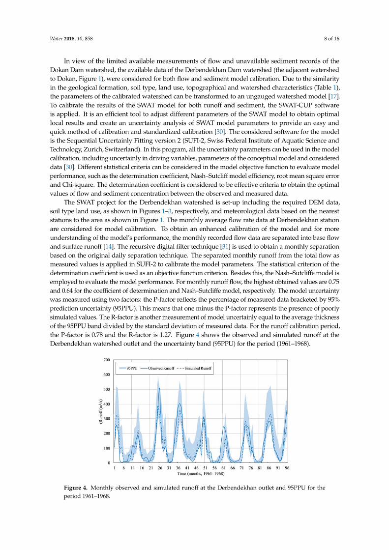
The SWAT project for the Derbendekhan watershed is set-up including the required DEM data,soil type land use, as shown in Figures 1–3, respectively, and meteorological data based on the neareststations to the area as shown in Figure 1. The monthly average flow rate data at Derbendekhan stationare considered for model calibration. To obtain an enhanced calibration of the model and for moreunderstanding of the model’s performance, the monthly recorded flow data are separated into base flowand surface runoff [14]. The recursive digital filter technique [31] is used to obtain a monthly separationbased on the original daily separation technique. The separated monthly runoff from the total flow asmeasured values is applied in SUFI-2 to calibrate the model parameters. The statistical criterion of thedetermination coefficient is used as an objective function criterion. Besides this, the Nash–Sutcliffe model isemployed to evaluate the model performance. For monthly runoff flow, the highest obtained values are 0.75and 0.64 for the coefficient of determination and Nash–Sutcliffe model, respectively. The model uncertaintywas measured using two factors: the P-factor reflects the percentage of measured data bracketed by 95%prediction uncertainty (95PPU). This means that one minus the P-factor represents the presence of poorlysimulated values. The R-factor is another measurement of model uncertainly equal to the average thicknessof the 95PPU band divided by the standard deviation of measured data. For the runoff calibration period,the P-factor is 0.78 and the R-factor is 1.27. Figure 4 shows the observed and simulated runoff at theDerbendekhan watershed outlet and the uncertainty band (95PPU) for the period (1961–1968).

Water 2018, 10, x FOR PEER REVIEW    8 of 16 

ungauged watershed model  [17]. To calibrate  the results of  the SWAT model  for both runoff and 

sediment, the SWAT‐CUP software is applied. It is an efficient tool to adjust different parameters of 

the SWAT model to obtain optimal local results and create an uncertainty analysis of SWAT model 

parameters to provide an easy and quick method of calibration and standardized calibration [30]. The 

considered  software  for  the model  is  the Sequential Uncertainly Fitting version  2  (SUFI‐2, Swiss 

Federal Institute of Aquatic Science and Technology, Zurich, Switzerland). In this program, all the 

uncertainty  parameters  can  be  used  in  the model  calibration,  including  uncertainly  in  driving 

variables, parameters of the conceptual model and considered data [30]. Different statistical criteria 

can  be  considered  in  the model  objective  function  to  evaluate model  performance,  such  as  the 

determination coefficient, Nash–Sutcliff model efficiency, root mean square error and Chi‐square. 

The determination coefficient is considered to be effective criteria to obtain the optimal values of flow 

and sediment concentration between the observed and measured data. 

The SWAT project for the Derbendekhan watershed is set‐up including the required DEM data, 

soil type land use, as shown in Figures 1–3, respectively, and meteorological data based on the nearest 

stations to the area as shown in Figure 1. The monthly average flow rate data at Derbendekhan station 

are considered for model calibration. To obtain an enhanced calibration of the model and for more 

understanding of the model’s performance, the monthly recorded flow data are separated into base 

flow and surface runoff [14]. The recursive digital filter technique [31] is used to obtain a monthly 

separation based on the original daily separation technique. The separated monthly runoff from the 

total flow as measured values is applied in SUFI‐2 to calibrate the model parameters. The statistical 

criterion of the determination coefficient is used as an objective function criterion. Besides this, the 

Nash–Sutcliffe model is employed to evaluate the model performance. For monthly runoff flow, the 

highest obtained values are 0.75 and 0.64  for  the  coefficient of determination and Nash–Sutcliffe 

model, respectively. The model uncertainty was measured using two factors: the P‐factor reflects the 

percentage of measured data bracketed by 95% prediction uncertainty (95PPU). This means that one 

minus  the  P‐factor  represents  the  presence  of  poorly  simulated  values.  The  R‐factor  is  another 

measurement of model uncertainly equal to the average thickness of the 95PPU band divided by the 

standard deviation of measured data. For the runoff calibration period, the P‐factor is 0.78 and the R‐

factor  is 1.27. Figure 4 shows  the observed and simulated runoff at  the Derbendekhan watershed 

outlet and the uncertainty band (95PPU) for the period (1961–1968). 

 

Figure 4. Monthly observed and  simulated  runoff at  the Derbendekhan outlet and 95PPU  for  the 

period 1961–1968. 

Figure 4. Monthly observed and simulated runoff at the Derbendekhan outlet and 95PPU for theperiod 1961–1968.

Water 2018, 10, 858 9 of 16

The available measured sediment concentration data of the Diyala River at Derbendekhan station,as presented by Assad [32], were utilized to calibrate the SWAT model parameters for the same periodof runoff flow calibration. Figure 5 shows the measured and optimal simulated values of sedimentload concentration at Derbendekhan outlet. The same statistical criteria are implemented, and theoptimal resultant values are 0.65 and 0.63 for determination coefficient and Nash–Sutcliffe modelefficiency, respectively, while the P-factor and R-factor equal to 0.68 and 2.27 respectively.

Water 2018, 10, x FOR PEER REVIEW    9 of 16 

The  available measured  sediment  concentration  data  of  the Diyala  River  at Derbendekhan 

station, as presented by Assad [32], were utilized to calibrate the SWAT model parameters for the 

same period of runoff flow calibration. Figure 5 shows the measured and optimal simulated values 

of sediment load concentration at Derbendekhan outlet. The same statistical criteria are implemented, 

and the optimal resultant values are 0.65 and 0.63 for determination coefficient and Nash–Sutcliffe 

model efficiency, respectively, while the P‐factor and R‐factor equal to 0.68 and 2.27 respectively. 

 

Figure  5.  Observed  and  simulated  sediment  concentration  for  period  (1961–1968)  at  the 

Derbendekhan watershed. 

The most effective parameters are  selected  for  the  runoff and  sediment model  calibration as 

proposed by [28] in addition to other parameters. The resultant best‐fitted values (optimal values) of 

the parameters and the considered range are shown in Table 3. Parameters listed in Table 3 are also 

mentioned in other previous literature [14,33]. 

Table 3. The range, optimal (fitted) values and sensitivity analysis of considered parameters. 

Parameter  Description Min_

Value 

Max_

Value 

Fitted_

Value 

V_GWQMN.gw  Threshold depth in shallow aquifer (mm).  0  2  1.698 

V_CH_COV1.rte  Channel erodibility factor.  0.05  0.6  0.38715 

R_USLE_K(..).sol  USLE, equation soil erodibility (k) factor.  −0.8  0.8  −0.1168 

R_LAT_SED.hru  Sediment conc. In lateral and ground flow.  0  5000  2525 

R_SPCON.bsn Linear par. for calculating max. amount of sediment that 

can be re‐entrained during channel sediment routing.   

0.000

1 0.01 

0.00874

3 

V_SPEXP.bsn 

Exponential Par. for calculating max. amount of 

sediment that can be re‐entrained during channel 

sediment routing.   

1  2  1.549 

V_GW_REVAP.gw  Groundwater “revap” coefficient.  0.02  0.2  0.07166 

V_ALPHA_BF.gw  Base flow alpha factor (days).  0  1  0.555 

V__CH_COV2.rte  Channel cover factor.  0.001  1 0.28171

9 

V_GW_DELAY.gw  Groundwater delay (days).  0.02  0.2  0.07166 

R_SOL_BD(..).sol  Moist bulk density.  −0.5  1  −0.3755 

R_USLE_C(..)plant.dat  Min value of USLE‐C factor for land cover/plant.  −0.5  0.5 0.15100

0 

R_CH_N2.rte  Manning’s “n” value for the main channel.  −0.5  0.5  −0.279 

R_USLE_P.mgt  USLE, support practice parameter.  0  1  0.941 

R_SOL_K(..).sol  Saturated hydraulic conductivity.  −0.5  0.5  0.177 

R_CN2.mgt  SCS runoff curve number.  −0.2  0.2  0.198 

R_SOL_AWC(..).sol  Available water content of the soil layer.  −0.5  1  0.5005 

Note: R: Relative, V: Replace. (…) for different soil or plant type. 

Figure 5. Observed and simulated sediment concentration for period (1961–1968) at the Derbendekhan watershed.

The most effective parameters are selected for the runoff and sediment model calibration asproposed by [28] in addition to other parameters. The resultant best-fitted values (optimal values) ofthe parameters and the considered range are shown in Table 3. Parameters listed in Table 3 are alsomentioned in other previous literature [14,33].

Table 3. The range, optimal (fitted) values and sensitivity analysis of considered parameters.

Parameter Description Min_Value Max_Value Fitted_Value

V_GWQMN.gw Threshold depth in shallow aquifer (mm). 0 2 1.698V_CH_COV1.rte Channel erodibility factor. 0.05 0.6 0.38715R_USLE_K(..).sol USLE, equation soil erodibility (k) factor. −0.8 0.8 −0.1168R_LAT_SED.hru Sediment conc. In lateral and ground flow. 0 5000 2525

R_SPCON.bsnLinear par. for calculating max. amount ofsediment that can be re-entrained duringchannel sediment routing.

0.0001 0.01 0.008743

V_SPEXP.bsnExponential Par. for calculating max. amountof sediment that can be re-entrained duringchannel sediment routing.

1 2 1.549

V_GW_REVAP.gw Groundwater “revap” coefficient. 0.02 0.2 0.07166V_ALPHA_BF.gw Base flow alpha factor (days). 0 1 0.555V__CH_COV2.rte Channel cover factor. 0.001 1 0.281719V_GW_DELAY.gw Groundwater delay (days). 0.02 0.2 0.07166R_SOL_BD(..).sol Moist bulk density. −0.5 1 −0.3755

R_USLE_C(..)plant.dat Min value of USLE-C factor for landcover/plant. −0.5 0.5 0.151000

R_CH_N2.rte Manning’s “n” value for the main channel. −0.5 0.5 −0.279R_USLE_P.mgt USLE, support practice parameter. 0 1 0.941R_SOL_K(..).sol Saturated hydraulic conductivity. −0.5 0.5 0.177R_CN2.mgt SCS runoff curve number. −0.2 0.2 0.198R_SOL_AWC(..).sol Available water content of the soil layer. −0.5 1 0.5005

Note: R: Relative, V: Replace. (..) for different soil or plant type.

Water 2018, 10, 858 10 of 16

4.2. Runoff Validation

A SWAT model project is set-up for the Dokan Dam watershed, the main part of the study area.The limited recorded data of the monthly flow rate at the outlet of the Dokan watershed and theabsence of any sediment load measurements leads to utilizing the regionalization technique to transferthe effective parameters from the adjacent gauged (Derbendekhan) watershed. Due to its similarityin geological formation, soil type, land use, watershed characteristics and weather data, the effectivehydrological parameters obtained from the Derbendekhan (gauged) watershed can be transformed tothe Dokan (ungauged) watershed. The process of parameter transformation is called regionalization.There are a number of presented methods for the regionalization of the watershed hydrologicalparameters: Kokkonen [34] applies the regression approach, while Parajka et al. [35] employs kringingand a similarity approach and Heuvelmans et al. [36] investigates the application of artificial neuralnets and other methods. Since the Derbendekhan watershed is adjacent to the Dokan watershed(Figure 1), and the physical, topographical properties and rainfall are similar (Table 1) along withthe geological formation, land use/land cover, and soil type, both watersheds have similar flow andsediment parameters. In this case, the effective parameters can be transformed from a donor watershedto an ungauged watershed. The fitted values of the Derbendekhan parameters calibrated by the SUFI-2program are transferred to the Dokan watershed SWAT project. The SUFI-2 program is implementedfor the calibration, uncertainly analysis and regionalization of the considered parameters of the SWATmodel for the Debendekhan watershed for runoff and sediment load of concentration. Here, the SUFI-2algorithm is used for the calibration, validation and measurement of the uncertainty for input data,model and sensitive parameters. The degree of uncertainty is measured by two values: P-factor andR-factor. The percent of measured values bracketed by 95% prediction uncertainly represent (95PPU),which is the P-factor while the ratio of 95PPU thickness divided by standard deviation of measuredvalues is equal to the R-factor. When the simulated values are exactly the measured ones, the value ofP-factor equals 1 and the value of R-factor equals zero [37].

Based on the transformed parameters, the simulated runoff flows are compared with measuredvalues at the Dokan watershed outlet after the separation of the base flow for the period 1961–1964(Figure 6) to evaluate the effectiveness of the transformation of the hydrological parameters. For thevalidation period of runoff, the obtained values of the determination coefficient and Nash–Sutcliffemodel efficiency are 0.68 and 0.64, respectively, indicating that the transformation process is successful.The P-factor and R-factor for the model uncertainty also indicate a reasonable model performance:the P-factor is 0.71 and R-factor is 0.97.

Water 2018, 10, x FOR PEER REVIEW    10 of 16 

4.2. Runoff Validation 

A SWAT model project is set‐up for the Dokan Dam watershed, the main part of the study area. 

The  limited recorded data of  the monthly  flow rate at  the outlet of  the Dokan watershed and  the 

absence  of  any  sediment  load measurements  leads  to  utilizing  the  regionalization  technique  to 

transfer  the effective parameters  from  the adjacent gauged  (Derbendekhan) watershed. Due  to  its 

similarity in geological formation, soil type, land use, watershed characteristics and weather data, the 

effective  hydrological  parameters  obtained  from  the Derbendekhan  (gauged) watershed  can  be 

transformed to the Dokan (ungauged) watershed. The process of parameter transformation is called 

regionalization  [14].  There  are  a  number  of  presented  methods  for  the  regionalization  of  the 

watershed hydrological parameters: Kokkonen [34] applies the regression approach, while Parajka 

et al. [35] employs kringing and a similarity approach and Heuvelmans et al. [36] investigates the 

application of artificial neural nets and other methods. Since the Derbendekhan watershed is adjacent 

to the Dokan watershed (Figure 1), and the physical, topographical properties and rainfall are similar 

(Table 1) along with the geological formation, land use/land cover, and soil type, both watersheds 

have similar flow and sediment parameters. In this case, the effective parameters can be transformed 

from  a  donor  watershed  to  an  ungauged  watershed.  The  fitted  values  of  the  Derbendekhan 

parameters calibrated by the SUFI‐2 program are transferred to the Dokan watershed SWAT project. 

The SUFI‐2 program is implemented for the calibration, uncertainly analysis and regionalization of 

the  considered  parameters  of  the  SWAT model  for  the Debendekhan watershed  for  runoff  and 

sediment load of concentration. Here, the SUFI‐2 algorithm is used for the calibration, validation and 

measurement  of  the  uncertainty  for  input  data, model  and  sensitive  parameters.  The  degree  of 

uncertainty  is measured  by  two  values:  P‐factor  and  R‐factor.  The  percent  of measured  values 

bracketed by 95% prediction uncertainly represent (95PPU), which is the P‐factor while the ratio of 

95PPU thickness divided by standard deviation of measured values is equal to the R‐factor. When 

the simulated values are exactly the measured ones, the value of P‐factor equals 1 and the value of R‐

factor equals zero [37]. 

Based on the transformed parameters, the simulated runoff flows are compared with measured 

values at the Dokan watershed outlet after the separation of the base flow for the period 1961–1964 

(Figure 6) to evaluate the effectiveness of the transformation of the hydrological parameters. For the 

validation period of runoff, the obtained values of the determination coefficient and Nash–Sutcliffe 

model  efficiency  are  0.68  and  0.64,  respectively,  indicating  that  the  transformation  process  is 

successful. The P‐factor and R‐factor  for  the model uncertainty also  indicate a  reasonable model 

performance: the P‐factor is 0.71 and R‐factor is 0.97. 

 

Figure 6. Monthly observed and simulated runoff at the Dokan outlet and 95PPU for the period 1962–

1965. Figure 6. Monthly observed and simulated runoff at the Dokan outlet and 95PPU for theperiod 1962–1965.

Water 2018, 10, 858 11 of 16

5. Results and Discussion

After Durbendekhan SWAT project calibration for runoff and sediment data, the best-fitted valuesof the hydrological watershed parameters are transformed by the regionalization technique to theDokan SWAT project, the main project of the study. The sensitivity analysis is also studied for themost effective parameters on both the runoff and sediment load. The sensitivities are accomplished toidentify the effective parameters on runoff and sediment load values for the watershed. The parametersensitivity is estimated in the SUFI-2 model based on the multiple regression system presented byAbbaspour [38] to evaluate the effect of the considered parameter value (bi) on the objective function(g); its sensitivity is in the following form:

g = α +m

∑i=1

βibi (6)

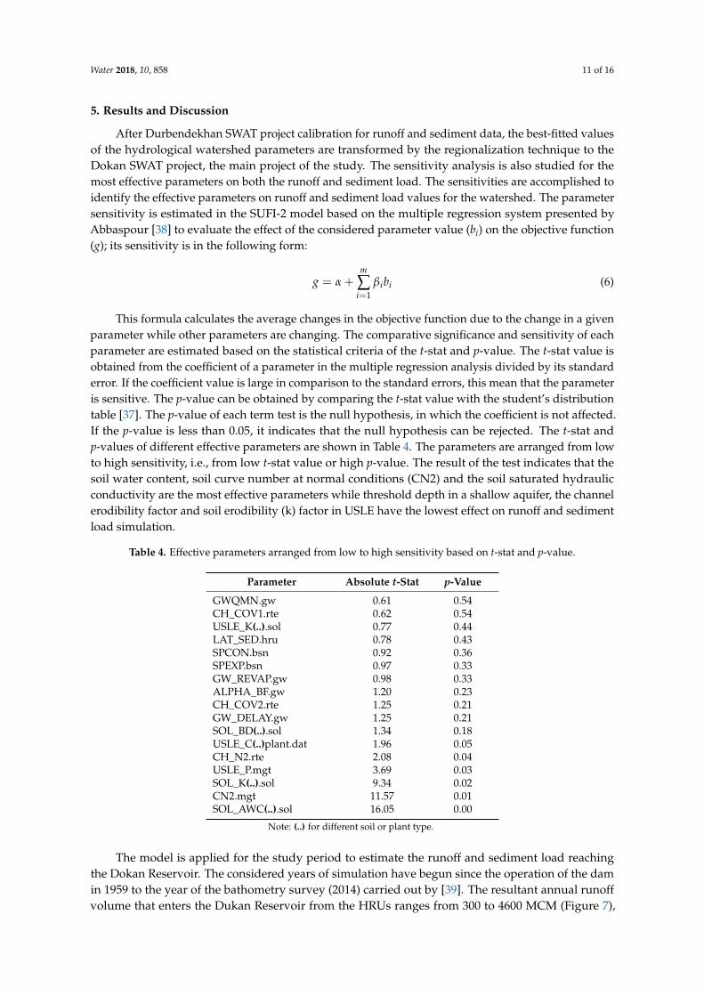
This formula calculates the average changes in the objective function due to the change in a givenparameter while other parameters are changing. The comparative significance and sensitivity of eachparameter are estimated based on the statistical criteria of the t-stat and p-value. The t-stat value isobtained from the coefficient of a parameter in the multiple regression analysis divided by its standarderror. If the coefficient value is large in comparison to the standard errors, this mean that the parameteris sensitive. The p-value can be obtained by comparing the t-stat value with the student’s distributiontable [37]. The p-value of each term test is the null hypothesis, in which the coefficient is not affected.If the p-value is less than 0.05, it indicates that the null hypothesis can be rejected. The t-stat andp-values of different effective parameters are shown in Table 4. The parameters are arranged from lowto high sensitivity, i.e., from low t-stat value or high p-value. The result of the test indicates that thesoil water content, soil curve number at normal conditions (CN2) and the soil saturated hydraulicconductivity are the most effective parameters while threshold depth in a shallow aquifer, the channelerodibility factor and soil erodibility (k) factor in USLE have the lowest effect on runoff and sedimentload simulation.

Table 4. Effective parameters arranged from low to high sensitivity based on t-stat and p-value.

Parameter Absolute t-Stat p-Value

GWQMN.gw 0.61 0.54CH_COV1.rte 0.62 0.54USLE_K(..).sol 0.77 0.44LAT_SED.hru 0.78 0.43SPCON.bsn 0.92 0.36SPEXP.bsn 0.97 0.33GW_REVAP.gw 0.98 0.33ALPHA_BF.gw 1.20 0.23CH_COV2.rte 1.25 0.21GW_DELAY.gw 1.25 0.21SOL_BD(..).sol 1.34 0.18USLE_C(..)plant.dat 1.96 0.05CH_N2.rte 2.08 0.04USLE_P.mgt 3.69 0.03SOL_K(..).sol 9.34 0.02CN2.mgt 11.57 0.01SOL_AWC(..).sol 16.05 0.00

Note: (..) for different soil or plant type.

The model is applied for the study period to estimate the runoff and sediment load reachingthe Dokan Reservoir. The considered years of simulation have begun since the operation of the damin 1959 to the year of the bathometry survey (2014) carried out by [39]. The resultant annual runoffvolume that enters the Dukan Reservoir from the HRUs ranges from 300 to 4600 MCM (Figure 7),

Water 2018, 10, 858 12 of 16

depending on rainfall intensity, depth and distribution through the rainy season. The runoff averagevolume from the watershed represents 35% of the live storage capacity of the dam, indicating thatwatershed runoff makes a significant contribution to reservoir inflow.

The SWAT model is an efficient tool to estimate the runoff hydrograph, but, in some hydrologicalstudies, such as scheduling reservoir operations to supply the demand rate, the assessment of waterresource income only is required. A regression formula is determined based upon the input–outputdata of SWAT model of the study area. This is a simple and quick tool to correlate the annual runoffdepth with annual rainfall with good correlation (R2 = 0.9) results without the need for more detailedinput data as required in SWAT projects. The relationship used is in the following form:

RunAnn = 0.075 × R1.21Ann − 1.92 R2 = 0.90 ( f or RAnn > 16 mm) (7)

where

RunAnn: Annual runoff depth mm);RAnn: Annual rainfall depth (mm).

Water 2018, 10, x FOR PEER REVIEW    12 of 16 

volume from the watershed represents 35% of the live storage capacity of the dam, indicating that 

watershed runoff makes a significant contribution to reservoir inflow.   

The  SWAT  model  is  an  efficient  tool  to  estimate  the  runoff  hydrograph,  but,  in  some 

hydrological  studies,  such  as  scheduling  reservoir  operations  to  supply  the  demand  rate,  the 

assessment of water  resource  income only  is  required. A  regression  formula  is determined based 

upon  the  input–output data of SWAT model of  the study area. This  is a simple and quick  tool  to 

correlate the annual runoff depth with annual rainfall with good correlation (R2 = 0.9) results without 

the need for more detailed input data as required in SWAT projects. The relationship used is in the 

following form: 

0.075 . 1.92R 0.90 16   (7) 

where 

: Annual runoff depth mm); 

  : Annual rainfall depth (mm). 

 

Figure 7. Annual runoff volume and sediment load delivered to the Dokan Reservoir for the period 

1959–2014. 

The formula is suitable when the annual runoff depth is greater than 15 mm to avoid negative 

runoff; this value is already much lower than the minimum historical recorded value. 

The  sediment  load  delivered  to  the  Dokan  reservoir  is  also  estimated  based  on  MUSLE 

programmed into the SWAT model for each single storm. The results are presented here annually. 

The average annual sediment load concentration is 650 mg/ℓ. This concentration can be considered 

relatively  low  in comparison with other  locations or measurements  in  the  region as proposed by 

[40,41] as well as the worldwide rate [42]. This is due to the nature of the rocks of the area and the 

effect of plant cover, such as winter pasture and plants and some forest trees throughout the region 

which reduce the detachment of soil particles transported with runoff flow. The estimated annual 

sediment load delivered to the Dokan reservoir from the watershed ranges from 3.6 to 0.16 × 106 ton 

for studied period, Figure 7. The average annual value is 1.63 × 106 ton.   

The sediment  trap efficiency of  the reservoir  is estimated based on  the method presented by 

Garg V. and Jothiprakash V. [43]. This depends on reservoir storage capacity and annual inflow. The 

trap efficiency of the Dokan reservoir changes through the study period from 1 to 0.985. 

Based on the results obtained from the simulation model, the estimated sediment load volume 

deposited in the reservoir for the considered period is about 10% of the dead storage capacity. This 

value  is  for  the watershed only, which  is  considered  a  reasonable value  and does not  affect  the 

Figure 7. Annual runoff volume and sediment load delivered to the Dokan Reservoir for theperiod 1959–2014.

The formula is suitable when the annual runoff depth is greater than 15 mm to avoid negativerunoff; this value is already much lower than the minimum historical recorded value.

The sediment load delivered to the Dokan reservoir is also estimated based on MUSLEprogrammed into the SWAT model for each single storm. The results are presented here annually.The average annual sediment load concentration is 650 mg/`. This concentration can be consideredrelatively low in comparison with other locations or measurements in the region as proposed by [40,41]as well as the worldwide rate [42]. This is due to the nature of the rocks of the area and the effectof plant cover, such as winter pasture and plants and some forest trees throughout the region whichreduce the detachment of soil particles transported with runoff flow. The estimated annual sedimentload delivered to the Dokan reservoir from the watershed ranges from 3.6 to 0.16 × 106 ton for studiedperiod, Figure 7. The average annual value is 1.63 × 106 ton.

The sediment trap efficiency of the reservoir is estimated based on the method presented by GargV. and Jothiprakash V. [43]. This depends on reservoir storage capacity and annual inflow. The trapefficiency of the Dokan reservoir changes through the study period from 1 to 0.985.

Based on the results obtained from the simulation model, the estimated sediment load volumedeposited in the reservoir for the considered period is about 10% of the dead storage capacity.This value is for the watershed only, which is considered a reasonable value and does not affect

Water 2018, 10, 858 13 of 16

the designed project life. However, the Lesser Zab load should be also considered to evaluate the totalamount of sediment load delivered and deposited within the reservoir. The total amount of sedimentdeposited in the Dokan reservoir for the period (1959–2014) is 209 MCM [38]. This means that thesediment load delivered into the reservoir from the watershed based on simulated results is about34% of the total sediments deposited within the reservoir, which mean that the watershed sedimentcontribution is an effective value.

Due to the huge amount of data required, including topographical, metrological and hydrologicaldata, different maps of soil, and land use to estimate the sediment load based on the applied model,a simple regression formula is used. It is based on simulated values to correlate the sediment load perunit area of the Dokan watershed with annual runoff depth in the following form:

SedAnn = 0.056·R1.195Ann − 7.33 R2 = 0.97 ( f or RAnn > 60mm) (8)

where

SedAnn: Annual sediment load per unit area, (ton/km2);RAnn: Annual rainfall depth (mm).

The formula is suitable when the annual runoff depth is greater than 60 mm; this value is alreadylower than the minimum historical recorded value in Dokan area.

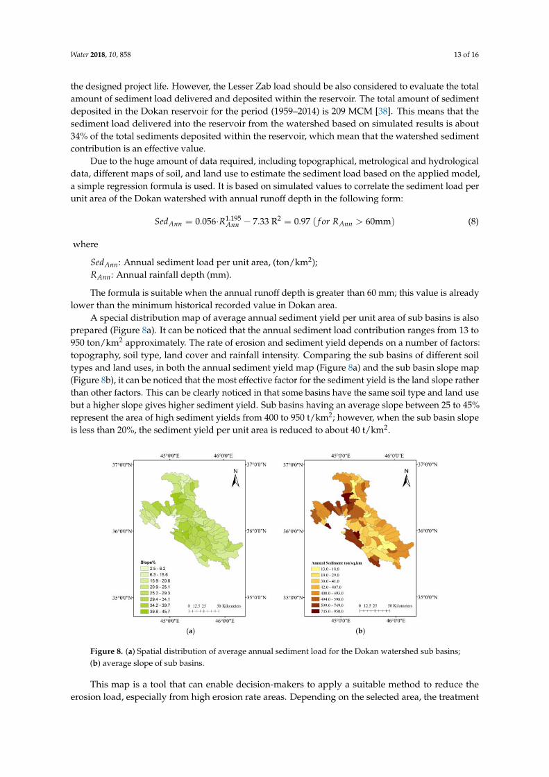
A special distribution map of average annual sediment yield per unit area of sub basins is alsoprepared (Figure 8a). It can be noticed that the annual sediment load contribution ranges from 13 to950 ton/km2 approximately. The rate of erosion and sediment yield depends on a number of factors:topography, soil type, land cover and rainfall intensity. Comparing the sub basins of different soiltypes and land uses, in both the annual sediment yield map (Figure 8a) and the sub basin slope map(Figure 8b), it can be noticed that the most effective factor for the sediment yield is the land slope ratherthan other factors. This can be clearly noticed in that some basins have the same soil type and land usebut a higher slope gives higher sediment yield. Sub basins having an average slope between 25 to 45%represent the area of high sediment yields from 400 to 950 t/km2; however, when the sub basin slopeis less than 20%, the sediment yield per unit area is reduced to about 40 t/km2.

Water 2018, 10, x FOR PEER REVIEW    13 of 16 

designed project life. However, the Lesser Zab load should be also considered to evaluate the total 

amount of sediment load delivered and deposited within the reservoir. The total amount of sediment 

deposited in the Dokan reservoir for the period (1959–2014) is 209 MCM [38]. This means that the 

sediment load delivered into the reservoir from the watershed based on simulated results is about 

34% of the total sediments deposited within the reservoir, which mean that the watershed sediment 

contribution is an effective value. 

Due  to  the  huge  amount  of  data  required,  including  topographical,  metrological  and 

hydrological data, different maps of soil, and land use to estimate the sediment load based on the 

applied model, a simple regression formula is used. It is based on simulated values to correlate the 

sediment load per unit area of the Dokan watershed with annual runoff depth in the following form: 

0.056. . 7.33R 0.97 60   (8) 

where 

: Annual sediment load per unit area, (ton/km2); 

  : Annual rainfall depth (mm). 

The formula is suitable when the annual runoff depth is greater than 60 mm; this value is already 

lower than the minimum historical recorded value in Dokan area. 

A special distribution map of average annual sediment yield per unit area of sub basins is also 

prepared (Figure 8a). It can be noticed that the annual sediment load contribution ranges from 13 to 

950 ton/km2 approximately. The rate of erosion and sediment yield depends on a number of factors: 

topography, soil type, land cover and rainfall intensity. Comparing the sub basins of different soil 

types and land uses, in both the annual sediment yield map (Figure 8a) and the sub basin slope map 

(Figure 8b), it can be noticed that the most effective factor for the sediment yield is the land slope 

rather than other factors. This can be clearly noticed in that some basins have the same soil type and 

land use but a higher slope gives higher sediment yield. Sub basins having an average slope between 

25 to 45% represent the area of high sediment yields from 400 to 950 t/km2; however, when the sub 

basin slope is less than 20%, the sediment yield per unit area is reduced to about 40 t/km2.   

This map  is a  tool  that can enable decision‐makers  to apply a suitable method  to reduce  the 

erosion load, especially from high erosion rate areas. Depending on the selected area, the treatment 

may include practicing strip planting, terracing, or contour forming to reduce the effect of slope on 

surface runoff flow velocity, erosion and sediment transport capacity.   

   (a)  (b) 

Figure 8. (a) Spatial distribution of average annual sediment load for the Dokan watershed sub basins; 

(b) average slope of sub basins. Figure 8. (a) Spatial distribution of average annual sediment load for the Dokan watershed sub basins;(b) average slope of sub basins.

This map is a tool that can enable decision-makers to apply a suitable method to reduce theerosion load, especially from high erosion rate areas. Depending on the selected area, the treatment

Water 2018, 10, 858 14 of 16

may include practicing strip planting, terracing, or contour forming to reduce the effect of slope onsurface runoff flow velocity, erosion and sediment transport capacity.

6. Conclusions

The soil and water assessment tool (SWAT) model is applied to assess the runoff and sedimentdelivered from the Dokan Dam watershed. Due to the limited recorded flow data and the absence ofsediment measurements data at a station near the inlet of Dokan Reservoir, the model is calibratedfor both runoff and sediment load for the Derbendekhan watershed adjacent to the Dokan watershed.The regionalization technique is employed to transfer the calibrated parameters of the SWAT projectfrom a gauged (Derbendekhan) to an ungauged (Dokan) watershed. The resultant monthly runoffflow for the Dokan SWAT project is based on transformed parameters which were compared withmeasured values to evaluate the regionalization technique and model performance. The determinationcoefficient (R2) and Nash–Sutcliffe model efficiency (Eff.) are 0.68 and 0.64, respectively, indicating areasonable model performance with this technique. The average watershed contribution for annualrunoff represents 35% of the dam life storage; this percentage is considered effective in the damoperation schedule. The total sediment load delivered to the Dokan reservoir from the watershed forthe studied period is about 72 MCM. This load forms about 10% of the dead storage capacity of thereservoir. Generally, the total sediment load delivered and deposited in the reservoir for the periodof dam operation is considered acceptable within the allowed limits. The map of special distributionof annual sediment load yield per unit area of each sub basins is presented; the average slopes mapreflects a good agreement with the map of annual sediment load yield in comparison to other effectivefactors to be considered. This indicates that the land slope is the most effective factor on erosion andsediment transport. This can be used for soil conservation treatment to reduce the erosion rate.

Author Contributions: M.E.-A. and R.H. did the field, methodology and modelling, A.A. helped in the modelling,N.A.-A. and S.K. did the supervision.

Funding: This research received no external funding.

Acknowledgments: The authors would like to express their thanks to John McManus (University of St. Andrews,St. Andrews, UK) and Ian Foster (Northampton University, Northampton, UK) for reading the manuscript andfor their fruitful discussions and suggestions, and to Lulea University of Technology for some of the financialsupport for this research.

Conflicts of Interest: The authors declare no conflict of interest.

References

1. Schleiss, A.J.; Franca, M.J.; Juez, C.; De Cesare, G. Reservoir Sedimentation—Vision Paper. J. Hydraul. Res.2016, 54, 595–614. [CrossRef]

2. Beasley, D.B.; Huggins, L.F.; Monke, E.J. ANSWERS: A model for watershed planning. Trans. ASAE 1980,23, 938–944. [CrossRef]

3. Morgan, R.P.C.; Quinton, J.N.; Smith, R.E.; Govers, G.; Poesen, J.W.; Auerswald, K.; Chisci, G.; Torri, D.;Styczen, M.E.; Folly, A.J. The European soil erosion model (EUROSEM): A dynamic approach for predictingsediment transport from fields and small catchments. Earth Surface Process. Landf. 1998, 23, 527–544.[CrossRef]

4. Knisel, W.G. CREAMS: A Field-Scale Model for Chemical, Runoff and Erosion from Agricultural Management Systems;USDA Conservation Research Report; Conservation Model Development: Washington, WA, USA, 1980.

5. Wicks, J.M.; Bathurst, J.C. SHESED: A physically based, distributed erosion and sediment yield componentfor the SHE hydrological modelling system. J. Hydrol. 1996, 175, 213–238. [CrossRef]

6. Arnold, J.G.; Srinisvan, R.; Muttiah, R.S. Large area hydrologic modeling and assessment. Part I: Modeldevelopment. Am. Water Resour. Assoc. 1998, 34, 73–89. [CrossRef]

7. Easton, Z.M.; Fukal, D.R.; White, E.D.; Collick, A.S.; Ashagre, B.B.; McCartney, M.; Awulachew, S.B.;Ahmed, A.A.; Steenhuis, T.S. A multi basin SWAT model analysis of runoff and sedimentation in the BlueNile, Ethiopia. Hydrol. Earth Syst. Sci. 2010, 14, 827–1841. [CrossRef]

Water 2018, 10, 858 15 of 16

8. Swami, V.A.; Kulkarni, S.S. Simulation of runoff and sediment yield for a Kaneri Watershed Using SWATModel. J. Geosci. Environ. Protect. 2016, 4, 1–15. [CrossRef]

9. Durao, A.; Leitao, P.C.; Brito, D.; Fernandes, R.; Neves, R.; Morais, M.M. Estimation of Transported PollutantLoad in Ardila Catchment Using the SWAT Model. In Proceedings of the International SWAT Conference,Toledo, Spain, 15–17 June 2011.

10. Wang, X.; Amonett, C.; Williams, J.R.; Fox, W.E.; Tu, C. Assessing Impacts of Rangeland ConservationPractices Prior to Implementation: A Simulation Case Study using APEX. In Proceedings of the InternationalSWAT Conference, Toledo, Spain, 15–17 June 2011.

11. Samaras, A.G.; Koutitas, C.G. The impact of watershed management on coastal morphology: A case studyusing an integrated approach and numerical modeling. Geomorphology 2014, 211, 52–63. [CrossRef]

12. Samaras, A.G.; Koutitas, C.G. Modeling the impact of climate change on sediment transport and morphologyin coupled watershed-coast systems: A case study using an integrated approach. Int. J. Sediment Res. 2014,29, 304–315. [CrossRef]

13. Arnold, J.G.; Youssef, M.A.; Yen, H.; White, A.Y.; Sheshukov, A.M.; Sadeghi, D.N.; Moriasi, D.N.; Steiner, J.L.;Amatya, D.M.; Haney, E.B.; et al. Hydrological processes and model representation: Impact of soft data oncalibration. Trans. ASABE 2015, 58, 1637–1660.

14. Emam, A.R.; Kappas, M.; Linh, N.H.K.; Renchin, T. Hydrological Modeling and Runoff Mitigation in anUngauged Basin of Central Vietnam Using SWAT Model. Hydrology 2017, 4, 1–17.

15. Emam, A.R.; Kappas, M.; Linh, N.H.K.; Renchin, T. Hydrological Modeling in an Ungauged Basin of CentralVietnam. Hydrol. Earth Syst. Sci. Discuss. 2016, 1–33. [CrossRef]

16. Prabhanjan, A.; Rao, E.P.; Eldho, T.I. Application of SWAT Model and Geospatial Techniques forSediment-Yield Modeling in Ungauged Watersheds. J. Hydrol. Eng. 2014, 20, C6014005. [CrossRef]

17. B’ardossy, A. Calibration of hydrological model parameters for ungauged catchments. Hydrol. Earth Syst. Sci.2007, 11, 703–710. [CrossRef]

18. Juez, C.; Tena, A.; Fernández-Pato, J.; Batalla, R.J.; Garcia-Navarro, P. Application of A Distributed2d Overland Flow Model for Rainfall/Runoff and Erosion Simulation in A Mediterranean Watershed.Cuadernos de Investigación Geográfica 2018. (In Spanish) [CrossRef]

19. Al-Ansari, N. Hydropolitics of the Tigris and Euphrates Basins. Engineering 2016, 8, 140–172. [CrossRef]20. Bazzaz, F. Global climatic changes and its consequences for water availability in the Arab world. In

Water in the Arab Word: Perspectives and Prognoses; Roger, R., Lydon, P., Eds.; Harvard University:Cambridge, MA, USA, 1993; pp. 243–252.

21. Al-Ansari, N.; Knutsson, S. Toward Prudent management of Water Resources in Iraq. Adv. Sci. Eng. Res.2011, 1, 53–67.

22. World Bank. Iraq. Country Water Resources, Assistance Strategy: Addressing Major Threats to People’s Livelihoods;Water, Environment, Social and Rural Development Department: Washington, DC, USA, 2006.

23. UNESCO. Iraq’s Water in the International Press; UNESCO Office for Iraq: Erbil, Iraq, 2010.24. Hassan, R.; Al-Ansari, N.; Ali, S.A.; Ali, A.A.; Abdullah, T.; Knutsson, S. Dukan Dam Reservoir Bed Sediment,

Kurdistan Region, Iraq. Engineering 2016, 8, 582–596. [CrossRef]25. Karim, K.H.; Al-Hakari, S.H.S.; Kharajiany, S.O.A.; Khanaqa, A.P. Surface Analysis and Critical Review of

the Darbandikhan (Khanaqin) Fault, Kurdistan Region, Northeast Iraq. Kurdistan Acad. 2016, 12, 61–75.26. Berding, F. Reconnaissance Soil Map of the Three Northern Governorates; FAO Erbil Coordination Office: Erbil,

Iraq, 2001.27. Food and Agriculture Organization of the United Nations. The Digital Soil Map of the World and Derived Soil

Properties; Version 3.6; FAO: Rome, Italy, 2003.28. Ministry of Agricultural and Irrigation, Republic of Iraq. Map of Soil and Land Use; Ministry of Agricultural

and Irrigation: Baghdad, Iraq, 1990.29. Neitsch, S.L.; Arnold, J.G.; Kiniry, J.R.; Williams, J.R. Soil and Water Assessment Tool; Theoretical

Documentation Version 2009; Texas Water Resources Institute: College Station, TX, USA, 2011.30. Abbaspour, K.C.; Vejdani, M.; Haghighat, S. SWAT-CUP Calibration and Uncertainty Programs for SWAT.

In Proceedings of the International Congress on Modelling and Simulation (MODSIM 2007), Melbourne,Australia, 10 December 2007.

31. Smakhtin, V.U. Estimating continuous monthly baseflow time series and their possible applications in thecontext of the ecological reserve. Water SA 2001, 27, 213–218. [CrossRef]

Water 2018, 10, 858 16 of 16

32. Assad, M.N. Sediments and Sediment Discharge in the River Diyala. Master’s Thesis, Baghdad University,Baghdad, Iraq, 1978.

33. Salimi, T.E.; Nohegar, A.; Malekian, A.; Hosseini, M.; Holisaz, A. Runoff simulation using SWAT model andSUFI-2 algorithm. Casp. J. Environ. Sci. 2016, 14, 69–80.

34. Kokkonen, T.; Jakeman, A.; Young, P.; Koivusalo, H. Predicting daily flows in ungauged catchments:Model regionalization from catchment descriptors at the Coweeta Hydrologic Laboratory, North Carolina.Hydrol. Process. 2003, 11, 2219–2238. [CrossRef]

35. Parajka, J.; Merz, R.; Bloschl, G. A comparison of regionalisation methods for catchment model parameters.Hydrol. Earth Syst. Sci. 2005, 9, 157–171. [CrossRef]

36. Heuvelmans, G.; Muys, B.; Feyen, J. Regionalisation of the parameters of a hydrological model: Comparisonof linear regression models with artificial neural nets. J. Hydrol. 2006, 319, 245–265. [CrossRef]

37. Tang, F.F.; Xu, H.S.; Xu, Z.Z. Model calibration and uncertainty analysis for runoff in the Chao River Basinusing sequential uncertainty fitting. Procedia Environ. Sci. 2012, 13, 1760–1770. [CrossRef]

38. Abbaspour, K.C. SWAT-CUP: SWAT Calibration and Uncertainty Programs—A User Manual; Swiss FederalInstitute of Aquatic Science and Technology, Eawag: Dubendorf, Switzerland, 2015.

39. Hassan, R.; Al-Ansari1, N.; Ali, A.; Ali, S.; Knutsson, S. Bathymetry and siltation rate for Dokan Reservoir,Iraq. J. Lakes Reserv. Res. Manag. 2017, 20, 1–11. [CrossRef]

40. Walling, D.E. The Impact of Global Change on Erosion and Sediment Transport by Rivers: Current Progress andFuture Challenges; United Nations Educational, Scientific and Cultural Organization: Paris, France, 2009.

41. Basson, G. Sedimentation and Sustainable Use of Reservoirs and River Systems; International Commission onLarge Dams: Paris, France, 2009.

42. Mahmood, R. Reservoir Sedimentation: Impact, Extent, Mitigation; World Bank: Washington, DC, USA, 1987.43. Garg, V.; Jothiprakash, V. Trap Efficiency Estimation of a Large Reservoir. J. Hydraul. Eng. 2008, 14, 88–101.

[CrossRef]

© 2018 by the authors. Licensee MDPI, Basel, Switzerland. This article is an open accessarticle distributed under the terms and conditions of the Creative Commons Attribution(CC BY) license (http://creativecommons.org/licenses/by/4.0/).