Water€Resource€Systems€Planning€and€Management Daniel€P ... ·...
69
Water Resource Systems Planning and Management Daniel P. Loucks & Eelco van Beek Exercises Content Chapter 1 Water Resources Planning and Management: an overview .......................... 1 Chapter 2 Water Resource Systems Modelling: its role in planning and management 2 Chapter 3 Modelling methods for Evaluating Alternatives .......................................... 3 Chapter 4 Optimization Methods .................................................................................. 7 Chapter 5 Fuzzy Optimization .................................................................................... 23 Chapter 6 Data-Based Models .................................................................................... 24 Chapter 7 Concepts in Probability, Statistics and Stochastic Modelling .................... 26 Chapter 8 Modelling Uncertainty ............................................................................... 42 Chapter 9 Model Sensitivity and Uncertainty Analysis.............................................. 44 Chapter 10 Performance Criteria ................................................................................ 45 Chapter 11 River Basin Planning Models................................................................... 49 Chapter 12 Water Quality Modelling and Prediction ................................................. 60 Chapter 13 Urban Water Systems ............................................................................... 65 Chapter 14 A Synopsis................................................................................................ 67
Transcript of Water€Resource€Systems€Planning€and€Management Daniel€P ... ·...

Water Resource Systems Planning and ManagementDaniel P. Loucks & Eelco van Beek
Exercises
Content
Chapter 1 Water Resources Planning and Management: an overview ..........................1Chapter 2 Water Resource Systems Modelling: its role in planning and management 2Chapter 3 Modelling methods for Evaluating Alternatives ..........................................3Chapter 4 Optimization Methods..................................................................................7Chapter 5 Fuzzy Optimization ....................................................................................23Chapter 6 DataBased Models ....................................................................................24Chapter 7 Concepts in Probability, Statistics and Stochastic Modelling....................26Chapter 8 Modelling Uncertainty ...............................................................................42Chapter 9 Model Sensitivity and Uncertainty Analysis..............................................44Chapter 10 Performance Criteria ................................................................................45Chapter 11 River Basin Planning Models...................................................................49Chapter 12 Water Quality Modelling and Prediction .................................................60Chapter 13 Urban Water Systems...............................................................................65Chapter 14 A Synopsis................................................................................................67

Water Resources Systems Planning and Management ExercisesDaniel P. Loucks & Eelco van Beek
1
Chapter 1 Water Resources Planning and Management: anoverview
1.1 How would you define ‘Integrated Water Resources Management” and whatdistinguishes it from “Sustainable Water Resources Management”?
1.2 Can you identify some common water management issues that are found in many parts ofthe world?
1.3 Comment on the common practice of governments giving aid to those in drought or floodareas without any incentives to alter land use management practices in anticipation of the nextflood or drought.
1.4 What tools are available for integrated water resources planning and management?
1.5 What structural and nonstructural measures can be taken to better manage waterresources?
1.6 Find the following statistics:
· % freshwater resources worldwide available for drinking:
· Number of people who die each year from diseases associated with unsafedrinking water:
· % freshwater resources in polar regions:
· U.S. per capita annual withdrawal of cubic meters of freshwater:
· World per capita annual withdrawal of cubic meters of freshwater:
· Tons of pollutants entering U.S. lakes and rivers daily:
· Average number of gallons of water consumed by humans in a lifetime:
· Average number of kilometers per day a woman in a developing countrymust walk to fetch fresh water:
1.7 Briefly describe the 6 greatest rivers in the world.
1.8 Identify some of the major water resource management issues in the region where youlive. What management alternatives might effectively reduce some of the problems orprovide additional economic, environmental, or social benefits.
1.9 Describe some water resource systems consisting of various interdependent components.What are the inputs to the systems and what are their outputs? How did you decide what toinclude in the system and what not to include? How did you decide on the level of spatialand temporal detail to be included?
1.10 Sustainability is a concept applied to renewable resource management. In your wordsdefine what that means and how it can be used in a changing and uncertain environment bothwith respect to water supplies and demands. Over what space and time scales is it applicable,and how can one decide whether or not some plan or management policy will be sustainable?How does this concept relate to the adaptive management concept?
1.11 Identify and discuss briefly some of the major issues and challenges facingwater managers today.
Water Resources Systems Planning and Management ExercisesDaniel P. Loucks & Eelco van Beek
2
Chapter 2 Water Resource Systems Modelling: its role inplanning and management
2.1 What is a system?
2.2 What is systems analysis?
2.3 What is a mathematical model?
2.4 Why develop and use models?
2.5 What is a decision support system?
2.6 What is shared vision modeling and planning?
2.7 What characteristics of water resources planning or management problems make themsuitable for analysis using quantitative systems analysis techniques?
2.8 Identify some specific water resource systems planning problems and for each problemspecify in words possible objectives, the unknown decision variables whose values need to bedetermined, and the constraints or that must be met by any solution of the problem.
2.9 From a review of the recent issues of various journals pertaining to water resources andthe appropriate areas of engineering, economics, planning and operations research, identifythose journals that contain articles on water resources systems planning and analysis, and thetopics or problems currently being discussed.
2.10 Many water resource systems planning problems involve considerations that are verydifficult if not impossible to quantify, and hence they cannot easily be incorporated into anymathematical model for defining and evaluating various alternative solutions. Briefly discusswhat value these admittedly incomplete quantitative models may have in the planning processwhen nonquantifiable aspects are also important. Can you identify some planning problemsthat have such intangible objectives?
2.11 Define integrated water management and what that entails as distinct from just watermanagement.
2.12 Water resource systems serve many purposes and can satisfy many objectives. What isthe difference between purposes and objectives?
2.13 How would you characterize the steps of a planning process aimed at solving aparticular problem?
2.14 Suppose you live in an area where the only source of water (at a reasonable cost) is froman aquifer that receives no recharge. Briefly discuss how you might develop a plan for its useover time.

Water Resources Systems Planning and Management ExercisesDaniel P. Loucks & Eelco van Beek
3
Chapter 3 Modelling methods for Evaluating Alternatives
3.1 Briefly outline why multiple disciplines are needed to efficiently and effectively managewater resources in major river basins, or even in local watersheds.
3.2 Describe in a page or two what some of the issues are in the region where you live.
3.3 Define adaptive management, shared vision modeling, and sustainability.
3.4 Distinguish what a manager does from what an analyst (modeler) does.
3.5 Identify some typical or common water resources planning or management problems thatare suitable for analysis using quantitative systems analysis techniques.
3.6 Consider the following five alternatives for the production of energy (103 kwh/day) andirrigation supplies (106 m3/month):
Alternative Energy Production Irrigation SupplyA 22 20B 10 35C 20 32D 12 21E 6 25
Which alternative would be the best in your opinion and why? Why might a decision makerselect alternative E even realizing other alternatives exist that can give more hydropowerenergy and irrigation supply?
3.7 Define a model similar to Equations 3.1 to 3.3 for finding the dimensions of a cylindricaltank that minimizes the total cost of storing a specified volume of water. What are theunknown decision variables? What are the model parameters? Develop an iterativeapproach for solving this model.
3.8 Briefly distinguish between simulation and optimization.
3.9 Consider a tank, a lake or reservoir or an aquifer having inflows and outflows as shownin the graph below.
0 1 2 3 4 5 6 7 8 9 10 11 12 13 14 15 16 17 18 19 20 21 22 23 24 Time (days)
Inflow
Outflow
Flows (m3/day)

Water Resources Systems Planning and Management ExercisesDaniel P. Loucks & Eelco van Beek
4
a) When was the inflow its maximum and minimum values?b) When was the outflow its minimum value?c) When was the storage volume its maximum value?d) When was the storage volume its minimum value?e) Write a mass balance equation for the time series of storage volumes assuming
constant inflows and outflows during each time period.
3.10 Describe, using words and a flow diagram, how you might simulate the operation of astorage reservoir over time. To simulate a reservoir, what data do you need to have or know?
3.11 Identify and discuss a water resources planning situation that illustrates the need for acombined optimizationsimulation study in order to identify the best alternative solutions andtheir impacts.
3.12 Given the changing inflows and constant outflow from a tank or reservoir, as shown inthe graph below, sketch a plot of the storage volumes over the same period of time. Showhow to determine the value of the slope of the storage volume plot at any time from the inflowand outflow graph below.
0 1 2 3 4 5 6 7 8 9 10 11 12 13 14 15 16 17 18 19 20 21 22 23 24 Time (days)
Flows (m3/day)100
50
0
Inflow
Outflow
Change in Storage(m3) 300
150
0
150
3000 1 2 3 4 5 6 7 8 9 10 11 12 13 14 15 16 17 18 19 20 21 22 23 24
Time (days)

Water Resources Systems Planning and Management ExercisesDaniel P. Loucks & Eelco van Beek
5
3.13 Write a flow chart/computer simulation program for computing the maximum yield ofwater that can be obtained given any value of active reservoir storage
capacity, K, using.
Find the values of the storage capacity K required for yields of 2, 3, 3.5, 4, 4.5 and 5.
3.14 How many different simulations of a water resource system would be required to ensurethat there is at least a 95% chance that the best solution obtained is within the better 5% of allpossible solutions that could be obtained? What assumptions must be made in order for youranswer to be valid? Can any statement be made comparing the value of the best solutionobtained from the all the simulations to the value of the truly optimal solution?
3.15 Assume in a particular river basin 20 development projects are being proposed. Assumeeach project has a fixed capacity and operating policy and it is only a question of which of the20 projects would maximize the net benefits to the region. Assuming 5 minutes of computertime is required to simulate and evaluate each combination of projects, show that it wouldrequire 36 days of computer time even if 99% of the alternative combinations could bediscarded using “good judgment.” What does this suggest about the use of simulation forregional interdependent multiproject water resources planning?
3.16 Assume you wish to determine the allocation of water Xj to three different users j, whoobtain benefits Rj(Xj). The total water available is Q. Write a flow chart showing how youcan find the allocation to each user that results in the highest total benefits.
3.17 Consider the allocation problem illustrated below.
The allocation priority in each simulation period t is:
First 10 units of streamflow at the gage remain in the stream.Next 20 units go to User 3.Next 60 units are equally shared by Users 1 and 2.Next 10 units go to User 2.Remainder goes downstream.
Year y Flow Qy Year y Flow Qy
1 5 9 3 2 7 10 6 3 8 11 8 4 4 12 9 5 3 13 3 6 3 14 4 7 2 15 9
8 1
User 1
User 2
User 3
Gage site

Water Resources Systems Planning and Management ExercisesDaniel P. Loucks & Eelco van Beek
6
a) Assume no incremental flow along the stream and no return flow from users. Define theallocation policy at each site. This will be a graph of allocation as a function of the flow atthe allocation site.
b) Simulate this allocation policy using any river basin simulation model such as RIBASIM,WEAP, Modsim, or other selected model (see CD) for any specified inflow series rangingfrom 0 to 130 units.
Water Resources Systems Planning and Management ExercisesDaniel P. Loucks & Eelco van Beek
7
Chapter 4 Optimization Methods
Engineering economics:
4.1 Consider two alternative water resource projects, A and B. Project A will cost$2,533,000 and will return $1,000,000 at the end of 5 years and $4,000,000 at the end of 10years. Project B will cost $4,000,000 and will return $2,000,000 at the end of 5 and 15 years,and another $3,000,000 at the end of 10 years. Project A has a life of 10 years, and B has alife of 15 years. Assuming an interest rate of 0.1 (10%) per year:
(a) What is the present value of each project?(b) What is each project’s annual net benefit?(c) Would the preferred project differ if the interest rates were 0.05?(d) Assuming that each of these projects would be replaced with a similar project
having the same time stream of costs and returns, show that by extending eachseries of projects to a common terminal year (e.g., 30 years), the annual netbenefits of each series of projects would be will be same as found in part (b).
4.2 Show that1
(1 )T
t
tr -
=
+å T
T
rrr
)1(1)1(
+-+
= .
4.3 a) Show that if compounding occurs at the end of m equal length periods within a yearin which the nominal interest rate is r, then the effective annual interest rate, r’, is equal to
11 -÷øö
çèæ +=¢
m
mrr
b) Show that when compounding is continuous (i.e., when the number of periods m® ¥), thecompound interest factor required to convert a present value to a future value in year T is erT.[Hint: Use the fact that limk® ¥ (1 + 1/k)k = e, the base of natural logarithms.]
4.4 The term “capitalized cost” refers to the present value PV of an infinite series of endofyear equal payments, A. Assuming an interest rate of r, show that as the terminal period T ®¥, PV = A/r.
4.5 The internal rate of return of any project is or plan is the interest rate that equals thepresent value of all receipts or income with the present value of all costs. Show that theinternal rate of return of projects A and B in Exercise 4.1 are approximately 8 and 6%,respectively. These are the interest rates r, for each project, that essentially satisfy theequation
( ) )( 010
=+- -
=å t
T
ttt rCR
4.6 In Exercise 4.1, the maximum annual benefits were used as an economic criterion forplan selection. The maximum benefitcost ratio, or annual benefits divided by annual costs, isanother criterion. Benefitcost ratios should be no less than one if the annual benefits are toexceed the annual costs. Consider two projects, I and II:

Water Resources Systems Planning and Management ExercisesDaniel P. Loucks & Eelco van Beek
8
What additional information is needed before one can determine which project is the mosteconomical project?
4.7 Bonds are often sold to raise money for water resources project investments. Each bond isa promise to pay a specified amount of interest, usually semiannually, and to pay the facevalue of the bond at some specified future date. The selling price of a bond may differ fromits face value. Since the interest payments are specified in advance, the current market interestrates dictate the purchase price of the bond.
Consider a bond having a face value of $10,000, paying $500 annually for 10 years. The bondor “coupon” interest rate based on its face value is 500/10,000, or 5%. If the bond ispurchased for $10,000, the actual interest rate paid to the owner will equal the bond or“coupon” rate. But suppose that one can invest money in similar quality (equal risk) bonds ornotes and receive 10% interest. As long as this is possible, the $10,000, 5% bond will not sellin a competitive market. In order to sell it, its purchase price has to be such that the actualinterest rate paid to the owner will be 10%. In this case, show that the purchase price will be$6927.
The interest paid by the some bonds, especially municipal bonds, may be exempt from stateand federal income taxes. If an investor is in the 30% income tax bracket, for example, a 5%municipal taxexempt bond is equivalent to about a 7 % taxable bond. This tax exemptionhelps reduce local taxes needed to pay the interest on municipal bonds, as well as providingattractive investment opportunities to individuals in high tax brackets.
Lagrange Multipliers
4.8 What is the meaning of the Lagrange multiplier associated with the constraint of thefollowing model?
Maximize Benefit(X) – Cost(X)
Subject to: X £ 23
4.9 Assume water can be allocated to three users. The allocation, xj, to each use j providesthe following returns: R(x1) = (12x1 –x1
2), R(x2) = (8x2 –x22) and R(x3) = (18x3 – 3x3
2).Assume that the objective is to maximize the total return, F(X), from all three allocations andthat the sum of all allocations cannot exceed 10. a) How much would each use like to have?b) Show that at the maximum total return solution the marginal values, ¶(R(xj))/ ¶xj, are eachequal to the shadow price or Lagrange multiplier (dual variable) associated with theconstraint on the amount of water available. c) Finally, without resolving a Lagrangemultiplier problem, what would the solution be if 15 units of water were available to allocateto the three users and what would be the value of the Lagrange multiplier?
4.10 In Exercise 4.9, how would the Lagrange multiplier procedure differ if the objectivefunction, F(X), were to be minimized?
Project
I IIAnnual benefits 20 2Annual costs 18 1.5Annual net benefits 2 0.5Benefitcost ratio 1.11 1.3
Water Resources Systems Planning and Management ExercisesDaniel P. Loucks & Eelco van Beek
9
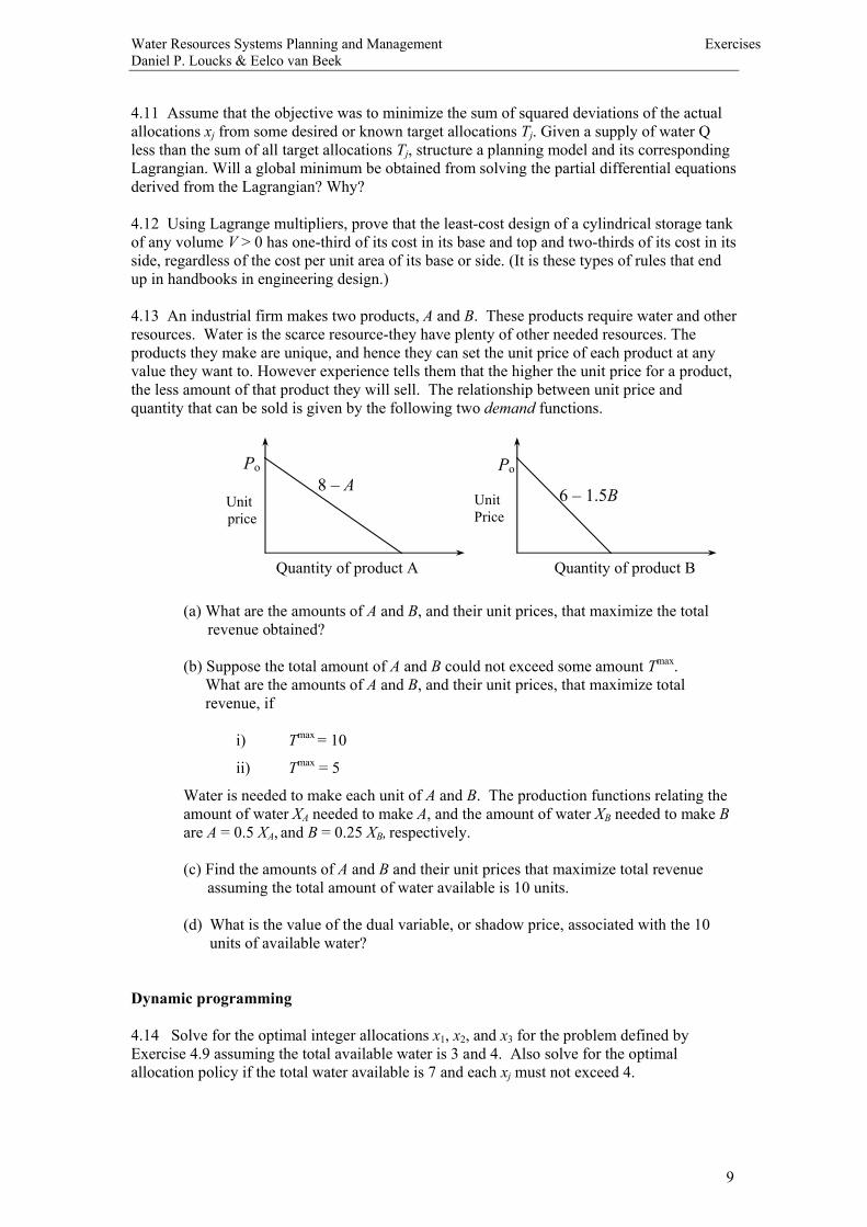
4.11 Assume that the objective was to minimize the sum of squared deviations of the actualallocations xj from some desired or known target allocations Tj. Given a supply of water Qless than the sum of all target allocations Tj, structure a planning model and its correspondingLagrangian. Will a global minimum be obtained from solving the partial differential equationsderived from the Lagrangian? Why?
4.12 Using Lagrange multipliers, prove that the leastcost design of a cylindrical storage tankof any volume V > 0 has onethird of its cost in its base and top and twothirds of its cost in itsside, regardless of the cost per unit area of its base or side. (It is these types of rules that endup in handbooks in engineering design.)
4.13 An industrial firm makes two products, A and B. These products require water and otherresources. Water is the scarce resourcethey have plenty of other needed resources. Theproducts they make are unique, and hence they can set the unit price of each product at anyvalue they want to. However experience tells them that the higher the unit price for a product,the less amount of that product they will sell. The relationship between unit price andquantity that can be sold is given by the following two demand functions.
(a) What are the amounts of A and B, and their unit prices, that maximize the total revenue obtained?
(b) Suppose the total amount of A and B could not exceed some amount Tmax.What are the amounts of A and B, and their unit prices, that maximize totalrevenue, if
i) Tmax = 10
ii) Tmax = 5
Water is needed to make each unit of A and B. The production functions relating theamount of water XA needed to make A, and the amount of water XB needed to make Bare A = 0.5 XA, and B = 0.25 XB, respectively.
(c) Find the amounts of A and B and their unit prices that maximize total revenue assuming the total amount of water available is 10 units.
(d) What is the value of the dual variable, or shadow price, associated with the 10units of available water?
Dynamic programming
4.14 Solve for the optimal integer allocations x1, x2, and x3 for the problem defined byExercise 4.9 assuming the total available water is 3 and 4. Also solve for the optimalallocation policy if the total water available is 7 and each xj must not exceed 4.
Quantity of product A Quantity of product B
Po
Unit price
Po
Unit Price
8 –A 6 – 1.5B
Water Resources Systems Planning and Management ExercisesDaniel P. Loucks & Eelco van Beek
10
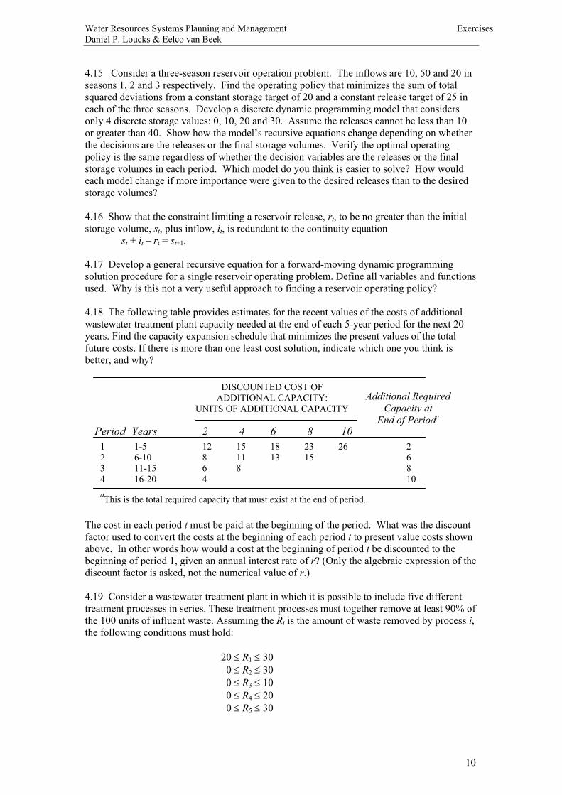
4.15 Consider a threeseason reservoir operation problem. The inflows are 10, 50 and 20 inseasons 1, 2 and 3 respectively. Find the operating policy that minimizes the sum of totalsquared deviations from a constant storage target of 20 and a constant release target of 25 ineach of the three seasons. Develop a discrete dynamic programming model that considersonly 4 discrete storage values: 0, 10, 20 and 30. Assume the releases cannot be less than 10or greater than 40. Show how the model’s recursive equations change depending on whetherthe decisions are the releases or the final storage volumes. Verify the optimal operatingpolicy is the same regardless of whether the decision variables are the releases or the finalstorage volumes in each period. Which model do you think is easier to solve? How wouldeach model change if more importance were given to the desired releases than to the desiredstorage volumes?
4.16 Show that the constraint limiting a reservoir release, rt, to be no greater than the initialstorage volume, st, plus inflow, it, is redundant to the continuity equation
st + it –rt = st+1.
4.17 Develop a general recursive equation for a forwardmoving dynamic programmingsolution procedure for a single reservoir operating problem. Define all variables and functionsused. Why is this not a very useful approach to finding a reservoir operating policy?
4.18 The following table provides estimates for the recent values of the costs of additionalwastewater treatment plant capacity needed at the end of each 5year period for the next 20years. Find the capacity expansion schedule that minimizes the present values of the totalfuture costs. If there is more than one least cost solution, indicate which one you think isbetter, and why?
The cost in each period t must be paid at the beginning of the period. What was the discountfactor used to convert the costs at the beginning of each period t to present value costs shownabove. In other words how would a cost at the beginning of period t be discounted to thebeginning of period 1, given an annual interest rate of r? (Only the algebraic expression of thediscount factor is asked, not the numerical value of r.)
4.19 Consider a wastewater treatment plant in which it is possible to include five differenttreatment processes in series. These treatment processes must together remove at least 90% ofthe 100 units of influent waste. Assuming the Ri is the amount of waste removed by process i,the following conditions must hold:
20 £ R1 £ 30 0 £ R2 £ 30 0 £ R3 £ 10 0 £ R4 £ 20 0 £ R5 £ 30
DISCOUNTED COST OFADDITIONAL CAPACITY:
UNITS OF ADDITIONAL CAPACITY
Period Years 2 4 6 8 101 15 12 15 18 23 26 22 610 8 11 13 15 63 1115 6 8 84 1620 4 10
Additional RequiredCapacity at
End of Perioda
aThis is the total required capacity that must exist at the end of period.
Water Resources Systems Planning and Management ExercisesDaniel P. Loucks & Eelco van Beek
11
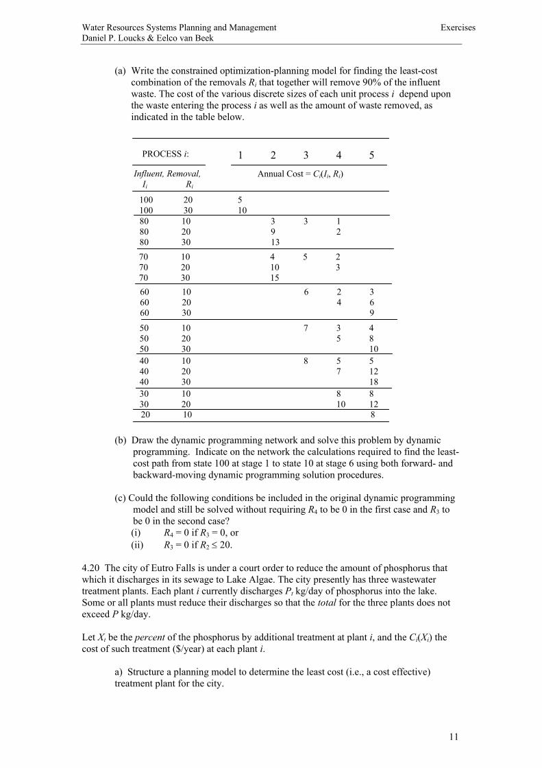
(a) Write the constrained optimizationplanning model for finding the leastcostcombination of the removals Ri that together will remove 90% of the influentwaste. The cost of the various discrete sizes of each unit process i depend uponthe waste entering the process i as well as the amount of waste removed, asindicated in the table below.
(b) Draw the dynamic programming network and solve this problem by dynamicprogramming. Indicate on the network the calculations required to find the leastcost path from state 100 at stage 1 to state 10 at stage 6 using both forward andbackwardmoving dynamic programming solution procedures.
(c) Could the following conditions be included in the original dynamic programmingmodel and still be solved without requiring R4 to be 0 in the first case and R3 tobe 0 in the second case?(i) R4 = 0 if R3 = 0, or(ii) R3 = 0 if R2 £ 20.
4.20 The city of Eutro Falls is under a court order to reduce the amount of phosphorus thatwhich it discharges in its sewage to Lake Algae. The city presently has three wastewatertreatment plants. Each plant i currently discharges Pt kg/day of phosphorus into the lake.Some or all plants must reduce their discharges so that the total for the three plants does notexceed P kg/day.
Let Xt be the percent of the phosphorus by additional treatment at plant i, and the Ci(Xi) thecost of such treatment ($/year) at each plant i.
a) Structure a planning model to determine the least cost (i.e., a cost effective)treatment plant for the city.
PROCESS i:
Influent, Removal, Ii Ri
100 20 5100 30 10
1 2 3 4 5
Annual Cost = Ci(Ii, Ri)
80 10 3 3 180 20 9 280 30 1370 10 4 5 270 20 10 370 30 1560 10 6 2 360 20 4 660 30 9
50 10 7 3 450 20 5 850 30 1040 10 8 5 540 20 7 1240 30 1830 10 8 830 20 10 1220 10 8

Water Resources Systems Planning and Management ExercisesDaniel P. Loucks & Eelco van Beek
12
b) Restructure the model for the solution by dynamic programming. Define thestages, states, decision variables, and the recursive equation for each stage.
c) Now assume P1 = 20; P2 = 15; P3 = 25; and P = 20. Make up some cost data andcheck the model if it works.
4.21 Find (draw) a rule curve for operating a single reservoir that maximizes the sum of thebenefits for flood control, recreation, water supply and hydropower. Assume the averageinflows in four seasons of a year are 40, 80 60, 20, and the active reservoir capacity is 100.For an average storage S and for a release of R in a season, the hydropower benefits are 2times the square root of the product of S and R, 2(S R)0.5 and the water supply benefits are3R0.7 in each season. The recreation benefits are 40(70S)2 in the third season. The floodcontrol benefits are 20 – (40 –S)2 in the second season. Specify the dynamic programmingrecursion equations you are using to solve the problem.
4.22 How would the model defined in Exercise 4.21 change if there were a water userupstream of this reservoir and you were to find the best water allocation policy for that user,assuming known benefits associated with these allocations that are to be included in theoverall maximum benefits objective function?
4.23 Suppose there are four water users along a river who benefit from receiving water. Eachhas a water target, i.e., each expects and plans for a specified amount. These known watertargets are W(1), W(2), W(3), and W(4) for the four users respectively. Show how dynamicprogramming can be used to find two allocation policies. One is to be based on minimizingthe maximum deficit deviation from any target allocation. The other is to be based onminimizing the maximum percentage deficit from any target allocation.
424 An industrial firm makes two products, A and B. These products require water andother resources. Water is the scarce resourcethey have plenty of other needed resources. Theproducts they make are unique, and hence they can set the unit price of each product at anyvalue they want to. However experience tells them that the higher the unit price for a product,the less amount of that product they will sell. The relationship between unit price andquantity that can be sold is given by the following two demand functions.
(a) What are the amounts of A and B, and their unit prices, that maximize the totalrevenue that can be obtained? (You can use calculus to solve this problem if youwish.)
(b) Suppose the total amount of A and B could not exceed some amount Tmax.What are the amounts of A and B, and their unit prices, that maximize totalrevenue, if
iii) Tmax = 10
iv) Tmax = 5
Quantity of product A Quantity of product B
Po
Unit price
Po
Unit Price
8 –A 6 – 1.5B

Water Resources Systems Planning and Management ExercisesDaniel P. Loucks & Eelco van Beek
13
Water is needed to make each unit of A and B. The production functions relating theamount of water XA needed to make A, and the amount of water XB needed to make Bare A = 0.5 XA, and B = 0.25 XB, respectively.
(c) Find the amounts of A and B and their unit prices that maximize total revenueassuming the total amount of water available is 10 units. Use discrete dynamicprogramming, both forward and backwardmoving algorithms. You can assumeinteger values of each water allocation X for this exercise. Show your work on anetwork. For the backward moving algorithm, also show your work using tablesshowing the state, Si, the possible decision variables XA and XB and their values, thebest decision, and the best value, Fi(Si), associated with the best decision.
Gradient “Hillclimbing” methods
4.25 Solve Exercise 4.24(b) using hillclimbing techniques and assuming discrete integervalues and Tmax = 5. For example, which product would you produce if you could make only1 unit of either A or B? If you could make another unit of A or B, which would you make?Continue this process up to 5 units of products A and/or B.
Linear and nonlinear programming
4.26 Consider the industrial firm that makes two products A and B as described in Exercise4.24(b). Using Lingo (or any other program you wish):
(a) Find the amounts of A and B and their unit prices that maximize total revenue assuming the total amount of water available is 10 units.
(b) What is the value of the dual variable, or shadow price, associated with the 10units of available water?
(c) Suppose the demand functions are not really certain. How sensitive are theallocations of water to the parameter values in those functions? How sensitiveare the allocations to the parameter values 0.5 and 0.25 in the productionfunctions?
4.27 Assume that there are m industries or municipalities adjacent to a river, which dischargetheir wastes into the river. Denote the discharge sites by the subscript i and let Wi be the kg ofwaste discharged into the river each day at those sites i. To improve the quality downstream,wastewater treatment plants may be required at each site i. Let xi be the fraction of wasteremoved by treatment at each site i. Develop a model for estimating how much waste isremoval is required at each site to maintain acceptable water quality in the river at a minimumtotal cost. Use the following additional notation:
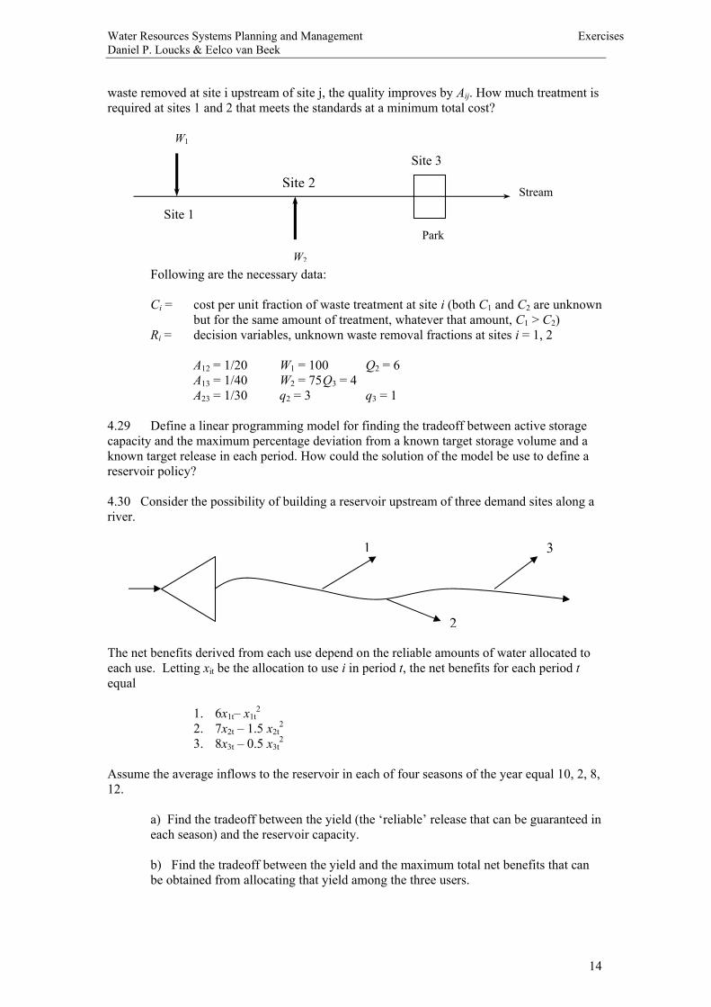
aij = decrease in quality at site j per unit of waste discharged at site iqj = quality at site j that would result if all controlled upstream discharges wereeliminated (i.e., W1 = W2 = 0)Qj = minimum acceptable quality at site jCi = cost per unit (fraction) of waste removed at site i
4.28 Assume that there are two sites along a stream, i = 1, 2, at which waste (BOD) isdischarged. Currently, without any wastewater treatment, the quality (DO), q2 and q3, at eachof sites 2 and 3 is less than the minimum desired, Q2 and Q3, respectively. For each unit of
Water Resources Systems Planning and Management ExercisesDaniel P. Loucks & Eelco van Beek
14
waste removed at site i upstream of site j, the quality improves by Aij. How much treatment isrequired at sites 1 and 2 that meets the standards at a minimum total cost?
Following are the necessary data:
Ci = cost per unit fraction of waste treatment at site i (both C1 and C2 are unknownbut for the same amount of treatment, whatever that amount, C1 > C2)
Ri = decision variables, unknown waste removal fractions at sites i = 1, 2
A12 = 1/20 W1 = 100 Q2 = 6A13 = 1/40 W2 = 75Q3 = 4A23 = 1/30 q2 = 3 q3 = 1
4.29 Define a linear programming model for finding the tradeoff between active storagecapacity and the maximum percentage deviation from a known target storage volume and aknown target release in each period. How could the solution of the model be use to define areservoir policy?
4.30 Consider the possibility of building a reservoir upstream of three demand sites along ariver.
The net benefits derived from each use depend on the reliable amounts of water allocated toeach use. Letting xit be the allocation to use i in period t, the net benefits for each period tequal
1. 6x1t–x1t2
2. 7x2t – 1.5 x2t2
3. 8x3t – 0.5 x3t2
Assume the average inflows to the reservoir in each of four seasons of the year equal 10, 2, 8,12.
a) Find the tradeoff between the yield (the ‘reliable’ release that can be guaranteed ineach season) and the reservoir capacity.
b) Find the tradeoff between the yield and the maximum total net benefits that canbe obtained from allocating that yield among the three users.
Site 1
Site 2Site 3
Park
W1
W2
Stream
1
2
3

Water Resources Systems Planning and Management ExercisesDaniel P. Loucks & Eelco van Beek
15
c) Find the tradeoff between the reservoir capacity and the total net benefits one canobtain from allocating the total releases, not just the reliable yield, to the downstreamusers.
d) Assuming a reservoir capacity of 5, and dividing the release into integerincrements of 2 (i.e., 2, 4, 6 and 8), using linear programming, find the optimaloperating policy. Assume the maximum release cannot exceed 8, and the minimumrelease cannot be less than 2. How does this solution differ from that obtained usingDP?
e) If you were maximizing the total net benefit obtained from the three users and ifthe water available to allocate to the three users were 15 in a particular time period,what would be the value of the Lagrange multiplier or dual variable associated withthe constraint that you cannot allocate more than 15 to the three uses?
f) There is the possibility of obtaining recreational benefits in seasons 2 and 3 fromreservoir storage. No recreational benefits can occur in seasons 1 and 4. To obtainthese benefits facilities must be built, and the question is at what elevation (storagevolume) should they be built. This is called the recreational storage volume target.Recreational benefits in each recreation season equal 8 per unit of storage target if theactual storage equals the storage target. If the actual storage is less than the target thelosses are 12 per unit deficit – the difference between the target and actual storagevolumes. If the actual storage volume is greater than the target volume the losses are4 per unit excess. What is the reservoir capacity and recreation storage target thatmaximizes the annual total net benefits obtained from downstream allocations andrecreation in the reservoir less the annual cost of the reservoir, 3K1.2, where K is thereservoir capacity?
g) In (f) above, suppose the allocation benefits and net recreation benefits weregiven weights indicating their relative importance. What happens to the relationshipbetween capacity K and recreation target Ts as the total allocation benefits are given agreater weight in comparison to recreation net benefits?
4.31 Using the network representation of the wastewater treatment plant design problemdefined in Exercise 4.19, write a linear programming model for defining the leastcostsequence of unit treatment process (i.e., the leastcost path through the network). [Hint: Leteach decision variable xij indicate whether or not the link between nodes (or states) i and jconnecting two successive stages is on the leastcost or optimal path. The constraints for eachnode must ensure that what enters the node must also leave the node.]
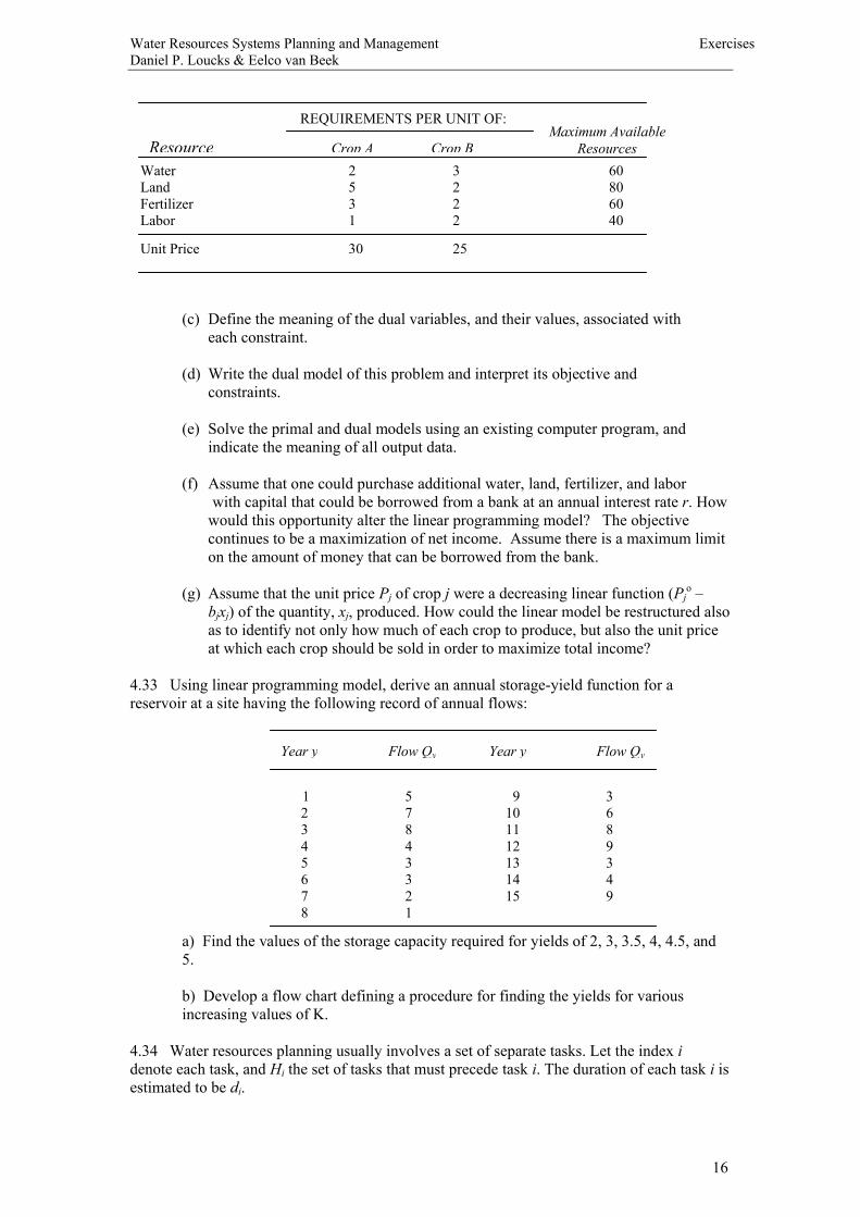
4.32 Two types of crops can be grown in particular irrigation area each year. Each unitquantity of crop A can be sold for a price PA and requires WA units of water, LA units of land,FA units of fertilizer, and HA units of labor. Similarly, crop B can be sold at a unit price of PBand requires WB, LB, FB and HB units of water, land, fertilizer, and labor, respectively, per unitof crop. Assume that the available quantities of water, land, fertilizer, and labor are known,and equal W, L, F, and H, respectively.
(a) Structure a linear programming model for estimating the quantities of each of thetwo crops that should be produced in order to maximize total income.
(b) Solve the problem graphically, using the following data:
Water Resources Systems Planning and Management ExercisesDaniel P. Loucks & Eelco van Beek
16
(c) Define the meaning of the dual variables, and their values, associated witheach constraint.
(d) Write the dual model of this problem and interpret its objective andconstraints.
(e) Solve the primal and dual models using an existing computer program, andindicate the meaning of all output data.
(f) Assume that one could purchase additional water, land, fertilizer, and laborwith capital that could be borrowed from a bank at an annual interest rate r. How
would this opportunity alter the linear programming model? The objectivecontinues to be a maximization of net income. Assume there is a maximum limiton the amount of money that can be borrowed from the bank.
(g) Assume that the unit price Pj of crop j were a decreasing linear function (Pjo –
bjxj) of the quantity, xj, produced. How could the linear model be restructured alsoas to identify not only how much of each crop to produce, but also the unit priceat which each crop should be sold in order to maximize total income?
4.33 Using linear programming model, derive an annual storageyield function for areservoir at a site having the following record of annual flows:
a) Find the values of the storage capacity required for yields of 2, 3, 3.5, 4, 4.5, and5.
b) Develop a flow chart defining a procedure for finding the yields for variousincreasing values of K.
4.34 Water resources planning usually involves a set of separate tasks. Let the index idenote each task, and Hi the set of tasks that must precede task i. The duration of each task i isestimated to be di.
REQUIREMENTS PER UNIT OF:
Resource Crop A Crop BWater 2 3 60Land 5 2 80Fertilizer 3 2 60Labor 1 2 40
10
Maximum AvailableResources
Unit Price 30 25
Year y Flow Qy Year y Flow Qy
1 5 9 3 2 7 10 6 3 8 11 8 4 4 12 9 5 3 13 3 6 3 14 4 7 2 15 9 8 1

Water Resources Systems Planning and Management ExercisesDaniel P. Loucks & Eelco van Beek
17
a) Develop a linear programming model to identify the starting times of tasks thatmaximizes the time, T, required to complete the total planning project.
b) Apply the general model to the following planning project:
Task A: Determine planning objectives and stakeholder interests. Duration: 4months
Task B: Determine structural and nonstructural alternatives that willinfluence objectives. Duration: 1 month.
Task C: Develop an optimization model for preliminary screening ofalternatives and for estimating tradeoffs among objectives. Duration:1 month.
Task D: Identify data requirements and collect data. Duration: 2 months.Task E: Develop a data management system for the project. Duration: 3
months.Task F: Develop an interactive shared vision simulation model with the
stakeholders.Duration: 2 Months.
Task G: Work with stakeholders in an effort to come to a consensus (a sharedvision) of the best plan. Duration: 4 months.
Task H: Prepare, present and submit a report. Duration: 2 months.
4.35 In Exercise 4.34 suppose the project is penalized if its completion time exceeds a targetT. The difference between 14 months and T months is D, and the penalty is P(D). You couldreduce the time it takes to complete task E by one month at a cost of $200, and by two monthsat a cost of $500. Similarly, suppose the cost of task A could be reduced by a month at a costof $600 and two months at a cost of $1400. Construct a model to find the most economicalproject completion time. Next modify the linear programming model to find the minimumtotal added cost if the total project time is to be reduced by 1 or 2 months. What is that addedcost and for which tasks?
4.36 Solve the reservoir operation problem described in Exercise 4.15 using linearprogramming. If the reservoir capacity is unknown, show how a cost function (that includesfixed costs and economies of scale) for the reservoir capacity could be included in the linearprogramming model.
4.37 An upstream reservoir could be built to serve two downstream users. Each user has aconstant water demand target. The first user’s target is 30; the second user’s target is 50.These targets apply to each of 6 withinyear seasons. Find the tradeoff between the requiredreservoir capacity and maximum deficit to any user at any time, for an average year. The
A
E
B
C
D
F
G H
Water Resources Systems Planning and Management ExercisesDaniel P. Loucks & Eelco van Beek
18
average flows into the reservoir in each of the six successive seasons are: 40, 80, 100, 130, 70,50.
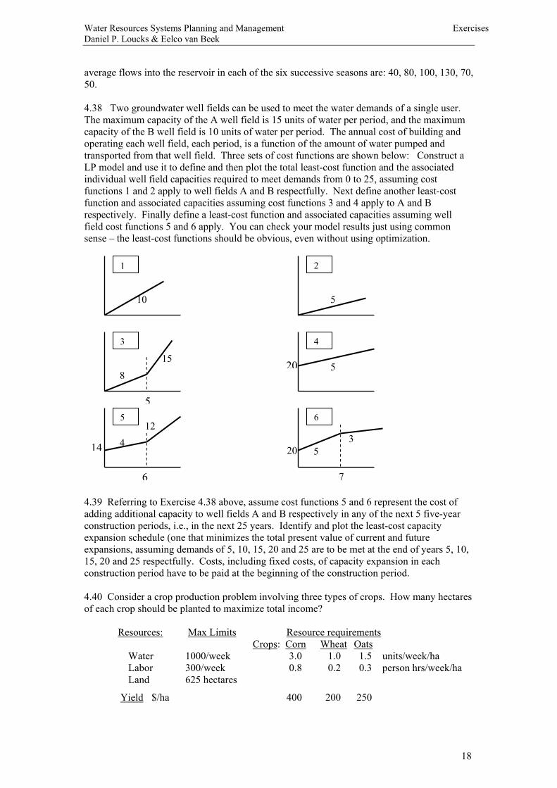
4.38 Two groundwater well fields can be used to meet the water demands of a single user.The maximum capacity of the A well field is 15 units of water per period, and the maximumcapacity of the B well field is 10 units of water per period. The annual cost of building andoperating each well field, each period, is a function of the amount of water pumped andtransported from that well field. Three sets of cost functions are shown below: Construct aLP model and use it to define and then plot the total leastcost function and the associatedindividual well field capacities required to meet demands from 0 to 25, assuming costfunctions 1 and 2 apply to well fields A and B respectfully. Next define another leastcostfunction and associated capacities assuming cost functions 3 and 4 apply to A and Brespectively. Finally define a leastcost function and associated capacities assuming wellfield cost functions 5 and 6 apply. You can check your model results just using commonsense – the leastcost functions should be obvious, even without using optimization.
4.39 Referring to Exercise 4.38 above, assume cost functions 5 and 6 represent the cost ofadding additional capacity to well fields A and B respectively in any of the next 5 fiveyearconstruction periods, i.e., in the next 25 years. Identify and plot the leastcost capacityexpansion schedule (one that minimizes the total present value of current and futureexpansions, assuming demands of 5, 10, 15, 20 and 25 are to be met at the end of years 5, 10,15, 20 and 25 respectfully. Costs, including fixed costs, of capacity expansion in eachconstruction period have to be paid at the beginning of the construction period.
4.40 Consider a crop production problem involving three types of crops. How many hectaresof each crop should be planted to maximize total income?
Resources: Max Limits Resource requirementsCrops: Corn Wheat Oats
Water 1000/week 3.0 1.0 1.5 units/week/ha Labor 300/week 0.8 0.2 0.3 person hrs/week/ha Land 625 hectares
Yield $/ha 400 200 250
10 5
815
5
20 5
412
6
53
7
20
1 2
3 4
5 6
14

Water Resources Systems Planning and Management ExercisesDaniel P. Loucks & Eelco van Beek
19
Show a twodimensional graph that defines the optimal solution(s) among Corn, Wheat andOats.
4.41 Releases from a reservoir are used for water supply or for hydropower. The benefit perunit of water allocated to hydropower is BH and the benefit per unit of water allocated towater supply is BW. For any given release the difference between the allocations to the twouses cannot exceed 50% of the total amount of water available. Show graphically how todetermine the most profitable allocation of the water for some assumed values of Bh and Bw.From the graph identify which constraints are binding and what their “dual prices” mean (inwords).
4.42 Suppose there are four water users along a river who benefit from receiving water. Eachhas a known water target, i.e., each expects and plans for a specified amount. These knownwater targets are W1, W2, W3, and W4 for the four users respectively. Find two allocationpolicies. One is to be based on minimizing the maximum deficit deviation from any targetallocation. The other is to be based on minimizing the maximum percentage deficit from anytarget allocation.
Deficit allocations are allocations that are less than the target allocation. For example if atarget allocation is 30 and the actual allocation is 20, the deficit is 10. Water in excess of thetargets can remain in the river. The policies are to indicate what the allocations should be forany particular river flow Q. The policies can be expressed on a graph showing the amount ofQ on the horizontal axis, and each user’s allocation on the vertical axis.
Create the two optimization models that can be used to find the two policies and indicate howthey would be used to define the policies. What are the unknown variables and what are theknown variables? Specify the model in words as well as mathematically.
4.43 In Indonesia there exists a wet season followed by a dry season each year. In one area ofIndonesia all farmers within an irrigation district plant and grow rice during the wet season.This crop brings the farmer the largest income per hectare; thus they would all prefer tocontinue growing rice during the dry season. However, there is insufficient water during thedry season to irrigate all 5000 hectares of available irrigable land for rice production. Assumean available irrigation water supply of 32 ´ 106 m3 at the beginning of each dry season, and aminimum requirement of 7000 m3/ha for rice and 1800 m3/ha for the second crop.
(a) What proportion of the 5000 hectares should the irrigation district managerallocate for rice during the dry season each year, provided that all availablehectares must be given sufficient water for rice or the second crop?
(b) Suppose that crop production functions are available for the two crops, indicatingthe increase in yield per hectare per m3 of additional water, up to 10, 000 m3/hafor the second crop. Develop a model in which the water allocation per hectare,as well as the hectares allocated to each crop, is to be determined, assuming aspecified price or return per unit of yield of each crop. Under what conditionswould the solution of this model be the same as in part (a)?
4.44 Along the Nile River in Egypt, irrigation farming is practiced for the production ofcotton, maize, rice, sorghum, full and short berseem for animal production, wheat, barley,horsebeans, and winter and summer tomatoes. Cattle and buffalo are also produced, andtogether with the crops that require labor, water. Fertilizer, and land area (feddans). Farmtypes or management practices are fairly uniform, and hence in any analysis of irrigationpolicies in this region this distinction need not be made. Given the accompanying datadevelop a model for determining the tons of crops and numbers of animals to be grown that
Water Resources Systems Planning and Management ExercisesDaniel P. Loucks & Eelco van Beek
20
will maximize (a) net economic benefits based on Egyptian prices, and (b) net economicbenefits based on international prices. Identify all variables used in the model.
Known parameters:Ci = miscellaneous cost of land preparation per feddan
EiP = Egyptian price per 1000 tons of crop iI
iP = international price per 1000 tons of crop iv = value of meat and dairy production per animalg = annual labor cost per workerfP = cost of P fertilizer per tonfN = cost of N fertilizer per tonYi = yield of crop i, tons/feddan
= feddans serviced per animal= tons straw equivalent per ton of berseem carryover from winter to summer
rw = berseem requirements per animal in winterswh = straw yield from wheat, tons per feddansba = straw yield from barley, tons per feddanrs = straw requirements per animal in summer
Nim = N fertilizer required per feddan of crop iPim = P fertilizer required per feddan of crop i
lim = labor requirements per feddan in month m, mandayswim = water requirements per feddan in month m, 1000 m3
him = land requirements per month, fraction (1 = full month)
Required Constraints. (assume known resource limitations for labor, water, and land):(a) Summer and winter fodder (berseem) requirements for the animals.(b) Monthly labor limitations.(c) Monthly water limitations.(d) Land availability each month.(e) Minimum number of animals required for cultivation.(f) Upper bounds on summer and winter tomatoes (assume these are known).(g) Lower bounds on cotton areas (assume this is known).
Other possible constraints:(a) Crop balances.(b) Fertilizer balances.(c) Labor balance.(d) Land balance.
4.45 In Algeria there are two distinct cropping intensities, depending upon the availability ofwater. Consider a single crop that can be grown under intensive rotation or extensive rotationon a total of A hectares. Assume that the annual water requirements for the intensive rotationpolicy are 16000 m3 per hectare, and for the extensive rotation policy they 4000 m3 perhectare. The annual net production returns are 4000 and 2000 dinars, respectively. If the totalwater available is 320,000 m3, show that as the available land area A increases, the rotationpolicy that maximizes total net income changes from one that is totally intensive to one that isincreasingly extensive.
Would the same conclusion hold if instead of fixed net incomes of 4000 and 2000 dinars perhectares of intensive and extensive rotation, the net income depended on the quantity of cropproduced? Assuming that intensive rotation produces twice as much produced by extensiverotation, and that the net income per unit of crop Y is defined by the simple linear function 5 –

Water Resources Systems Planning and Management ExercisesDaniel P. Loucks & Eelco van Beek
21
0.05Y, develop and solve a linear programming model to determine the optimal rotationpolicies if A equals 20, 50, and 80. Need this net income or price function be linear to beincluded in a linear programming model?
4.46 Current stream quality is below desired minimum levels throughout the stream inspite of treatment at each of the treatment plant and discharge sites shown below.Currently effluent standards are not being met, and minimum desired streamflowconcentrations can be met by meeting effluent standards. All current wastewaterdischarges must undergo additional treatment. The issue is where additional treatment isto occur and how much.
Develop a model to identify costeffective options for meeting effluent standards whereever wastewater is discharged into the stream. The decisions variables include theamount of wastewater to treat at each site and then release to the river. Any wastewaterat any site that is not undergoing additional treatment can be piped to other sites.Identify other issues that could affect the eventual decision.
Assume known current wastewater flows at site i = qi.Additional treatment to meet effluent standards cost = ai + bi(Di)ciwhere Di is the total wastewater flow undergoing additional treatment at site i and ci < 1.Pipeline and pumping for each pipeline segment costs approximately ij + (qij)where qij is pipeline flow between adjacent sites i and j and < 1.
4.47 Consider the system shown below where a reservoir is upstream of three demandsites along a river.
The net benefits derived from each use depend on the reliable amounts of water allocatedto each use. Letting xit be the allocation to use i in period t, the net benefits for eachperiod t equal
1. 6x1t–x1t2
2. 7x2t – 1.5 x2t2
3. 8x3t – 0.5 x3t2

Water Resources Systems Planning and Management ExercisesDaniel P. Loucks & Eelco van Beek
22
Assume the average inflows to the reservoir in each of four seasons of the year equal 10,2, 8, 12 units per season and that the reservoir capacity is 5 volume units.
a) Find the optimal operating policy for this reservoir that maximizes the total (four season)allocation benefits for the users.b) Simulate the operation of the reservoir and the allocation policy and using RIBASIM orWEAP or other simulation program (see CD).

Water Resources Systems Planning and Management ExercisesDaniel P. Loucks & Eelco van Beek
23
Chapter 5 Fuzzy Optimization
5.1 An upstream reservoir serves as a recreation site for swimmers, wind surfers and boaters.It also serves as a flood storage reservoir in the second period. The reservoir’s releases can bediverted to an irrigation area. A wetland area further downstream receives the unallocatedportion of the reservoir release plus the return flow from the irrigation area. The irrigationreturn flow contains a salinity concentration that can damage the ecosystem.
a) Assume there exist recreation lake level targets, irrigation allocation targets, andwetland flow and salinity targets. The challenge is to determine the reservoir releases andirrigation allocations so as to ‘best’ meet these targets. This is the crisp’ problem.
b) Assume that the targets used in a) above are really fairly fuzzy. Derive fuzzymembership functions for these targets and solve for the ‘best’ reservoir release and allocationpolicy based on these fuzzy membership functions. This is the ‘fuzzy’ problem.
Data:Reservoir storage capacity: 30 mcm;During period 2 the flood storage capacity is 5 mcm.Irrigation return flow fraction: 0.3 (i.e., 30% of that diverted for irrigation);Salinity concentration of reservoir water: 1 ppt;Salinity concentration of irrigation return flow: 20 ppt;Reservoir average inflows for four seasons, respectively: 5, 50, 20, 10 mcm;
Targets for part a):Target maximum salinity concentration in wetland: 3 ppt;Target storage target for all seasons: 20 mcm;Minimum flow target in wetland in each season, respectively: 10, 20, 15, 15 mcm;Maximum flow target in wetland in each season, respectively: 20, 30, 25, 25 mcm;Target irrigation allocations: 0, 20, 15, 5 mcm;
a) Find the reservoir releases in each season that best meet the flow and salinitytargets in the system. This is the crisp problem.
b) Next create fuzzy membership functions to replace the targets and solve theproblem.

Water Resources Systems Planning and Management ExercisesDaniel P. Loucks & Eelco van Beek
24
Chapter 6 DataBased Models
6.1 Develop a flow chart showing how you would apply genetic algorithms to finding theparameters, aij, of a water quality prediction model, such as the one we have used to find theconcentration downstream of an upstream discharge site. This will be based on observedvalues of mass inputs, Wi, and concentrations, Cj, and flows, Qj, at site j.
Cj = Si Wi aij ) / Qj
The objective to be used for fitness is to minimize the sum of the differences betweenthe observed Cj and the computed Cj. To convert this to a maximization objectiveyou could use something like the following:
Max 1 / (1 + D)
Where D ³ (Cj obs –Cj calculated)D ³ (Cj calculated –Cj obs.)
6.2 Use the genetic algorithm program called GANLC to predict the parameter valuesasked for in problem 6.1, and then the artificial neural network ANN to obtain a predictorof downstream water quality based on the values of these parameters. Both GANLC andANN are contained on the attached CD. You may use the model and data presented inSection 5.2 of Chapter 4 if you wish.
6.3 Using a genetic algorithm program (for example the one called GANLC containedon the CD) find the allocations Xi that maximize the total benefits to the three water usersi along a stream, whose individual benefits are:
Use 1: 6 X1 X12
Use 2: 7 X2 X22
Use 3: 8 X3 X32
Assume the available stream flow is some known value (ranging from 0 to 20).
Determine the effect of different genetic algorithm parameter values on the ability to findthe best solution.
6.4 Consider the wastewater treatment problem illustrated in the drawing below.
The initial stream concentration just upstream of site 1 is 32. The maximumconcentration of the pollutant just upstream of site 2 is 20 mg/l (g/m3), and at site 3 it is25 mg/l. Assume the marginal cost per fraction (or percentage) of the waste loadremoved at site 1 is no less than that cost at site 2, regardless of the amount removed.
Using the genetic algorithm program GANLC (contained on the CD), or other suitablegenetic algorithm program, solve for the least cost wastewater treatment at sites 1 and 2that will satisfy the quality constraints at sites 2 and 3 respectively.
Water Resources Systems Planning and Management ExercisesDaniel P. Loucks & Eelco van Beek
25
Discuss the sensitivity of the GA parameter values in finding the best solution. You can getthe exact solution using LINGO as discussed in Section 5.3 in Chapter 4.
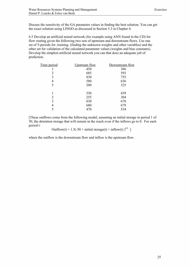
6.5 Develop an artificial neural network (for example using ANN found in the CD) forflow routing given the following two sets of upstream and downstream flows. Use oneset of 5periods for .training. (finding the unknown weights and other variables) and theother set for validation of the calculated parameter values (weights and bias constants).Develop the simplest artificial neural network you can that does an adequate job ofprediction.
Time period Upstream flow Downstream flow1 450 3662 685 5933 830 7554 580 6365 200 325
1 550 4392 255 3043 830 6784 680 6795 470 534
[These outflows come from the following model, assuming an initial storage in period 1 of50, the detention storage that will remain in the reach even if the inflows go to 0. For eachperiod t:
Outflow(t) = 1.5(50 + initial storage(t) + inflow(t) )0.9 ]
where the outflow is the downstream flow and inflow is the upstream flow.

Water Resources Systems Planning and Management ExercisesDaniel P. Loucks & Eelco van Beek
26
Chapter 7 Concepts in Probability, Statistics and StochasticModelling
7.1 Give an example of a water resources planning study with which you have somefamiliarity. Make a list of the basic information used in the study and the methods usedtransform that information into decisions, recommendations, and conclusions.
(a) Indicate the major sources of uncertainty and possible error in the basicinformation and in the transformation of that information into decisions,recommendations, and conclusions.
(b) In systems studies, sources of error and uncertainty are sometimes grouped intothree categories:
1. Uncertainty due to the natural variability of rainfall, temperature, andstream flows which affect a system’s operation.
2. Uncertainty due to errors made in the estimation of the models’parameters with a limited amount of data.
3. Uncertainty or errors introduced into the analysis because conceptualand/or mathematical models do not reflect the true nature of therelationships being described.
Indicate, if applicable, into which category each of the sources of error or uncertainty you have identified falls.
7.2 The following matrix displays the joint probabilities of different weather conditions andof different recreation benefit levels obtained from use of a reservoir in a state park:
(a) Compute the probabilities of recreation levels RB1, RB2, RB3, and of dry and wetweather.
(b) Compute the conditional probabilities P(wet½RB1), P(RB3½dry), and P(RB2½wet).
7.3 In flood protection planning, the 100year flood, which is an estimate of the quantile x0.99,is often used as the design flow. Assuming that the floods in different years are independentlydistributed:
(a) Show that the probability of at least one 100year flood in a 5year period is0.049.
(b) What is the probability of at least one 100year flood in a 100year period?(c) If floods at 1000 different sites occur independently, what is the probability of at
least one 100year flood at some site in any single year?
7.4 The price to be charged for water by an irrigation district has yet to be determined.Currently it appears as if there is as 60% probability that the price will be $10 per unit ofwater and a 40% probability that the price will be $5 per unit. The demand for water is
Weather RB1 RB2 RB2
Wet 0.10 0.20 0.10Dry 0.10 0.30 0.20
POSSIBLE RECREATION BENEFITS

Water Resources Systems Planning and Management ExercisesDaniel P. Loucks & Eelco van Beek
27
uncertain. The estimated probabilities of different demands given alternative prices are asfollows:
(a) What is the most likely value of future revenue from water sales?(b) What are the mean and variance of future water sales?(c) What is the median value and interquartile range of future water sales?(d) What price will maximize the revenue from the sale of water?
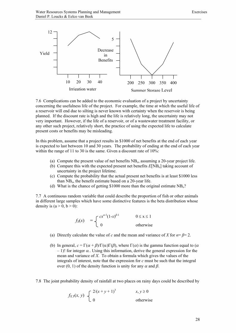
7.5 Plot the following data on possible recreation losses and irrigated agricultural yields.Show that use of the expected storage level or expected allocation underestimates theexpected value of the convex function describing reservoir losses while it overestimates theexpected value of the concave function describing crop yield. A concave function f(x) has theproperty that f(x) £ f(xo) + f’(xo)(x –xo) for any xo; prove that use of f(E[X]) will alwaysoverestimate the expected value of a concave function f(X) when X is a random variable.
Price / Quantity: 30 55 80 100 120
$ 5 0.00 0.15 0.30 0.35 0.20$ 10 0.20 0.30 0.40 0.10 0.00
Prob. of Quantity Demanded given Price
IrrigationWater
AllocationCrop
Yield/HectareProbability of
Allocation
10203040
6.510.012.011.0
0.200.300.300.20
Summer StorageLevel
Decrease inRecreation
Benefits
Probabilityof Storage
level
200250300350400
52014
0.100.200.400.200.10
Water Resources Systems Planning and Management ExercisesDaniel P. Loucks & Eelco van Beek
28
7.6 Complications can be added to the economic evaluation of a project by uncertaintyconcerning the usefulness life of the project. For example, the time at which the useful life ofa reservoir will end due to silting is never known with certainty when the reservoir is beingplanned. If the discount rate is high and the life is relatively long, the uncertainty may notvery important. However, if the life of a reservoir, or of a wastewater treatment facility, orany other such project, relatively short, the practice of using the expected life to calculatepresent costs or benefits may be misleading.
In this problem, assume that a project results in $1000 of net benefits at the end of each yearis expected to last between 10 and 30 years. The probability of ending at the end of each yearwithin the range of 11 to 30 is the same. Given a discount rate of 10%:
(a) Compute the present value of net benefits NBo, assuming a 20year project life.(b) Compare this with the expected present net benefits E[NBo] taking account of
uncertainty in the project lifetime.(c) Compute the probability that the actual present net benefits is at least $1000 less
than NBo, the benefit estimate based on a 20year life.(d) What is the chance of getting $1000 more than the original estimate NBo?
7.7 A continuous random variable that could describe the proportion of fish or other animalsin different large samples which have some distinctive features is the beta distribution whosedensity is (a > 0, b > 0):
cx 1(1x) 1 0 £ x £ 1
0 otherwise
(a) Directly calculate the value of c and the mean and variance of X for = = 2.
(b) In general, c = G(a + b)/G(a)G(b), where G(a) is the gamma function equal to (a– 1)! for integer a.. Using this information, derive the general expression for themean and variance of X. To obtain a formula which gives the values of theintegrals of interest, note that the expression for c must be such that the integralover (0, 1) of the density function is unity for any a and b.
7.8 The joint probability density of rainfall at two places on rainy days could be described by
2/(x + y + 1)3 x, y ³ 0
0 otherwise
12
10Irrigation water
20 30 40
Yield
200
Summer Storage Level250 300 350
5
Decreasein
Benefits
400
fX(x) =
fX,Y(x, y)

Water Resources Systems Planning and Management ExercisesDaniel P. Loucks & Eelco van Beek
29
Calculate and graph:(a) FXY(x, y), the joint distribution function of X and Y.(b) FY(y), the marginal cumulative distribution function of Y, and fY(y), the density
function of Y.(c) fY êX(y ê x), the conditional density function of Y given that X = x, and FY êX(y ê x),
the conditional cumulative distribution function of Y given that X = x (thecumulative distribution function is obtained by integrating the density function).
Show thatFY êX(y ê x = 0) > FY(y) for y > 0
Find a value of xo and yo for which
FY êX(yo ê xo) < FY(yo)
7.9 Let X and Y be two continuous independent random variables. Prove that
E[g(X)h(Y)] = E[g(X)]E[h(Y)]
for any two realvalued functions g and h. Then show that Cov(X, Y) = 0 if X and Y areindependent.
7.10 A frequent problem is that observations (X, Y) are taken on such quantities as flow andconcentration and then a derived quantity g(X, Y) such as mass flux is calculated. Given thatone has estimates of the standard deviations of the observations X and Y and their correlation,an estimate of the standard deviation of g(X, Y) is needed. Using a secondorder Taylor seriesexpansion for the mean of g(X, Y) as a function of its partial derivatives and of the means,variances, covariance of the X ad Y. Using a firstorder approximation of g(X, Y), obtained anestimates of the variances of g(X, Y) as a function of its partial derivatives and the momentsof X and Y. Note, the covariance of X and Y equals
E[(X –mX)(Y –mY)] = s2XY
7.11 A study of the behavior of water waves impinging upon and reflecting off a breakwaterlocated on a sloping beach was conducted in a small tank. The height (cresttotrough) of thewaves was measured a short distance from the wave generator and at several points along thebeach different distances from the breakwater were measured and their mean and standarderror recorded.
At which points were the wave heights significantly different from the height near wavegenerator assuming that errors were independent?
Location
Mean WaveHeight(cm)
StandardError of Mean
(cm)
Near wave generator1.9 cm from breakwater1.9 cm from breakwater1.9 cm from breakwater
3.324.422.593.26
0.060.090.090.06
Water Resources Systems Planning and Management ExercisesDaniel P. Loucks & Eelco van Beek
30
Of interest to the experimenter is the ratio of the wave heights near the breakwater to theinitial wave heights in the deep water. Using the results in Exercise 7.10, estimate thestandard error of this ratio at the three points assuming that errors made in measuring theheight of waves at the three points and near the wave generator are independent. At whichpoint does the ratio appear to be significantly different from 1.00?
Using the results of Exercise 7.10, show that the ratio of the mean wave heights is probably abiased estimate of the actual ratio. Does this bias appear to be important?
7.12 Derive Kirby’s bound, Equation 7.45, on the estimate of the coefficient of skewness bycomputing the sample estimates of the skewness of the most skewed sample it would bepossible to observe. Derive also the upper bound (n 1)1/2 for the estimate of the populationcoefficient of variation
xxn
when all the observations must be nonnegative.
7.13 The errors in the predictions of water quality models are sometimes described by thedouble exponential distribution whose density is
)exp(2
)( baa--= xxf ¥ < x <+ ¥
What are the maximum likelihood estimates of a and b? Note that
bb
-xdd
= 1 x > b
+1 x < b
Is there always a unique solution for b?
7.14 Derive the equations that one would need to solve to obtain maximum likelihoodestimates of the two parameters a and b of the gamma distribution. Note an analyticalexpression for dG(a)/da is not available so that a closed form expression for maximumlikelihood estimate of a is not available. What is the maximum likelihood estimate of b as afunction of the maximum likelihood estimates of a?
7.15 The logPearson TypeIII distribution is often used to model flood flows. If X has a logPearson TypeIII distribution then
Y = ln(X) –m
has a two parameter gamma distribution where em is the lower bound of X if b > 0 and em isthe upper bound of X if b < 0. The density function of Y can be written
)()exp()(
)()(1
ydyydyyfY bba
b a
-G
=-
0 < by < + ¥
Calculate the mean and variance of X in terms of a, b and m. Note that
E[Xr] = E[(exp(Y + m))r] = exp(rm) E[exp(rY)]

Water Resources Systems Planning and Management ExercisesDaniel P. Loucks & Eelco van Beek
31
To evaluate the required integrals remember that the constant terms in the definition of fY(y)ensure that the integral of this density function over the range of by must be unity for anyvalues of a and b so long as a > 0 and by > 0. For what values of r and b does the mean of Xfail to exist? How do the values of m, a and b affect the shape and scale of the distribution ofX?
7.16 When plotting observations to compare the empirical and fitted distributions ofstreamflows, or other variables, it is necessary to assign a cumulative probability to eachobservation. These are called plotting positions. As noted in the text, for the ith largestobservation Xi,
E[FX(Xi)] = i/(n + 1)
Thus the Weibull plotting position i/(n + 1) is one logical choice. Other commonly usedplotting positions are the Hazen plotting position (i –3/8)/(n + ¼). The plotting position (i –3/8)/(n + ¼) is a reasonable choice because its use provides a good approximation to theexpected value of Xi. In particular for standard normal variables
E[Xi] @ F1[(i –3/8)/(n + ¼)]
where F( × ) is the cumulative distribution function of a standard normal variable. While muchdebate centers on the appropriate plotting position to use to estimate pi = FX(Xi), often peoplefail to realize how imprecise all such estimates must be. Noting that
Var(pi) =)2()1(
)1(2 ++
--nn
ini,
contrast the difference between the estimates ip̂ of pi provided by these three plottingpositions and the standard deviation of pi. Provide a numerical example. What do youconclude?
7.17 The following data represent a sequence of annual flood flows, the maximum flow rateobserved each year, for the Sebou River at the Azib Soltane gaging station in Morocco.
Maximum Discharge Maximum DischargeDate (m3/s) Date (m3/s)
03/26/33 445 03/13/54 75012/11/33 1410 02/27/55 60311/17/34 475 04/08/56 88003/13/36 978 01/03/57 48512/18/36 461 12/15/58 81212/15/37 362 12/23/59 142004/08/39 530 01/16/60 409002/04/40 350 01/26/61 37602/21/41 1100 03/24/62 90402/25/42 980 01/07/63 412012/20/42 575 12/21/63 174002/29/44 694 03/02/65 97312/21/44 612 02/23/66 37812/24/45 540 10/11/66 82705/15/47 381 04/01/68 62605/11/48 334 02/28/69 317005/11/49 670 01/13/70 279001/01/50 769 04/04/71 113012/30/50 1570 01/18/72 43701/26/52 512 02/16/73 31201/20/53 613
Water Resources Systems Planning and Management ExercisesDaniel P. Loucks & Eelco van Beek
32
(a) Construct a histogram of the Sebou flood flow data to see what the flowdistribution looks like.
(b) Calculate the mean, variance, and sample skew. Based on Table 7.3, does thesample skew appear to be significantly different from zero?
(c) Fit a normal distribution to the data and use the KolmogorovSmirnov test todetermine if the fit is adequate. Draw a quantilequantile plot of the fitted
quantiles F1[(i –3/8)/(n + ¼)] versus the observed quantiles xi and include on thegraph the KolmogorovSmirnov bounds on each xi, as shown in Figures 7.2a and7.2b.
(d) Repeat part (c) using a twoparameter lognormal distribution.(e) Repeat part (c) using a threeparameter lognormal distribution. The Kolmogorov
Smirnov test is now approximate if applied to loge[Xi – ], where is calculatedusing Equation 7.81 or some other method of your choice.
(f) Repeat part (c) for two and three parameter versions of the gamma distribution.Again, the KolmogorovSmirnov test is approximate.
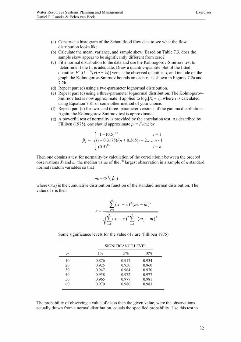
(g) A powerful test of normality is provided by the correlation test. As described byFilliben (1975), one should approximate pi = FX(xi) by
1 – (0.5)1/n i = 1ip̂ = (i – 0.3175)/(n + 0.365)i = 2,… , n 1
(0.5)1/n i = n
Then one obtains a test for normality by calculation of the correlation r between the orderedobservations Xi and mi the median value of the ith largest observation in a sample of n standardnormal random variables so that
mi = F1( ip̂ )where F(x) is the cumulative distribution function of the standard normal distribution. Thevalue of r is then
å å
å
= =
=
--
--=
n
ij
n
ii
n
iii
mmxx
mmxxr
1
2
1
2
1
22
)()(
)()(
Some significance levels for the value of r are (Filliben 1975)
The probability of observing a value of r less than the given value, were the observationsactually drawn from a normal distribution, equals the specified probability. Use this test to
n 1%
102030405060
SIGNIFICANCE LEVEL
5% 10%
0.8760.9250.9470.9580.9650.970
0.9170.9500.9640.9720.9770.980
0.9340.9600.9700.9770.9810.983
Water Resources Systems Planning and Management ExercisesDaniel P. Loucks & Eelco van Beek
33
determine whether a normal or twoparameter lognormal distribution provides an adequatemodel for these flows.
7.18 A small community is considering the immediate expansion of its wastewater treatmentfacilities so that the expanded facility can meet the current deficit of 0.25 MGD and theanticipated growth in demand over the next 25 years. Future growth is expected to result inthe need of an additional 0.75 MGD. The expected demand for capacity as a function of timeis
Demand = 0.25 MGD + G(1 –e0.23t)
where t is the time in years and G = 0.75 MGD. The initial capital costs and maintenance andoperating costs related to capital are $1.2 ´ 106 C0.70 where C is the plant capacity (MGD).Calculate the loss of economic efficiency LEE and the misrepresentation of minimal costs(MMC) that would result if a designer incorrectly assigned G a value of 0.563 or 0.938 (±25%) when determining the required capacity of the treatment plant. [Note: When evaluatingthe true cost of a nonoptimal design which provides insufficient capacity to meet demandover a 25year period, include the cost of building a second treatment plant; use an interestrate of 7% per year to calculate the present value of any subsequent expansions.] In thisproblem, how important is an error in G compared to an error in the elasticity of costs equal to0.70? One MGD, a million gallons per day, is equivalent to 0.0438 m3/s.
7.19 A municipal water utility is planning the expansion of their water acquisition systemover the next 50 years. The demand for water is expected to grow and is given by
D = 10t(1 – 0.006t)
where t is the time in years. It is expected that two pipelines will be installed along anacquired rightofway to bring water to the city from a distant reservoir. One pipe will beinstalled immediately and then a second pipe when the demand just equals the capacity C inyear t is
PV = (a + bCg)ert
wherea = 29.5b = 5.2g = 0.5r = 0.07/year
Using a 50year planning horizon, what is the capacity of the first pipe which minimizes thetotal present value of the construction of the two pipelines? When is the second pipe built? Ifa ± 25% error is made in estimating or r, what are the losses of economic efficiency (LEE)and the misrepresentation of minimal costs (MMC)? When finding the optimal decision witheach set of parameters, find the time of the second expansion to the nearest year; a computerprogram that finds the total present value of costs as a function of the time of the secondexpansion t for t = 1, … , 50 would be helpful. (A second pipe need not be built.)
7.20 A national planning agency for a small country must decide how to develop the waterresources of a region. Three development plans have been proposed, which are denoted d1, d2,and d3. Their respective costs are 200f, 100 f, and 100 f where f is a million farths, the nationalcurrency. The national benefits which are derived from the chosen development plan depend,in part, on the international market for the goods and agricultural commodities that would beproduced. Consider three possible international market outcomes, m1, m2, and m3. Thenational benefits if development plan 1 selected would be, receptively, 400, 290, 250. The

Water Resources Systems Planning and Management ExercisesDaniel P. Loucks & Eelco van Beek
34
national benefits from selection of plan 2 would be 350, 160, 120, while the benefits fromselection of plan 3 would be 250, 200, 160.
(a) Is any plan inferior or dominated?(b) If one felt that probabilities could not be assigned to m1, m2, and m3 but wished to
avoid poor outcomes, what would be an appropriate decision criterion, and why?Which decisions would be selected using this criterion?
(c) If Pr[m1]= 0.50 and Pr[m2] = Pr[m3] = 0.25, how would each of the expected netbenefits and expected regret criteria rank the decisions?
7.21 Show that if one has a choice between two water management plans yielding benefits Xand Y, where X is stochastically smaller than Y, then for any reasonable utility function, plan Yis preferred to X.
7.22 A reservoir system was simulated for 100 years and the average annual benefits andtheir variance was found to be
4.93B =2 3.23Bs =
The correlation of annual benefits was also calculated and is:
(a) Assume that r(l) = 0 for l > k, compute (using Equation 7.137) the standard errorof the calculated average benefits for k = 0, 1, 2, 3, 4, and 5. Also calculate thestandard error of the calculated benefits, assuming that annual benefits may bethought of as a stochastic process with a correlation structure rB(k) = [rB(1)]k.What is the effect of the correlation structure among the observed benefits on thestandard error of their average?
(b) At the 90% and 95% levels, which of the rk are significantly different from zero,assuming that rB(l) = 0 for l > k?
7.23 Replicated reservoir simulations using two operating policies produced the followingresults:
k012345
rk
1.0000.3890.2500.0620.0790.041
6.042
Replicate Policy 1
123456789
1011
BENEFITS
6.273.954.495.105.317.156.906.036.356.957.96
Policy 2
4.202.583.875.704.026.754.214.133.687.456.86
Mean, XiStandard deviation of values, sxi 1.217
4.8591.570

Water Resources Systems Planning and Management ExercisesDaniel P. Loucks & Eelco van Beek
35
(a) Construct a 90% confidence limits for each of the two means iX .(b) With what confidence interval can you state that Policy 1 produces higher
benefits than Policy 2 using the sign test and using the ttest?(c) If the corresponding replicate with each policy were independent, estimate with
what confidence one could have concluded that Policy 1 produces higher benefitswith the ttest.
7.24 Assume that annual streamflow at a gaging site have been grouped into three categoriesor states. State 1 is 5 to 15 m3/s, state 2 is 15 to 25 m3/s, and state 3 is 25 to 35 m3/s, and thesegrouping contain all the flows on records. The following transition probabilities have beencomputed from record:
(a) If the flow for the current year is between 15 and 25 m3/s, what is the probabilitythat the annual flow 2 years from now will be in the range 25 to 35 m3/s?
(b) What is the probability of a dry, an average, and a wet year many years fromnow?
7.25 A Markov chain model for the streamflows in two different seasons has the followingtransition probabilities
Calculate the steadystate probabilities of the flows in each interval in each season.
7.26 Can you modify the deterministic discrete DP reservoiroperating model to include theuncertainty, expressed as Pij
t, of the inflows, as in Exercise 7.25?
1j =
2 3Pij
1i = 2
3
0.50.30.1
0.30.30.5
0.20.40.4
STREAMFLOW next Season 2
STREAMFLOWIN SEASON 1 03 m3/s 36 m3/s ³ 6 m3/s
010 m3/s³ 10 m3/s
0.250.05
0.500.55
0.250.40
STREAMFLOW next Season 1
STREAMFLOWIN SEASON 2 010 m3/s ³ 10 m3/s
03 m3/s36 m3/s³ 6 m3/s
0.700.500.40
0.300.500.60
Water Resources Systems Planning and Management ExercisesDaniel P. Loucks & Eelco van Beek
36
(Hints: The operating policy would define the release (or final storage) in each season as afunction of not only the initial storage but also the inflow. If the inflow changes, so might therelease or final storage volume. Hence you need to discretize the inflows as well as thestorage volumes. Both storage and inflow are state variables. Assume for this model you canpredict with certainty the inflow in each period at the beginning of the period. So, each nodeof the network represents a known initial storage and inflow value. You cannot predict withcertainty the following period’s flows, only their probabilities. What does the network looklike now?
7.27 Assume that there exist two possible discrete flows Qit into a small reservoir in each oftwo periods t each year having probabilities Pit. Find the steadystate operating policy (releaseas a function of initial reservoir volumes and current period’s inflow) for the reservoir thatminimizes the expected sum of squared deviations from storage and release targets. Limit thestorage volumes to integer values that vary from 3 to 5. Assume a storage volume target of 4and a release target of 2 in each period t. (Assume only integer values of all states anddecision variables and that each period’s inflow is known at the beginning of the period.)Find the annual expected sum of squared deviations from the storage and release targets.
This is an application of Exercise 7.26 except the flow probabilities are independentof the previous flow.
7.28 Assume that the streamflow Q at a particular site has cumulative distribution functionFQ(q) = q/(1 + q) for q ³ 0. The withdrawal x at that location must satisfy a chance constraintof the form Pr[x ³ Q] £ 1 . Write the deterministic equivalent for each of the followingchance constraints:
Pr[x £ Q] ³ 0.90 Pr[x ³ Q] £ 0.80Pr[x £ Q] £ 0.95 Pr[x £ Q] £ 0.10Pr[x ³ Q] ³ 0.75
7.29 Assume that a potential water user can withdraw water from an unregulated stream, andthat the probability distribution function FQ() of the available streamflow Q is known.Calculate the value of the withdrawal target T that will maximize the expected net benefitsfrom the water’s use given the two shortrun benefit functions specified below.
(a) The benefits from streamflow Q when the target is T are
B(Q çT) =
where d > b > g. In this case, the optimal target T* can be expressed as a functionof P* = FQ(T) = Pr{Q T}, the probability that the random streamflow Q will beless than or equal to T. Prove that
P* = (b –g)/( d – g).
i = 1Period, t
1 2
13
24
FLOWS, Qit
i = 2 i = 10.170.29
PROBABILITIES, Pit
i = 2
0.830.71
Bo + bT + g(Q –T) Q ³ TBo + bT + d(Q –T) Q < T
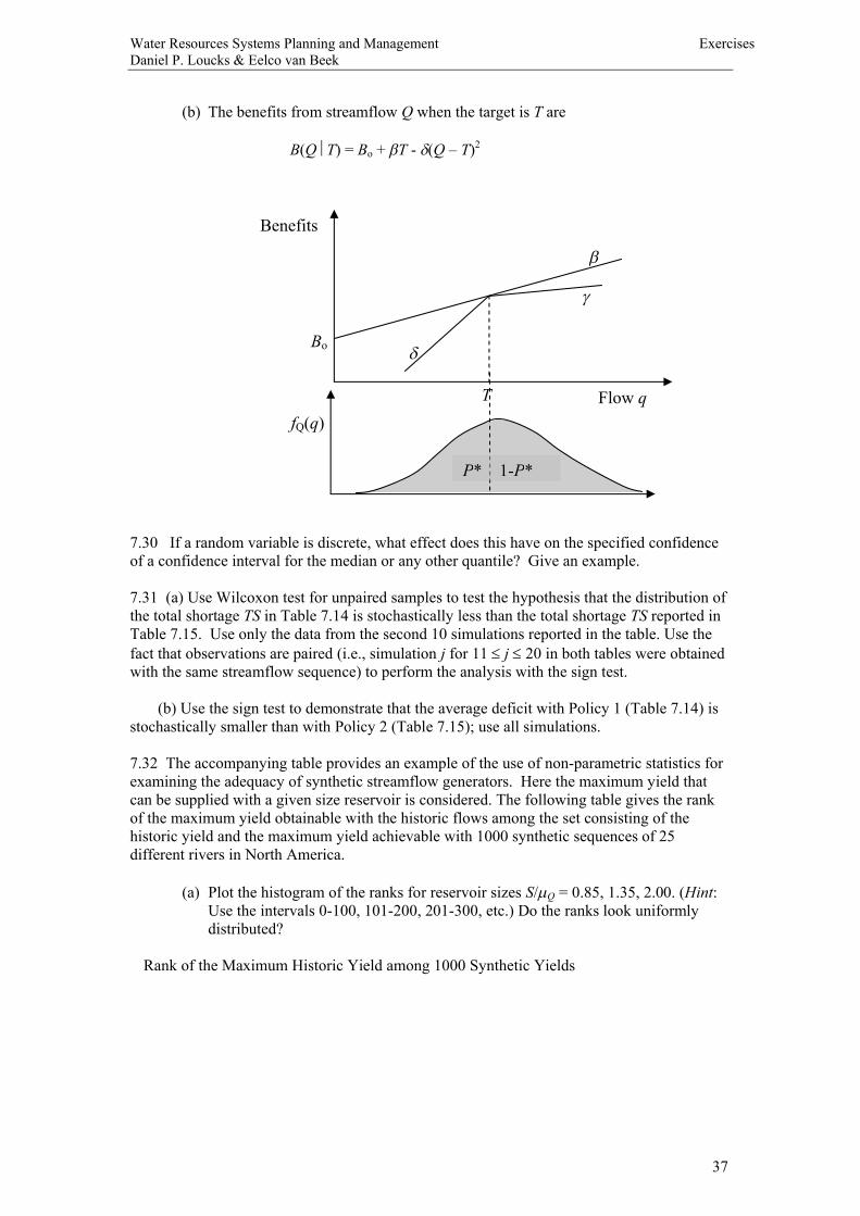
Water Resources Systems Planning and Management ExercisesDaniel P. Loucks & Eelco van Beek
37
(b) The benefits from streamflow Q when the target is T are
B(Q çT) = Bo + bT d(Q –T)2
7.30 If a random variable is discrete, what effect does this have on the specified confidenceof a confidence interval for the median or any other quantile? Give an example.
7.31 (a) Use Wilcoxon test for unpaired samples to test the hypothesis that the distribution ofthe total shortage TS in Table 7.14 is stochastically less than the total shortage TS reported inTable 7.15. Use only the data from the second 10 simulations reported in the table. Use thefact that observations are paired (i.e., simulation j for 11 £ j £ 20 in both tables were obtainedwith the same streamflow sequence) to perform the analysis with the sign test.
(b) Use the sign test to demonstrate that the average deficit with Policy 1 (Table 7.14) isstochastically smaller than with Policy 2 (Table 7.15); use all simulations.
7.32 The accompanying table provides an example of the use of nonparametric statistics forexamining the adequacy of synthetic streamflow generators. Here the maximum yield thatcan be supplied with a given size reservoir is considered. The following table gives the rankof the maximum yield obtainable with the historic flows among the set consisting of thehistoric yield and the maximum yield achievable with 1000 synthetic sequences of 25different rivers in North America.
(a) Plot the histogram of the ranks for reservoir sizes S/mQ = 0.85, 1.35, 2.00. (Hint:Use the intervals 0100, 101200, 201300, etc.) Do the ranks look uniformlydistributed?
Rank of the Maximum Historic Yield among 1000 Synthetic Yields
T
b
dBo
Benefits
Flow q
g
P* 1P*
fQ(q)

Water Resources Systems Planning and Management ExercisesDaniel P. Loucks & Eelco van Beek
38
(b) Do you think this streamflow generation model produces streamflows which areconsistent with the historic flows when one uses as a criterion the maximumpossible yield? Construct a statistical test to support your conclusion and showthat it does support your conclusion. (Idea: You might want to consider if it isequally likely that the rank of the historical yield is 500 and below 501 andabove. You could then use the binomial distribution to determine the significanceof the results.)
(c) Use the KolmogrovSmirnov test to check if the distribution of the yieldsobtainable with storage S/mQ = 1.35 is significantly different from uniform FU(u)= u for 0 £ u £ 1. How important do you feel this result is?
7.33 Section 7.3 dismisses the bias in nx2 for correlated X’s as unimportant to its variance.
(a) Calculate the approximate bias in nx2 for the cases corresponding to Table 7.10
and determine if this assertion is justified.(b) By numerically evaluating the bias and variance of nx
2, when n = 25, determine ifthe same result holds if rx(k) = 0.5(0.9)k, which is the autocorrelation function ofan ARMA (1, 1) process sometimes used to describe annual streamflow series.
7.34 Consider the crop irrigation problem in Exercise 4.31. For the given prices 30 and 25for crop A and B, the demand for each crop varies over time. Records of demands show forcrop A the demand ranges from 0 to 10 uniformly. There is an equal probability of that thedemand will be any value between 0 and 10. For crop B the demand ranges from 5 units to15 units, and the most likely demand is 10. At least 5 units and no more than 15 units of crop
RiverNumber 0.35
12345678910111213141516171819202122232425
NORMALIZED ACTIVE STORAGE, S/mQ
0.85 1.35
4729640236745376
4132743622402663547
5702864322
271295307
7618
126382
13620714627344292
36519112119066
43314545239223210217216244462481178
902127
23515684
19150254
2795129
14111873837935942197
266456291410332679778737910
12818312014141356
2738650
18860
562647380424112173260272532418801608878758
Source: A. I. McLeod and K. W. Hipel, Critical Drought Revisited,Paper presented at the international Symposium on Risk and Reliabilityin Water Resources, Waterloo, Ont., June 2628, 1978
2.00
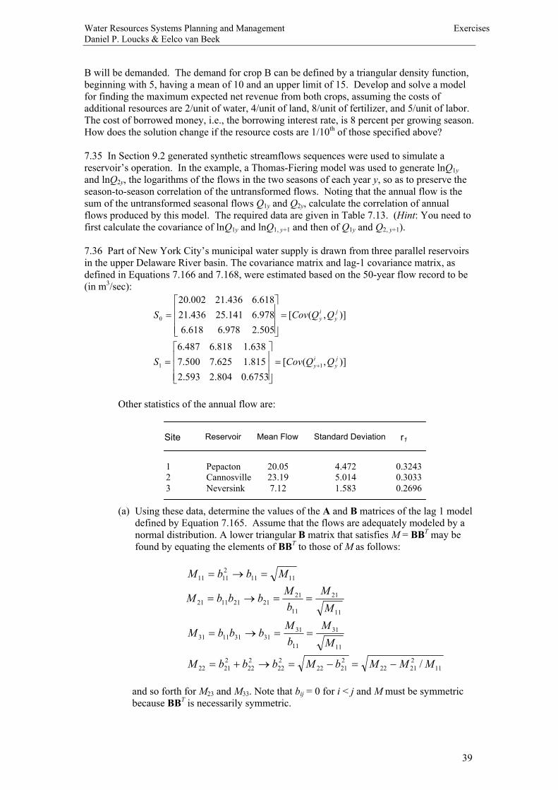
Water Resources Systems Planning and Management ExercisesDaniel P. Loucks & Eelco van Beek
39
B will be demanded. The demand for crop B can be defined by a triangular density function,beginning with 5, having a mean of 10 and an upper limit of 15. Develop and solve a modelfor finding the maximum expected net revenue from both crops, assuming the costs ofadditional resources are 2/unit of water, 4/unit of land, 8/unit of fertilizer, and 5/unit of labor.The cost of borrowed money, i.e., the borrowing interest rate, is 8 percent per growing season.How does the solution change if the resource costs are 1/10th of those specified above?
7.35 In Section 9.2 generated synthetic streamflows sequences were used to simulate areservoir’s operation. In the example, a ThomasFiering model was used to generate lnQ1yand lnQ2y, the logarithms of the flows in the two seasons of each year y, so as to preserve theseasontoseason correlation of the untransformed flows. Noting that the annual flow is thesum of the untransformed seasonal flows Q1y and Q2y, calculate the correlation of annualflows produced by this model. The required data are given in Table 7.13. (Hint: You need tofirst calculate the covariance of lnQ1y and lnQ1, y+1 and then of Q1y and Q2, y+1).
7.36 Part of New York City’s municipal water supply is drawn from three parallel reservoirsin the upper Delaware River basin. The covariance matrix and lag1 covariance matrix, asdefined in Equations 7.166 and 7.168, were estimated based on the 50year flow record to be(in m3/sec):
)],([505.2978.6618.6978.6141.25436.21618.6436.21002.20
0jy
iy QQCovS =
úúú
û
ù
êêê
ë
é=
)],([6753.0804.2593.2815.1625.7500.7638.1818.6487.6
11jy
iy QQCovS +=
úúú
û
ù
êêê
ë
é=
Other statistics of the annual flow are:
(a) Using these data, determine the values of the A and B matrices of the lag 1 modeldefined by Equation 7.165. Assume that the flows are adequately modeled by anormal distribution. A lower triangular B matrix that satisfies M = BBT may befound by equating the elements of BBT to those of M as follows:
11112
1111 MbbM =®=
11
21
11
2121211121 M
Mb
MbbbM ==®=
11
31
11
3131311131 M
MbM
bbbM ==®=
1122122
22122
222
222
22122 / MMMbMbbbM -=-=®+=
and so forth for M23 and M33. Note that bij = 0 for i < j and M must be symmetricbecause BBT is necessarily symmetric.
Site Reservoir Mean Flow Standard Deviation r1
123
PepactonCannosvilleNeversink
20.0523.197.12
4.4725.0141.583
0.32430.30330.2696
Water Resources Systems Planning and Management ExercisesDaniel P. Loucks & Eelco van Beek
40
(b) Determine A and BBT for the Markov model which would preserve the variancesand cross covariances of the flows at each site, but not necessarily the lag 1 crosscovariances of the flows. Calculate the lag 1 cross covariances of flows generatedwith your calculated A matrix.
(c) Assume that some model has been built to generate the total annual flow into thethree reservoirs. Construct and calculate the parameters of a disaggregation modelthat, given the total annual inflow to all three reservoirs, will generate annualinflows into each of the reservoirs preserving the variances and cross covariancesof the flows. [Hint: The necessary statistics of the total flows can be calculatedfrom those of the individual flows.]
7.37 Derive the variance of an ARMA (1, 1) process in terms of f1, q1, and sv2. [Hint:Multiply both sides of the equation to obtain a second. Be careful to remember which Vt’s areindependent of which Zt’s.]
7.38 The accompanying table presents a 60year flow record for the normalized flows of theGota River near SjotopVannersburg in Sweeden.
(a) Fit an autoregressive Markov model to the annual flow record.
(b) Using your model, generate a 50year synthetic flow record. Demonstrate themean, variance, and correlation of your generated flows deviate from thespecified values no more than would be expected as a result of sampling error.
(c) Calculate the autocorrelations and partial autocovariances of the annual flows fora reasonable number of lags. Calculate the standard errors of the calculatedvalues. Determine reasonable value of p and q for an ARMA (p, q) model of theflows. Determine the parameter values for the selected model.
Annual Flows, Gota River near SjotopVannersburg, Sweden1898 1.158 1918 0.948 1938 0.8921899 1.267 1919 0.907 1939 1.0201900 1.013 1920 0.991 1940 0.8691901 0.935 1921 0.994 1941 0.7721902 0.662 1922 0.701 1942 0.6061903 0.950 1923 0.692 1943 0.7391904 1.120 1924 1.086 1944 0.8131905 0.880 1925 1.306 1945 1.1731906 0.802 1926 0.895 1946 0.9161907 0.856 1927 1.149 1947 0.8801908 1.080 1928 1.297 1948 0.6011909 0.959 1929 1.168 1949 0.7201910 1.345 1930 1.218 1950 0.9551911 1.153 1931 1.209 1951 1.1861912 0.929 1932 0.974 1952 1.1401913 1.158 1933 0.834 1953 0.9921914 0.957 1934 0.638 1954 1.0481915 0.705 1935 0.991 1955 1.1231916 0.905 1936 1.198 1956 0.7741917 1.000 1937 1.091 1957 0.769
Source: V. M. Yevdjevich, Fluctuations of Wet and Dry Years, Part I,Hydrology Paper No. 1, Colorado State University, Fort Collins, Colo., 1963

Water Resources Systems Planning and Management ExercisesDaniel P. Loucks & Eelco van Beek
41
(d) Using the estimated model in (c), generate a 50year synthetic streamflow recordand demonstrate that the mean, variance, and show that first autocorrelations ofthe synthetic flows deviate from the modeled values by no more than would beexpected as a result of sampling error.
7.39 (a) Assume that one wanted to preserve the covariance matrices S0 and S1 of the flowsat several site Zy by using the multivariate or vector ARMA (0, 1) model
Zy+1 = AVy –BVy1
where Vy contains n independent standard normal random variables. What is the relationshipbetween the values of S0 and S1 and the matrices A and B?
(b) Derive estimates of the matrices A, B, and C of the multivariate AR(2) model
Zy+1 = AZy + BZy1 + CVy
using the covariance matrices S0, S1and S2.
7.40 Formulate a model for the generation of monthly flows. The generated monthly flowsshould have the same marginal distributions as were fitted to the observed flows of record andshould reproduce (i) the monthtomonth correlation of the flows, (ii) the monthtoseasoncorrelation between each monthly flow and the total flow the previous season, and (iii) themonthtoyear correlation between each monthly flow and the total 12month flow in theprevious year. Show how to estimate the model’s parameters. How many parameters doesyour model have? How are the values of the seasonal model? How do you think this modelcould be improved?

Water Resources Systems Planning and Management ExercisesDaniel P. Loucks & Eelco van Beek
42
Chapter 8 Modelling Uncertainty
8.1 Can you modify the deterministic discrete DP reservoiroperating model to include theuncertainty, expressed as Pij
t, of the inflows, as in Exercise 7.25?
(Hints: The operating policy would define the release (or final storage) in each season as afunction of not only the initial storage but also the inflow. If the inflow changes, so might therelease or final storage volume. Hence you need to discretize the inflows as well as thestorage volumes. Both storage and inflow are state variables. Assume for this model you canpredict with certainty the inflow in each period at the beginning of the period. So, each nodeof the network represents a known initial storage and inflow value. You cannot predict withcertainty the following period’s flows, only their probabilities. What does the network looklike now?
8.2 Assume that there exist two possible discrete flows Qit into a small reservoir in each oftwo periods t each year having probabilities Pit. Find the steadystate operating policy (releaseas a function of initial reservoir volumes and current period’s inflow) for the reservoir thatminimizes the expected sum of squared deviations from storage and release targets. Limit thestorage volumes to integer values that vary from 3 to 5. Assume a storage volume target of 4and a release target of 2 in each period t. (Assume only integer values of all states anddecision variables and that each period’s inflow is known at the beginning of the period.)Find the annual expected sum of squared deviations from the storage and release targets.
This is an application of Exercise 7.26 except the flow probabilities are independentof the previous flow.
8.3 Develop a linear model for defining the optimal joint probabilities of predefined discreteinitial storage volumes, discrete inflows, and discrete final storage volumes in a reservoir ineach period t. Let values of the index k represent the different discrete initial storagevolumes, Skt. Similarly, let the index i represent the inflows, Qit, and the index l represent thefinal storage volumes, Sl,t+1, in period t. Let the index j represent the discrete inflows, Qj,t+1,and m represent the discrete final storage volumes, Sm,t+2, in period t+1. Let PRkilt be theunknown joint probability of a discrete initial storage, Skt, an inflow, Qit, and a final storagevolume, Sl,t+1, in period t. It is also the probability of a release associated with a particularcombination of k, i, and l in period t. The objective is to maximize the expected net benefits,however measured. The net benefits associated with any combination represented by k, i, andl in period t is Bkilt. These net benefits and the conditional inflow probabilities. Pij
t =Pr{Qj,t+1|Qit}, are known. Show how the optimal operating policy can be determined once thevalues of the joint probabilities, PRkilt, are known.
The same policy can be found by DP. Develop a DP model to find the optimal operatingpolicy.
8.4 Referring to Exercise 8.3, instead of defining a final volume subscript l and m forcomputing joint probabilities PRkilt, assume that subscripts d and e were used to denotedifferent reservoir release volumes. How would the linear programming model developed be
i = 1Period, t
1 2
13
24
FLOWS, Qit
i = 2 i = 1
0.170.29
PROBABILITIES, Pit
i = 2
0.830.71

Water Resources Systems Planning and Management ExercisesDaniel P. Loucks & Eelco van Beek
43
altered to include d and e in place of l and m? How would the dynamic programmingrecursion equation be altered?
8.5 Given joint probabilities PRkilt found from Exercise 8.3, how would one derive theprobability distribution of reservoir releases and storage volumes in each period t?

Water Resources Systems Planning and Management ExercisesDaniel P. Loucks & Eelco van Beek
44
Chapter 9 Model Sensitivity and Uncertainty Analysis
9.1 Distinguish between sensitivity analysis and uncertainty analysis.
9.2 Consider the allocation model you have been using in previous chapters involving threewater consumers i. Allocations xi of water can be made from a given total amount Q to thethree consumers. The respective benefits are (6x1 –x1
2), (7x2 – 1.5x22) and (8x3 – 0.5x3
2).Discuss possible sources of uncertainty in model structure and model output, and identify anddisplay parameter sensitivity.
9.3 Discuss how model output uncertainty is impacted by both model input uncertainty aswell as parameter sensitivity.
9.4 In many water resources studies considerable attention is given to the uncertainty ofwater supplies (precipitation, streamflows, evaporation, infiltration, etc.) and much lessattention is given to the uncertainty of the management objectives, the costs and benefits ofinfrastructure, the political support associated with alternative possible decisions, and the like.Develop a simple water resources planning model involving the management of waterquantity and quality and show how these management objective uncertainties may actuallydominate the hydrologic uncertainties.
9.5 Perform a deterministic sensitivity analysis for the consumer 1 in Exercise 9.2. Considerthe three parameters, Q, 6 and 1; the later two numbers are the parameters of the benefitfunction. Low values of these three parameters are 3, 3, and 0.5 respectively. Most likelyvalues are 6, 6, and 1. High values are 12, 9, and 1.5. Display the results using a Paretochart, a tornado diagram, and a spider plot.
9.6 Referring to water allocation problem defined in Exercise 9.2, assume the availableamount of water Q is uncertain. Its cumulative probability distribution is defined by q/(6+q)for values q 0 of the random variable Q. The expected value of Q is 6. Perform anuncertainty analysis showing how to define, at least approximately:
· Estimating the mean and standard deviation of the outputs.· Estimating the probability the performance measure will exceed a specific
threshold.· Assigning a reliability level on a function of the outputs, e.g., the range of
function values that is likely to occur with some probability.· Describing the likelihood of different potential outputs of the system.
Show the application of Monte Carlo sampling and analysis, Latin hypercube sampling,generalized likelihood uncertainty estimation and factorial design methods.

Water Resources Systems Planning and Management ExercisesDaniel P. Loucks & Eelco van Beek
45
Chapter 10 Performance Criteria
10.1 Distinguish between multiple purposes and multiple objectives and give some examplesof complementary and conflicting purposes and objectives of water resources projects.
10.2 Assume that farmers’ demand for water q is a linear function a –bp of the price p,where a, b > 0. Calculate the farmers’ willingness to pay for a quantity of water q. If the costof delivering a quantity of water q is cq, c > 0, how much water should a public agencysupply to maximize willingness to pay minus total cost? If the local water district is ownedand operated by a private firm whose objective is to maximize profit, how much water wouldthey supply and how much would they earn? The farmers’ consumer surplus is theirwillingness to pay minus what they must pay for the resource. Compare the farmers’consumer surplus in two cases. Do the farmers loose more than the private firm gains bymoving from the social optimum to the point that maximize the firm’s profit? Illustrate theserelationships with a graph showing the demand curve and the unit cost c of water. Whichareas on the graph represent the firm’s profits and the farmers’ consumer surplus?
10.3 Consider the water allocation problem used in the earlier chapters of this book. Thereturns, Bi(Xi) from allocating Xi amount of water to each of three uses i are as follows, alongwith the optimal allocations from the point of view of each use.
( ) 21111 6 XXXB -= à 31 =optX and ( ) 911
max1 == optXBB
( ) 22222 5.17 XXXB -= à 372 =optX and ( ) 1814722
max2 == optXBB
( ) 23333 5.08 XXXB -= à 83 =optX and ( ) 3233
max3 == optXBB
Consider this a multiobjective problem. Instead of finding the best overall allocation thatmaximizes the total return assume the objectives are to maximize the returns from each user.
Show how the weighting, constraint, goal attainment, and goal programming methods can beused to identify the tradeoffs among each of the three objectives for any limiting total amountof water, for example 6.
10.4 Under what circumstances will the weighting and constraint methods fail to identifyefficient solutions?
10.5 A reservoir is planned for irrigation and low flow augmentation for water qualitycontrol. A storage volume of 6 ´ 106 m3 will be available for those two conflicting uses eachyear. The maximum irrigation demand (capacity) is 4 ´ 106 m3. Let X1 be the allocation ofwater to irrigation and X2 the allocation for downstream flow augmentation. Assume thatthere are two objectives, expressed as
Z1 = 4 X1 –X2Z2 = 2 X1 + 6X2
(a) Write the multiobjective planning model using a weighing approach and aconstraint approach.
(b) Define the efficient frontier. This requires a plot of the feasible combinations ofX1 and X2.
(c) Assume that various values are assigned to a weight W1 for Z1 whereas weight W2for Z2 is constant and equal to 1, verify the following solutions to the weighingmodel.
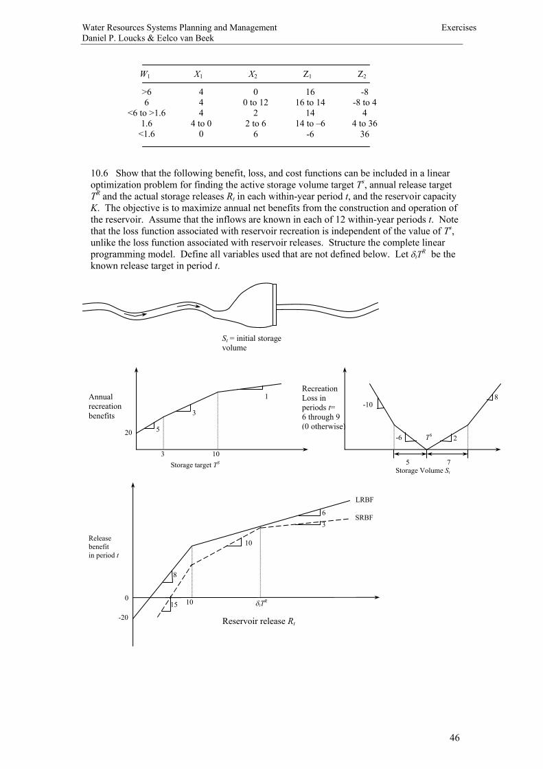
Water Resources Systems Planning and Management ExercisesDaniel P. Loucks & Eelco van Beek
46
10.6 Show that the following benefit, loss, and cost functions can be included in a linearoptimization problem for finding the active storage volume target Ts, annual release targetTR and the actual storage releases Rt in each withinyear period t, and the reservoir capacityK. The objective is to maximize annual net benefits from the construction and operation ofthe reservoir. Assume that the inflows are known in each of 12 withinyear periods t. Notethat the loss function associated with reservoir recreation is independent of the value of Ts,unlike the loss function associated with reservoir releases. Structure the complete linearprogramming model. Define all variables used that are not defined below. Let dtTR be theknown release target in period t.
3
8
10
20 Reservoir release Rt
Releasebenefitin period t
10
6
15 dtTR 0
LRBF
SRBF
W1 X1 X2 Z1 Z2
>66
<6 to >1.61.6
<1.6
444
4 to 00
00 to 12
22 to 6
6
1616 to 14
1414 to –6
6
88 to 4
44 to 36
36
St = initial storagevolume
3 10
20
Storage target TS
Annualrecreationbenefits 3
5
1
2
8
5Storage Volume St
RecreationLoss inperiods t=6 through 9(0 otherwise)
6
10
7
TS
Water Resources Systems Planning and Management ExercisesDaniel P. Loucks & Eelco van Beek
47
10.7 For the river basin shown, potential reservoirs exist at sites i = 1, 2, and 4 and adiversion can be constructed between sites 1 and 2. The cost Ci(Ki) of each reservoir i is afunction of its active storage capacity Ki. The cost of the diversion canal is Ci(Qi) where Qis the flow capacity of the canal. The cost of diverting a flow Qijt from site i to site j isCij(Qijt). The two users at sites 3 and 5 have known target allocations (demands) Tit in eachperiod t. The return flow from use 3 is 40% of that allocated to use 3. Construct a modelfor finding the least cost of meeting various percentages of the target demands. Assumethat the natural streamflows Qi
t at each site i in each period t, are known.
10.8 Suppose that there exist two polluters, A and B, who can provide additional treatment,XA and XB, at a cost of CA(XA) and CB(XB), respectively. Let WA and WB be the wasteproduced at sites A and B, and WA(1 –XA) and WB(1 –XB) be the resulting waste dischargesat site A and B. These discharges must be no greater than the effluent standards EA
max andEB
max. The resulting pollution concentration aAj(WA(1 –XA)) + aBj(WB(1 –XB)) + qj at varioussites j must not exceed the stream standards Sj
max. Assume that total cost and cost inequity[i.e., CA(XA) + CB(XB) and ê CA(XA) –CB(XB)] are management objectives to be determined
(a) Discuss how you would model this multiobjective problem using the weightingand constraint (or target) approaches.
(b) Discuss how you would use the model to identify efficient, noninferior (Paretooptimal) solutions.
(c) Effluent standards at sites A and B and ambient stream standards at sites j couldbe replaced by other planning objectives (e.g., the minimization of wastedischarged into the stream). What would these objectives be, and how could theybe included in the multiobjective model?
10.9 (a) What conditions must apply if the goal attainment method is to produce only noninferior alternatives for each assumed target Tk and weight wk?
(b) Convert the goal programming objective deviation components wi ( )(* xzz ii - ) toa form suitable for solution by linear programming.
3
20 30
(if K > 0) 20
Reservoir capacity K
AnnualCost ofreservoir
5
8
(if K = 0) 0
1
2
3
5
4
T3t
T5t

Water Resources Systems Planning and Management ExercisesDaniel P. Loucks & Eelco van Beek
48
10.10 Water quality objectives are sometimes difficult to quantify. Various attempts havebeen made to include the many aspects of water quality in single water quality indices. Onesuch index was proposed by Dinius (Social Accounting Systems for Evaluating WaterResources, Water Resources Research, Vol. 8, 1972. pp. 11591177). Water quality, Q,measured in percent is given by
n
nn
wwwQwQwQw
Q++++++
=......
21
2211
where Qi is the ith quality constituent (dissolved oxygen, chlorides, etc.) and wi is the weightor relative importance of the ith quality constituent. Write a critique on the use of such anindex in multiobjective water resources planning.
10.11 Let objective Z1(X) = 5X1 – 2X2 and objective Z2(X) = X1 + 4 X2. Both are to beminimized. Assume that the constraints on variables X1 and X2 are:
1. –X1 + X2 £ 32. X1 £ 63. X1 + X2 £ 84. X2 £ 45. X1, X2 ³ 0
(a) Graph the Paretooptimal or noninferior solutions in decision space.(b) Graph the efficient combination of Z1 and Z2 in objective space.(c) Reformulate the problem to illustrate the weighting method for defining all
efficient solutions of part (a) and illustrate this method in decision and objectivespace.
(d) Reformulate the problem to illustrate the constraint method of defining allefficient solutions of part (a) and illustrate this method in decision and objectivespace.
(e) Solve for the compromise set of solutions using compromise programming asdefined by
Minimize [w1(Z1* Z1)a + w2(Z2
* Z2)a ]1/a
where Zi* represents the best value of objective i with all weights w equal to 1and a equal to 1, 2, and ¥.
10.12 Illustrate the procedure for selecting among three plans, each having three objectives,using indifference analysis. Let Zji represent the value of objective i for plan j. The values ofeach objective for each plan are given below. Assume that each objective is to be maximized.Assume that an identical indifference function for all tradeoffs between pairs of objectives,namely one that implies you are willing to give up twice as many units of your higher (larger)objective value to gain one unit of your lower (smaller) objective value. [For example, youwould be indifferent to two plans having as their three objective values (30, 5, 10) and (20, 5,15).] Rank these three plans in order of preference.

Water Resources Systems Planning and Management ExercisesDaniel P. Loucks & Eelco van Beek
49
Chapter 11 River Basin Planning Models
11.1 Using the following information pertaining to the drainage area and discharge in theHan River in South Korea, develop an equation for predicting the natural unregulated flow atany site in the river, by plotting average flow as a function of catchment area. What does theslope of the function equal?
11.2 In watersheds characterized by significant elevation changes, one can often developreasonable predictive equations for average annual runoff per hectare as a function ofelevation. Describe how one would use such a function to estimate the natural average annualflow at any gage in a watershed which is marked by large elevation changes and little loss ofwater from stream channels due to evaporation or seepage.
11.3 Compute the storage yield function for a single reservoir system by the mass diagramand modified sequent peak methods given the following sequences of annual flows: (7, 3, 5,1, 2, 5, 6, 3, 4). Next assume that each year has two distinct hydrologic seasons, one wet andthe other dry, and that 80% of the annual inflow occurs in season t = 1 and 80% of the yield isdesired in season t = 2. Using the modified sequent peak method, show the increase in storagecapacity required for the same annual yield resulting from withinyear redistributionrequirements.
Assume that each year has wet season = 1 and dry season = 2 and 80 % of inflow occurs inseason 1, while 80 % of the yield is desired in season 2. Using the modified sequent peakmethod to show the increase in storage capacity required for the same annual yield resultingfrom withinyear redistribution requirements.
11.4 Write two different linear programming models for estimating the maximum constantreservoir release or yield Y given a fixed reservoir capacity K, and for estimating theminimum reservoir capacity K required for a fixed yield Y. Assume that there are T timeperiods of historical flows available. How could these models be used to define a storagecapacityyield function indicating the yield Y available from a given capacity K?
11.5 (a) Construct an optimization model for estimating the leastcost combination ofactive storage capacities, K1 and K2, of two reservoirs located on a single stream, used toproduce a reliable constant annual flow or yield (or greater) downstream of the two reservoirs.Assume that the cost functions Cs(Ks) at each reservoir site s are known and there is no deadstorage and no evaporation. (Do not linearize the cost functions; leave them in their functionalform.) Assume that 10 years of monthly unregulated flows are available at each site s.
Gage PointCatchmentArea (km2)
Average Flow(106 m3/yr)
First bridge of the Han RiverPal Dang damSo Yang damChung Ju damYo Ju damHong Chun damDal Chun damKan Yun damIm Jae dam
25,04723,7132,7036,648
10,3191,4731,3481,180
461
17,86016,9161,8564,4287,3001,0941,058
926316
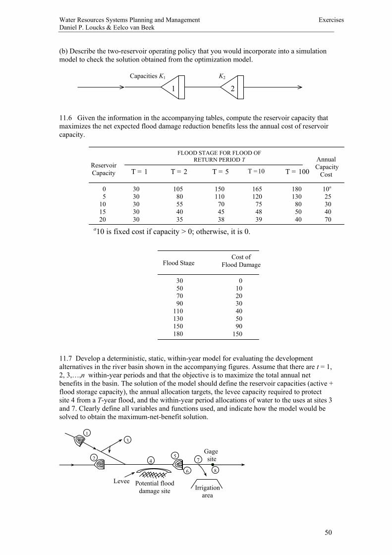
Water Resources Systems Planning and Management ExercisesDaniel P. Loucks & Eelco van Beek
50
(b) Describe the tworeservoir operating policy that you would incorporate into a simulationmodel to check the solution obtained from the optimization model.
11.6 Given the information in the accompanying tables, compute the reservoir capacity thatmaximizes the net expected flood damage reduction benefits less the annual cost of reservoircapacity.
11.7 Develop a deterministic, static, withinyear model for evaluating the developmentalternatives in the river basin shown in the accompanying figures. Assume that there are t = 1,2, 3,… ,n withinyear periods and that the objective is to maximize the total annual netbenefits in the basin. The solution of the model should define the reservoir capacities (active +flood storage capacity), the annual allocation targets, the levee capacity required to protectsite 4 from a Tyear flood, and the withinyear period allocations of water to the uses at sites 3and 7. Clearly define all variables and functions used, and indicate how the model would besolved to obtain the maximumnetbenefit solution.
ReservoirCapacity
FLOOD STAGE FOR FLOOD OFRETURN PERIOD T Annual
CapacityCost
05
101520
T = 1 T = 2 T = 5 T =10 T = 100
3030303030
10580554035
150110704538
165120754839
180130805040
10a
25304070
a10 is fixed cost if capacity > 0; otherwise, it is 0.
Flood StageCost of
Flood Damage
30507090
110130150180
0102030405090
150
Levee Potential flooddamage site Irrigation
area
Gage site
1
2
3
45
6
7
8
1 2
Capacities K1 K2

Water Resources Systems Planning and Management ExercisesDaniel P. Loucks & Eelco van Beek
51
For simplicity assume no evaporation losses or dead storage requirements. Omitting theappropriate subscripts t for time periods and s for site, let T, K, D, E, and P be the target,reservoir capacity, deficit, excess, and power plant capacity variables, respectively. Let Qtand Rt be the natural streamflows and reservoir releases, and St be the initial reservoir storagevolumes in period t. Kf will denote the flood storage capacity at site 2 that will contain a peakflow of QS and QR is the downstream channel flood flow capacity. The relationship betweenQS and Kf is defined by the function k(QS). The unregulated design flood peak flow forwhich protection is required is QN. KWH will be the kilowatt hours of energy, H will be netstorage head, ht the hours in a period t. The variable q will be the water supply allocation.Benefit functions will be B( ), L( ) will denote loss functions and C( ) will denote the costfunctions.
11.8 List the potential difficulties involved when attempting to structure models for defining:(a) Water allocation policies for irrigation during the growing season.(b) Energy production and capacity of hydroelectric plants.(c) Dead storage volume requirements in reservoirs.(d) Active storage volume requirements in reservoir.(e) Flood storage capacities in reservoirs.(f) Channel improvements for flood damage reduction.(g) Evaporation and seepage losses from reservoirs.(h) Water flow or storage targets using longrun benefits and short run loss
functions.
11.9 Assume that demand for water supply capacity is expected to grow as t(60 –t), for t inyears. Determine the minimum present value of construction cost of some subset of watersupply options described below so as to always have sufficient capacity to meet demandover the next 30 years. Assume that the water supply network currently has no excesscapacity so that some project must be built immediately. In this problem, assume projectcapacities are independent and thus can be summed. Use a discount factor equal to exp (0.07 t). Before you start, what is your best guess at the optimal solution?
SiteFraction ofGage Flow
12
3
4
5
67
8
0.0.3
0.15
0.6
0.9
1.0
Potential reservoir for water supply,Potential reservoir for water supply,flood controlDiversion to a use, 60% of allocationreturned to riverExisting development, possible floodprotection from leveePotential reservoir for water supply,recreationHydropower; plant factor = 0.30Potential diversion to an irrigationdistrictGage site

Water Resources Systems Planning and Management ExercisesDaniel P. Loucks & Eelco van Beek
52
11.10 (a) Construct a flow diagram for a simulation model designed to define a storageyieldfunction for a single reservoir given known inflows in each month t for n years. Indicate howyou would obtain a steadystate solution not influenced by an arbitrary initial storage volumein the reservoir at the beginning of the first period. Assume that evaporation rates (mm permonth) and the storage volume/surface area functions are known.
(b) Write a flow diagram for a simulation model to be used to estimate the probability thatany specific reservoir capacity, K, will satisfy a series of known release demands, rt,downstream given unknown future inflows, it. You need not discuss how to generate possiblefuture sequences of streamflows, only how to use them to solve this problem.
11.11 (a) Develop an optimization model for finding the costeffective combination of floodstorage capacity at an upstream reservoir and channel improvements at a downstreampotential damage site that will protect the downstream site from a prespecifieddesign flood of return period T. Define all variables and functions used in the model.
(b) How could this model be modified to consider a number of design floods T andthe benefits from protecting the potential damage site from those design floods? Let
TBF be the annual expected flood protection benefits at the damage site for a floodhaving return periods of T.
(c) How could this model be further modified to include water supply requirements oftA to be withdrawn from the reservoir in each month t? Assume known natural flowsstQ at each site s in the basin in each month t.
(d) How could the model be enlarged to include recreation benefits or losses at thereservoir site? Let Ts be the unknown storage volume target and
stD be the
difference between the storage volume stS and the target Ts if s
tS –Ts > 0, and stE be
the difference if Ts – stS > 0. Assume that the annual recreation benefits B(Ts) are a
function of the target storage volume Ts and the losses ( )D stL D and ( )E s
tL E areassociated with the deficit s
tD and excess stE storage volumes.
11.12 Given the hydrologic and economic data listed below, develop and solve a linearprogramming model for estimating the reservoir capacity K, the flood storage capacity Kf, andthe recreation storage volume target T that maximize the annual expected flood controlbenefits, Bf(Kf), plus the annual recreation benefits, B(T), less all losses )( t
D DL and )( tE EL
associated with deficits Dt or excesses Et in the periods of the recreation season, minus theannual cost C(K) of storage reservoir capacity K. Assume that the reservoir must also providea constant release or yield of Y = 30 in each period t. The flood season begins at the beginningof period 3 and lasts through period 6. The recreation season begins at the beginning of period4 and lasts though period 7.
Project Number
1234
ConstructionCost Capacity
100115190270
200250450700
Period tInflows to reservoir
1 2 3 4 5 6 7 8 950 30 20 80 60 20 40 10 70

Water Resources Systems Planning and Management ExercisesDaniel P. Loucks & Eelco van Beek
53
12 Kf if Kf £ 5Bf(Kf) = 60 + 8(Kf 5) if 5 £ Kf £ 15
140 + 4(Kf 15) if Kf ³ 15
45 + 10 K if 0 £ Kf £ 5C(K) = 95 + 6(K 5) if 5 £ Kf £ 20
185 + 10(K 20) if 20 £ Kf £ 40385 + 15(K 40) if Kf ³ 40
B(T) = 9T where T is a particular unknown value of reservoir storage
)( tD DL = 4Dt where Dt is T –St if T ³ St
)( tE EL = 2 Et where Et is St –T if St ³ T
11.13 The optimal operation of multiple reservoir systems for hydropower productionpresents a very nonlinear and often difficult problem.
Use dynamic programming to determine the operating policy that maximizes the total annualhydropower production of a tworeservoir system, one downstream of the other. The releasesR1t from the upstream reservoir plus the unregulated incremental flow (Q2t –Q1t) constitutethe inflow to the downstream dam. The flows Q1t into the upstream dam in each of the fourseasons along with the incremental flows (Q2t –Q1t) and constraints on reservoir releases aregiven in the accompanying two tables:
Qt = inflowRt = release
(excess)
St = initialstorage
Kf = flood
Y = 30
15
45
5 20 40
12
10
15
K
C(K)6Bf (Kf)
Kf
5 150
12
84
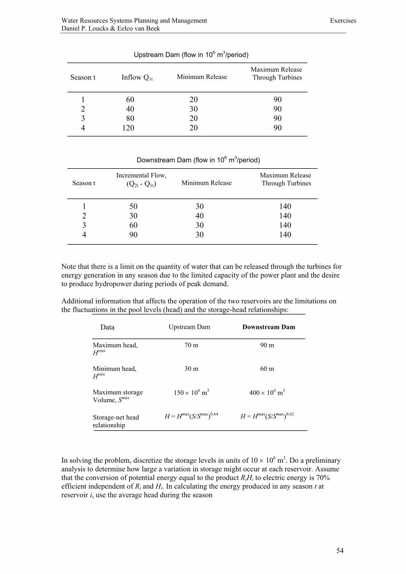
Water Resources Systems Planning and Management ExercisesDaniel P. Loucks & Eelco van Beek
54
Note that there is a limit on the quantity of water that can be released through the turbines forenergy generation in any season due to the limited capacity of the power plant and the desireto produce hydropower during periods of peak demand.
Additional information that affects the operation of the two reservoirs are the limitations onthe fluctuations in the pool levels (head) and the storagehead relationships:
In solving the problem, discretize the storage levels in units of 10 ´ 106 m3. Do a preliminaryanalysis to determine how large a variation in storage might occur at each reservoir. Assumethat the conversion of potential energy equal to the product RiHi to electric energy is 70%efficient independent of Ri and Hi. In calculating the energy produced in any season t atreservoir i, use the average head during the season
Season tMaximum Release Through Turbines
1234
Incremental Flow,(Q2t Q1t) Minimum Release
Downstream Dam (flow in 106 m3/period)
50306090
30403030
140140140140
Season tMaximum Release Through Turbines
1234
Inflow Q1t Minimum Release
Upstream Dam (flow in 106 m3/period)
604080
120
20302020
90909090
Data
Maximum head,Hmax
Minimum head,Hmin
Maximum storageVolume, Smax
Storagenet headrelationship
Upstream Dam
70 m
30 m
150 ´ 106 m3
H = Hmax(S/Smax)0.64
Downstream Dam
90 m
60 m
400 ´ 106 m3
H = Hmax(S/Smax)0.62
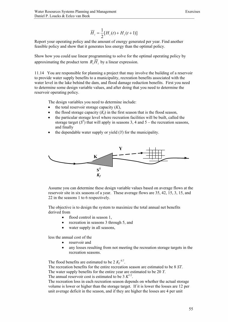
Water Resources Systems Planning and Management ExercisesDaniel P. Loucks & Eelco van Beek
55
)]1()([21
++= tHtHH iii
Report your operating policy and the amount of energy generated per year. Find anotherfeasible policy and show that it generates less energy than the optimal policy.
Show how you could use linear programming to solve for the optimal operating policy byapproximating the product term ii HR by a linear expression.
11.14 You are responsible for planning a project that may involve the building of a reservoirto provide water supply benefits to a municipality, recreation benefits associated with thewater level in the lake behind the dam, and flood damage reduction benefits. First you needto determine some design variable values, and after doing that you need to determine thereservoir operating policy.
The design variables you need to determine include:· the total reservoir storage capacity (K),· the flood storage capacity (Kf) in the first season that is the flood season,· the particular storage level where recreation facilities will be built, called the
storage target (ST) that will apply in seasons 3, 4 and 5 – the recreation seasons,and finally
· the dependable water supply or yield (Y) for the municipality.
Assume you can determine these design variable values based on average flows at thereservoir site in six seasons of a year. These average flows are 35, 42, 15, 3, 15, and22 in the seasons 1 to 6 respectively.
The objective is to design the system to maximize the total annual net benefitsderived from
· flood control in season 1,· recreation in seasons 3 through 5, and· water supply in all seasons,
less the annual cost of the· reservoir and· any losses resulting from not meeting the recreation storage targets in the
recreation seasons.
The flood benefits are estimated to be 2 Kf0.7.
The recreation benefits for the entire recreation season are estimated to be 8 ST.The water supply benefits for the entire year are estimated to be 20 Y.The annual reservoir cost is estimated to be 3 K1.2.The recreation loss in each recreation season depends on whether the actual storagevolume is lower or higher than the storage target. If it is lower the losses are 12 perunit average deficit in the season, and if they are higher the losses are 4 per unit
K
ST
Kf
Y

Water Resources Systems Planning and Management ExercisesDaniel P. Loucks & Eelco van Beek
56
average excess in the season. It is possible that a season could begin with a deficitand end with an excess, or vice versa.
Develop and solve a nonlinear optimization model for finding the values of each ofthe design variables: K, Kf, ST, and Y and the maximum annual net benefits. (Therewill be other variables as well. Just define what you need and put it all together in amodel.)
Does the solution give you sufficient information that would allow you to simulatethe system using a sequence of inflows to the reservoir that are different than the onesused to get the design variable values? If not how would you define a reservoiroperating policy? After determining the system’s design variable values usingoptimization, and then determining the reservoir operating policy, you would thensimulate this system over many years to get a better idea of how it might perform.
11.15 Suppose you have 19 years of monthly flow data at a site where a reservoir could belocated. How could you construct a model to estimate what the required overyear and withinyear storage needed to produce a specified annual yield Y that is allocated to each month t bysome known fraction dt. What would be the maximum reliability of those yields? If youwanted to add to that an additional secondary yield having only 80% reliability, how wouldthe model change? Make up 19 annual flows and assume the average monthly flows arespecified fractions of those annual flows. Just using these annual flows and the averagemonthly fractions, solve your model.
11.16 a) Develop an optimisation model for estimating the leastcost combination of activestorage K1 and K2 capacities at two reservoir sites on a single stream that are used to producea reliable flow or yield downstream of the downstream reservoir. Assume 10 years ofmonthly flow data at each reservoir site. Identify what other data are needed.
b) Describe the tworeservoir operating policy that could be incorporated into a simulationmodel to check the solution obtained from the optimization model
Define )( ss KC = cost of active storage capacity at site s; where s = 1, 2sdK = dead storage capacity of reservoir at site s; s
dK = 0stS = storage volume at beginning of period t at site s.sL = loss of water due to evaporation at site s; sL = 012tR = release from reservoir at site 1 to site 2 in period t
tY = yield to downstream in period tstQ = 10 years of monthly natural flows available at each site s
aos = area associated with dead storage volume at site s
as = area per unit storage volume at site set
s = evaporation depth in period t at site s
1 2
Capacities K1 K2

Water Resources Systems Planning and Management ExercisesDaniel P. Loucks & Eelco van Beek
57
11.16 Given inflows to an effluent storage lagoon that can be described by a simple firstorder Markov chain in each of T periods t, and an operating policy that defines the lagoondischarge as a function of the initial volume and inflow, indicate how you would estimate theprobability distribution of lagoon storage volumes.
11.17 (a) Using the inflow data in the table below, develop and solve a yield model forestimating the storage capacity of a single reservoir required to produce a yield of 1.5that is 90% reliable in both of the two withinyear periods t, and an additional yieldof 1.0 that is 70% reliable in period t = 2.(b) Construct a reservoiroperating rule that defines reservoir release zones for theseyields.(c ) Using the operating rule, simulate the 18 periods of inflow data to evaluate theadequacy of the reservoir capacity and storage zones for delivering the required yieldsand their reliabilities. (Note that in this simulation of the historical record the 90%reliable yield should be satisfied in all the 18 periods, and the incremental 70%reliable yield should fail only two times in the 9 years.)(d) Compare the estimated reservoir capacity with that which is needed using thesequent peak procedure.
Year Period Inflow1
2
3
4
5
6
7
8
9
121212121212121212
1.03.00.52.51.02.00.51.50.50.50.52.51.05.02.55.51.54.5
11.19 One possible modification of the yield model of would permit the solution algorithm todetermine the appropriate failure years associated with any desired reliability instead ofhaving to choose these years prior to model solution. This modification can provide anestimate of the extent of yield failure in each failure year and include the economicconsequences of failures in the objective function. It can also serve as a means of estimatingthe optimal reliability with respect to economic benefits and losses. Letting Fy be theunknown yield reduction in a possible failure year y, then in place of apyYp in the overyearcontinuity constraint, the term (Yp –Fy) can be used. What additional constraints are needed toensure (1) that the average shortage does not exceed (1 apy)Yp or (2) that at most there are ffailure years and none of the shortages exceed (1 apy)Yp.
11.20 In Indonesia there exists a wet season followed by a dry season each year. In one are ofIndonesia all farmers within an irrigation district plant and grow rice during the wet season.This crop brings the farmer the largest income per hectare; thus they would all prefer tocontinue growing rice during the dry season. However, there is insufficient water during the

Water Resources Systems Planning and Management ExercisesDaniel P. Loucks & Eelco van Beek
58
dry season for irrigating all 5000 hectares of available irrigable land for rice production.Assume an available irrigation water supply of 32 ´ 106 m3 at the beginning of each dryseason, and a minimum requirement of 7000 m3/ha for rice and 1800 m3/ha for the secondcrop.
(a) What proportion of the 5000 hectares should the irrigation district managerallocate for rice during the dry season each year, provided that all availablehectares must be given sufficient water for rice or the second crop?
(b) Suppose that crop production functions are available for the two crops, indicatingthe increase in yield per hectare per m3 of additional water, upto 10, 000 m3/ha forthe second crop. Develop a model in which the water allocation per hectare, aswell as the hectares allocated to each crop, is to be determined, assuming aspecified price or return per unit of yield of each crop. Under what conditionswould the solution of this model be the same as in part (a)?
11.21 Along the Nile River in Egypt, irrigation farming is practiced for the production ofcotton, maize, rice, sorghum, full and short berseem for animal production, wheat, barley,horsebeans, and winter and summer tomatoes. Cattle and buffalo are also produced, andtogether with the crops that require labor, water. Fertilizer, and land area (feddans). Farmtypes or management practices are fairly uniform, and hence in any analysis of irrigationpolicies in this region this distinction need not be made. Given the accompanying datadevelop a model for determining the tons of crops and numbers of animals to be grown thatwill maximize (a) net economic benefits based on Egyptian prices, and (b) net economicbenefits based on international prices. Identify all variables used in the model.
Known parameters:Ci = miscellaneous cost of land preparation per feddan
EiP = Egyptian price per 1000 tons of crop iI
iP = international price per 1000 tons of crop iv = value of meat and dairy production per animalg = annual labor cost per workerfP = cost of P fertilizer per tonfN = cost of N fertilizer per tonYi = yield of crop i, tons/feddan
= feddans serviced per animal= tons straw equivalent per ton of berseem carryover from winter to summer
rw = berseem requirements per animal in winterswh = straw yield from wheat, tons per feddansba = straw yield from barley, tons per feddanrs = straw requirements per animal in summer
Nim = N fertilizer required per feddan of crop iPim = P fertilizer required per feddan of crop i
lim = labor requirements per feddan in month m, mandayswim = water requirements per feddan in month m, 1000 m3
him = land requirements per month, fraction (1 = full month)
Required Constraints. (assume known resource limitations for labor, water, andland):(a) Summer and winter fodder (berseem) requirements for the animals.(b) Monthly labor limitations.(c) Monthly water limitations.(d) Land availability each month.(e) Minimum number of animals required for cultivation.

Water Resources Systems Planning and Management ExercisesDaniel P. Loucks & Eelco van Beek
59
(f) Upper bounds on summer and winter tomatoes (assume these are known).(g) Lower bounds on cotton areas (assume this is known).
Other possible constraints:(a) Crop balances.(b) Fertilizer balances.(c) Labor balance.(d) Land balance.
11.22 In Algeria there are two distinct cropping intensities, depending upon the availabilityof water. Consider a single crop that can be grown under intensive rotation or extensiverotation on a total of A hectares. Assume that the annual water requirements for the intensiverotation policy are 16000 m3 per hectare, and for the extensive rotation policy they 4000 m3
per hectare. The annual net production returns are 4000 and 2000 dinars, respectively. If thetotal water available is 320,000 m3, show that as the available land area A increases, therotation policy that maximizes total net income changes from one that is totally intensive toone that is increasingly extensive.
Would the same conclusion hold if instead of fixed net incomes of 4000 and 2000 dinars perhectares of intensive and extensive rotation, the net income depended on the quantity of cropproduced? Assuming that intensive rotation produces twice as much produced by extensiverotation, and that the net income per unit of crop Y is defined by the simple linear function 5 –0.05Y, develop and solve a linear programming model to determine the optimal rotationpolicies if A equals 20, 50, and 80. Need this net income or price function be linear to beincluded in a linear programming model?
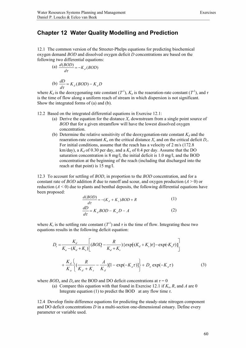
Water Resources Systems Planning and Management ExercisesDaniel P. Loucks & Eelco van Beek
60
Chapter 12 Water Quality Modelling and Prediction
12.1 The common version of the StreeterPhelps equations for predicting biochemicaloxygen demand BOD and dissolved oxygen deficit D concentrations are based on thefollowing two differential equations:
(a) )()( BODKdBODd
d-=t
(b) DKBODKddD
ad -= )(t
where Kd is the deoxygenating rate constant (T1), Ka is the reaerationrate constant (T1), andis the time of flow along a uniform reach of stream in which dispersion is not significant.Show the integrated forms of (a) and (b).
12.2 Based on the integrated differential equations in Exercise 12.1:(a) Derive the equation for the distance Xc downstream from a single point source of
BOD that for a given streamflow will have the lowest dissolved oxygenconcentration.
(b) Determine the relative sensitivity of the deoxygenationrate constant Kd and thereaerationrate constant Ka on the critical distance Xc and on the critical deficit Dc.For initial conditions, assume that the reach has a velocity of 2 m/s (172.8km/day), a Kd of 0.30 per day, and a Ka of 0.4 per day. Assume that the DOsaturation concentration is 8 mg/l, the initial deficit is 1.0 mg/l, and the BODconcentration at the beginning of the reach (including that discharged into thereach at that point) is 15 mg/l.
12.3 To account for settling of BOD, in proportion to the BOD concentration, and for aconstant rate of BOD addition R due to runoff and scour, and oxygen production (A > 0) orreduction (A < 0) due to plants and benthal deposits, the following differential equations havebeen proposed:
RBODKKdBODd
sd ++-= )()(t
(1)
ADKBODKddD
ad --=t
(2)
where Ks is the settling rate constant (T1) and is the time of flow. Integrating these twoequations results in the following deficit equation:
úû
ùêë
é--+-
+-
+-= )}exp(])(){exp[(
)(ttt asd
sdo
sda
d KKKKK
RBODKKK
KD
)exp()]exp(1)[( tt aoadsda
d KDKKA
KKR
KK
-+þýü
îíì
---+
+ (3)
where BODo and Do are the BOD and DO deficit concentrations at = 0(a) Compare this equation with that found in Exercise 12.1 if Ks, R, and A are 0
Integrate equation (1) to predict the BOD at any flow time .
12.4 Develop finite difference equations for predicting the steadystate nitrogen componentand DO deficit concentrations D in a multisection onedimensional estuary. Define everyparameter or variable used.

Water Resources Systems Planning and Management ExercisesDaniel P. Loucks & Eelco van Beek
61
12.5 Using MichaelisMenten kinetics develop equations for
(a) Predicting the time rate of change of a nutrient concentration N (dN/dt) as afunction of the concentration of bacterial biomass B;
(b) Predicting the time rate of change in the bacterial biomass B(dB/dt) as a functionof its maximum growth rate max
Bm , temperature T, B, N, and the specificloss rateof bacteria rB; and
(c) Predicting the time rate of change in dissolved oxygen deficit (dD/dt) also as afunction of N, B, rB, and the reaerationrate constant Ka (T1).
How would these three equations be altered by the inclusion of protozoa P that feed onbacteria, and in turn require oxygen? Also write the differential equations for the time rate ofchange in the concentration of protozoa P(dP/dt).
12.6 Most equations for predicting stream temperature are expressed in Eulerian coordinates.The actual behavior of the stream temperature is more easily demonstrated if Lagrangiancoordinates (i.e., time of flow t rather than distance X) are used. Assuming insignificantdispersion, the “timeofflow” rate of temperature change of a water parcel as it moves downstream is
)( TTcDd
dTE -=
rl
t
(a) Assuming that l, D, and TE are constant over interval of time of flow t2 –t1,integrate the equation above to derive the temperature T1 at locations X1.
(b) Develop a model for predicting the temperature at a point in a nondispersivestream downstream from multiple point sources (discharges) of heat.
12.7 Consider three wellmixed bodies of water that have the following constant volumesand freshwater inflows:
The first body is representative of the Great Lakes in North America, the second ischaracteristic in size to the upper New York harbor with the summer flow of the HudsonRiver, and the third is typical of a small bay or cove. Compute the time required to achieve99% of the equilibrium concentration, and that concentration, of a substance having an initialconcentration, and that concentration, of a substance having an initial concentration of 0 (attime = 0) and an input of N (MT1) for each of the three water bodies. Assume that the decayrate constant K is 0, 0.01, 0.05, 0.25, 1.0, and 5.0 days1 and compare the results.
12.8 Consider the water pollution problem as shown in the Figure below. There are twosources of nitrogen, 200 mg/l at site 1 and 100 mg/l at site 2, going into the river, whereas thenitrogen concentration in the river just upstream of site 1 is 32 mg/l. The unknown variablesare the fraction of nitrogen removal at each of those sites that would achieve concentrationsno greater than 20 mg/l and 25 mg/l just upstream of site 2 and at site 3 respectively, at a totalminimum cost. Let those nitrogen removal fractions be X1 and X2.
Water Body Volume (m3)
123
3 ´ 1012
3 ´ 108
3 ´ 104
Flow (m3/s)Displacement
Time
3 ´ 103
3 ´ 102
3
3.17 years11.6 days2.8 hours

Water Resources Systems Planning and Management ExercisesDaniel P. Loucks & Eelco van Beek
62
Assuming unit costs of removal as $30 and $20 at site 1 and site 2 respectively, the model canbe written as:
Minimize 30 X1 + 20 X2
Subject to: 200(1 X1)0.25 + 8 £ 20200(1 X1)0.15 + 100(1 –X2)0.60 + 5 £ 25X1 £ 0.9, X2 £ 0.9
Another way to write the two quality constraints of this model is to define variables Si(i=1,2,3) as the concentration of nitrogen just upstream of site i. Beginning with aconcentration of 32 mg/l just upstream of site 1, the concentration of nitrogen just upstream ofsite 2 will be
[32 + 200(1 X1)]0.25 = S2 and S2 £ 20.
The concentration of nitrogen at site 3 will be
[S2 + 100(1 X2)]0.60 = S3 and S3 £ 25.
This makes the problem easier to solve using discrete dynamic programming. The nodes orstates of the network can be discrete values of Si, the concentration of nitrogen in the river atsites i (just upstream of sites 1 and 2 and at site 3). The links represent the decision variablevalues, Xi that will result in the next discrete concentration, Si+1 given Si. The stages i are thedifferent source sites or river reaches. A section of the network in stage 1 (reach from site 1 tosite 2) will look like:
So if S2 is 20, X1 will be 0.76; if S2 is 15, X1 will be 0.86. For S2 values of 10 or less X1 mustexceed 0.90 and these values are infeasible. The cost associated with the link or decision willbe 30 X1.
Setup the dynamic programming network. It begins with a single node representing the state(concentration) of 32 mg/l just upstream of site 1. It will end with a single node representingthe state (concentration) 25 mg/l. The maximum possible state (concentration value justupstream of site 2 must be no greater than 20 mg/l. You can use discrete concentration valuesin increments of 5 mg/l. This will be a very simple network. Find the leastcost solution usingboth forward and backward moving dynamic programming procedures. Please show yourwork.
12.9 Identify a three alternative sets (feasible solutions) of storage lagoon volume capacitiesV and corresponding land application areas A and irrigation volumes Q2t in each month t within a year that satisfy a 10 mg/l maximum NO3N content in the drainage water of a landdisposal system. In addition to the data listed below, assume that the influent nitrogen n1t is 50mg/l each month, with 10% ( = 0.1) of the nitrogen in organic form. Also assume that thesoil is a welldrained silt loam containing 4500 kg/ha of organic nitrogen in the soil above thedrains. The soil has a monthly drainage capacity d of 60 cm and has a field capacity moisture
200 mg/l
100 mg/l
32 mg/l
32 S2[32 + 200(1 X1)]0.25 = S2
12 3

Water Resources Systems Planning and Management ExercisesDaniel P. Loucks & Eelco van Beek
63
content M of 10 cm. Maximum plant nitrogen uptake values Ntmax are 35 kg/ha during April
through October, and 70 kg/ha during May through September. Finally, assume that becauseof cold temperatures, no wastewater irrigation is permitted during November through March.December, January, and February’s precipitation is in the form of snow and will melt and beadded to the soil moisture inventory in March.
12.10 Consider the problem of estimating the minimum total cost of waste treatment in orderto satisfy quality standards within a stream. Let the stream contain seven homogenous reachesr, reach r = 1 being at the upstream end and reach r = 7 at the downstream end. Reaches r = 2and 4 are tributaries entering the mainstream at the beginning of 1, 3, 5, 6, and 7. Pointsources of BOD enter the stream at the beginning of reaches 1, 2, 3, 4, 6, and 7. Assumingthat at least 60% BOD removal is required at each discharge site, solve for the leastcostsolution given the data in the accompanying table. Can you identify more than one type ofmodel to solve this problem? How would this model be expanded to specifically include bothcarbonaceous BOD and nitrogenous BOD and nonpoint waste discharges?
12.11 Discuss what would be required to analyze flow augmentation alternatives in Exercise12.8 How would the costs of flow augmentation be defined and how would you modify themodel(s) developed in Exercise 12.8 to include flow augmentation alternatives?
12.12 Develop a dynamic programming model to estimate the leastcost number, capacity,and location of artificial aerators to ensure meeting minimum allowable dissolved oxygenstandards where they would otherwise be violated during an extreme lowflow designcondition in a nonbranching section of a stream. Show how wastewater treatment alternatives,and their costs, could also be included in the dynamic programming model.
12.13 Using the data provided, find the steadystate concentrations Ct of a constituent in awellmixed lake of constant volume 30 ´ 106 m3. The production Nti of the constituent occursat three sites i, and is constant in each of four seasons in the year. The required fractions ofconstituent removal Pi at each site i are to be set so that they are equal at all sites i and themaximum concentration in the lake in each period t must not exceed 20 mg/l.
ReachNo.
DesignBODLoad
(mg/l)
Present% Removal
Load
ANNUAL COSTSOF VARIOUS DESIGN BOD REMOVALS
60% 75% 85% 90%123467
24840824014402180279
673030303030
0630,000210,000413,000500,000840,000
22,100780,000277,500523,000638,000
1,072,000
77,500987,000323,000626,000790,000
1,232,500
120,6001,170,000
378,000698,000900,000
1,350,000
ReachNo.
Time ofFlow(days)
WasteWater
Discharge(103m3/day)
1234567
EnteringReachFlow
(103m3/day)
TotalReachFlow
(103m3/day)
DOsaturation
conc.(mg/l)
MaximumallowableDO Deficit
(mg/l)
DODeficit
of wastewater(mg/l)
DO Concat begi
nning ofReach(mg/l)
Av. Deoxgnrate
constant forReach
(days1)
ReaerationRate
constant(days1)
0.2351.3301.0872.0670.3061.0506.130
1914030530
98155
5,1294,883
10,1711,120
11,37411,37411,472
5,1485,023
10,2011,173
11,37411,47211,627
10.209.959.009.709.008.358.17
3.202.452.003.752.502.354.17
1.01.01.01.0
1.01.0
9.508.00
?9.54
?
BOD Concat begi
nning ofReach(mg/l)
1.660.68
?1.0?
0.310.410.360.350.340.350.30
1.020.600.630.090.720.140.02
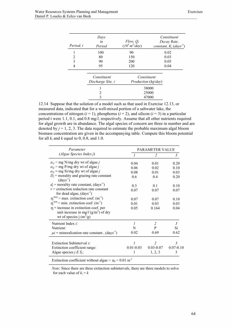
Water Resources Systems Planning and Management ExercisesDaniel P. Loucks & Eelco van Beek
64
12.14 Suppose that the solution of a model such as that used in Exercise 12.13, ormeasured data, indicated that for a wellmixed portion of a saltwater lake, theconcentrations of nitrogen (i = 1), phosphorus (i = 2), and silicon (i = 3) in a particularperiod t were 1.1, 0.1, and 0.8 mg/l, respectively. Assume that all other nutrients requiredfor algal growth are in abundance. The algal species of concern are three in number and aredenoted by j = 1, 2, 3. The data required to estimate the probable maximum algal bloombiomass concentration are given in the accompanying table. Compute this bloom potentialfor all ki and k equal to 0, 0.8, and 1.0.
Parameter(Algae Species Index j)
PARAMETER VALUE1 2 3
a1j = mg N/mg dry wt of algae ja2j = mg P/mg dry wt of algae ja3j = mg Si/mg dry wt of algae jDj = morality and grazing rate constant (days1)dj = morality rate constant, (days1)v = extinction reduction rate constant for dead algae, (days1)hj
max = max. extinction coef. (m1)hj
min = min. extinction coef. (m1)hj = increase in extinction coef. per unit increase in mg/l (g/m3) of dry wt of species j (m2/g)
0.040.060.080.6
0.30.07
0.070.010.05
0.010.020.010.4
0.10.07
0.070.030.164
0.200.100.030.20
0.100.07
0.100.030.04
Nutrient Index i:Nutrient:mi = mineralization rate constant , (days1)
1N
0.02
2P
0.69
3Si
0.62
Extinction Subinterval s:Extinction coefficient range:Algae species j E Ss:
10.010.03
1
20.030.07
1, 2, 3
30.070.10
3
Extinction coefficient without algae = h0 = 0.01 m1
Note: Since there are three extinction subintervals, there are three models to solvefor each value of ki = k
Period, t
Daysin
PeriodFlow, Qt
(103 m3/day)
1234
ConstituentDecay Rate,
constant, Kt (days1)100809095
90150200120
0.020.030.050.04
123
ConstituentDischarge Site, i
380002500047000
ConstituentProduction (kg/day)
Water Resources Systems Planning and Management ExercisesDaniel P. Loucks & Eelco van Beek
65
Chapter 13 Urban Water Systems
13.1 Define the components of the infrastructure needed to bring water into your home andthen collect the wastewater and treat it prior to discharging it back into a receiving waterbody. Draw a schematic of such a system and show how it can be modeled to determine thebest design variable values. Define the data needed to model such a system and then make upvalues of the needed parameters and solve the model of the system.
13.2 Compare the curve number approach to the use of Manning’s equation to estimateurban runoff quantities. Then define how you would predict quality and sediment runoff aswell.
13.3 Develop a simple model for predicting the runoff of water, sediment and severalchemicals from a 10ha urban watershed in the northeastern United States during August1976. Recorded precipitation was as follows:
Solids (sediment) buildup on the watershed at the rate of 50 kg/haday, and chemicalconcentrations in the solids are 100 mg/kg. Assume that each runoff event washes thewatershed surface clean. Assume also that there is no initial sediment buildup on August. Thewatershed is 30% impervious. For each storm use your model to compute:
(a) Runoff in cm and m3.(b) Sediment loss (kg).(c) Chemical loss (g), in dissolved and solidphase form for chemicals with three
different adsorption coefficients, k = 5, 100, 1000.
13.4 There exists a modestsized urban subdivision of 100 ha containing 2000 people. Landuses are 60% singlefamily residential, 10% commercial, and 30% undeveloped. Anevaluation of the effects of street cleaning practices on nutrient losses in runoff is required forthis catchment.
This evaluation is to be based on the 7month precipitation record given below. Present theresults of the simulations as 7month PO4 and N losses as functions of streetcleaning intervaland efficiency (i.e., show these losses for ranges of intervals and efficiencies). Assume arunoff threshold for washoff of Qo = 0.5 cm.
Day 1 6 7 8 9 10 13 14 15 26 29
Rt (cm) 1.8 0.7 2.6 2.9 0.1 0.3 2.9 0.1 1.4 3.7 0.8
Water Resources Systems Planning and Management ExercisesDaniel P. Loucks & Eelco van Beek
66
Day A12345678910111213141516171819202122232425262728293031
PRECIPITATION (cm)M J J A S O
1.1
0.10.10.1
0.1
0.1
0.12.03.20.1
0.4
1.50.9
0.10.6
0.5
0.1
0.20.1
0.6
1.40.1
1.6
0.2
0.70.40.40.7
0.6
0.31.1
1.41.10.70.1
0.20.2
0.80.1
0.3
0.1
3.0
0.3
1.4
1.91.00.7
0.1
0.2
0.5
0.5
0.4
0.2
0.60.2
0.70.50.1
0.3
1.53.5
4.30.80.80.42.30.3
4.72.81.6
0.1
1.9
0.1
0.5
0.41.5
0.2
0.81.02.81.90.10.9
Water Resources Systems Planning and Management ExercisesDaniel P. Loucks & Eelco van Beek
67
Chapter 14 A Synopsis
14.1 Identify, research, describe and critique a water resources planning and managementcase study. Describe the system being studied, how it was studied or modeled, theinstitutional setting, the objectives to be accomplished, and your evaluation of how the studywas carried out. Was a systems approach applied to the particular water resourcesmanagement problem. Evaluate the effectiveness of any modeling, the extent of stakeholderparticipation, and how, if applicable, with hindsight the study could have been improved.
14.2 The following factors are among those that are impacting our global as well as localwater systems. Briefly identify their causes and resulting global impacts.
a) Climate changeb) Basin scale water balance changesc) River flow regulationd) Sediment fluxese) Chemical pollutionf) Microbial pollutiong) Biodiversity changes
14.3 Presented below are some conclusions of a recent conference on water and sustainability(Schiffries and Brewster, editors, 2004, Water for a Sustainable and Secure Future, NationalCouncil for Science and the Environment, Washington, DC). Write a brief critical discussionof each of these statements.
a) Water is an essential part of human welfare — maintaining our health andsurvival, protecting sensitive ecosystems, producing an ample food supply, promoting overalleconomic prosperity, enhancing recreation and aesthetics, and providing for the longtermsecurity of individuals and nations.
b) Providing enough water for human needs is challenging water policymakers,especially in the water scarce regions, largely because water has been viewed as a freecommodity. For this reason, it is typically delivered at vastly below cost and usedinefficiently.
c) The United States had the worst water efficiency of 147 countries ranked by theWorld Water Council, a status that is linked to low water prices. The (2004) price of water inthe United States averages $0.54 per cubic meter, compared to $1.23 for the United Kingdomand $1.78 for Germany.
d) Perhaps the most important management issue regarding water and sanitation, theone that could have the most benefit for the poor is progressive pricing — ”charging more perunit the more water is used” — to ensure that people can afford enough water to livehealthfully and still provide incentives for efficient use.
e) The world is in “a water crisis” that is getting worse. Population is growing mostrapidly where water is least available, and water will be among the first resources affected byrising global temperatures and the resulting climate change. This water crisis can be alleviatedby pursuing solutions that involve communityscale water systems, open and decentralizeddecisionmaking, and greater efficiency.
f) Profound misunderstanding of water science has been institutionalized in manystates, where groundwater and surface water are legally two unrelated entities. This gap has
Water Resources Systems Planning and Management ExercisesDaniel P. Loucks & Eelco van Beek
68
led to practices of unsustainable groundwater withdrawal in some areas and ineffective watermanagement policies that do not take a holistic approach. Ground water and surface water areinextricably linked through the hydrologic cycle, and we need to reform the governance ofsurface and ground water to reflect actual hydrologic linkages.
g) The challenge of 21st century river management is to better balance human waterneeds with the water needs of rivers themselves. Meeting this challenge may require afundamentally new approach to valuing and managing rivers. each component of a river’sflow pattern — the highs, the lows, and the levels in between — is important to the health ofthe river system and the life within it. He is optimistic that new policies will be based on agrowing scientific consensus that restoring some degree of a river’s natural flow pattern is thebest way to protect and restore river health and functioning.
h) Hydrological and ecological linkages, rather than political boundaries, shouldform the basis for water management. Governance structures should be designed to facilitate awatershed, basin or ecosystem approach to water management. For example, researchers areincreasingly attributing coastal pollution problems, such as nutrient overenrichment, deadzones, and toxic contamination, to diffuse sources far inland from coastal environments.Therefore, effective solutions to these issues must be holistic, entering at the watershed leveland connecting coastal pollution with inland sources.
14.4 How would you prioritize and implement the following water sustainabilityrecommendations contained in the report cited in exercise 14.3?
1. Develop a Robust Set of Indicators for Sustainable Water Management.2. Improve Data and Monitoring Systems for Sustainable Water Management.3. Advance Interdisciplinary Scientific Research on Sustainable Water Management.4. Integrate Social and Natural Science Research on Sustainable Water Management.5. Close the Gap Between Water Science and Water Policy.6. Develop a Spectrum of Technologies to Advance Sustainable Water Management.7. Improve Education and Outreach on Sustainable Water Management.8. Promote International Capacity Building on Sustainable Water Management.9. Establish National Commissions on Water Sustainability.


![ESA 2008/2009 Eelco Schatborn [email protected]](https://static.fdocuments.in/doc/165x107/623cf670266aa32a040f8f87/esa-20082009-eelco-schatborn-emailprotected.jpg)