Water wave scattering from a mass loading ice floe ofrandom length using generalised polynomial chaos

J. E. M. Mosiga,∗, F. Montiela, V. A. Squirea

aDepartment of Mathematics and Statistics, University of Otago, Dunedin, New Zealand

Abstract

We consider the scattering of water waves in a two dimensional domain from a

floating sea ice floe of random length. The length is treated as a random vari-

able governed by a prescribed probability distribution. To keep the focus on the

random length aspect we choose a simple mass loading model to characterise the

ice floe. We compute the expectation and variance of the reflection and trans-

mission coefficients using two different methods derived from the framework of

generalised polynomial chaos (gPC), as part of which unknown quantities of

the problem are expanded in a basis of orthogonal polynomials of the random

variable. The polynomials are chosen optimally for the particular probability

distribution of the random variable to minimise an approximation error. We

devise a stochastic collocation method, which involves computing the reflection

and transmission coefficients deterministically for a number of carefully sam-

pled lengths and fitting polynomial expansions to them. The second approach

is based on the stochastic Galerkin method, for which the governing equations

are transformed to accommodate the random length parameter. We also use a

standard Monte Carlo (MC) approach for comparison. The gPC methods are

shown to be numerically efficient and exhibit desirable exponential convergence

properties, as opposed to the slow inverse square root convergence of the MC ap-

proach. Finally, we use the statistic collocation method to demonstrate that the

∗Corresponding authorEmail addresses: jmosig@maths.otago.ac.nz (J. E. M. Mosig),

fmontiel@maths.otago.ac.nz (F. Montiel), vernon.squire@otago.ac.nz (V. A. Squire)

Preprint submitted to Wave Motion September 7, 2016

floe size distribution can have a significant impact on the expected transmission

coefficient.

Keywords: water wave scattering, random length, generalised polynomial

chaos

2

1. Introduction

The scattering of surface gravity waves from compliant floating structures is

a well studied problem in ocean engineering and polar geophysics (see e.g. [1]).

Floating structures include various man-made objects, such as very large floating

structures (VLFSs; see [2]), but also naturally occurring ones, such as sea ice5

floes [3]. The vast literature on wave scattering by such floating structures has

concentrated on characterising (i) the response of the structure to water wave

forcing and (ii) the scattered wave field generated from diffraction and radiation

processes. The geometry of the structure is typically known or is a function of a

number of deterministic parameters, so the method used to solve the scattering10

problem can be adapted to a certain class of geometries.

Various geometries have been considered in both two and three dimensions.

Meylan and Squire [4] devised a Green’s function method for the scattering of

ocean waves by a floating elastic beam with uniform thickness as a model for a

sea ice floe. The same problem was revisited in different fields and solved with15

a range of numerical methods, such as mode matching [5], integro-differential

equations [6] and an integral equation / Galerkin technique [7]. The extension

to non-uniform floating beams was considered in [8, 9, 10]. In three dimensions

the scattering of water waves by circular elastic plates of uniform thickness was

investigated by several authors [11, 12, 13]. Scattering by circular floes with20

axisymmetric thickness variations was later solved by Bennetts et al. [14] using

a multi-mode approximation. Finally, Meylan [15] and Bennetts and Williams

[16] developed methods for scattering by elastic plates of arbitrary shape with

constant thickness.

It is less clear, however, how uncertainties in the structure’s geometry affect25

the response of the structure and the scattered wave field. This is particularly

relevant in the case of sea ice floes, where the general shape varies significantly

between individual floes, depending on how they form and then interact with

their environment. Taking accurate in situ measurements of the shape and size

of individual floes is also challenging [17], so that these properties are usually30

3

given as empirical statistical distributions. To the best of our knowledge no

previous studies have attempted to quantify the uncertainty of the scattered

wave field due to random variations in the geometry of the structure.

In the present article we conduct a preliminary study to describe the scat-

tering of water waves in two dimensions (one horizontal and one vertical) from35

an ice floe of random length and uniform thickness. The probability distribu-

tion of the length variable is prescribed. We then seek to compute the central

moments, i.e. expectation and variance, of the probability distributions of the

transmission and reflection coefficients of the ice floe.

Many different methods are available to handle uncertainties in geometry.40

These include perturbation methods, moment equations, and the Monte Carlo

(MC) approach [18]. Perturbation methods, however, typically require pertur-

bations of the parameters and the response of the system to remain small, while

the MC approach is known to exhibit slow convergence properties. Here we

employ the framework of generalised polynomial chaos (gPC), which does not45

constrain the size of the random perturbation and converges fast when the sys-

tem’s dependence on the random variables is sufficiently smooth and the number

of random variables is small [19].

For problems involving multiple random variables, gPC methods can be

problematic as the size of the system of equations arising in such problems50

increases with the factorial of the random dimension. For example Ganesh

and Hawkins [20] found that gPC methods are only practical when the num-

ber of random variables is less than 5, but the technique can be extended to

a sparse-grid gPC method, which works for more random variables at the ex-

pense of reduced accuracy. We also note that, for more complicated problems,55

such as non-linear wave–body interaction, the quantities of interest may not

depend smoothly on the random variable(s), in which case gPC methods would

exhibit poor convergence properties. Computationally more intense remedies

exist, however, e.g., multi-element gPC methods [21] or wavelet gPC basis func-

tions [22].60

The problem considered here involves smooth functions and only a single

4

random variable (the length of the floe). Consequently, gPC techniques are ide-

ally suited and fast numerical convergence can be expected. The key idea of gPC

techniques is to expand the random variable in a basis of mutually orthogonal

polynomials. The choice of the polynomial basis is informed by the probability65

distribution of the random variable. The polynomial expansion provides a spec-

tral representation of the variable in random space, so the scattering problem

can be solved using conventional spectral techniques, e.g. mode matching or

integral equations.

As the focus of the present work is to introduce the use of gPC methods in70

a water wave scattering problem, we consider the canonical mass loading model

to describe the vertical motion of the ice floe, which does not account for the

elasticity of the structure. We acknowledge that the mass loading model is too

simple to characterise the motion of an ice floe properly, noting that it has been

used by Keller and Weitz [23] to represent pack ice, and later by Wadhams75

and Holt [24] to represent floating frazil ice. The more standard thin elastic or

visco-elastic plate models could be used instead, but this would introduce un-

necessary complexity in the implementation of the gPC framework and would

not affect the results aimed at demonstrating the efficiency of the framework in

a one-dimensional wave scattering problem. The present article also provides80

the foundation for the extension to three dimensional models where the notion

of random length evolves into the notion of random shape. The random bound-

ary of a three dimensional ice floe may then, for example, be described by a

Karhunen-Loeve expansion in a small number of random variables. Although

new issues arise in the three dimensional setting, such as multiple random vari-85

ables, the basic ideas should carry over in a straightforward manner.

We begin our analysis in §2 with a detailed description of the random floe

problem. After briefly discussing the well known fixed length problem in §3,

we solve the random length problem using two different gPC methods in §4.

Numerical results for both methods are presented in §5 and compared to the90

MC approach. The focus of the Results section is to demonstrate the attractive

convergence properties of the gPC framework for the problem considered here.

5

As an example, we utilize the good performance of the gPC method to investi-

gate the length-distribution dependence of the expected reflection coefficient of

a mass loading floe as a function of floe thickness and wave period. Finally, we95

conclude with a discussion of our findings in §6.

6

0

-H

0 L

h

x

z

Figure 1: Geometry of the problem.

2. Preliminaries

We consider a two dimensional (one horizontal and one vertical) water do-

main which is infinitely long horizontally and has finite extent in the vertical

direction. In a Cartesian coordinate system (x, z), the vertical dimension is100

bounded by the equilibrium water surface at z = 0 and the flat sea floor at z =

−H. The water domain is denoted by Ω = (x, z),−∞ < x <∞,−H < z < 0.

A sea ice floe of thickness h covers the equilibrium water surface between x = 0

and x = L. For simplicity, we assume the draught of the floe can be neglected.

A sketch of the geometry is shown in figure 1.105

The water is modelled as an incompressible and inviscid fluid of density ρ =

1025 kg m−3. Further, assuming irrotational and time-harmonic motion, the ve-

locity field of the fluid particles can be expressed as Re(∂x, ∂z)φ(x, z) exp(−iω t),

where ω is the angular frequency and t denotes time. The fluid motion is then

fully described by the complex velocity potential φ(x, z). The time-harmonic110

condition allows us to replace ∂t = −iω throughout. The incompressibility

assumption applied together with mass conservation implies that φ satisfies

Laplace’s equation

(∂2x + ∂2z )φ = 0 , for (x, z) ∈ Ω . (1)

In addition, linearity and conservation of momentum implies that φ satisfies the

7

linearised form of Bernoulli’s equation115

iω ρφ = ρ g z − p , for (x, z) ∈ Ω , (2)

where g = 9.8 m s−2 is the acceleration due to gravity, and p is the water pres-

sure.

The vertical motion of the ice floe is described by the mass loading model,

which corresponds to the Euler-Bernoulli beam equation in the limit of vanishing

elasticity. The pressure load p on the beam is then given by120

p = ω2 ρ h η , (3)

where η = η(x) is the surface elevation, h is the thickness of the floe and

ρ = 917 kg m−3 is the density of sea ice. Note that the fourth order derivative

that appears in the Euler-Bernoulli beam equation [25] is absent in (3). At

z = 0 the kinematic surface condition holds, i.e.

−iω η = ∂zφ , z = 0 . (4)

The free surface condition125

g ∂zφ = ω2 φ , z = 0, x < 0, x > L , (5)

follows from (2) and (4). Similarly, assuming p = −p on the bottom surface of

the floe and using (2), (4) and (3) yields the mass loading surface condition

(g − ω2 ρ h

)∂zφ = ω2 φ , z = 0, x ≥ 0 . (6)

At the rigid sea floor, the vertical fluid velocity should vanish, i.e.

∂zφ = 0 , z = −H . (7)

We prescribe a wave forcing with velocity potential

φIn(x, z) = A0 eiκ0 x ς0(z) , (8)

characterising a plane wave travelling in the positive x-direction. The wavenum-130

ber κ0 and vertical function ς0(z) will be defined in §3. The presence of the ice

8

floe gives rise to reflected and transmitted wave components, which are given

by

φ(x, z)→ φIn(x, z) +RA0 e−iκ0 x ς0(z) , as x→ −∞ (9)

and

φ(x, z)→ T A0 eiκ0 x ς0(z) , as x→∞ , (10)

respectively, where R and T denote the unknown reflection and transmission135

coefficients.

9

A-

B-

A+

B+

SL

V-

W-

V+

W+

S0

C-

D-

C+

D+

SR

Figure 2: Separation of the deterministic scattering problem into three sub-problems, i.e. scat-

tering from the left edge, phase change of the wave under the floe, and scattering from the

right edge.

3. Fixed length scattering

Let us first assume that the length of the ice floe L is a given constant.

The scattering problem can be separated into three sub-problems, namely (i)

scattering from the left edge, (ii) wave propagation under the floe, and (iii)140

scattering from the right edge (see figure 2). The solutions of these sub-problems

are then combined to describe the scattering by the fixed length ice floe.

3.1. Scattering from the floe edges

We first consider the scattering of waves by the floe’s left edge located at x =

0. On either side of the edge, we separate variables and represent the solution to145

Laplace’s equation (1) by a plane wave ansatz. Imposing the sea floor condition

(7), the free surface condition (5) for x < 0 and the mass loading condition (6)

for x ≥ 0, we approximate the potential as truncated series expansions of Nζ+1

plane wave modes, i.e.

φ(x, z) ≈ φ−(x, z) =

Nζ∑n=0

(A−n e

iκn x +B−n e

−iκn x)ςn(z) , x ≤ 0 , (11)

on the left (open water) side of the edge and150

φ(x, z) ≈ φ+(x, z) =

Nζ∑n=0

(A+n e

i kn x +B+n e

−i kn x)ζn(z) , x ≥ 0 , (12)

on its right (ice-covered) side. We have introduced the vertical modes in the

open water and ice-covered domains given by

ςn(z) =cosh (κn (H + z))

cosh (κnH), (13)

10

and

ζn(z) =cosh (kn (H + z))

cosh (knH), (14)

respectively. The wavenumbers κn and kn satisfy their respective dispersion

relations, i.e.155

κ tanh(κH)− ω2

g= 0 , (15)

in the open water domain, and

k tanh(kH)− ω2

g − hω2/ρ= 0 , (16)

in the ice-covered domain. Both dispersion relations have one real and infinitely

many imaginary solutions in the first quadrant of the complex plane. The re-

maining solutions are the negatives of these and are included in the expansions

(11) and (12). The real solutions of (15) and (16) are denoted by κ0 and k0,160

respectively. These solutions are associated with propagating wave modes which

do not attenuate with x. We sort the imaginary solutions by increasing magni-

tude of their imaginary part, i.e. Imkn+1 > Imkn and Imκn+1 > Imκn,

for n ≥ 1. These correspond to evanescent modes decaying exponentially faster

with x as n increases. The truncation of the sums in (11) and (12) at finite Nζ165

is therefore justified.

Let the vectors A− = (A−0 , . . . , A

−Nζ

)T and B− = (B−0 , . . . , B

−Nζ

)T, respec-

tively, contain the complex amplitudes of the right and left propagating modes

in the general solution (11). Furthermore, let the vectors A+ = (A+0 , . . . , A

+Nζ

)T

and B+ = (A+0 , . . . , A

+Nζ

)T, respectively, contain the amplitudes of the right170

and left propagating modes in the general solution (12). By matching the po-

tentials φ− = φ+ and horizontal fluid velocities ∂xφ− = ∂xφ

+ at the boundary

x = 0, we can find the following set of relationships describing the reflection

and transmission of waves incident on either side of the edge

A+ = T−L ·A

− +R+L ·B

+ , (17)

B− = R−L ·A

− + T+L ·B

+ . (18)

where T±L and R±

L are matrices of dimension (Nζ+1)×(Nζ+1). These matrices175

are obtained in solving the matching problem numerically. Here, we use an in-

11

tegral equation method similar to that described in [26] to enforce the matching

of potential and normal velocity at x = 0, noting that other methods could have

been used instead, such as residue calculus techniques [27, 28], an error mini-

mization approach [29], an eigenfunction matching method [30], and variations180

of these (see [1] for a review). The implementation of the matching procedure

is not a focus of the present paper. Only a brief derivation is therefore given in

Appendix A. The relationships (17) and (18) can be summarised asA+

B−

= SL ·

A−

B+

=

T−L R+

L

R−L T+

L

·A−

B+

. (19)

where the matrix SL has dimension 2(Nζ + 1)× 2(Nζ + 1) and is referred to as

the scattering matrix of the left floe edge.185

From symmetry considerations, the solution to the right edge scattering

problem can be deduced from that of the left edge. Eigenfunction expan-

sions of the potential in the ice-covered and open water regions similar to

(11) and (12) can be written down. We introduce the vectors of amplitudes

C− = (C−0 , . . . , C

−Nζ

)T and D− = (D−0 , . . . , D

−Nζ

)T of the right and left prop-190

agating modes, respectively, in the ice-covered region, and analogously C+ =

(C+0 , . . . , C

+Nζ

)T and D+ = (D+0 , . . . , D

+Nζ

)T for the right and left travelling

modes in the open water region. The scattering matrix of the floe’s right edge

is then defined byC+

D−

= SR ·

C−

D+

=

T−R R+

R

R−R T+

R

·C−

D+

. (20)

The blocks of SR are related to those of SL by T±R = T∓

L , and R±R = R∓

L .195

3.2. Wave propagation in a deterministic domain

We now construct the mapping describing the phase change experienced by

the wave modes between the two edges x = 0 and x = L. Although this is a

trivial exercise in the deterministic case, we describe it in detail here to attract

the reader’s attention to the process as it will be substantially more involved200

when solving the scattering by a floe of random length in §4.2.

12

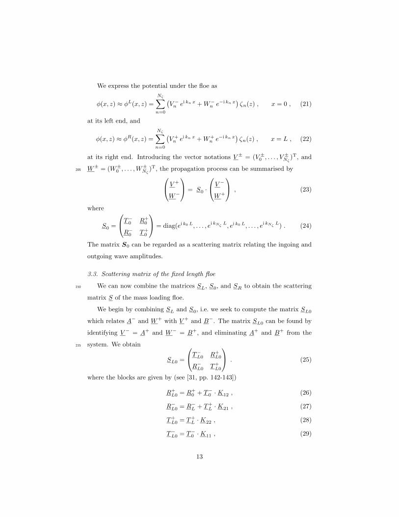
We express the potential under the floe as

φ(x, z) ≈ φL(x, z) =

Nζ∑n=0

(V −n ei kn x +W−

n e−i kn x)ζn(z) , x = 0 , (21)

at its left end, and

φ(x, z) ≈ φR(x, z) =

Nζ∑n=0

(V +n ei kn x +W+

n e−i kn x)ζn(z) , x = L , (22)

at its right end. Introducing the vector notations V ± = (V ±0 , . . . , V

±Nζ

)T, and

W± = (W±0 , . . . ,W

±Nζ

)T, the propagation process can be summarised by205 V +

W−

= S0 ·

V −

W+

, (23)

where

S0 =

T−0 R+

0

R−0 T+

0

= diag(ei k0 L, . . . , ei kNζ L, ei k0 L, . . . , ei kNζ L) . (24)

The matrix S0 can be regarded as a scattering matrix relating the ingoing and

outgoing wave amplitudes.

3.3. Scattering matrix of the fixed length floe

We can now combine the matrices SL, S0, and SR to obtain the scattering210

matrix S of the mass loading floe.

We begin by combining SL and S0, i.e. we seek to compute the matrix SL0

which relates A− and W+ with V + and B−. The matrix SL0 can be found by

identifying V − = A+ and W− = B+, and eliminating A+ and B+ from the

system. We obtain215

SL0 =

T−L0 R+

L0

R−L0 T+

L0

. (25)

where the blocks are given by (see [31, pp. 142-143])

R+L0 = R+

0 + T−0 ·K12 , (26)

R−L0 = R−

L + T+L ·K21 , (27)

T+L0 = T+

L ·K22 , (28)

T−L0 = T−

0 ·K11 , (29)

13

and K11 K12

K21 K22

=

1 −R+L

−R−0 1

−1

·

T−L 0

0 T+0

. (30)

The procedure of combining SL and S0 to form SL0 using (25)–(30) uniquely

defines a binary associative operation , as any two matrices of equal size can

be combined in this way. Specifically, we define SL S0 = SL0. It follows, that220

the scattering matrix of the entire mass loading floe S is

S = SL S0 SR . (31)

3.4. Transmission and reflection coefficients

We are primarily interested in the transmission and reflection coefficients

of the floe. They are given by the amplitudes of the transmitted and reflected

propagating wave modes, normalised by the ingoing wave amplitude (see (9)225

and (10)), i.e.

T = |S0,0| and R = |SNζ+1,0| , (32)

respectively, where Si,j denotes the entry of the matrix S in the (1 + i)th row

and (1 + j)th column.

14

4. Random length scattering

We now randomize the floe length L by writing230

L = L0 + L1 α , (33)

where 0 < L1 < L0, and α is a random variable drawn from some given prob-

ability distribution D constrained to the interval [−1, 1]. The deterministic

boundary value problem described in §3 then becomes a stochastic boundary

value problem. In particular, the reflection coefficient R and the transmission

coefficient T now depend on the random variable α. Our objective is to compute235

the expectation values and variances of R(α) and T (α).

To accomplish this goal we employ the framework of generalised polynomial

chaos (gPC), which is expected to converge significantly faster than the tradi-

tional Monte Carlo (MC) approach [19]. In the MC method the deterministic

problem described in §3 is solved for a large number of randomly selected floe240

lengths and mean and variance are obtained from that solution sample. The

error of this method is known to converge with the inverse square root of the

sample size. In contrast, when the dependence of the solutions on the random

variable(s) is sufficiently smooth, the gPC methods often show exponential con-

vergence behaviour, although there exists no rigorous mathematical proof of245

this, to our knowledge.

The key to the gPC technique is the expansion of the α-dependent quantities

in terms of a particular polynomial basis Pn(α), n ∈ N, which is optimal (in a

sense explained below) for the probability distribution D of α. The polynomials

Pn(α) are constructed, for example using the Gram Schmidt algorithm, to be250

orthonormal with respect to the scalar product

〈f1, f2〉α =

∫ +1

−1

f1(α) f2(α) PDF[D](α) dα , (34)

where PDF[D] is the probability density function of the distribution D. Specif-

ically,

〈Pi, Pj〉α = δij , (35)

15

where δij is the Kronecker delta. For many of the common probability distribu-

tions, however, the corresponding polynomial basis is well established [19]. We255

refer to the Pn(α) as gPC polynomials.

The polynomial basis Pn(α) is optimal in the following sense. Let the

reflection coefficient R(α) be expanded in this basis, that is

R(α) ≈NP∑n=0

Rn Pn(α) , (36)

where we only take a finite number of NP +1 polynomials into account. Then it

can be shown that the truncated expression on the right hand side of (36) not260

only converges to R(α) as NP →∞, but it also minimises the L2 norm error of

any same degree polynomial approximation [19, eq. 5.9].

The family of gPC techniques admits two main branches: stochastic colloca-

tion (SC) methods, and the stochastic Galerkin (SG) scheme. In the following

two subsections we demonstrate both methods by solving the random length265

problem.

4.1. Stochastic collocation method

We first discuss the stochastic collocation (SC) method [19, 32]. This method

is non-intrusive, i.e. it utilizes the deterministic solver described in §3 and is

therefore straightforward to implement.270

The first step is to solve the fixed length scattering problem described in §3

for NC + 1 different floe lengths L = L0 + L1 αm, with m = 0, .., NC .

Setting NC = NP , using the orthonormality condition (35) and the expan-

sion (36) of the reflection coefficient, we find

Rm =

∫ 1

−1

dα PDF[D](α) Pm(α)R(α) ≈NP∑i=0

wi Pm(αi)R(αi) , (37)

where the αi are the roots of PNP+1(α), and wi are the quadrature weights275

for PDF[D]. An efficient way of computing the αi and wi is described in [33].

Alternatively, the expansion (36) could be used to obtain a linear system of

NC + 1 equations in NP + 1 variables, which could then be solved directly or

16

with a least squares method if NP < NC . Both methods perform equally well as

the bulk of the computation time is spent on the evaluations of R(αi). Here we280

choose the quadrature method for its superior robustness and the convenience

that we have to discuss convergence in only one numerical parameter NP .

The orthonormality relation (35) can then be used to find the expectation

E(R) = R0 and variance Var(R) =∑NPn=1R

2n of the reflection coefficient. The

function R(α) = |SNζ+1,0(α)| may not be differentiable at all α, however, due to285

the absolute value in (32), in which case the polynomial approximation converges

poorly. To remedy this possible issue we instead expand the underlying complex

amplitude a(α) = SNζ+1,0(α) into gPC polynomials, i.e.

a(α) =

NP∑n=0

an Pn(α) . (38)

We can then compute the expectation value of R = |a| as

E(R) = E(|a|) =

∫ +1

−1

|a(α)|PDF[D](α) dα , (39)

which can be estimated using numerical integration. Alternatively, one could290

compute the expectation value and variance of logR2 and log T 2. Bennetts and

Squire [31] show that the log-averaged transmission coefficient E(log T 2) of a

single floe gives information about the scattering of an infinite series of floes

whose lengths are uniformly randomly distributed. In §5.4 we show, however,

that these results are not valid for other length distributions and since we are295

concerned with only a single floe we consider the quantities E(R), Var(R), etc.,

which are easier to interpret. We also remark that semi-analytic expressions for

E(T ) and E(R) can be derived if L1 is an integer multiple of the ice covered

propagating wavelength and L is sufficiently large so that the effect of evanes-

cent modes can be neglected (see [34] and references therein). We made sure300

that the E(T ) computed with the semi-analytic expression given in [34] agrees

with our gPC results when these conditions are satisfied.

Note, that orthonormality of the gPC polynomials cannot be used to simplify

17

A-

B-

A+

B+

SL

V-

W-

V+

W+

S0

C-

D-

C+

D+

SR

Figure 3: Separation of the stochastic scattering problem into three sub-problems.

the integral in (39). It can be used to simplify the second moment, however, i.e.305

Var(R) =

∫ +1

−1

|a(α)|2 PDF[D](α) dα− E(R)2

≈NP∑

m,n=0

am a∗n

∫ +1

−1

Pm(α)Pn(α) PDF[D](α) dα− E(R)2

=

NP∑n=0

|am|2 − E(R)2 , (40)

where a∗n is the complex conjugate of an. The results for the transmission

coefficient T (α) follow analogously.

In §5.1 we implement the SC method by expanding the complex amplitudes

underlying the reflection and transmission coefficients into gPC modes.

4.2. Stochastic Galerkin method310

In this section we introduce the stochastic Galerkin (SG) method to solve

the problem of water wave scattering by a floe of random length. In contrast to

the SC method described in §4.1, the SG method does not build upon the de-

terministic solver outlined in §3. Instead, the solution method used to solve the

fixed length problem is amended to account for the dependence of the complex315

wave amplitudes on the random variable α.

Similarly to the fixed length case, we decompose the scattering problem into

three sub-problems, illustrated in figure 3, i.e. (i) scattering from the left edge,

(ii) propagation of the plane wave solutions in the random domain under the

floe, and (iii) scattering from the right edge. As in the fixed length case, each320

process can be described by a scattering matrix.

18

4.2.1. Scattering from the floe’s edges

The solution method of the left edge scattering problem is similar to that

described in §3.1 for the fixed length floe. The potential expansions (11) and (12)

only need to be amended to account for their dependence on the random variable325

α. In the free surface region, only the left-travelling wave amplitudes B− depend

on α as the right-travelling modes are incident from −∞ and therefore do not

depend on the geometry of the floe. In the ice-covered region, both A+ and B+

depend on α. Using the gPC framework, we expand these amplitudes in the

gPC polynomial basis Pi(α). Specifically,330

A+(α) =(A+

0 (α), . . . , A+Nζ

(α))T

=(NP∑i=0

A+0,i Pi(α), . . . ,

NP∑i=0

A+Nζ ,i

Pi(α))T

=(A+

0 · P (α), . . . ,A+Nζ· P (α)

)T, (41)

where A+n , n = 0, . . . , Nζ , are row vectors of length NP + 1 containing the

amplitudes A+n,i and P (α) is the column vector of NP + 1 gPC poynomials.

Similarly, we have

B± =(B+

0 · P (α), . . . ,B+Nζ· P (α)

)T, (42)

where B±n , n = 0, . . . , Nζ , are the row vectors of amplitudes B±

n,i. Note that

we use bold symbols to represent vectors and matrices in the gPC space, as335

opposed to the underlined symbols defined in §3, which represent vectors and

matrices in the vertical mode space. Using this matrix notation, the general

solutions (11) and (12) to Laplace’s equation on the left and right side of the

edge, respectively, become

φ(x, z;α) ≈ φ−(x, z;α)

=

Nζ∑n=0

(A−n e

iκn x +B−n · P (α) e−iκn x

)ςn(z) , x ≤ 0 , (43)

19

on the left (open water) side and340

φ(x, z;α) ≈ φ+(x, z;α)

=

Nζ∑n=0

(A+n e

i kn x +B+n e

−i kn x)· P (α) ζn(z) , x ≥ 0 , (44)

on the right (ice-covered) side.

The matching of the potential and normal velocity at x = 0 can be done

for each gPC mode independently. The scattering matrix of the left edge can

therefore be expressed directly in terms of the reflection and transmission block

components of the scattering matrix SL given in (17) and (18) for the fixed345

length problem. Specifically, we can write the mapping of wave mode amplitudes

on either side of the edge as

A+ = T−L ·A

− +R+L ·B

+ , (45)

B− = R−L ·A

− + T+L ·B

+ . (46)

where the vectors A+ = (A+0 , . . . ,A

+Nζ

)T and B± = (B±0 , . . . ,B

±Nζ

)T have

length (Nζ + 1)(NP + 1).

The blocks T±L and R±

L of SL must also be amended to operate on the prod-350

uct space of vertical and gPC modes, while leaving the gPC modes unaffected.

Therefore the matrices T+L and R+

L are given by

R+L = R+

L ⊗ 1 and T+L = T+

L ⊗ 1 , (47)

where 1 is the identity matrix of dimension (NP + 1) × (NP + 1). The op-

eration ⊗ is the Kronecker product, which is the matrix representation of the

tensor product. Effectively, every entry (R+L)ij is replaced by the diagonal block355

(R+L)ij 1 and the same is done for T+

L . Since A− does not depend on α, it can

only influence the zeroth order term P0(α) = 1 in the gPC expansions of A+

and B−. Therefore, the matrices R−L and T−

L acting on A− are expressed as

R−L = R−

L ⊗ e0 and T−L = T−

L ⊗ e0 , (48)

where e0 is the unit column vector in the space of gPC polynomials which

corresponds to P0(α) = 1, with size (NP + 1). Effectively, every entry (R−L )ij360

20

is replaced with the column vector ((R−L )ij , 0, . . . , 0)T and the same is done for

T−L . The scattering matrix SL of the left edge can be assembled from these four

blocks, i.e. A+

B−

= SL ·

A−

B+

=

T−L R+

L

R−L T+

L

·A−

B+

. (49)

It relates the gPC modes of the wave amplitudes A−n and B+

n (α) to the gPC

modes of the wave amplitudes A+n (α) and B−

n (α).365

As in the fixed length case, the symmetry of the problem allows us to con-

struct the right-edge scattering matrix SR from the block components of SL.

4.2.2. Wave propagation in a random domain

In §3.2 we constructed the matrix S0, which describes the phase change of

the wave modes between the two edges x = 0 and x = L. We now seek a370

mapping S0 describing the phase change of the wave modes when the boundary

x = L(α) is only given in terms of the probability distribution of α.

To that end, we follow Xiu and Tartakovsky [35] by first transforming the

deterministic governing equations with a random boundary into stochastic equa-

tions with a fixed boundary. This is accomplished by expressing the Laplace375

equation (1) in a new α-dependent coordinate system (x, z), defined by

x(x;α) = s(α)x with s(α) =L0

L0 + L1 α, (50)

which is chosen such that the left and right floe edges always have the coordi-

nates x = 0 and x = L0, respectively. In this new coordinate system, Laplace’s

equation (1) becomes

−s2(α) ∂2xφ = ∂2zφ , (51)

while the ice-covered surface and sea floor boundary conditions (6) and (7)380

remain unchanged. In the horizontal direction, the solution must be matched

21

in φ and ∂xφ to

φ(x, z;α) ≈ φL(x, z;α)

=

Nζ∑n=0

(V −n e

i kn x +W−n e

−i kn x)· P (α) ζn(z) , x = 0 , (52)

at x = x = 0, which is analogous to equation (21) in the fixed length problem,

and to

φ(x, z;α) ≈ φR(x, z;α)

=

Nζ∑n=0

(V +n e

i kn x +W+n e

−i kn x)· P (α) ζn(z) , x = L , (53)

at x = L (or equivalently x = L0), analogous to (22). We introduced the row385

vectors V ±n and W±

n of length NP +1 containing the gPC coefficients of V ±n (α)

and W±n (α) for each vertical mode n = 0, . . . , Nζ .

To find the general solution of the stochastic Laplace equation (51), we

separate variables by invoking the ansatz

φ(x, z;α) = ζ(z)ϕ(x;α) . (54)

The vertical solutions ζn are the same as for the deterministic problem, given390

by equation (14). In the horizontal direction we obtain

s2(α) ∂2xϕ(x;α) = −k2 ϕ(x, α) . (55)

We expand ϕ in the gPC polynomial basis

ϕ(x;α) ≈NP∑j=0

ξj(x)Pj(α) , (56)

where the infinite series has been truncated to contain NP +1 terms. Substitut-

ing (56) into equation (55), dividing by s2(α), and projecting on Pi using the

gPC scalar product (34), results in395

∂2xξi(x) = −k2NP∑j=0

ξj(x) 〈Pi, s−2 Pj〉α , (57)

22

where we have used the orthonormality (35) of the gPC polynomials. We define

the row vector ξ of length NP + 1 and the square matrix M of size (NP + 1)×

(NP + 1), with entries given by ξ · ei = ξi(x), and eTi ·M · ej = 〈Pi, s−2 Pj〉α,

respectively, where ei corresponds to the ith unit vector in the gPC standard

basis. This allows us to rewrite (57) in matrix form as400

∂2x ξ = −k2 ξ ·M . (58)

The matrix M is real and symmetric, so there exists a unitary matrix U such

that M = U · /M ·U−1, where /M is diagonal. Thus, we can write

∂2x ξ = −k2 ξ ·U · /M ·U−1 , (59)

∂2x ξ ·U = −k2 ξ ·U · /M , (60)

∂2xX = −k2 X · /M , (61)

where we define the row vector X = ξ · U of length NP + 1. Since /M is

diagonal, this is a system of independent ordinary differential equations with

general solution405

ξ =

(V 0 · exp (i k

√/M x) +W 0 · exp (−i k

√/M x)

)·U−1 , (62)

where V 0 and W 0 are now vectors of length NP + 1 and where we have used

the definition of X. The general solution to (51) can therefore be approximated

by

φ(x, z;α) ≈ φ0(x, z;α) =

Nζ∑n=0

ζn(z) ξn(x) · P (α) (63)

=

Nζ∑n=0

ζn(z)

(V 0n · exp (i knG x) +W 0

n · exp (−i knG x)

)·U−1 · P (α) ,

where we have introduced G =√/M .

We are now in a position to construct the random phase change matrix S0410

by matching the general solution (63) under the floe to the solutions (52) and

(53) at x = 0 and x = L. Applying the four matching conditions

φL(x, z;α)|x=0 = φ0(x, z;α)|x=0 , (64)

φ0(x, z;α)|x=L0= φR(x, z;α)|x=L , (65)

23

and

∂xφL(x, z;α)|x=0 = s(α) ∂xφ

0(x, z;α)|x=0 , (66)

s(α) ∂xφ0(x, z;α)|x=L0 = ∂xφ

R(x, z;α)|x=L , (67)

and projecting onto the vertical and gPC modes, we obtain the four matrix

equations415

(V −n +W−

n ) = (V 0n +W 0

n) ·U−1 , (68)

(V +n +W+

n ) = (V 0n exp (i knGL0) +W 0

n exp (−i knGL0)) ·U−1 , (69)

(V −n −W

−n ) ·N = (V 0

n −W0n) ·G ·U−1 , (70)

(V +n −W

+n ) ·N = (V 0

n exp (i knGL0)−W 0n exp (−i knGL0)) ·G ·U−1 .

(71)

where we have defined the (NP + 1) × (NP + 1) matrix N with components

eTi ·N · ej = 〈Pi, s−1 Pj〉α. Eliminating V 0n and W 0

n from equations (68)–(71),

we obtain the mapping V +

W−

= S0 ·

V −

W+

, (72)

where the random phase change matrix S0 is defined by

S0 =

T−0 R+

0

. . .. . .

T−Nζ

R+Nζ

R−0 T+

0

. . .. . .

R−Nζ

T+Nζ

. (73)

The blocks T±n and R±

n are given by420

R±n = Cn · (E−1

n · F− − F− · (F+)−1 ·En · F+) , (74)

T±n = Cn · (F+ − F− · (F+)−1 · F−) , (75)

24

where

F± = U−1 ±G ·U−1 ·N−1 , (76)

Cn =(E−1n F+ − F− · (F+)−1 ·En · F−

)−1

, (77)

En = exp (i knGL0) . (78)

The matrix S0 maps the gPC modes of the amplitudes of the wave modes

travelling into the covered region to the gPC modes of the amplitudes of the

wave modes travelling out of the covered region, where the effect of the floe edge

has not yet been considered. It therefore describes the random phase change of425

the waves under the floe.

4.2.3. The Random Scattering Matrix

The procedure described in §3.3 to combine scattering matrices remains

unchanged in the random length case. Using the operation defined in §3.3 we

express the scattering matrix of the random length ice floe as430

S = SL S0 SR , (79)

which has dimension 2 (Nζ+1)(NP +1)×2 (Nζ+1). It relates the α-independent

amplitudes of the ingoing waves to the α-dependent amplitudes of the outgoing

waves (see figure 3), i.e. C+

B−

= S ·

A−

D+

. (80)

We use (39) and (40) to calculate the expectation and variance, respectively,

of the absolute value of any complex quantity obtained from the SG method. In435

particular, applying these formulae for the travelling vertical mode amplitudes

C+0 (α) = C+

0 · P and B−0 (α) = B−

0 · P gives the statistical central moments of

the transmission and reflection coefficients, respectively.

25

5. Results

We devise a number of numerical tests to establish the performance of the440

two SC methods described in §4.1 and the SG method described in §4.2, in

comparison to the Monte Carlo (MC) approach. The parameters L0 = 30 m,

L1 = 10 m, H = 100 m, h = 2 m, and ω = 2π/5 Hz are fixed for all of the

following simulations. This implies, that the travelling wave modes in the open

water and floe covered domains have wavelength λ0 = 2π/κ0 = 39 m, and445

λice0 = 2π/k0 = 28 m, respectively. We also set the number of evanescent

vertical modes to Nζ = 5 and compute the solution of the matching problem at

the floe edges with a sufficient level of certainty to ensure that the transmission

coefficient T has converged to six digits of accuracy.

Throughout this article we consider two possible choices for the distribution450

D of α: (i) the uniform distribution U on the interval [-1,1], which we adopt

because of its simplicity, and (ii) a beta distribution that has been transformed

to be non-zero on the interval [-1,1]. We chose the latter distribution because

its probability density function resembles that of a normal distribution while it

converges continuously to zero as α → ±1. Other probability distributions on455

[−1, 1] could be used instead. The PDFs of U and B are given by

PDF[U ](α) =1

2, (81)

and

PDF[B](α) =21−2m

(1− α2

)m−1

B(m,m)

∣∣∣∣m=10

=230945

131072

(1− α2

)9, (82)

respectively, where B(m,m) is the beta function. Their graphs are shown in

the top panel of figures 4 and 5, respectively.

The gPC polynomials corresponding to U and B, as defined by (34) and460

(35), are

Pn(α) =√

2n+ 1 P(0,0)n (α) , (83)

and

Pn(α) =

√(2n+ 19)n! (n+ 18)!

2√

230945 (n+ 9)!P(9,9)n (α) , (84)

26

respectively, for n = 0, . . . , NP , and where P(i,j)n (α) are the Jacobi polynomials

of degree n [19]. It should be noted that for i = j = 0 the Jacobi polynomials

P(i,j)n (α) reduce to the Legendre polynomials for all non-negative integers n.465

First, we illustrate how the probability distribution R(D) of the output re-

flection coefficient R is related to the probability distribution D of the input α.

Figures 4 and 5 show the reflection coefficient as a function of the parameter

α (central panel), which does not depend on the choice of the distribution D.

Thus, we constructed the graph by computing several solutions R(α) for differ-470

ent α, using the procedure described in §3. The SC and SG methods provide

analytic expressions approximating the function R(α). Via (39) and (40) they

also provide the expectation E(R) and (taking the square root) the standard

deviation Var(R)1/2

, which are displayed as error bars on the right panels of

the two figures.475

The right panels of figures 4 and 5 also show an approximation to PDF[R(D)].

To compute the latter, we subdivided the range of R(α) into 100 intervals

[rn, rn+1], n = 0, · · · , 99. For each interval we then estimated the probability

that rn ≤ R < rn+1 by numerically integrating PDF[D](α) over the α-intervals

for which R(α) satisfies this condition. Consequently, the extrema of PDF[D](α)480

correspond to discontinuities in PDF[R(D)](R). These discontinuities are only

prominent if PDF[D](α) is large at the corresponding extremum, however. Con-

sider for example the discontinuity at R ≈ 0.16 in figure 4, which is generated

from the endpoint minimum of R(α) at α = 1. This discontinuity is not visible

in figure 5, because the PDF of the beta distribution vanishes with α→ 1. We485

also notice, that PDF[R(U)](R) is skewed towards large R, as most points of

the graph of R(α) lie in the upper half of the range of R(α) and all points are

equally weighted by the uniform distribution of α. The PDF[R(B)](R) is more

evenly distributed, because the beta distribution gives more weight to small

R(α). Consequently, the expectation value of R is lower for α ∼ B than it is for490

α ∼ U .1

1We use the standard notation in statistics where ∼ stands for “has the probability distri-

27

-1 -0.5 0 0.5 10

0.05

0.1

0.15

0.2

0.25

0.3

0

0.5

1

0 0.05

0

0.05

0.1

0.15

0.2

0.25

0.3

0.35

α

R(α)

PDF[](α)

PDF[R()](R)

Figure 4: Transformation of the probability distribution. The top panel shows the uniform

probability density function for the random length parameter α ∼ U . The central panel shows

the reflection coefficient R as a function of α. The right panel shows the histogram of the

probability distribution of R(U). The point and error bar represent the expected R ± its

standard deviation as computed by the stochastic Galerkin method.

-1 -0.5 0 0.5 10

0.05

0.1

0.15

0.2

0.25

0.3

0

1

2

0 0.01

0

0.05

0.1

0.15

0.2

0.25

0.3

0.35

α

R(α)

PDF[ℬ](α)

PDF[R(ℬ)](R)

Figure 5: Same as figure 4, but with α following the transformed beta distribution B.

28

D method E(T ) Var(T ) E(R) Var(R) timing in s

U SC 10 9 17 14 0.90

U SG 9 9 16 13 0.76

B SC 7 7 14 10 0.82

B SG 7 6 13 9 2.2

Table 1: Numerical parameters and computation times of the two gPC methods. The integers

give the smallest number of gPC polynomials N = NP (= NC) necessary to achieve six digit

accuracy in the quantity of the respective column. The timings have been estimated using

the maximum NP in the respective row, such that all quantities are computed with at least

six digit accuracy. The Monte Carlo (MC) method did not converge to comparable accuracy

(see figures 9 and 10) after 60 s and therefore is not included in the table.

5.1. Stochastic collocation method

We implement the SC method by expanding the complex amplitudes, cor-

responding to the reflection and transmission coefficients, into NP gPC modes.

Figure 6 shows the error of the SC method for various numbers of collocation495

points N = NC = NP . The case α ∼ U is shown on the left side (panel a),

and the case α ∼ B is shown on the right side (panel b). For both distributions

of α the computed central moments of the transmission coefficient T and the

reflection coefficient R converge exponentially, at least up to some N = Ncrit.

For the expectation and variance of T we find Ncrit = 16 for both distributions500

of α. Beyond Ncrit the error ∆ increases exponentially (at a slow rate) when

α ∼ U and stays constant at ∆ ≈ 10−13 when α ∼ B. For the expectation and

variance of R we find Ncrit ≥ 25 when α ∼ U (not shown) and Ncrit = 20 when

α ∼ B. In the latter case the error ∆ stays roughly constant at ∆ ≈ 5× 10−10

for N ≥ Ncrit.505

5.2. Stochastic Galerkin method

Figure 7 illustrates the convergence of the SG method. When α ∼ U the

central moments of R(U) and T (U) converge exponentially in expectation and

bution of”.

29

5 10 15 20 25

10-18

10-13

10-8

0.001

number of collocation points N = NC + 1 = NP + 1

Δ=|f(N

+1)

-f(

N)|

(a )

5 10 15 20 25

10-18

10-13

10-8

0.001

number of collocation points N = NC + 1 = NP + 1

Δ=|f(N

+1)

-f(

N)|

(b)

Figure 6: Estimated accuracy of the SC method. Successive differences in transmission

expectation (blue circles), transmission variance (green squares), reflection expectation (red

diamonds), and reflection variance (orange triangles), as the number of gPC modes and col-

location points N = NC = NP is increased. The random variable α follows the uniform

distribution U in panel (a), and the transformed beta distribution B in panel (b). Horizon-

tal dashed and dash-dotted lines indicate the convergence goal 10−6 and machine precision

∼ 10−16, respectively.

30

5 10 15 20 25

10-18

10-13

10-8

0.001

number of gPC modes N = NP + 1

Δ=|f(N

+1)

-f(

N)|

(a )

5 10 15 20 25

10-18

10-13

10-8

0.001

number of gPC modes N = NP + 1

Δ=|f(N

+1)

-f(

N)|

(b)

Figure 7: Same as figure 6, but for the SG method.

variance. When α ∼ B the exponential convergence of the central moments of

R(B) stops at 10−13 with N = Ncrit = 19. For larger N the large numbers510

occurring in the expression (84) result in an error increase. For N > 25 ill-

conditioned matrices lead to a breakdown of the SG algorithm.

We consider the solution converged, if all solutions computed with larger NP

differ from it by less than 10−6. The number of gPC modes NP + 1 necessary

for six digits of accuracy is given in table 1 for each quantity of interest.515

5.3. Comparison of performances

Both gPC methods show exponential convergence up to some N = Ncrit,

thereby achieving at least nine digits of precision in the central moments of the

reflection and transmission coefficients.

Figure 8 shows the exponential convergence rates γ against Ncrit, assuming520

the error ∆ ∝ exp(−γ NP ) for all NP ≤ Ncrit. In every case γ lies between

0.6 and 1.8. We always find γ and Ncrit for the expectation value of a quantity

close to the γ and Ncrit for its variance. This is expected, as expectation and

variance are both computed from the same gPC expansions using equations

(39) and (40). Computation of R generally converges slower. This is also not525

surprising, as the value of R is small compared to the value of T , which implies

31

(a )

15 20 25 30

0.75

1.

1.25

1.5

1.75

Ncrit

exp.

conv

erge

nce

rate

T

R

(b)

15 20 25 30

0.75

1.

1.25

1.5

1.75

Ncrit

exp.

conv

erge

nce

rate

T

R

Figure 8: Exponential convergence rates of the gPC methods againstNcrit, where convergence

is exponential for all NP ≤ Ncrit. The two panels (a) and (b) contain results for α ∼ U and

α ∼ B, respectively. Expectation values of T (above 1) and R (below 1), computed with the SG

(blue rectangles) and SC (red circles) method are connected by a line with the corresponding

variances, indicated by a cross. Convergence has not been tested beyond NP = 25.

that high precision is needed to achieve the same accuracy. Overall, the SC and

SG methods show similar convergence properties, except when we compute the

moments of T with α ∼ U , where the SG method converges to much higher

precision (larger Ncrit) than the SC method. This may change, however, with530

different period, floe thickness, or water depth settings.

We estimated average computation times using a machine with an IntelR

CoreTM i7-3517U CPU (2.4 GHz) and 10 GB RAM (WolframMarkTM bench-

mark 0.78). The timings for the gPC methods are listed in table 1.

When α ∼ U the SC and SG methods show similar performance, while when535

α ∼ B the SG method is significantly slower.

One has to keep in mind, however, that the SG method returns much more

information than the SC methods. Specifically, it gives an approximation to

the functional dependence of all outgoing complex amplitudes on the random

parameter α (see equation (80)). Furthermore, formulae (39) and (40) can be540

used, respectively, to compute the expectation and variance of the outgoing

32

transmission reflectionun

iform

0.9674 0.9676 0.9678 0.233 0.234 0.235

beta

0.9829 0.983 0.9831 0.9832 0.9833 0.1555 0.156 0.1565 0.157 0.1575

Figure 9: Expectation values, as predicted by the SG (blue), MC (green), and SC (red)

methods (top to bottom in each panel). The intervals signify the accuracies with which these

results were obtained.

transmission reflection

unifo

rm

0.000354 0.000356 0.000358 0.00855 0.0086 0.00865 0.0087 0.00875 0.0088

beta

0.000254 0.000256 0.000258 0.00026 0.000262 0.0087 0.00875 0.0088 0.00885

Figure 10: Same as figure 9, but for variances.

evanescent wave mode amplitudes.

Figures 9 and 10 show, for the two probability distributions U and B, the

expectations and variances of R and T , respectively, computed with the three

different methods, i.e. SG, SC, and MC. In the MC approach we compute the545

R and T for 104 values of α which are sampled from either U or B. This takes

about 60 s. Expectation and variance are estimated from this sample. The

displayed interval is defined as mean ± standard deviation, estimated from 10

individual MC runs with different random seeds, each of which takes about 60 s.

The results of all three methods are compatible within their respective accu-550

racies. That is, six digits for all gPC methods and significantly larger intervals

for the MC method, despite its runtime being more than 20 times greater than

the runtime of any of the gPC methods.

33

5.4. Uniform vs. beta distribution

The good performance of the gPC methods allows us to compute results for555

a large variety of parameters, such as wave frequency and floe thickness. Each

of the two panels of figure 11 shows an overlay of two contour plots in the space

of these two parameters. The shaded contours in the background represent the

reflection coefficient R, computed for a fixed floe length L = 38 m.

We note that the minima (dark areas) correspond to regions where the floe560

length is commensurable with the ice covered water wavelength λice0 < λ0, where

reflection is especially low.

The white dashed lines indicate the contours of the expected reflection co-

efficient E(R), assuming either α ∼ U (left panel a), or α ∼ B (right panel

b). These contours are computed by running the SC method to calculate E(R)565

for more than 1000 parameter pairs, where we ensured that each computation

converged to at least three digits of accuracy. We chose L0 = 38 m (as for the

fixed length countours in the background) and L1 = 20 m throughout. One

can clearly see that the E(R) contours are very similar to those of R when α

follows the transformed beta distribution B, which is peaked around L = L0. In570

contrast, when α follows a uniform distribution the E(R) contours are “smeared

out”.

The discrepancy in E(R) between the two distributions is an important ob-

servation. For instance, when Bennetts and Squire [31] calculate the expected

transmission of an array of ice floes of random lengths, they assume the floe575

lengths to be uniformly distributed, whereas real ice floe sizes are believed to

follow a power law distribution [17]. Figure 11 shows that this can make a sig-

nificant difference. Although our results were computed for the mass loading

model, there is no reason to expect this fact to change when e.g. elasticity is

included in the floe model.580

34

0.6 0.7 0.8 0.9 1.0 1.1 1.2

1

2

3

4

5

λ0 = 2 L0λ0 = 4 L0

frequency ω in Hertz

thic

knes

sh

inm

eter

s

(a)

0.6 0.7 0.8 0.9 1.0 1.1 1.2

1

2

3

4

5

λ0 = 2 L0λ0 = 4 L0

frequency ω in Hertz

thic

knes

sh

inm

eter

s

(b)

Figure 11: Contours of R(2π/ω, h) (shaded) overlayed with contours of E[R](2π/ω, h) (white

dashed lines) for (a) α ∼ U and (b) α ∼ B. The fixed length result R is computed for

L = 38 m. For the expectation values we assume the same mean length, i.e. L0 = 38 m and

vary by L1 = 20 m. The water depth is H = 1000 m throughout.

35

6. Conclusions

In the present study, we described three different numerical methods to

solve the scattering problem of water waves from an ice floe modelled as a

layer of mass loading material of random length L, where L = L0 + L1 α and

α ∈ [−1, 1] follows either a uniform or a transformed beta distribution. Two of585

the methods investigated belong to the family of generalised polynomial chaos

(gPC) techniques. Specifically, these are a stochastic collocation method (SC)

and a stochastic Galerkin method (SG). We also implemented a Monte Carlo

technique (MC) for comparison.

Both gPC methods rely on a polynomial expansion of the relevant quanti-590

ties in the random variable. While the SC method is non-intrusive and only

post-processes results computed with the deterministic solver, the SG method

generalises the equations characterising the system to account for the extra

random dimension.

The gPC methods were shown to outperform MC significantly. Specifically,595

they exhibit exponential convergence, while MC converges only with the inverse

square root of the sample size. As a result, the gPC methods achieve six digit

accuracy within less than 3 s (usually less than 1 s), while MC reaches only

comparably low accuracy after 60 s.

Compared to each other, the gPC methods show similar performance. Which600

method is faster depends on the length distribution considered. Specifically, we

found that with α ∼ U the SG method is slightly faster, while with α ∼ B it is

significantly slower than SC.

In contrast to the SG method, the derivation and implementation of the SC

method is straightforward. Moreover, the SC method can be used to compute605

the moments of the evanescent amplitudes as well if required, and therefore does

not have any disadvantage compared to the SG method which always calculates

the complete probabilistic scattering matrix. In conclusion, the simplicity and

superior performance of the SC method makes it more suitable for most appli-

cations.610

36

We finally used the SC method to compute how the expected reflection

coefficient depends on the wave period and floe thickness. This is an important

result, as it suggests that the distribution of floe sizes present in a field of sea ice

floes will be vitally important to the manner in which ocean waves are scattered.

The authors have generalised this study to floating elastic plates (not pre-615

sented here).

The gPC framework can also be applied to non-linear problems and geome-

tries with several random variables, although the latter case is a major challenge

in the development of gPC which is an active field of research.

37

Appendix A. Scattering from the beam’s edge620

In this appendix we briefly discuss the procedure we follow to match the

plane wave solutions on either side of the floe’s edge.

The vertical modes ςn and ζn defined in (13) and (14), respectively, are

orthogonal with respect to the scalar product

〈f1, f2〉z =

∫ 0

−Hf1(z) f2(z) dz , (A.1)

that is625

〈ςm, ςn〉z = δmn ‖ςm‖ (A.2)

〈ζm, ζn〉z = δmn ‖ζm‖ (A.3)

where

‖ςm‖ =κmH sech2(κmH) + tanh (κmH)

2κm(A.4)

‖ζm‖ =kmH sech2(kmH) + tanh (kmH)

2 km. (A.5)

We follow [26] and define an auxiliary function

u(z) = ∂xφ−(x, z)|x=0 = ∂xφ

+(x, z)|x=0 , (A.6)

thereby utilizing the condition of matching horizontal fluid velocities. By pro-

jecting on the respective vertical modes, we can express the amplitudes A+n and

B−n in terms of u:630

A+n = B+

n +〈ζn, u〉zi kn ‖ζn‖

, (A.7)

B−n = A−

n −〈ςn, u〉ziκn ‖ςn‖

. (A.8)

Matching the potentials

φ−(x, z) = φ+(x, z) , x = 0 , (A.9)

38

and using (11), (12), (A.7), and (A.8), we obtain

2 iκlA−l −

Nmatch∑n=0

2 iκl‖ςl‖〈ςl, ζn〉z B+

n

=

Nmatch∑n,m=0

(δln δnm +

κl‖ςl‖〈ςl, ζn〉z

1

kn ‖ζn‖〈ζn, ςm〉z

)um , (A.10)

where we have expanded u(z) =∑Nmatch

m=0 um ςm(z). Note, that we use Nmatch

instead of Nζ , where Nmatch Nζ so that the matching problem is solved with

high accuracy. Later on we truncate the resulting matrices such that only Nζ635

evanescent modes are taken into account for further computations.

Defining the (Nζ + 1)× (Nζ + 1) matrix Z with entries eTi ·Z · ej = 〈ςi, ζj〉z,

as well as the vector u = (u0, . . . , uNζ )T, we can write (A.10) in matrix form as

follows

u = 2 i(

1 +K− · (ζ−)−1 · Z · (K+)−1 · (ζ+)−1 · ZT)−1

·(K− ·A− −K− · (ζ−)−1 · Z ·B+

), (A.11)

where K+, K−, ζ+ and ζ− are diagonal matrices with the diagonal elements640

ki, κi, ‖ζi‖, and ‖ςi‖, respectively. In this notation, equations (A.7) and (A.8)

become

A+ = B+ − i (K+)−1 · (ζ+)−1 · ZT · u (A.12)

B− = A− + i (K−)−1 · u . (A.13)

Comparing this to (19) we identify the reflection and transmission matrices

T− = 2 (K+)−1 · (ζ+)−1 · ZT ·(...)−1

·K− (A.14)

R+ = 1− 2 (K+)−1 · (ζ+)−1 · ZT ·(...)−1

·K− · (ζ−)−1 · Z (A.15)

R− = 1− 2 (K−)−1(...)−1

·K− (A.16)

T+ = 2 (K−)−1(...)−1

·K− · (ζ−)−1 · Z , (A.17)

where (...)−1

=(

1 +K− · (ζ−)−1 · Z · (K+)−1 · (ζ+)−1 · ZT)−1

,

39

as in equation (A.11).645

For our analysis we solve the matching problem with Nmatch = 100 and

then truncate the sizes of the resulting matrices such that only Nζ = 5 evanes-

cent modes are considered. This ensures that the transmission coefficient T is

computed with six digits of accuracy.

Acknowledgements650

J.E.M.M. was supported by a University of Otago Postgraduate Scholar-

ship. F.M. and V.A.S. were supported by the Office of Naval Research De-

partmental Research Initiative “Sea State and Boundary Layer Physics of the

Emerging Arctic Ocean” (award N00014-131-0279), the EU FP7 grant (SPA-

2013.1.1-06), and the University of Otago. We also thank Stuart Hawkins for655

interesting discussions during the KOZWaves conference, as well as the review-

ers for their constructive comments. The source code necessary to reproduce

the figures presented in this article is available from the authors upon request

(jmosig@maths.otago.ac.nz).

References660

[1] V. A. Squire, Synergies Between VLFS Hydroelasticity and Sea Ice Re-

search, Int. J. Offshore Polar 18 (3) (2008) 1–13.

[2] E. Watanabe, T. Utsunomiya, C. M. Wang, Hydroelastic analysis of

pontoon-type VLFS: a literature survey, Eng. Struct. 26 (2) (2004) 245–256.

doi:10.1016/j.engstruct.2003.10.001.665

[3] V. A. Squire, Of ocean waves and sea-ice revisited, Cold Reg. Sci. Technol.

49 (2) (2007) 110–133. doi:10.1016/j.coldregions.2007.04.007.

[4] M. Meylan, V. A. Squire, The response of ice floes to ocean waves, J.

Geophys. Res. - Oceans 99 (C1) (1994) 891–900. doi:10.1029/93JC02695.

[5] I. V. Sturova, Oblique incidence of surface waves on an elastic plate, J.670

Appl. Mech. Tech. Phys. 40 (4) (1999) 604–610. doi:10.1007/BF02468434.

40

[6] A. I. Andrianov, A. J. Hermans, The influence of water depth on the hy-

droelastic response of a very large floating platform, Mar. Struct. 16 (5)

(2003) 355–371. doi:10.1016/S0951-8339(03)00023-6.

[7] R. E. Taylor, Hydroelastic analysis of plates and some approximations, J.675

Eng. Math. 58 (1-4) (2006) 267–278. doi:10.1007/s10665-006-9121-7.

[8] T. D. Williams, V. A. Squire, Oblique scattering of plane flexuralgravity

waves by heterogeneities in seaice, Philos. T. Roy. Soc. A 460 (2052) (2004)

3469–3497. doi:10.1098/rspa.2004.1363.

[9] L. G. Bennetts, N. R. T. Biggs, D. Porter, A multi-mode approximation680

to wave scattering by ice sheets of varying thickness, J. Fluid. Mech. 579

(2007) 413–443. doi:10.1017/S002211200700537X.

[10] M. J. A. Smith, M. H. Meylan, Wave scattering by an ice floe of variable

thickness, Cold Reg. Sci. Technol. 67 (12) (2011) 24–30. doi:10.1016/j.

coldregions.2011.03.003.685

[11] M. H. Meylan, V. A. Squire, Response of a circular ice floe to ocean

waves, J. Geophys. Res. - Oceans 101 (C4) (1996) 8869–8884. doi:

10.1029/95JC03706.

[12] M. A. Peter, M. H. Meylan, H. Chung, Wave Scattering By a Circular

Elastic Plate In Water of Finite Depth: A Closed Form Solution, Int. J.690

Offshore Polar Eng. 14 (02).

[13] F. Montiel, L. G. Bennetts, V. A. Squire, F. Bonnefoy, P. Ferrant, Hy-

droelastic response of floating elastic discs to regular waves. Part 2. Modal

analysis, J. Fluid. Mech. 723 (2013) 629–652. doi:10.1017/jfm.2013.124.

[14] L. G. Bennetts, N. R. T. Biggs, D. Porter, Wave scattering by an axisym-695

metric ice floe of varying thickness, IMA J. Appl. Math. 74 (2) (2009)

273–295. doi:10.1093/imamat/hxn019.

41

[15] M. H. Meylan, Wave response of an ice floe of arbitrary geometry, J. Geo-

phys. Res. - Oceans 107 (C1). doi:10.1029/2000JC000713.

[16] L. G. Bennetts, T. D. Williams, Wave scattering by ice floes and polynyas700

of arbitrary shape, J. Fluid. Mech. 662 (2010) 5–35. doi:10.1017/

S0022112010004039.

[17] T. Toyota, C. Haas, T. Tamura, Size distribution and shape properties of

relatively small sea-ice floes in the Antarctic marginal ice zone in late win-

ter, Deep Sea Research Part II: Topical Studies in Oceanography 58 (910)705

(2011) 1182–1193. doi:10.1016/j.dsr2.2010.10.034.

[18] Z. Lu, D. Zhang, A Comparative Study on Uncertainty Quantification for

Flow in Randomly Heterogeneous Media Using Monte Carlo Simulations

and Conventional and KL-Based Moment-Equation Approaches, SIAM J.

Sci. Comput. 26 (2) (2004) 558–577. doi:10.1137/S1064827503426826.710

[19] D. Xiu, Numerical methods for stochastic computations: a spectral method

approach, Princeton University Press, Princeton, N.J, 2010.

[20] M. Ganesh, S. C. Hawkins, Scattering by stochastic boundaries: hybrid

low- and high-order quantification algorithms, ANZIAM J. 56 (0) (2016)

312–338, 00000. doi:10.0000/anziamj.v56i0.9313.715

[21] X. Wan, G. E. Karniadakis, An adaptive multi-element generalized polyno-

mial chaos method for stochastic differential equations, J. Comput. Phys.

209 (2) (2005) 617–642. doi:10.1016/j.jcp.2005.03.023.

[22] O. P. Le Matre, O. M. Knio, H. N. Najm, R. G. Ghanem, Uncertainty

propagation using WienerHaar expansions, J. Comput. Phys. 197 (1) (2004)720

28–57. doi:10.1016/j.jcp.2003.11.033.

[23] M. Weitz, J. B. Keller, Reflection of water waves from floating ice in water

of finite depth, Commun. Pur. Appl. Math. 3 (3) (1950) 305–318.

42

[24] P. Wadhams, B. Holt, Waves in frazil and pancake ice and their detection in

Seasat synthetic aperture radar imagery, J. Geophys. Res. - Oceans 96 (C5)725

(1991) 8835–8852. doi:10.1029/91JC00457.

[25] J. M. Gere, S. P. Timoshenko, Mechanics of Materials, Springer US, Boston,

MA, 1991.

[26] T. D. Williams, R. Porter, The effect of submergence on the scattering

by the interface between two semi-infinite sheets, J. Fluid. Struct. 25 (5)730

(2009) 777–793. doi:10.1016/j.jfluidstructs.2009.02.001.

[27] T. D. Williams, V. A. Squire, Scattering of flexuralgravity waves at the

boundaries between three floating sheets with applications, J. Fluid Mech.

569 (2006) 113–140. doi:10.1017/S0022112006002552.

[28] C. M. Linton, H. Chung, Reflection and transmission at the ocean/sea-735

ice boundary, Wave Motion 38 (1) (2003) 43–52. doi:10.1016/

S0165-2125(03)00003-9.

[29] C. Fox, V. A. Squire, On the oblique reflexion and transmission of ocean

waves at shore fast sea ice, Philos. T. Roy. Soc. A 347 (1682) (1994) 185–

218. doi:10.1098/rsta.1994.0044.740

[30] F. Montiel, L. G. Bennetts, V. A. Squire, The transient response of floating

elastic plates to wavemaker forcing in two dimensions, Journal of Fluids and

Structures 28 (2012) 416–433. doi:10.1016/j.jfluidstructs.2011.10.

007.

[31] L. G. Bennetts, V. A. Squire, On the calculation of an attenuation coeffi-745

cient for transects of ice-covered ocean, Proc. R. Soc. A 468 (2137) (2012)

136–162. doi:10.1098/rspa.2011.0155.

[32] O. M. Knio, O. P. Le Maitre, Uncertainty propagation in CFD using poly-

nomial chaos decomposition, Fluid Dyn. Res. 38 (9) (2006) 616–640.

43

[33] G. H. Golub, J. H. Welsch, Calculation of Gauss quadrature rules, Math.750

Comp. 23 (106) (1969) 221–230. doi:10.1090/S0025-5718-69-99647-1.

[34] A. L. Kohout, M. H. Meylan, An elastic plate model for wave attenuation

and ice floe breaking in the marginal ice zone, J. Geophys. Res. 113 (C9)

(2008) C09016. doi:10.1029/2007JC004434.

[35] D. Xiu, D. M. Tartakovsky, Numerical methods for differential equations755

in random domains, SIAM J. Sci. Comput. 28 (3) (2006) 1167–1185.

44