Water scarcity-induced change in vegetation cover along ...620359/FULLTEXT01.pdf · Water...
68
Master’s thesis Physical Geography and Quaternary Geology, 45 Credits Department of Physical Geography and Quaternary Geology Water scarcity-induced change in vegetation cover along Teesta River catchments in Bangladesh NDVI, Tasseled Cap and System dynamics analysis Md. Azizur Rahman NKA 69 2013
Transcript of Water scarcity-induced change in vegetation cover along ...620359/FULLTEXT01.pdf · Water...

Master’s thesisPhysical Geography and Quaternary Geology, 45 Credits
Department of Physical Geography and Quaternary Geology
Water scarcity-induced change in vegetation cover along Teesta River catchments in Bangladesh
NDVI, Tasseled Cap and System dynamics analysis
Md. Azizur Rahman
NKA 692013


Preface
This Master’s thesis is Md. Azizur Rahman’s degree project in Physical Geography and Quaternary Geology at the Department of Physical Geography and Quaternary Geology, Stockholm University. The Master’s thesis comprises 45 credits (one and a half term of full-time studies).
Supervisors have been Göran Alm and Lucas Dawson at the Department of Physical Geography and Quaternary Geology, Stockholm University. Examiner has been Ian Brown at the Department of Physical Geography and Quaternary Geology, Stockholm University.
The author is responsible for the contents of this thesis.
Stockholm, 7 March 2013
Lars-Ove WesterbergDirector of studies


Water scarcity-induced change in vegetation cover along Teesta River catchments in Bangladesh: NDVI, Tasseled Cap and System dynamics analysis
i
Abstract:....................................................................................................................................iii Abstract:....................................................................................................................................iii Introduction................................................................................................................................1
1.1 Background of the problem: ............................................................................................2 1.2 Aim of the study: .............................................................................................................4 1.3 Overview of the study area: .............................................................................................4
1.3.1 Teesta River profile: .................................................................................................6 Literature review........................................................................................................................8
2.1 Water scarcity: .................................................................................................................8 2.2 Water Scarcity and Bangladesh: ......................................................................................8 2.3 Land use and land cover change: .....................................................................................9 2.4 Relation between water scarcity and land use and land cover change: ...........................9 2.5 GIS and modeling: .........................................................................................................10 2.6 System dynamics and GIS: ............................................................................................12 2.7 Convenient techniques of draught /water scarcity measurements: ................................13 2.8 Previous studies in the study area: .................................................................................15
Methods and material...............................................................................................................16 3.1 Methodical Overview: ...................................................................................................16
3.1.1 Data collection: .......................................................................................................16 3.1.2 Literature studies:....................................................................................................16 3.1.3 Data analysis methods: ...........................................................................................16 3.1.4 Normalized Difference Vegetation Index (NDVI): ................................................18 3.1.5 Tasseled Cap: ..........................................................................................................18 3.1.6 System modeling and integration with vegetation cover change data:...................20 3.1.7 Reporting: ...............................................................................................................20
3.2 Materials: .......................................................................................................................20 Results......................................................................................................................................23
4.1 Results for NDVI change:..............................................................................................23 4.2 Tasseled Cap analysis results:........................................................................................26 4.3 System dynamic analysis result: ....................................................................................30
4.3.1 The population change over time:...........................................................................32 4.3.2 Water demand and supply in upstream and downstream catchments: ...................32
Discussion ................................................................................................................................35 5.1 Spatial changes of vegetation: .......................................................................................35
5.1.1 Vegetation cover changes inside and outside TBP:................................................35 5.1.2 Vegetation cover changes between farmland and natural harvesting area: ............36 5.1.3 Vegetation cover changes following type of the soil:.............................................37
5.2 Temporal changes of vegetation: ...................................................................................37 5.2.1 Vegetation cover changes due to rainfall and temperature changes: ......................37 5.2.2 Vegetation cover changes due to Floods events during study period:....................38 5.2.3 Vegetation Cover Change due to Rapid Population Growth: .................................38 5.2.4 Water availability in Teesta River and vegetation cover changes: .........................39
Limitation.................................................................................................................................40 Conclusion ...............................................................................................................................42 Appendix..................................................................................................................................43 References................................................................................................................................52

Md. Azizur Rahman
ii
List of Table Table 1 Catchments Area of Teesta river (in sq. km) ................................................................4 Table 2 Comparison between Gajoldoba & Dalia barrage and related irrigation projects ........6 Table 3 Major Tributaries of Teesta River ................................................................................7 Table 4 Different drought Index comparison (Chang et al., 2010)..........................................14 Table 5 Tasseled cap coefficients for Landsat Thematic Mapper (TM)..................................19 Table 6 Tasseled cap coefficients for Landsat 7 ETM+ ..........................................................19 Table 7 Satellite data used in the current study .......................................................................21 Table 8 Band specification for TM..........................................................................................21 Table 9 Band specification for ETM+ .....................................................................................21 Table 10 Land cover classification relatively to NDVI values................................................24 Table 11 Overview of satellites/sensors useful for monitoring water scarcity ........................40 List of figure Figure 1 Location map of the study area ...............................................………………………5 Figure 2 A flow chart showing the various stages of a modelling process (Liu, 2009) ..........10 Figure 3 Architecture of spatial system dynamics approach…………………………………12 Figure 4 Schematic diagram for data analysis .....................................................................…17 Figure 5 NDVI comparison between 1989-2010……………………………………….........23 Figure 6 NDVI statistics comparison ‘between’ 1989-2010…………………………………24 Figure 7 Land cover classification relatively to NDVI values and changes over time………25 Figure 8 Land cover classes relatively to NDVI value change over time……………............26 Figure 9 Tasseled cap composite map and change over time………………………………..27 Figure 10 Wetness comparisons between 1989-2010………………………………………..28 Figure 11 Comparison between NDVI and Tasseled cap greenness component…………….29 Figure 12 Causal Loop Diagram (CLD) for the study…………………………………….....31 Figure 13 The Population change in upstream and downstream catchments………………...32 Figure 14 Water demands and water available in upstream and downstream catchments over time…………………………………………………………………………………………...33 Figure 15 Availability of water in downstream related to the Teesta River water outtake
proportion in upstream.....................................................................................................34 Figure 16 NDVI comparisons between inside and outside TBP………………………..........36 Figure 17 Comparisons between farmland and natural harvested samples area………..........36 Figure 18 Monthly average rainfall and temperature………………………………………...37 Figure 19 Maximum flooded area in Bangladesh from 1954 to 2008 (BWDB, 2008) ...........38
Water scarcity-induced change in vegetation cover along Teesta River catchments in Bangladesh: NDVI, Tasseled Cap and System dynamics analysis
iii
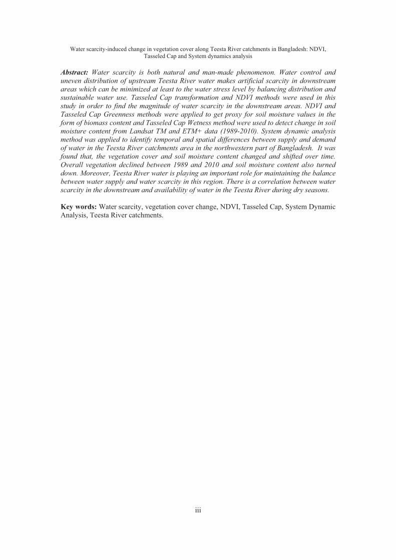
Abstract: Water scarcity is both natural and man-made phenomenon. Water control and uneven distribution of upstream Teesta River water makes artificial scarcity in downstream areas which can be minimized at least to the water stress level by balancing distribution and sustainable water use. Tasseled Cap transformation and NDVI methods were used in this study in order to find the magnitude of water scarcity in the downstream areas. NDVI and Tasseled Cap Greenness methods were applied to get proxy for soil moisture values in the form of biomass content and Tasseled Cap Wetness method were used to detect change in soil moisture content from Landsat TM and ETM+ data (1989-2010). System dynamic analysis method was applied to identify temporal and spatial differences between supply and demand of water in the Teesta River catchments area in the northwestern part of Bangladesh. It was found that, the vegetation cover and soil moisture content changed and shifted over time. Overall vegetation declined between 1989 and 2010 and soil moisture content also turned down. Moreover, Teesta River water is playing an important role for maintaining the balance between water supply and water scarcity in this region. There is a correlation between water scarcity in the downstream and availability of water in the Teesta River during dry seasons. Key words: Water scarcity, vegetation cover change, NDVI, Tasseled Cap, System Dynamic Analysis, Teesta River catchments.


Water scarcity-induced change in vegetation cover along Teesta River catchments in Bangladesh: NDVI, Tasseled Cap and System dynamics analysis
1
Introduction The quantitative revolution in geography has been fifty years and during this time
geography has reached enormous progress in building and implementing models of geographical systems (Batty, 2010). Due to technological development nowadays it becomes easy to examine various complex geographic problems. Within the last decade spatial dynamic modeling became possible for analysis of large-scale real-life ecosystems (Costanza & Voinov, 2004). The need to model spatial dynamics for geographic problems is becoming more obvious with the extensive use of spatial database handling, so called Geographic Information Systems (GIS). GIS has been used to quickly and reliably process spatially referenced data as a decision support tool and it provides the functions that allow a user to examine the spatial relationships among entities (Wang, 2004).
Water scarcity in a geographic region can identify (based on) the gap between demand and supply in a local circumstance. This demand of water includes both natural ecosystem and various human economics activities, that is per capital population pressure on the natural water supply and the percentage of natural water resources utilized to satisfy various human demands, including agriculture and different forms of irrigation, versus those contributing to ecological services and ecosystem functions (Dow, 2005). Therefore, water scarcity in a geographic region is not only a natural problem but also a human made phenomenon (UNDESA, 2005). Uneven water control in the upstream country makes artificial water scarcity in different part of the world. It is possible to minimize at list to the water stress level by balance distribution and sustainable uses.
This water control mainly happened because of the higher demand in a local
circumstance due to the growth in population, water needed in agriculture, energy and industry and partly because of climate change and contamination of water supplies (Mishra & Singh, 2011). This water scarcity in agriculture compounded by draught that has relation with available of surface water, and ground water resources.
To measure water scarcity or draught satellite data are useful and many indices are
used in GIS. Although, there is no single index that is used universally, many draught indices have been developed based on different perspectives. Recently developed drought measurement techniques relies on biophysical parameters including vegetation indices (VIs), land surface temperature (LST), soil moisture, albedo, and evapotranspiration (ET) (Chang et al., 2010). However, the early quantitative indices were developed based on climatic and meteorological observations Palmer Drought Severity Index (PDSI), and Standardized Precipitation index (SPI) for instance are remarkable in this context.
To determine impact assessment from drought, vegetation indexes are widely used to
evaluate draught condition as a proxy measurement. To calculate biomass changes over time Normalized Difference Vegetation Index (NDVI) is the most popular. Moreover, Vegetation Condition Index (VCI), Temperature Condition Index (TCI), the Soil-Adjusted Vegetation Index (SAVI) are also used for evaluate drought conditions indirectly. This study considers NDVI and Tasseled Cap analysis to measure vegetation cover change and water scarcity over 20 years in the Teesta catchments in Bangladesh. Moreover, System dynamic analysis also included in this study to evaluate present situation, measure trend of change over time and create future prediction by simulation modeling.
Md. Azizur Rahman
2
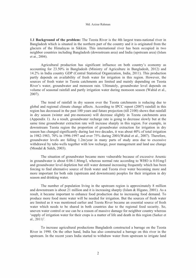
1.1 Background of the problem: The Teesta River is the 4th largest trans-national river in Bangladesh which is situated in the northern part of the country and it is originated from the glaciers of the Himalayas in Sikkim. This international river has been occupied in two neighbor countries including Bangladesh (downstream area) and India (upstream area) (Islam et at., 2004).
Agricultural production has significant influence on both country’s economy as accounting for 23.50% in Bangladesh (Ministry of Agriculture in Bangladesh, 2012) and 14.2% in India country GDP (Central Statistical Organization, India, 2011). This production partly depends on availability of fresh water for irrigation in this region. However, the sources of fresh water in Teesta catchments are limited and mainly depending on Teesta River’s water, groundwater and monsoon rain. Ultimately, groundwater level depends on volume of seasonal rainfall and partly irrigation water during monsoon season (Wahid et al., 2007).
The trend of rainfall in dry season over the Teesta catchments is reducing due to global and regional climate change affects. According to IPCC report (2007) rainfall in this region has decreased in the past 100 years and future projection (till 2100) shows that rainfall in dry season (winter and pre-monsoon) will decrease slightly in Teesta catchments area (Appendix 1). As a result, groundwater recharge rate is going to decrease slowly but at the same time groundwater extraction rate will increase sharply in this region. For example, in downstream Teesta region the proportion of groundwater extraction for irrigation in dry season has changed significantly during last two decades, it was about 40% of total irrigation in 1982-1983, 70% in 1996-1997 and over 75% during 2001(Wahid et al., 2007). Therefore, groundwater levels are falling 1.2m/year in many parts of study area due to excessive withdrawal by tube-wells together with low recharge, poor management and land use change (Mondal & Saleh, 2003).
The situation of groundwater became more vulnerable because of excessive Arsenic
in groundwater is about 0.06-1.86mg/l, whereas normal rate according to WHO is 0.01mg/l and groundwater level depletion but still water demand increasing frequently which has been forcing to find alternative source of fresh water and Teesta river water becoming more and more important for both side (upstream and downstream) peoples for their irrigation in dry season and drinking water.
The number of population living in the upstream region is approximately 8 million and downstream is about 21 million and it is increasing sharply (Islam & Higano, 2001). As a result, it became important to enhance food production due to increasing food demand. To produce more food more water will be needed for irrigation. But the sources of fresh water are limited as it was mentioned earlier and Teesta River became an essential source of fresh water which needs to be shared in both countries due to the regional food security. So, uneven water control or use can be a reason of massive damage for neighbor country whereas ‘supply of irrigation water for their crops is a matter of life and death in this region (Sarker et al., 2011)’.
To increase agricultural productions Bangladesh constructed a barrage on the Teesta River in 1990. On the other hand, India has also constructed a barrage on this river in the upstream. In the recent years India started to withdraw water from upstream to irrigate land

Water scarcity-induced change in vegetation cover along Teesta River catchments in Bangladesh: NDVI, Tasseled Cap and System dynamics analysis
3
and for industrial use; for that reason, very limited fresh water is available in downstream during dry season in the Teesta Barrage Project (TBP) area.
Under these circumstances it is critical to achieve food security and sustainable
livelihood in northern part of Bangladesh. In addition, water scarcity influencing regional change which is ultimately resulted in less food production, deforestation, arable land reduction and overall landscape change in that region. Consequently, environmental refuge is increasing sharply because famine situation already exists at some stage in dry season (from November to March) within downstream region.
This seasonal food crisis in downstream Teesta catchments called Monga. According
to Sebastian Zug (2006), ‘Monga is a seasonal food insecurity in ecologically vulnerable and economically weak parts of north-western Bangladesh, primarily caused by an employment and income deficit before aman is harvested. It mainly affects those rural poor, who have an undiversified income that is directly or indirectly based on agriculture’.
During Monga season many people move from this region to other region in the country. Dhaka (capital of Bangladesh) for instance, considers popular destination for those people and they move there to find their livelihoods. Thus, Dhaka city has been overloaded by huge population and many socio economic problems are increasing there rapidly. Currently more than 16 million people are living within approximately 1500sq. km area (Statistical Pocket Book, 2008).
Mainly, due to increase massive populations along the Teesta River, it makes tremendous pressure on limited natural resources in this region. Situation becomes complex due to lack of food security and further environmental degradation. To exaggerate food productions for the enormous demand the arable land has been harvested tremendously and people using extreme chemical fertilizer (mainly urea), extracting water from under the ground and river that is eventually a big warning for further environmental degradation for long terms perspective in this region.
However, to meet the demand of food, there is no alternative without intensive
agricultural practices. Thus, increasing food production, sharing fresh water become significant as short term solution but ultimately to come up with sustainable solution new innovations (hybrid foods, natural fertilizer), reduced chemical fertilizers use and sustainable use of limited natural resources are important.
For that reason, decision makers need to understand that how variables are interacting
with each other to create the situation. After having clear idea about interactive variables they also need to take initiatives to find sustainable solution for both short term and long term. Whereas the main problem began with shortage of water in dry season but still sources of water are limited, seasonal rainfall for instance are totally natural and it is out of control, in this situation, to manage existing situation it is essential to consented groundwater or available others fresh water sources.

Md. Azizur Rahman
4
1.2 Aim of the study: The ultimate goals of the study are:
a) To find water scarcity in downstream Teesta River and how the variables are interacting.
b) To find the vegetation cover change in the downstream Teesta catchments over 20 years.
c) To detect how water scarcity is correlated with vegetation cover change in the downstream Teesta catchments.
1.3 Overview of the study area: This study considers Teesta River catchments area in both West Bengal of India and Northern part of Bangladesh. Total catchments area in India about 8500 square km up to the barrage site (Majumdar, 1999) and 2750 square km in Bangladesh (Islam & Higano, 2001). However, according to Environmental Information System (ENVIS) centre Sikkim, total catchments area 10155 sq. km in India and 2004 sq. km in Bangladesh. Of the total area 8051 sq. km is covered by hilly region in the state of Sikkim and West Bengal in India and 4108 sq. km is plane land in West Bengal and Bangladesh (Table 1).
Table 1 Catchments Area of Teesta river (in sq. km)
Landscape State/region Sq. km Total (i) Sikkim 6930 Hilly Region (ii) West Bengal 1121
8051
(i) West Bengal 2104 In Plain (ii) North Bengal Bangladesh
2004 4108
Total in India : 10155 Total in Bangladesh : 2004
Total : 12159 Yet, current study will focus mainly northern part of Bangladesh (Figure 1). To
understand problem regarding water sharing (water available, demand and crisis) within two neighboring countries this study will consider two important irrigation projects (Table 2) based on Teesta River which are situated approximately 85km apart from each others.

Water scarcity-induced change in vegetation cover along Teesta River catchments in Bangladesh: NDVI, Tasseled Cap and System dynamics analysis
5
India
China
Burma
Thailand
Pakistan
Laos
Nepal
Bangladesh
Cambodia
Bhutan
Vietnam
Sri Lanka
100°0'0"E
100°0'0"E
90°0'0"E
90°0'0"E
80°0'0"E
80°0'0"E70°0'0"E
30°0'0"N 30°0'0"N
20°0'0"N 20°0'0"N
10°0'0"N 10°0'0"N
Dhaka
Rajshahi
Khulna
Sylhet
ChittagongBarisalBarisalBarisal
BarisalKhulna
Barisal
BarisalBarisal
Nilphamari
Rongpur
Lalmonirhat
Dinajpur
STUDY AREA MAP
STUDY AREABANGLADESH
�
60 0 60 120 180 24030Kilometers
Figure 1 Location map of the study area

Md. Azizur Rahman
6
In India (West Bengal) the Teesta barrage is situated at 26°45'13"N latitude and 88°35'21"E longitude at Gajoldoba point and in Bangladesh Teesta barrage situated at Dalia point 26°10'43"N latitude and 89° 3'6"E longitude. Both barrages are important for local irrigation project and for sustainable food production in their own region.
Table 2 Comparison between Gajoldoba & Dalia barrage and related irrigation projects
Comparison between two irrigation project
Gajoldoba (India) Dalia (Bangladesh)
Location 26°45'13"N latitude & 88°35'21"E longitude (WGS 84)
26°10'43"N latitude & 89° 3'6"E longitude(WGS 84)
Landscape Mixed (Hilly and plain land) Plain land
Climate Tropical; mild winter, hot, humid summer (March to June); humid,
warm rainy monsoon (June to October).
Tropical savanna and humid subtropical
Target area 922 000 ha 750 000 ha Irrigation potential 527 000 ha 540 000 ha Type of soil Sandy or clayey loam 80% alluvial Currently under irrigation
527 000 ha 111 000 ha
Power generation 67.50MW No Link cannels 210.79km 275km Beneficiaries 8 million people 21 million people
Although, climate in West Bengal India and Northern part of Bangladesh is similar, landscape are totally different. Combination of hilly and plane land in West Bengal is a barrier to practice intensive agriculture but in Bangladesh total Teesta catchments are plan lands that are very useful to harvest three times in a year.
Total target area for irrigation at Gajoldoba 922 000 ha and 750 000 ha at Dalia project. However, currently about 527 000ha in the upstream and only 111 000 ha in downstream are under irrigation due to the lack of water during dry season.
Both barrages included link cannels for water distribution over the irrigation project
area but only Gajoldoba project (India) has 67.50MW hydropower. Nevertheless, the big difference with the numbers of beneficiaries; in upstream it is including 8 million people and in downstream almost three times higher than upstream is about 21 million consequently (Islam & Higano, 2001). 1.3.1 Teesta River profile: Teesta is the forth main river in terms of discharge in Bangladesh (Reaz et al., 2010) which originates at an elevation of 5,280 m in the northeastern corner glaciers in Sikkim, India (State of Environment Sikkim (SES), 2007) and enters into Bangladesh at Chatnai, Nilphamari district. After traversing a length of about 414 km in India and Bangladesh it is meets with the second largest river name Jamuna in Bangladesh (Banglapedia, 2006) at an elevation of 23 m (SES, 2007). ‘It is a sandy braided river with steep slope, exhibiting high seasonal flow variability and cause inundation of floodplains in monsoon and low flow conditions in dry season’(Reaz et al., 2010). While passing through

Water scarcity-induced change in vegetation cover along Teesta River catchments in Bangladesh: NDVI, Tasseled Cap and System dynamics analysis
7
the Himalayan to the plains in West Bengal it is receives drainage from a number of tributaries on either side of its course which are listed in table 3 (SES, 2012). Table 3 Major Tributaries of Teesta River
Sl. No. Left-bank Tributaries Right-bank Tributaries 1. 2. 3. 4. 5.
Lachung Chhu Chakung Chhu Dik Chhu Rani Khola Rangpo Chhu
Zemu Chhu Rangyong Chhu Rangit River
In the mountain gorges, the width of the river Teesta is 30 to 40 m during autumn (SES, 2007). However, the average depth of this river varies 1.8 m and 4.5 m, respectively and from Chungthang to Singtam, the bed slope varies from approximately 35 m/ km to 17 m/ km. The velocity of this river in hilly region 6m/sec and in the plain it is about 2.4 to 3m/sec (SES, 2007).
Historically this river course has been shifted due to river erosion and some natural events. Up to the 18th century for example it flowed directly into the Padma River. However, due to excessive rainfall during 1787 a big flood event choked the original Atrai river channel. This resulted in the Teesta bursting into the Ghaghat which at that time was a very small river (Banglapedia, 2006). Many natural events including, land erosion, earthquakes, floods and geological structure changes have taken place in the northern part of the country and affected the original flows of the Karatoya, Atrai and Jamuneshwari rivers. The present Teesta is the result of these physical changes that accumulated flows of the Karaotoya, Atrai and Jamuneshwari rivers into the Teesta. The name Teesta actually came from the Bangle name Tri-Srota that means three flows together (Banglapedia, 2006).

Md. Azizur Rahman
8
Literature reviewThe current study examines water scarcity in the northern part of the Bangladesh and
uses satellite data. To reach the goal, NDVI, Tasseled Cap and system dynamic analysis is combined in this study. Therefore, this chapter provides short descriptions of the conceptual backgrounds. Moreover, brief descriptions of the review of literature in the study area and convenient techniques for water scarcity measurements from satellite data has also been illustrated in this chapter. 2.1 Water scarcity: Water scarcity is defined in relation water needs for livelihoods (Dow et al., 2005). These needs include daily needs for a person in his daily life and also for his livelihoods. According to Dow (2005), the indicator of water scarcity depends on water demand in very two specific purposes; for example, per capita population pressure on the natural water supply and the percentage of natural water resources utilized to satisfy various human demands, including agriculture and different forms of irrigation, versus those contributing to ecological services and ecosystem functions.
According to United Nation Department of Economics and Social affairs (UNDESA), ‘Water scarcity is both a natural and a human-made phenomenon. There is enough freshwater on the planet for six billion people but it is distributed unevenly and too much of it is wasted, polluted and unsustainably managed’. Therefore, in some region in the globe, water control and uneven distribution makes artificial scarcity which can be minimized at list to the water stress level by balance distribution and sustainable uses.
The terms water stress and water scarcity is not the same. ‘Water scarcity is defined as the point at which the aggregate impact of all users impinges on the supply or quality of water under prevailing institutional arrangements to the extent that the demand by all sectors, including the environment, cannot be satisfied fully’. On the other hand, ‘water stress define is an area ‘experiencing water when annual water supplies drop below 1700 m3 per person’. But when annual water supplies drop below 1000 m3 per person, the population faces water scarcity, and below 500 cubic metres absolute scarcity (UNDESA, 2005)’. 2.2 Water Scarcity and Bangladesh: Bangladesh is a country that is quite often portrait as climate vulnerable country in the world. It has long experiences of straggling with floods, tropical cyclone and sea level rise related hazards. Therefore, many national and international researchers considered Bangladesh as study area and tried to sketch her as water abandoned country (Rahman, 2005). This is obvious due to the temporal distribution of water resources; especially wet monsoon season during June to August is quite a lot rainfall over the country and upstream catchments in India (Mbugua & Snijders, 2011). This excessive water in the transnational rivers and heavy rainfall over the country are the main reasons for big floods which usually make big damages frequently in Bangladesh and it become international news. However, it does not reflect the real scenario in Bangladesh at all.
The water scarcity is a recent phenomenon in Bangladesh and it has direct relation
with the gap between demand and supply locally during dry season. Bangladesh in particular is heavily dependant on water due to the human consumption, irrigation, transportation and conservation of biodiversity (PRIO, 2012). Mainly, massive population growth, less than sufficient water flows in rivers, drawing down of ground water have made the region highly vulnerable to water stress.

Water scarcity-induced change in vegetation cover along Teesta River catchments in Bangladesh: NDVI, Tasseled Cap and System dynamics analysis
9
The temporal distribution of water resources is Bangladesh can be divided into two
extremes, one is wet season from June to October and another is the dry season between months December to May (Rahman, 2005). During dry season country become severely water stress especially northern part of the country because of the very low precipitation, high evaporation, very less water in transnational rivers. Day by day the situation is worsening because of the impact of climate change on weather patterns (PRIO, 2012).
The overall situation during dry season in the northern part of the country is becoming
crucial, due to the lack of regional food security. Paul (1998) noted ‘droughts are a recurrent phenomenon in Bangladesh, afflicting the country at least as frequently as major floods and cyclones’. Moreover, he mentioned it has attracted far less scientific attention than floods or cyclones. Habiba (2012) mentioned Bangladesh may experience 5-6% increase of rainfall by 2030 due to glacier melting and more intense monsoon which will create frequent, big and prolonged floods as well as increased droughts outside the monsoon season. Therefore, it is a big challenge nowadays for Bangladesh to find a sustainable solution for regional food security and natural disaster. 2.3 Land use and land cover change: Land Use and Land Cover Change (LULCC) is a general term for the human modification of Earth's terrestrial surface. Though humans have been modifying land to obtain food and other essentials for thousands of years, current rates, extents and intensities of LULCC are far greater than ever in history, driving unprecedented changes in ecosystems and environmental processes at local, regional and global scales (The Encyclopedia of Earth, 2011).
According to USGS website ‘Land use and land cover change is a pervasive environmental phenomenon that modifies land cover characteristics and affects a broad range of socio-economic, biologic, geologic, and hydrologic systems and processes’. They suggest that to understand the impact of land use and land cover change and their associated feedbacks on environmental systems it is need to understand of their rates, patterns, and drivers of past, present, and future land use change. Nowadays, Land use and land cover changes are of concern to a wide variety of stakeholders, scientists, and citizens due to the impacts on economic health and sustainability, practices of land management and social and political process. 2.4 Relation between water scarcity and land use and land cover change: Water scarcity has a strong correlation with land use in natural ecosystem process. However, potential land use and land management practices have impact on the need to protect the quantity and quality of water resources, while water availability is a pre-requisite for land uses requiring irrigation (Weatherhead & Howden, 2009). Furthermore, Maeda et al., (2010) addressed the link between water resource and land use and they have mentioned both are closely linked to each other and with regional climate, assembling a very complex system. For agricultural and economic development water is a key resource and scarcity of water can hamper both processes. Therefore, Water security requires a balance between water gain and loss (Guo-yu et al., 2012).
Md. Azizur Rahman
10
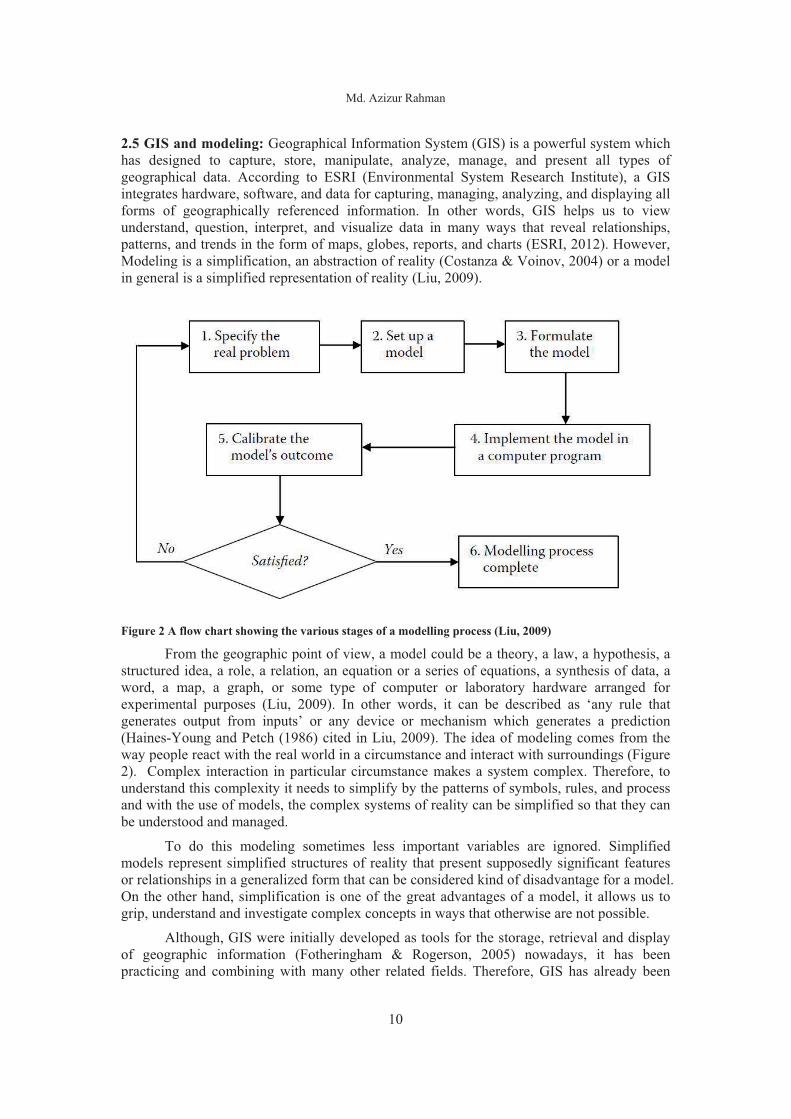
2.5 GIS and modeling: Geographical Information System (GIS) is a powerful system which has designed to capture, store, manipulate, analyze, manage, and present all types of geographical data. According to ESRI (Environmental System Research Institute), a GIS integrates hardware, software, and data for capturing, managing, analyzing, and displaying all forms of geographically referenced information. In other words, GIS helps us to view understand, question, interpret, and visualize data in many ways that reveal relationships, patterns, and trends in the form of maps, globes, reports, and charts (ESRI, 2012). However, Modeling is a simplification, an abstraction of reality (Costanza & Voinov, 2004) or a model in general is a simplified representation of reality (Liu, 2009).
Figure 2 A flow chart showing the various stages of a modelling process (Liu, 2009)
From the geographic point of view, a model could be a theory, a law, a hypothesis, a structured idea, a role, a relation, an equation or a series of equations, a synthesis of data, a word, a map, a graph, or some type of computer or laboratory hardware arranged for experimental purposes (Liu, 2009). In other words, it can be described as ‘any rule that generates output from inputs’ or any device or mechanism which generates a prediction (Haines-Young and Petch (1986) cited in Liu, 2009). The idea of modeling comes from the way people react with the real world in a circumstance and interact with surroundings (Figure 2). Complex interaction in particular circumstance makes a system complex. Therefore, to understand this complexity it needs to simplify by the patterns of symbols, rules, and process and with the use of models, the complex systems of reality can be simplified so that they can be understood and managed.
To do this modeling sometimes less important variables are ignored. Simplified models represent simplified structures of reality that present supposedly significant features or relationships in a generalized form that can be considered kind of disadvantage for a model. On the other hand, simplification is one of the great advantages of a model, it allows us to grip, understand and investigate complex concepts in ways that otherwise are not possible.
Although, GIS were initially developed as tools for the storage, retrieval and display of geographic information (Fotheringham & Rogerson, 2005) nowadays, it has been practicing and combining with many other related fields. Therefore, GIS has already been

Water scarcity-induced change in vegetation cover along Teesta River catchments in Bangladesh: NDVI, Tasseled Cap and System dynamics analysis
11
expands its boundary and as a result of the development of powerful hardware and updated software it has now come up in a contemporary platform and integrated with many others spatial analysis and modeling system. The main strength of GIS for Spatial analysis and modeling were discussed in Goodchild and Longley (2005) and it has summarized by Maguire et al., 2005 in their book ‘GIS, Spatial analysis, and modeling’ within four specific categories are follows:
Data management: GIS provide an environment in which to manage and model massive input and output data sets, as well as temporary data sets created during analyses they can also manage metadata about model parameters. More than this, a GIS can be a source of data for analysis and modeling. The versioning capabilities of GIS can also be used to handle design alternatives or model scenarios. Data integration/transformation: Today's GIS usually offer an extensive collection of tools for loading, reformatting, transforming, and integrating data. This could be as simple as reprojecting several files to a common map projection or could involve many steps to transform data into a common database structure; GIS are also adept at bringing together disparate data and workers operating in different disciplines. Visualization/mapping: GIS have excellent mapping capabilities. They are especially strong at static 2D and 3D mapping and visualization. Some Systems can display 3D scenes and moving objects in near real time, and some also offer basic ESDA facilities. Spatial analysis and modeling capabilities: In recent years, basic GIS software systems have been extended with an ever-more-sophisticated range of spatial analysis and modeling options. The strength of GIS provides opportunity to Integration of GIS, simulation models and computer visualization. It has already implemented in various planning practices in the field of geography. Surface and subsurface water models for instance use GIS to address resource and environmental issues (Cowen et al. (1995), Darbar, et al. (1995), Merchant (1994) Smith & Vidmar (1994), Tim & Jolly (1994), Warwick & Haness (1994) cited in Wang, 2004). Moreover, some others type of models includes simulations for example the interactions between land use and transport to connect economic activities in space with accessibility as well as the demand and supply for flows (Barra, 2001, cited in Wang, 2004) can also be mentioned.
In an integrated system of GIS, simulation modeling and computer visualization, gives opportunity to contribute each distinctive feature of a system to examine complex problem and can be a reliable decision support tools by feedback simulation modeling. However, GIS provides the functions that allow a user to examine the spatial relationships among entities (Wang, 2004). On the other hand, Simulation models are capable to calculate dynamic relationship over time in a complex interrelated feedback effect and the strength of visualization can represent data in a way that may reveal patterns and relationships that are hard to detect using non-visual approaches such as text and tables (Wang, 2004).
Spatial and temporal resolution determines the relationship between the real world and the model of the real world that is constructed in the computer (Maguire, et al., 2005). Analysis of temporal and spatial resolution change is possible when GIS and simulation models are integrated.

Md. Azizur Rahman
12
2.6 System dynamics and GIS: Combination of System Dynamic (SD) analysis and Geographical Information System (GIS) is a new approach called Spatial System Dynamics (SSD) which can present the model of feedback based dynamic processes in time and space. This new approach has grounded in control theory for dispersed constraint system (Ahmad & Simonovis, 2004). It is capable to offer a single modeling framework for calibrate conceptually different models particularly combine spatial and non-spatial interaction among model feedbacks based complex process in time and space (Figure 3). Therefore, it is able to examine different types of physical and natural processes in spatial and temporal variety.
As a result it became a reliable approach to examine many common complex dynamic
system including environmental process, climate change, natural hazard management, land use and land cover changes, water and natural resource management.
Change in land cover for instance, caused by conversion or is the most substantial human induced alternation of the Earth System (Le et al., 2010). To understand the process of human land use consequence it is important to observe scientific experimentations, derived through careful observations and feedbacks (Le et al., 2010). In this process GIS based observation can be used as significant tools for temporal resolution changes. However, complex interaction among variables requires feedback analysis in dynamics process because the dynamics of the coupled human environment system are inherently complex and uncertain in time and space. Therefore, alternatively, a scenario-based approach (System Dynamics) has been recognized as a natural and useful way for advancing the problem of viewing the system's future in the face of high complexity and uncertainty (Le et al., 2010). As a result combination of GIS and System Dynamics approach can be considered as sustainable solution for these types of problems.
However, the capabilities of GIS are rooted in static map-based analysis and their considerable success at managing natural and physical resources as assets (Batty (2005), cited in Maguire et.al., 2005). Yet, to manage fuzzy, uncertain, and dynamic, and to be successful at characterizing and simulating real-world processes, GIS must be able to incorporate multidimensional space-time modeling (Maguire et al., 2005). It can be considered as limitations of present GIS software. Therefore, it is necessary to hire in non-geographic
Figure 3 Architecture of spatial system dynamics approach (Ahmad S. & Simonovis S.P, 2004)

Water scarcity-induced change in vegetation cover along Teesta River catchments in Bangladesh: NDVI, Tasseled Cap and System dynamics analysis
13
modeling and simulation software systems, for instance, GoldSim and STELLA. This non-geographic simulation software can be considered as graphical icon-based modeling tools that represent the structure of a module diagramatically, and are comparatively easy to handle in general (Robert Voinov & Alexey (Eds), 2004). 2.7 Convenient techniques of draught /water scarcity measurements: Water scarcity has been frequently increasing nowadays in many part of the world due the growth in population and expansion of agricultural, energy and industrial sectors, and partly because of climate change and contamination of water supplies (Bates et al., 2008 and Mishra & Singh, 2011). The water scarcity is again compounded by droughts (Mishra & Singh, 2011) and it has direct relation with surface water and ground water resources which can lead to reduced water supply, deteriorated water quality, crop failure and disturbed riparian habitats (Riebsame et al., 1991, cited in Mishra and Singh, 2011 ).
To identify draught a number of indicators for drought monitoring and assessment are used (Murad & Islam, 2011). Because of the complexity of drought, there are no single index has been able to adequately capture the intensity and severity of drought and its potential impacts (Petros et al., 2011). Therefore, indicators has been developed based on different perspectives, for example recently developed drought measurement techniques rely on biophysical parameters including vegetation indices (VIs), land surface temperature (LST), soil moisture, albedo, and evapotranspiration (ET) (Chang et al., 2010). However, the early quantitative indices were developed based on climatic and meteorological observations.
To measure draught impact, vegetation indices are commonly used that express drought conditions indirectly (Chang, et.al., 2010). Normalized Difference Vegetation Index (NDVI), Vegetation Condition Index (VCI), Temperature Condition Index (TCI), the Soil-Adjusted Vegetation Index (SAVI), Enhanced Vegetation Index (EVI), are some of the well known and extensively used vegetation indices (Hasan et al., 2011).
From the metrological point of view, the best known drought index worldwide is the
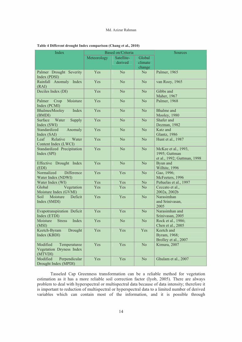
Palmer Drought Severity Index (PDSI) (Palmer (1965) cited in Petros et al., 2011), while other famous indices are the Standardized Precipitation index (SPI). Based on meteorology, Satellite-derived and Global climate change most popular indices are listed in the table 4.
Md. Azizur Rahman
14
Table 4 Different drought Index comparison (Chang et al., 2010)
Based on/Criteria Index Meteorology Satellite-
derived Global climate change
Sources
Palmer Drought Severity Index (PDSI)
Yes No No Palmer, 1965
Rainfall Anomaly Index (RAI)
Yes No No van Rooy, 1965
Deciles Index (DI) Yes No No Gibbs and Maher, 1967
Palmer Crop Moisture Index (PCMI)
Yes No No Palmer, 1968
BhalmeeMooley Index (BMDI)
Yes No No Bhalme and Mooley, 1980
Surface Water Supply Index (SWI)
Yes No No Shafer and Dezman, 1982
Standardized Anomaly Index (SAI)
Yes No No Katz and Glantz, 1986
Leaf Relative Water Content Index (LWCI)
Yes No No Hunt et al., 1987
Standardized Precipitation Index (SPI)
Yes No No McKee et al., 1993, 1995; Guttman et al., 1992; Guttman, 1998
Effective Drought Index (EDI)
Yes No No Byun and Wilhite, 1996
Normalized Difference Water Index (NDWI)
Yes Yes No Gao, 1996; McFeeters, 1996
Water Index (WI) Yes Yes No Peñuelas et al., 1997 Global Vegetation Moisture Index (GVMI)
Yes Yes No Ceccato et al., 2002a, 2002b
Soil Moisture Deficit Index (SMDI)
Yes Yes No Narasimhan and Srinivasan, 2005
Evapotranspiration Deficit Index (ETDI)
Yes Yes No Narasimhan and Srinivasan, 2005
Moisture Stress Index (MSI)
Yes No No Rock et al., 1986; Chen et al., 2005
Keetch-Byram Drought Index (KBDI)
Yes Yes Yes Keetch and Byram, 1968; Brolley et al., 2007
Modified Temperaturee Vegetation Dryness Index (MTVDI)
Yes Yes No Kimura, 2007
Modified Perpendicular Drought Index (MPDI)
Yes Yes No Ghulam et al., 2007
Tasseled Cap Greenness transformation can be a reliable method for vegetation
estimation as it has a more reliable soil correction factor (Iyob, 2005). There are always problem to deal with hyperspectral or multispectral data because of data intensity; therefore it is important to reduction of multispectral or hyperspectral data to a limited number of derived variables which can contain most of the information, and it is possible through
Water scarcity-induced change in vegetation cover along Teesta River catchments in Bangladesh: NDVI, Tasseled Cap and System dynamics analysis
15
transformations such as, Tasseled Cap (Kauth & Thomas, 1976) or Principal Component Analysis (PCA). 2.8 Previous studies in the study area: This study examines water scarcity based on satellite data and investigates a case in the Teesta river catchments in the Bangladesh. This area is known as crops grain area of Bangladesh because the soils of this region are fertile. The biggest national irrigation project Teesta Barrage Project (TBP) is situated here. Recently, impact of climate change (low precipitation, high evaporation), excessive water withdrawal in upstream, low water flows in Teesta River, ground water depletion and excessive arsenic in ground water, makes situation vulnerable in this region. Therefore, few studies have taken place from different perspectives in this study area.
Murad et al. (2011) used MODIS data for investigate agricultural and metrological draught in the northern part of Bangladesh and they used Standardized Precipitation Index (SPI) and NDVI to examine their case. To identified draught affected area in Bangladesh Paul (1998) has recognized draught effected household by questioner survey and examine the means by which residents of a drought-affected area of Bangladesh cope with this hazard. The farmer’s perception and awareness, impacts and adaptation measures of farmers towards drought has assessed by Habiba et al. (2012). Rahman (2005) discussed water problems in Bangladesh and the consequence of floods and draughts from the socio-economical and environmental development point of view.
Hanif (1995) conducted a detailed study about hydro-geomorphic characteristics
including water discharge, course shifting pattern, water level, duration of floods, sediment characteristics and ground water conditions in this region. A brief history of India-Bangladesh barrage establishment and water sharing during 1955-1983 can be found in Abbas (1984) ‘the Ganges Water Dispute books’. Discharge based economic valuation of irrigation water in Teesta river has taken place in Mullick, et al. (2011) study. They tried to develop the total and marginal benefit functions of the key off-stream water use, irrigation, as a function of flow in the Teesta River of Bangladesh. From the hydrological perspective Mullick et al. (2010) analyzes the flow characteristic of the Teesta River in Bangladesh and they used 40 years historic flow data and further estimate the environmental flow requirements for the River.
Islam & Higano (2001) propose optimal utilization of Teesta water and tried to find out a sustainable solution by their statistical analysis. Moreover, they have also investigated environment and socio economic effects on Teesta River catchments. Ground water was estimated and limits of ground water can be used were identified based on the recharge characteristics and interactions between groundwater use for irrigation and land use change by Wahid et al. (2007). Due to the establishment of Teesta barrage how the local climate has been reflected investigated by Sarker et al. (2011). They find out the change of climatic parameters including temperature, precipitation, humidity, evaporation and so on. Zug (2006) focus seasonal food crisis in the catchments area and defined Monga as seasonal food crisis in his study.

Md. Azizur Rahman
16
Methods and material This chapter includes data collection for both satellite data and ancillary data from
different sources and methods used for satellite image processing for this study.
3.1 Methodical Overview: The study has completed in the few steps are following:
� Data collection o Satellite data o Secondary data
� Literature studies � Data analysis
o Normalized Difference Vegetation Index (NDVI) o Tasseled Cap o System modeling and integration with vegetation cover change data
� Reporting 3.1.1 Data collection: To collect satellite data few criteria have considered including data availability, cloud coverage, seasonality, expected temporal resolution (5years interval) and so on. The availability of data in the study area has started from 1989 TM band but data from 1990 to 1999 was not available. However, from 2000-2012 mostly ETM+ band and few are TM (2005, 2010) were available. After 2004 ETM+ data has some problem due to sensor error (although it has included gap mask) and most of the data has excessive cloud coverage. According do research objectives, dry season is most important period to compare within temporal resolution. Therefore, it has also taken place under consideration to determine useful data.
Secondary data related to upstream and downstream catchments; including meteorological data, population and its growth rate, detail about Teesta barrage in West Bengal (Gajoldoba) and Teesta barrage in Bangladesh (Dalia), Teesta barrage Irrigation projects; total target area for both irrigation projects, under irrigated areas, number of industries, ground water availability, recharge rate and extraction, water demand in various sectors, water demand change in near future, water supply, landscape in both catchments, type of soils, floods event during study period and so many other relevant data has collected from published research papers, various government and non-governmental responsible organizations annual reports and also from their websites.
3.1.2 Literature studies: Literatures have chosen according to the ground of the current study. To understand the terms that is used in this study has described and few definitions have also been included in this part. Moreover, this part also provides short descriptions of the relevant conceptual backgrounds, convenient techniques for water scarcity measurements from satellite data and so on. Finally, it has end up with the background of the water scarcity in Bangladesh and available research has found in the study area. 3.1.3 Data analysis methods: Landsat satellite data, administrative vector data and ancillary data has used in the analysis part. To analyzed satellite data Normalized Difference Vegetation Index (NDVI) and Tasseled Cap transformation methods are considered for vegetation cover change detection. System dynamics analysis has performed based on
Water scarcity-induced change in vegetation cover along Teesta River catchments in Bangladesh: NDVI, Tasseled Cap and System dynamics analysis
17
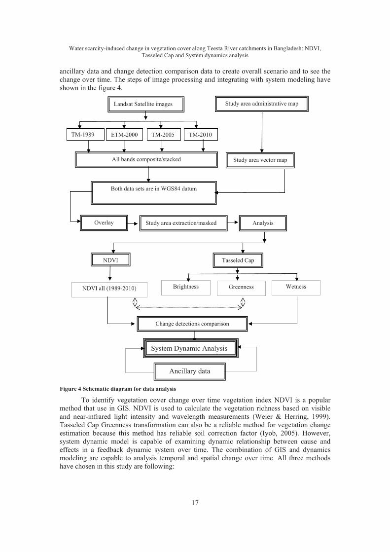
ancillary data and change detection comparison data to create overall scenario and to see the change over time. The steps of image processing and integrating with system modeling have shown in the figure 4. Figure 4 Schematic diagram for data analysis
To identify vegetation cover change over time vegetation index NDVI is a popular method that use in GIS. NDVI is used to calculate the vegetation richness based on visible and near-infrared light intensity and wavelength measurements (Weier & Herring, 1999). Tasseled Cap Greenness transformation can also be a reliable method for vegetation change estimation because this method has reliable soil correction factor (Iyob, 2005). However, system dynamic model is capable of examining dynamic relationship between cause and effects in a feedback dynamic system over time. The combination of GIS and dynamics modeling are capable to analysis temporal and spatial change over time. All three methods have chosen in this study are following:
Both data sets are in WGS84 datum
Overlay Study area extraction/masked
Change detections comparison
Landsat Satellite images
All bands composite/stacked
Study area administrative map
TM-1989
Study area vector map
ETM-2000 TM-2005 TM-2010
Analysis
NDVI Tasseled Cap
NDVI all (1989-2010) Brightness Greenness Wetness
System Dynamic Analysis
Ancillary data

Md. Azizur Rahman
18
3.1.4 Normalized Difference Vegetation Index (NDVI): The vegetation index NDVI has been used for many years to measure and monitor plant growth (vigor), vegetation cover, and biomass from multispectral satellite data (USGS, 2010). The mechanism of this method depends on the reflection of both wavelengths, visible and near-infrared from the plants leaves (Rahman, 2010) and it is calculate the reflectance data in the both (near-infrared and visible red parts) of the electromagnetic spectrum.
The following equation is utilized for obtaining NDVI: NDVI = (NIR - RED) / (NIR + RED)
NIR is near-infrared radiation (0.7 �m to 1.1 �m respectively) which is reflected by
healthy vegetation. However, the color of plant leaf and its chlorophyll strongly absorbs visible wavelength more specifically, red band (0.4 �m to 0.7 �m) because this wavelength is used in photosynthesis. So the mechanism is green vegetation or the healthy vegetation absorbs most of the visible light (Red band) that come on it, and reflects a large portion of the near-infrared light. Therefore, less vegetation or low biomass reflects less near-infrared radiation (Weier & Herring, 1999).
How much wavelength should be affected depends on the number of leaves the plants
have. Researchers can measure the intensity of light coming off the Earth in visible and near-infrared wavelengths and quantify the photosynthetic capacity of the vegetation in a given pixel of land surface (Rahman, 2010). If visible wavelength is poorly reflected then near-infrared wavelengths mean the vegetation in that pixel is likely to be dense and may contain some type of forest. However, if the variations of intensity of both wavelengths reflected are not adequate then the vegetation is probably sparse and may consist of grassland, tundra, or desert (Rahman, 2010).
As a result, Pixels with higher NDVI value characterized with high proportion of green biomass, whereas low NDVI value indicate low green biomass, while absence of vegetation on the surface, for instance water or bare soil do not show response, and stressed vegetation exhibit decline in NDVI magnitude (Liu, 2003). According to this definition Weier & Herring (1999) characterize NDVI value for a given pixel and they mentioned NDVI values is always follow certain scale of measurement that has a specific range from minus one (-1) to plus one (+1). Maximum value in this scale close to +1 (0.8 - 0.9) indicate the highest possible density of green leaves or biomass and close to zero (0) point to the no green vegetation. Moreover, values below 0.1 correspond to barren areas of rock, sand, or snow; higher values from 0.2 to 0.3 indicate shrub and grassland; and temperate and tropical rainforests normally presents by values ‘between’ 0.6 to 0.8.
3.1.5 Tasseled Cap: Tasseled Cap transformation is a commonly used transform that can be used for reducing spectral information from multiple bands into a single measure of interest to the user (Toomey, 2011). In this transformation, it is possible to manipulation of the band Brightness values using coefficients that Kauth and Thomas estimated in the late 1970s. Therefore, this transformation is also known as Kauth-Thomas transformation or KT Transformation.
Tasseled Cap transformation is one of the available transformation methods for enhancing spectral information content of Landsat MSS, TM and ETM data. According to the ENVI user’s guide, for the Landsat MSS data, this transformation normally performs an
Water scarcity-induced change in vegetation cover along Teesta River catchments in Bangladesh: NDVI, Tasseled Cap and System dynamics analysis
19
orthogonal transformation for the source data to a new four-dimensional space as well as the soil Brightness index (SBI), the green vegetation index (GVI), the yellow stuff index (YVI), and a non-such index (NSI) associated with atmospheric effects.
Same transformation for the Landsat TM data, the Tasseled Cap consists of three factors: Brightness, Greenness, and Third. The Brightness and Greenness are equivalent to the MSS Tasseled Cap SBI and GVI indices and the third component is related to soil features, including moisture status.
However, for the Landsat 7 ETM data this transformation create 6 different bands
including Brightness, Greenness, Wetness, Fourth (Haze), Fifth, Sixth. But first three bands contain maximum features; therefore these first three are more important than others. In this case first measure is overall Brightness, or albedo of a pixel which is called Brightness. The second is the Greenness and is similar to NDVI and designed to indicate the degree of vegetation cover. The third is Wetness which is designed to indicate moisture content of the surface (Toomey, 2011).
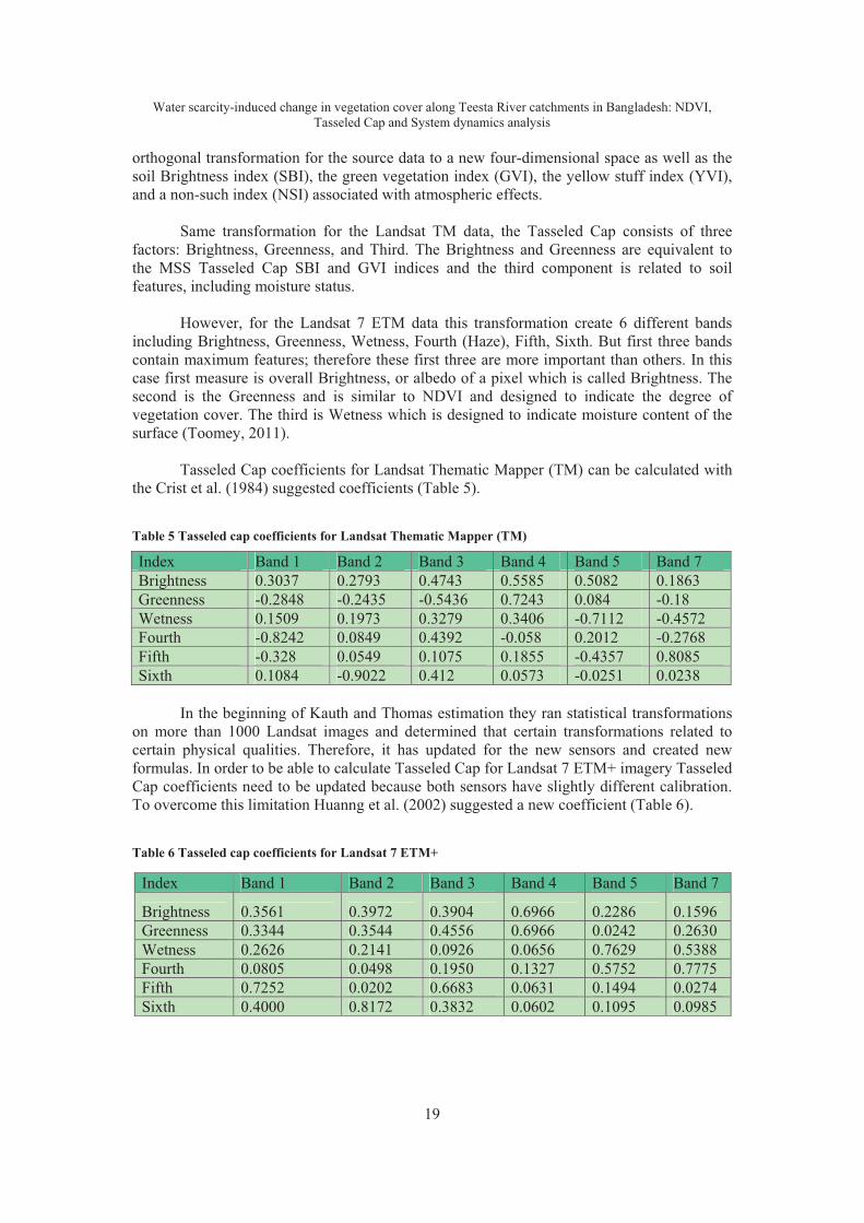
Tasseled Cap coefficients for Landsat Thematic Mapper (TM) can be calculated with the Crist et al. (1984) suggested coefficients (Table 5).
Table 5 Tasseled cap coefficients for Landsat Thematic Mapper (TM)
Index Band 1 Band 2 Band 3 Band 4 Band 5 Band 7 Brightness 0.3037 0.2793 0.4743 0.5585 0.5082 0.1863 Greenness -0.2848 -0.2435 -0.5436 0.7243 0.084 -0.18 Wetness 0.1509 0.1973 0.3279 0.3406 -0.7112 -0.4572 Fourth -0.8242 0.0849 0.4392 -0.058 0.2012 -0.2768 Fifth -0.328 0.0549 0.1075 0.1855 -0.4357 0.8085 Sixth 0.1084 -0.9022 0.412 0.0573 -0.0251 0.0238
In the beginning of Kauth and Thomas estimation they ran statistical transformations
on more than 1000 Landsat images and determined that certain transformations related to certain physical qualities. Therefore, it has updated for the new sensors and created new formulas. In order to be able to calculate Tasseled Cap for Landsat 7 ETM+ imagery Tasseled Cap coefficients need to be updated because both sensors have slightly different calibration. To overcome this limitation Huanng et al. (2002) suggested a new coefficient (Table 6).
Table 6 Tasseled cap coefficients for Landsat 7 ETM+
�
Index Band 1 Band 2 Band 3 Band 4 Band 5 Band 7
Brightness 0.3561 0.3972 0.3904 0.6966 0.2286 0.1596 Greenness 0.3344 0.3544 0.4556 0.6966 0.0242 0.2630 Wetness 0.2626 0.2141 0.0926 0.0656 0.7629 0.5388 Fourth 0.0805 0.0498 0.1950 0.1327 0.5752 0.7775 Fifth 0.7252 0.0202 0.6683 0.0631 0.1494 0.0274 Sixth 0.4000 0.8172 0.3832 0.0602 0.1095 0.0985

Md. Azizur Rahman
20
Overall, Tasseled Cap transformation highlights the characteristics of vegetation, and soil (Zhang, 2009), as a result urbanized areas are particularly distinct in the Brightness components, but in the greater biomass covering, the best brighter pixel can be found in Greenness image. On the other hand, Wetness layer provides subtle information about the moisture status of the wetland environment (Zhang, 2009). 3.1.6 System modeling and integration with vegetation cover change data: ‘System dynamics refers to the re-creation of the understanding of a system and its feedbacks’ (Haraldsson, 2004). The aim of the system dynamics are explore dynamic responses in a given system to changes within or from outside the system over time. The term system dynamics was first discussed in the sixties by Jay Forester at MIT (Forester, 1961 and Haraldsson, 2004). According to MIT System Dynamics in Education Project (MDEF), ‘System dynamics is an approach to understand the behaviour of complex systems over time. It deals with internal feedback loops and time delays that affect the behaviour of the entire system’. Generally, a design or a mental model describe the past and predict the future and system dynamics deal with the same model by mathematical representation which can be consider secondary steps of mental model that widely deals with and numerical analysis and understanding of uncertainty of the practical representation in the developed mathematical model (Haraldsson, 2004). Nowadays, it is connected with building computer models of complex problem situations and then experimenting with and studying the behaviuor of these models over time (Caulfield & Maj, 2001).
System modeling has included in this study to examining dynamic relationship among inter-related variables in a feedback dynamic system over time. The system model is created based on a Causal Loop Diagram (CLD) and it is presents in result section (Figure 12). ‘A CLD is a simple map of a system with all its constituent components and their interactions’ (Donella, 2008). A causal loop diagram revel the structure of a system by capturing interaction and consequently the feedback loops among variables. Therefore, the function of CLD’s is to map out the structure and the feedbacks of a system in order to understand its feedback mechanisms (Haraldsson, 2004).
The case for this study consist transnational river water distribution issue between
Bangladesh and India and water scarcity in the downstream region. As a result, to examine dynamic relationship between variables and to find out gap between supply and demand of water the system has included all variables for the sources of water coming into the system, demand and uses in the existing situation for both upstream and downstream. 3.1.7 Reporting: The report is include the background and the aim of the study, methods and materials that have been used in this dissertation, related literatures, results, discussion, limitation and summary of the study.
3.2 Materials: Landsat TM and ETM+ satellite images from 1989 to 2010 used for Normalized Difference Vegetation Index (NDVI) and Tasseled Cap analysis. Detail about Landsat satellite data, including name of the satellite, type of sensor, number of bands and acquisition date is include in the table 5. The administrative vector maps has used as a reference map for extracting study area from digital images. Local Government Engineering and Development (LGED) administrative map used as a reference map for site selection. Detail ancillary data about study area, climate and irrigation projects has collected from various secondary sources for use in system modeling and comparative discussion.

Water scarcity-induced change in vegetation cover along Teesta River catchments in Bangladesh: NDVI, Tasseled Cap and System dynamics analysis
21
Table 7 Satellite data used in the current study
Space craft Sensor Number of bands Acquisition date Landsat 4 TM 7 19 January 1989 Landsat 7 ETM+ 8 19 February 2000 Landsat 5 TM 7 07 January 2005 Landsat 5 TM 7 06 February 2010
Individual band specification for the Landsat TM and ETM+ sensors is presents table 6 and table 7 accordingly. Landsat TM data are sensed in seven spectral bands simultaneously. However, out of seven bands, band number sex senses thermal (heat) infrared radiation. As a result, Landsat TM can only acquire night scenes in band 6. Moreover, Landsat TM scene has an Instantaneous Field Of View (IFOV) of 30m x 30m in all bands except band no 6, while band 6 has an IFOV of 120m x 120m on the ground (NASA, 2012).
Table 8 Band specification for TM
Band Number μm Resolution 1 0.45-0.52 30 m 2 0.52-0.60 30 m 3 0.63-0.69 30 m 4 0.76-0.90 30 m 5 1.55-1.75 30 m 6 10.4-12.5 120 m 7 2.08-2.35 30 m
Table 7 includes band specification for ETM+ sensor. This sensor has eight-band, multispectral scanning radiometer which is capable of providing high-resolution imaging information of the Earth's surface. The new features in Landsat 7 are a panchromatic band with 15 m spatial resolution, an on-board full aperture solar calibrator, 5% absolute radiometric calibration and a thermal IR channel with a four-fold improvement in spatial resolution over TM (NASA, 2012). Table 9 Band specification for ETM+
Band Number μm Resolution 1 0.45-0.515 30 m 2 0.525-0.605 30 m 3 0.63-0.69 30 m 4 0.75-0.90 30 m 5 1.55-1.75 30 m 6 10.4-12.5 60 m 7 2.09-2.35 30 m 8 0.52-0.9 15 m

Md. Azizur Rahman
22
According to NASA, An ETM+ scene has an Instantaneous Field Of View (IFOV) of 30 meters x 30 meters in bands 1-5 and 7 while band 6 has an IFOV of 60 meters x 60 meters on the ground and the band 8 an IFOV of 15 meters.

Water scarcity-induced change in vegetation cover along Teesta River catchments in Bangladesh: NDVI, Tasseled Cap and System dynamics analysis
23
ResultsSpatial investigation is possible to interpret the systems and processes of natural and
socio-economic changes by interpreting satellite imageries and incorporating many additional data which is causing the changes on earth’s surface. When looking at water scarcity or drought, the application of NDVI indicator for instance, is used to evaluate how vegetation cover is changing over time and compared to the metrological data (Tucker & Choudhury (1987), Fensholt & Rasmussen (2011), Hein et al., 2011). Soil moisture and NDVI can also be combined to identify water scarcity in a geographic region. Therefore, in this study NDVI and Tasseled Cap methods were used to identify vegetation cover change over time. Moreover, GIS techniques can handle efficiently both spatial and statistical analyses of the acquired data. GIS techniques made it easy and possible to show spatial extent, magnitude and change over time through spatial visualization techniques.
4.1 Results for NDVI change: The vegetation cover has been changed over time. Analysis of NDVI from different maps reveals that, the density of the vegetation has decreased over the study period ‘between’ year 1989 to year 2010 (Figure 5). Maps are presents linear stretch between the values defined by the standard deviation.
In 1989 the NDVI map represents the highest density of vegetation over the study
area while vegetation map for 2000 showed that the value of NDVI has increased in the south-eastern edge and somewhat in the middle of the study area otherwise it was found as low in the study area. However, the NDVI comparison graph represents both highest and lowest NDVI were found in the year 2000 although, mean NDVI value showed no changes for this year (Figure 6).
Figure 5 NDVI comparison between 1989-2010
NDVI MAP (1989-2010)NDVI 1989
10 0 10 20 30 405Kilometers
LegendNDVIValue
High : 1
Low : -1
NDVI 2000
NDVI 2010NDVI 2005
Ì

Md. Azizur Rahman
24
NDVI Comparison
-0.6
-0.4
-0.2
0
0.2
0.4
0.6
0.8
1989 2000 2005 2010
Min
Max
Mean
St. dv
Pixel values with high standard deviation correspond to intensive vegetation cover, while pixel values with lower standard deviation corresponds to the areas with sparse vegetation (Abbasova, 2010). According to standard deviation distribution in the graph (Figure 6) it can be assumed that, the overall vegetation coverage has partially increased from 1989 to 2000. In 2005 minimum value of NDVI has increased a little but highest values of NDVI dropped below 0.4 whereas mean value has not been changed significantly. Standard deviation has also decreased to some extent.
Overall green vegetation coverage decreased in 2005. From 2005 to 2010 NDVI
values has not changed significantly. South-eastern part of the study area became greener than any other parts of the study area. Although top left and bottom left parts became less green. However, statistically from 2005 to 2010 overall change is not that much remarkable. Mainly, during this time period vegetation distribution has been changed from one part to another. Change in vegetation cover in 2010 has showed a centralized pattern in some specific parts of the study area.
To visualize results from NDVI analysis, initially a definition by Weirer and Herring,
(1999) was followed (Appendix 11). However, it was found almost impossible to draw a boundary with the given value range. To overcome this difficulty a new reclassification method were adopted considering the natural breaks from the histogram analysis and reclassified NDVI images into six different classes (Table 8). All new classes were assigned new class name according to assumption and experience by the author. The same class (with the same data ranges) was applied for all data sets. The results from new classification are presented in figure 7.
Table 10 Land cover classification relatively to NDVI values
Class no NDVI value range Land cover 1 <-0.05 Water 2 -0.05 � -0.031 Barren land 3 -0.031 � 0.01 Open land 4 0.01 � 0.11 Crop land 5 0.11 � 0.17 Green vegetation 6 >0.17 Dense vegetation
From the reclassification results, most of the study area was found as crop land.
Approximately 50% total study area was identified as this land use class. It was obvious that
Figure 6 NDVI statistics comparison ‘between’ 1989-2010

Water scarcity-induced change in vegetation cover along Teesta River catchments in Bangladesh: NDVI, Tasseled Cap and System dynamics analysis
25
the area should have covered by the crops because of the biggest irrigation project Teesta Barrage Project (TBP) is situated within this study area boundary.
The proportion of green vegetation and open land looks nearly similar and both of the land uses has been taken account about 20%. But the dense vegetation and water bodies covered a smaller portion of the study area which is roughly less than 7% (Figure 8). However, barren land has been found as lowest portion and it was about 2% of the total land uses. So, the highest land class in this area was found as crops land and the lowest land class was found barren land.
The distribution of land use classes has been scattered over the study area except water bodies and barren land. Water bodies found mainly in Teesta River and along with barren lands which is situated along the course of this River.
Open land and crops land has been distributed over the study area. Nonetheless,
Green vegetation and dense vegetation was found shifted in different places. The major land class crop land has been changed over time.
The figure (Figure 8) shows that in 1989 and 2005 has similar portion (about 55%) of crop land over the study area but in 2005 it was only 25 approximately, although in 2010 it has increased 45%. This change appeared due to temporal resolution in satellite images and seasonality in crops growing. Image in 1989 and 2005 was taken in January 19 and January 07 respectively. On the other hand, image from 2000 and 2010 was taken in February 19 and February 06 correspondingly. As a result, it can be assumed that crops in field appeared in both 1989 and 2005 images.
Figure 7 Land cover classification relatively to NDVI values and changes over time
NDVI RECLASS MAP (1989-2010)
LegendWater
Barren Land
Open Land
Crops Land
Green vegetation
Dense vegetation
NDVI Reclass 2010
10 0 10 20 30 405Kilometers
NDVI Reclass 2005
NDVI Reclass 1989 NDVI Reclass 2000
Ì

Md. Azizur Rahman
26
Open land and green vegetation has maintain a sequence over the study period. It has not included any significant quantitative change from year to year but the distribution pattern has been changed. The distribution of green vegetation in the year 1989, 2005 and 2000, 2010 looks similar respectively. Although, dense vegetation was distributed over study area in 1989 and 2005 but it has been centralized in the south-eastern part during 2000 and 2010.
Overall NDVI result showed that vegetation biomass decreased over time during study period. However, from 1989 to 2000 vegetation biomass partly increased otherwise it was decreased. Summary of results does not reflect enormous changed. Vegetation was shifter from one place to another place during study period. As result, NDVI statistics does not show big change but vegetation were declined most of the places in study area whereas some part of the study area become greener at the same time.
4.2 Tasseled Cap analysis results: Tasseled Cap transformation for TM data consists of three factors these are: Brightness, Greenness, and Wetness. Nevertheless, ETM+ data consists of six different bands which are: Brightness, Greenness, Wetness, Haze, Fifth, Sixth. For both cases these first three components are important and contain maximum information. This study has been included three TM (1989, 2005 and 2010) and one (2000) ETM+ data sets for the analysis. The results from this analysis are presented in the figure 9.
For the Tasseled Cap analysis first measure is called Brightness, or albedo of a pixel. The second is the Greenness and it is similar to NDVI and designed to indicate the degree of vegetation cover (which has been compared later on in this study). The third one is Wetness which is designed to indicate moisture content of the surface (Toomey, 2011). In this study it has been designed to measure vegetation cover change over time due to water scarcity, change in soil moisture content (Wetness) and change in Greenness indices to measure water scarcity in the study area.
Results from Tasseled Cap analysis are presented overall change between 1989 and
2010 (Figure 9). The change in three above mentioned components were represented together in composite map in the mentioned figure. From Tasseled Cap analysis it was found converse features of Brightness and Greenness. Barren land, urbanized area or open land was distinct in the Brightness components, on the other hand, dense biomass coverage were represented by Greenness components and moist features were represented by Wetness components.
0%
20%
40%
60%
80%
100%
1989 2000 2005 2010
Landuse changes over time
Water Barren Land Open Land Crops Land Green vegetation Dense vegetation
Figure 8 Land cover classes relatively to NDVI value change over time

Water scarcity-induced change in vegetation cover along Teesta River catchments in Bangladesh: NDVI, Tasseled Cap and System dynamics analysis
27
To represents the features the mechanism of Brightness is presented here with a
weighted sum of all six bands found from the data sets that is a measure of overall reflectance by differentiating light from dark soils. Although, Greenness representing contrast between near-infrared and visible reflectance, as a result it represents density of green vegetation. The third component of the composite maps represents contrast between shortwave-infrared (SWIR) and visible/ near-infrared (VNIR) reflectance that is a good indicator of soil moisture content.
From the composite maps it can be illustrated that Brightness were found mainly along the Teesta River over the study period and slightly spread over the study area that has been changed ‘between’ 1989 and 2010. At the same time, for Greenness component, 1989 image looks greener than other temporal resolution. Overall, Greenness and Brightness has been changed and shifted. Year between 1989, 2005 and 2000, 2010 looks similar for both Greenness and Brightness. For the year 1989 and 2005 heights Greenness found in the top right parts (Figure 9) and lowest Greenness found in the bottom left edge but Wetness centralized in the bottom right side. Similarly, 2000 and 2010 Tasseled Cap components have been changed following similar patterns. In this case, dense green areas were found in the south-eastern part and wet areas were found in the south-western edges. However, Brightness centralized along Teesta River between year 2000 and 2010. Figure 9 Tasseled cap composite map and change over time
TASSELED CAP CHANGE OVER TIME (1989-2010)
TASSELED CAP 2000
TASSELED CAP 2005 TASSELED CAP 2010
10 0 10 20 30 405Kilometers
LegendTasseled Cap
Brightness
Greenness
Wetness
ÌTASSELED CAP 1989

Md. Azizur Rahman
28
To compare statistics
for Greenness and Wetness both components has been separated from composite band to single band by ASCII-raster transformation and results are presents through maps and graphs. The Wetness change over time map can be found in the appendix (Appendix 3) and statistical comparison presents in the figure 10.
The figure 10 shows that Wetness has been changed over time. Pixels with high standard deviation values correspond to the high Wetness in the surface or indicate higher moisture content of the surface. On the other hand, low standard deviation values correspond to the surface with low moisture content. According to this definition, moisture content into the surface has been increased from 1989 to 2000. Nonetheless, after year 2000 Wetness has been decreased over the study periods. The similar changing pattern has been found in mean values. Although, highest and lowest value distribution shows different patterns, in 1989 for example the highest value was approximately 120 but it has been increased 150 to 170 between 2000 and 2005. The minimum value for the Wetness components was not that much fluctuated within temporal resolutions.
Results from Greenness component’s band change over time presents in appendix
(Appendix 2). The results show that vegetation has declined over time during study period. The Greenness algorithm has been calibrated to the calculation contrast between near-infrared and visible reflectance, therefore it is able to calculate density of green vegetation. The higher pixels value represents more possibility of green vegetation and lower Greenness value connected to less possibility of green biomass.
The Greenness components from Tasseled Cap and vegetation index NDVI is capable
to reveal similar results. As a result Greenness component can be used for validate NDVI results. Results (Pixel value) from both methods were compared and it has found that pixel with high NDVI also given upper Greenness values. Thus, results from Greenness component and NDVI have compared and presents in a single map (Figure 11). Although both classifications contain different scale of measurements, so it was generalized by histogram stress function instead of reclassification for both results.
Wetness comparison
-300-250-200-150-100-50
050
100150200250
1989 2000 2005 2010
Min
, max
-80
-60
-40
-20
0
20
40
60
Mea
n st
.dv
Min Max Mean St. dv
Figure 10 Wetness comparisons ‘between’ 1989-2010

Water scarcity-induced change in vegetation cover along Teesta River catchments in Bangladesh: NDVI, Tasseled Cap and System dynamics analysis
29
TASSELED CAP GREENNESS AND NDVI COMPARISON NDVI 1989
NDVI 2010GREENNESS 2010
GREENNESS 1989
Ì
Legend GreennessNDVI
High : 18.8167
Low : -129.905
High : 1
Low : -1
10 0 10 20 30 405Kilometers
To compare and visualize results from both methods it was defines a histogram stretch (that can be applied to the rasters to enhance their appearance) so called linear stretch between the percent clip minimum and percent clip maximum. The majority of the pixel values fall within an upper and lower limit. Therefore, it was reasonable to trim off the extreme values.
To compare NDVI
and Tasseled Cap Greenness, 1989 and 2010 images were chosen. The result of vegetation cover change patterns looks quite similar for both selected years between 1989 and 2010. Higher green vegetation over the study area was found in 1989 and lower vegetation was found in the year 2010. Both methods identified that, the green vegetation has been reduced and the spatial distribution of vegetation coverage changed during the study period.
Figure 11 Comparison between NDVI and Tasseled cap greenness component

Md. Azizur Rahman
30
4.3 System dynamic analysis result: Before going to the detail results it is important to illuminate the process of system building and the boundary of the system. To examine dynamic relationship among inter-related variables and the impact on vegetation cover change due to water scarcity over time in downstream the study used STELLA simulation models based on a conceptual model called Causal Loop Diagram (CLD) (Figure 12). The model was created based on background problem in the study area.
The limited sources of water supply along Teesta River, huge demand of water for both upstream and downstream and gap between demand and supply were considered in the modeling process.
The CLD shows that water availability in upstream depends on natural glacial molting
in Shikim Himalayan, rainfall and ground water. Moreover, water release to the downstream is also important variables to determinate how much water is available in upstream. However, downstream water availability relies on rainfall, ground water and water release in upstream Teesta River. Water have been using in both catchments according to their demand.
Water demand in both catchments is similar and it has been using mainly by agriculture, forestry, industries, and household activities. However, the amount of water that is required for both catchments depends on the availability of arable land in agriculture, non crop vegetation (forest), number and type of industries and the population living in the catchments.
Population growth in both catchments relies on food availability and net migration.
Population migration is directly related to the economic growth rate in this region but economic growth rate depends on industry and agricultural products. On the other hand, population growth is considered as the reason for arable land reduction that is connected to less agricultural production.
Water satisfaction level in upstream and downstream depends on the balance between
water demand and supply for both catchments. If water supply is not enough according to the demands in both catchments then conflict risk increases (Figure 12).
Based on the Teesta river water control in upstream, availability of water in
downstream and water demand for both catchments the system has been divided into three separated parts including, upstream, downstream and Teesta River system. Upstream and downstream system created based on local demand and supply accordingly. Teesta River system integrated sources of water come in to the system and take out from the system according to the demand in both side but it has been included a subsystem is called Brahmaputra River system because a certain amount of water has restricted (20%) to go to the destination river system (Appendix 7).

Wat
er sc
arci
ty-in
duce
d ch
ange
in v
eget
atio
n co
ver a
long
Tee
sta
Riv
er c
atch
men
ts in
Ban
glad
esh:
ND
VI,
Tass
eled
Cap
and
Sys
tem
dyn
amic
s ana
lysi
s
31
R
ainf
all
Tota
l pop
ulat
ion
inD
owns
tream
Gro
und
wat
er in
Dow
nstre
am
Food
ava
ilabl
e in
Dow
nstre
am-
+
Dow
nstre
amA
gric
ultu
re
Wat
er a
vaila
ble
inD
owns
trea
mTe
esta
Riv
er
Gla
cial
mol
ting
inSh
ikim
,H
imal
ayan
Tota
l Wat
er u
sein
Ups
trea
m
+To
tal p
opul
atio
n in
Ups
tream
Tota
l wat
er d
eman
din
Ups
trea
m
-+
Wat
er d
eman
dA
gric
ultu
re in
Ups
tream
Wat
er d
eman
dIn
dust
ry in
Ups
tream
+
+
Tota
l wat
er u
se in
dow
nstr
eam
Wat
er d
eman
d in
Indu
stry
In D
owns
tream
Wat
er d
eman
din
Agr
icul
ture
inD
owns
tream
+
-+
Wat
er d
eman
d in
Dow
nstr
eam+
+
Con
flict
risk
Wat
er s
atisf
actio
nle
vel i
n U
pstre
am
--
+
Glo
bal w
arm
ing +
-
Wat
er a
vaila
ble
inU
pstr
eam
Tee
sta
Riv
er
+G
roun
d w
ater
inup
stre
am+
+
+
-
+
+
-
Net
mig
ratio
nU
pstr
eamU
pstre
am A
gric
ultu
re
Food
ava
ilabl
ein
Ups
tream
-
Tota
l ind
ustry
inD
owns
tream
Tota
l ind
ustry
inU
pstre
am
+
+
Tota
l Ara
ble
land
inD
owns
tream
Tota
l Ara
ble
land
inU
pwns
tream
-
+
-
Econ
omic
gro
th ra
tein
Dow
nstre
amEc
onom
ic g
roth
rate
in U
pstre
am
+
+
+
+
Net
mig
ratio
nD
owns
tream +
+
++
R
+
B
+
+
+
+
+
Agr
icul
tura
l Int
ensit
yD
owns
tream
+ -
+
+
Agr
icul
tura
lIn
tens
ity U
pstre
am
+
-
-
+
++
-
--
Wat
er S
atisf
actio
nle
vel i
n D
owns
tream
+
Nee
d fo
r so
lutio
n
+
Thin
k ab
out
poss
ible
sol
utio
n
Polit
ical
nego
tiatio
nJo
int w
ater
man
agem
ent s
yste
m
+
++
--
Non
cro
p ve
geta
tion
cove
rin
dow
nstre
am
+
+
-
+
+
+
+
+
+
+
-
+
+
Fi
gure
12
Cau
sal L
oop
Dia
gram
(CLD
) for
the
stud
y
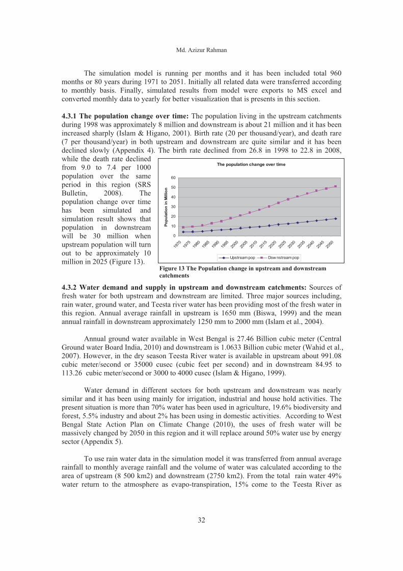
Md. Azizur Rahman
32
The simulation model is running per months and it has been included total 960 months or 80 years during 1971 to 2051. Initially all related data were transferred according to monthly basis. Finally, simulated results from model were exports to MS excel and converted monthly data to yearly for better visualization that is presents in this section. 4.3.1 The population change over time: The population living in the upstream catchments during 1998 was approximately 8 million and downstream is about 21 million and it has been increased sharply (Islam & Higano, 2001). Birth rate (20 per thousand/year), and death rare (7 per thousand/year) in both upstream and downstream are quite similar and it has been declined slowly (Appendix 4). The birth rate declined from 26.8 in 1998 to 22.8 in 2008, while the death rate declined from 9.0 to 7.4 per 1000 population over the same period in this region (SRS Bulletin, 2008). The population change over time has been simulated and simulation result shows that population in downstream will be 30 million when upstream population will turn out to be approximately 10 million in 2025 (Figure 13).
4.3.2 Water demand and supply in upstream and downstream catchments: Sources of fresh water for both upstream and downstream are limited. Three major sources including, rain water, ground water, and Teesta river water has been providing most of the fresh water in this region. Annual average rainfall in upstream is 1650 mm (Biswa, 1999) and the mean annual rainfall in downstream approximately 1250 mm to 2000 mm (Islam et al., 2004). Annual ground water available in West Bengal is 27.46 Billion cubic meter (Central Ground water Board India, 2010) and downstream is 1.0633 Billion cubic meter (Wahid et al., 2007). However, in the dry season Teesta River water is available in upstream about 991.08 cubic meter/second or 35000 cusec (cubic feet per second) and in downstream 84.95 to 113.26 cubic meter/second or 3000 to 4000 cusec (Islam & Higano, 1999). Water demand in different sectors for both upstream and downstream was nearly similar and it has been using mainly for irrigation, industrial and house hold activities. The present situation is more than 70% water has been used in agriculture, 19.6% biodiversity and forest, 5.5% industry and about 2% has been using in domestic activities. According to West Bengal State Action Plan on Climate Change (2010), the uses of fresh water will be massively changed by 2050 in this region and it will replace around 50% water use by energy sector (Appendix 5). To use rain water data in the simulation model it was transferred from annual average rainfall to monthly average rainfall and the volume of water was calculated according to the area of upstream (8 500 km2) and downstream (2750 km2). From the total rain water 49% water return to the atmosphere as evapo-transpiration, 15% come to the Teesta River as
Figure 13 The Population change in upstream and downstream catchments
The population change over time
0
10
20
30
40
50
60
1970
1975
1980
1985
1990
1995
2000
2005
2010
2015
2020
2025
2030
2035
2040
2045
2050
Popu
latio
n in
Mill
ion
Upstream pop Dow nstream pop
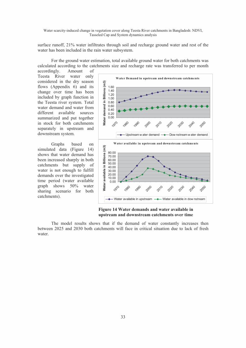
Water scarcity-induced change in vegetation cover along Teesta River catchments in Bangladesh: NDVI, Tasseled Cap and System dynamics analysis
33
surface runoff, 21% water infiltrates through soil and recharge ground water and rest of the water has been included in the rain water subsystem. For the ground water estimation, total available ground water for both catchments was calculated according to the catchments size and recharge rate was transferred to per month accordingly. Amount of Teesta River water only considered in the dry season flows (Appendix 6) and its change over time has been included by graph function in the Teesta river system. Total water demand and water from different available sources summarized and put together in stock for both catchments separately in upstream and downstream system. Graphs based on simulated data (Figure 14) shows that water demand has been increased sharply in both catchments but supply of water is not enough to fulfill demands over the investigated time period (water available graph shows 50% water sharing scenario for both catchments).
The model results shows that if the demand of water constantly increases then
between 2025 and 2030 both catchments will face in critical situation due to lack of fresh water.
Figure 14 Water demands and water available in upstream and downstream catchments over time
Water Demand in upstream and downstream catchments
0.000.200.400.600.801.001.201.401.60
1970
1980
1990
2000
2010
2020
2030
2040
2050W
ater
dem
and
in B
illio
ns (m
3)
Upstream w ater demand Dow nstream w ater demand
Water available in upstream and downstream catchments
0.0010.0020.0030.0040.0050.0060.0070.0080.00
1970
1980
1990
2000
2010
2020
2030
2040
2050W
ater
ava
ilabl
e in
Bill
ions
(m3)
Water available in upstream Water available in dow nstream

Md. Azizur Rahman
34
4.3.3 Teesta River water sharing and impact on both catchments: Teesta River water system began with natural water flows coming into the system and rain water for both upstream and downstream has been considered for the sources of water in this system. Nonetheless, water release from the system is depends on upstream and downstream water outtake limits. In the upstream there is no limit to outtake water but it has been controlled by a percent calculator. On the other hand, downstream water outtake was restricted by 20% available flows release to the destination river (Brahmaputra River) but the amount of water in downstream Teesta is depends on how much water is coming into the downstream system form upstream channels. Based on water outtake proportion in upstream and impact of water availability in both upstream and downstream catchments few scenarios were created (Figure 15).
Figure 15 Availability of water in downstream related to the Teesta River water outtake proportion in upstream The graphs (Figure 15) were made from simulated data and it demonstrates that how important is Teesta River water in both catchments in trims of accomplishing the local demand for the agriculture, industry, forest (non crop vegetation) and domestic water uses. Water is a primary component for vegetation growth. As a result, it can be assumed that vegetation cover in both catchments is directly related to water availability in this region. According to the model results, if upstream outtake 45% of total water from the Teesta and release rest of the water to the downstream, then downstream region can sustain for long period for next 100 years without any problem but it can immediately made problem for upstream water supply. Conversely, if upstream takes 60% of total water from Teesta then it can survive for long period without any problem but downstream will be in big trouble within next 5 to 10 years. This critical situation has been created due to limited fresh water resources in this region and 50% outtake in upstream shows best scenario within the comparison. The graphs (Figure 15) shows that less than 50% Teesta River water available in downstream can be created a vulnerable situation and it may cause a significant environmental degradation in the study area.
Water outtake proportion in upstream and water available both catchments
0.00
20.00
40.00
60.00
80.00
100.00
120.00
140.00
1970 1975 1980 1985 1990 1995 2000 2005 2010 2015 2020 2025 2030 2035 2040 2045 2050
Billi
ons
(m3)
Water available in upstream(45%)
Water available indownstream(45%)
Water available in upstream(50% scenario)
Water available indownstream(50% scenario)
Water available in upstream(55% scenario)
Water available indownstream(55% scenario)
Water available in upstream(60% scenario)
Water available indownstream(60% scenario)

Water scarcity-induced change in vegetation cover along Teesta River catchments in Bangladesh: NDVI, Tasseled Cap and System dynamics analysis
35
Discussion
In this study, primarily an attempt was made to detect vegetation cover changes due to water scarcity in the downstream Teesta River catchments. The study was carried out on the basis of NDVI and Tasseled Cap analysis techniques. In order to get a proxy data set for soil moisture values in the form of biomass content Tasseled Cap Wetness were used. On the other hand NDVI were used to detect change in vegetation by detecting change in Greenness indices from satellite imageries. To predict water scarcity, evidence from satellite data analysis (NDVI and Tasseled Cap) and gap between demand and supply of Teesta river catchments were analyzed.
The demands for water in both upstream and downstream areas were calculated
considering both natural and socio-economic requirements. Per capita population pressure on the natural water supply has been considered at first place. Secondly, percentage of utilized natural water resources for satisfying various human demands including agriculture, household, industry versus those contributing to ecological services and ecosystem functions were taken into account. Therefore, system dynamic analysis was performed to identify interrelation among responsible variables for vegetation cover change over time due to water scarcity.
Both, NDVI and Tasseled Cap transformation methods has identified that the vegetation cover and soil moisture content has been changed over time. Overall vegetation declined between 1989 and 2010 and soil moisture also has turned down. However, the distribution pattern of soil moisture and vegetation biomass content showed a shifting tendency over the study area. For that reason in this study it was tried to find the answers of two important questions ‘where? And why?’ these changes had been occurred. An attempt was made to find out the areas with Spatial and temporal changes. In the section below the findings regarding changes in Spatial and Temporal patterns are described. 5.1 Spatial changes of vegetation: To find out spatial change within the investigated area, the study has been considered three possible criteria are as follows:
� According to Teesta Baarrage Project (TBP) boundary � Between farmland and natural harvesting area � Following type of soil
5.1.1 Vegetation cover changes inside and outside TBP: TBP has been completed successfully in August 1990 and operation commenced in 1993 (Islam & Higano, 2001). However, barrage in upstream (Gazoldoba) was started operation after two years TBP started serving the downstream areas. Therefore, the assumption was that, both irrigation projects (up and downstream projects) has partial relationship to increase or decrease vegetation within the project boundary.

Md. Azizur Rahman
36
Initially, TBP in downstream might help to increase vegetation within the proximity
of boundary but after opening upstream project, availability of water in downstream decreased drastically and TBP was facing difficulties to achieve goal and not helping anymore to grow more vegetation. An attempt was made to compare statistics between inside and outside TBP (Figure 16) to observe if there was any relationship between the water share of inside and outside of TBP boundary. From the statistics graph no significant changes were found during study period. The limitation of available data in expected temporal resolution (data missing between 1990 and 1999) and seasonality (crops season) might hampered to figure out the change in relation with inside and outside TBP boundary.
5.1.2 Vegetation cover changes between farmland and natural harvesting area: To investigate spatial change between farmland and naturally harvested areas identification of samples were done by choosing training areas from the investigated area (Appendix 8). Six different samples has been identified over the study area and compared with farmland and naturally harvested areas (Figure 17). Farmland was identified inside TBP project boundary and natural harvested areas were selected outside of the TBP territory. The comparison result showed that, vegetation biomass has been increased little bit in naturally harvested area than farmland over the study period. Moreover, vegetation biomass has been shifted and fluctuated from 1989 to 2010. Lowest biomass found in 1989 and 2005 but it was increased during 2000 and 2010.
Overall, the result shows that there are no big spatial changes between farmland and natural harvested sample area NDVI statistics except little fluctuations within temporal resolution. For both samples statistics has been changed following the similar trends.
Figure 16 NDVI comparisons between inside and outside TBP
Figure 17 Comparisons between farmland and natural harvested samples area
-0.5-0.4-0.3-0.2-0.1
00.10.20.30.40.50.6
1989 2000 2005 2010
NDVI comparison between TBP in & out sides.
Min(in) Min(Out) Max (in) Max(Out) Mean(in) Mean(out) Std(in) Std(Out)
-0.4-0.3-0.2-0.1
00.10.20.30.40.50.6
1989 2000 2005 2010
NDVI comparison between sample Farmland and Natural harvested area
Min(Far) Min(Nat) Max (Far) Max(Nat) Mean(Far) Mean(Nat) Std(Far) Std(Nat)

Water scarcity-induced change in vegetation cover along Teesta River catchments in Bangladesh: NDVI, Tasseled Cap and System dynamics analysis
37
5.1.3 Vegetation cover changes following type of the soil: Only five different types of soil were found in the study area. These are a) Barind tract soil; b) Grey floodplain and non-calcareous soil; c) Grey floodplain soil; d) Plain Terrace and mixed grey soil and e) Dark gray and brown floodplain soil. Both national soil map of Bangladesh (Banglapedia, 2006) and FAO high resolution digital soil map of the World (FAO, 2007) have been compared to identify soil types of the study area (Appendix 9). More than 85% of the study area has been surrounded by grey floodplain and non calcareous soil and most of the deforestation occurred in this area. However, except grey floodplain and non-calcareous soils area others soil type area either no change found or vegetation slightly increased. However, grey floodplain soil area becomes greener than other type of soils.
5.2 Temporal changes of vegetation: Vegetation of the study area has been changed over time and it can be related to many interrelated variables. Primarily this study has been considered to correlate few important variables are follows:
� Meteorological data including monthly average rainfall and temperature � Flood events during study period � Rapid Population Growth in the study area � Water availability in Teesta River
5.2.1 Vegetation cover changes due to rainfall and temperature changes: Climate variables rainfall and temperature has great importance to vegetation dynamics at both global and regional scales (Zeng & Yang, 2008). Higher temperature in tropical region is considered to be responsible for excessive evapotranspiration and it reduces effective soil moisture. The soil moisture is directly related to the vegetation growth; as a result temperature increase has negative impact on vegetation growth in the study area. On the other hand, rainfall has positive impact on vegetation growth. During monsoon season (July-August) in the study area the vegetation growth rate is higher than any other season due to heavy rain fall during this season. The monthly average rainfall and temperature (Figure 18) patterns have not changed a lot during the study period. As a result, meteorological data can not be correlated to the responsible variables for vegetation cover change in the study area. Figure 18 Monthly average rainfall and temperature
0100200300400500600700800900
Monthly Average rainfall (mm)
1988-89 1999-00 2004-05 2009-10
Monthly average temperature (°C)
05
101520253035
July Aug Sept Oct Nov Dec Jan Feb Mar Apr May June
1988-89 1999-00 2004-05 2009-10

Md. Azizur Rahman
38
5.2.2 Vegetation cover changes due to Floods events during study period: Flood in Bangladesh is a common phenomenon and the country has been suffering more or less almost every year. However, it is also important event for the natural replenishing groundwater levels, to fertilize fields by depositing fine sediments and to kill pests (Braun & Abheuer, 2011). Therefore, floods helps to increase agriculture production by increasing soil moisture content and increasing soil fertility which results increase in vegetation biomass.
However, excessive flooding can cause damage to crops, livestocks, infrastructure, and vegetation that creates huge social and economic hazards. More than 20% of the land surface inundated by flood water has been considered as big flood. The most memorable incidents of severe flooding in the recent pasts has been noted by Braun and Abheuer (2011), and they mentioned it occurred in 1988 and 1998 when 61% and 68%, of the country were submerged respectively (Figure 19) .
Figure 19 Maximum flooded area in Bangladesh from 1954 to 2008 (BWDB, 2008)
Moreover, medium size (more than 20% inundation of land) floods came into regular intervals and during study period it was occurred regularly. A big flood in recent past was in 1998 and the impact of this flood have been found in the soil moisture contain in 2000 image. Tasseled Cap Wetness analysis results showed that during 2000 Wetness index were increased (Figure 10). Moreover, NDVI and Tasseled Cap Greenness analysis showed that, vegetation cover also increased in some extent (Figure 5 & Appendix 2) during same time period. 5.2.3 Vegetation Cover Change due to Rapid Population Growth: Population pressure on land resource has been increased over time. The population has increased in upstream and downstream and future change prediction has been calculated by using simulation model and it was presented in figure 13 under the result section. The number of population was 21 million in 2008 in downstream and assumption was made from model simulation that is the number will increase more than 30 million during 2025 when upstream population will turn out to be 10 million approximately and number of people will reach 50 million by 2050 in downstream. Due to Rapid population growth during study period new settlements has been constructed that has impact on vegetation change over the study area. As a result, it can be assumed that reduction in the amount of arable land and vegetation degradation were the results from new settlements expansion.

Water scarcity-induced change in vegetation cover along Teesta River catchments in Bangladesh: NDVI, Tasseled Cap and System dynamics analysis
39
5.2.4 Water availability in Teesta River and vegetation cover changes: Water is a primary component for growing vegetation. Consequently, scarcity of water is strongly correlated to the reduction of vegetation and it can destroy the ecosystem and its underlying processes. Agricultural and economic growth in a region would be affected due to deforestation process. Thus, scarcity of water requires balance between water gain and loss (Guo-yu et al., 2012). The process of water scarcity in the study area directly related to the differences between demand and supply in local circumstance during dry seasons. Mainly, rapid growth of population, climate change impact (very low precipitation, high evaporation), lower water flows in rivers, drawing excessive ground water have made this region highly vulnerable to water stress. Sources of fresh water in the study area are limited throughout dry season and Teesta River water play an important role to keep balance among water supply for irrigation, biodiversity process, and socio-economic activities. Therefore, availability of water in the river directly connected to biodiversity process within the study area boundary. The dynamic analysis model has been simulated over the study period and it was found that the availability of less than 50% Teesta River water in downstream can create a vulnerable situation (Figure 15) due to deforestation, lack of water in agriculture, industry and human economic activities that may cause a significant environmental degradation in this region.

Md. Azizur Rahman
40
Limitation
It was difficult to find appropriate set of satellite data for this study due to lack of time series availability and accessibility (cost) of satellite imegeries. Possible data for this investigation was considered according to the literature studies (Table 9). Finally, Landsat TM and ETM+ data were selected as it was found free of cost and available image tiles from archives matches with the study area. However, it was not frequently available according to the expected temporal resolution. Some tiles were found as missing tiles in year between 1990 and 1999. Which may impact the result and it was critical to compare changes during this time period. Table 11 Overview of satellites/sensors useful for monitoring water scarcity
Satellites/sensor systems Resolution Used in following articles AVHRR 1000m Kogan, 1995. Tucker et al, 2005.
MODIS 250m Hasan et.al, 2011. Tucker et al, 2005. Jackson, et.al 2004
SMOS 50km Merlin, et.al 2012 SPOT 1.5 m, 6 m Boegh, et.al, 1999. Tucker et al,
2005Landsat 4 and 5 TM 30 m Mas, 1999. Boegh, et.al, 1999
Ancillary data related to the Teesta River water flows, water demand and supply for catchments area, population, industry, agriculture and arable land for both upstream and downstream was collected from various published papers and it was found a bit puzzling information. Published papers for both catchments might a little bit bias as it is still a big political issue between Bangladesh and neighboring India.
Landsat satellite data is required radiometrically and atmospheric corrected. Before it can be used to calculate Tasseled Cap or vegetation indices further transformation is needed. In order to be able to calculate Tasseled Cap, digital number (DN, 0-255) data must be converted to radiance, a physical measurement (Grant and Lane, 2011) and it was described by Huang et al. (2002). Huang used Landsat 7 ETM+ data and calculated Tasseled Cap coefficient which is only applicable for Landsat 7 ETM+ data but to be able to use in Landsat 5 TM data using a further transformation described in Vogelmann et al. (2001) because the two sensors have slightly different calibration. The study used both TM and ETM+ data but it was not included all transformation according to Vogelmann et al. However, 0 values were calculated as no data.
The results might have been influenced due to the lack of further transformation. Consequently, year 2000 image may have some impact due to different sensor calibration as it used only ETM+ data and rest of all was TM.
Tasseled Cap transformation can be used to identify cultivated vegetation
characteristics. Crist et al. (1986) sketched the spectral paths followed by a typical cultivated crop over the growing cycle (Appendix 10). Mainly TM Tasseled Cap data has been calculate

Water scarcity-induced change in vegetation cover along Teesta River catchments in Bangladesh: NDVI, Tasseled Cap and System dynamics analysis
41
to find out the percentage of the pixels covered by green vegetation and both Tasseled Cap Greenness and Wetness was defined a simple angle by Crist et al. (Appendix 10) which shows strong correlation to the percentage of vegetative cover of different crops. In this study type of vegetation and difference in growing seasons were not considered. Only vegetation biomass change over time was calculated (Greenness) in order to get proxy for soil moisture values in the form of biomass content and soil moisture content (Wetness) considered from Tasseled Cap transformation.
Md. Azizur Rahman
42
ConclusionDifference between water supply and demand is determined by the existence of water
scarcity. As a result, it is defined in relation to water needs for livelihoods. To determine impact from water scarcity, vegetation indexes are widely used to evaluate scarcity condition as a proxy measurement. Soil moisture is the efficient component which is used to stimulate the growth of vegetation. The availability of soil moisture depends on amount of precipitation, evaporation loss, runoff, variations in soil type and climatic conditions. Consequently, to measure both vegetation biomass and soil moisture content from Landsat data the study applied NDVI and Tasseled Cap analysis methods. It was done in order to get proxy for soil moisture values in the form of biomass content. Summary of results from different methods are as follows:
� Both, NDVI and Tasseled Cap transformation (Greenness) methods were used to identify vegetation cover and soil moisture content (Tasseled Cap Wetness) and it has been found as changed and shifted over time in the study area. Overall vegetation has been declined between year 1989 and year 2010. Soil moisture contain also found as turned down except 2000 image.
� To detect spatial change, an attempt was made to find three important possible factors
based on TBP boundary, between farmland and natural harvesting area and type of the soil. It has found vegetation biomass and soil moisture content has been increased partly in natural harvested area than farmland but TBP boundary has not correlated with these changes. Moreover, Type of soil is correlated to the change and More than 85% of the study area is covered by grey floodplain and non calcareous soil and vegetation was declined in this area. However, except grey floodplain and non calcareous soil others soil type area either no change found or vegetation slightly increased. Grey floodplain soil area becomes greener than other type of soils.
� Vegetation cover changes over time (temporal change) was considered based on
meteorological data, flood events, population growth, and Teesta River water availability in downstream and it has not found any relation between vegetation changes and meteorological data. However, Tasseled Cap Wetness, Greenness index and NDVI increased in 2000 due to big floods in 1998. Teesta River water flows and rapid population growth in downstream area are correlated to the vegetation change over time in the study area.
Overall vegetation and soil moisture content in downstream declined over the study
period which has been correlated to the water scarcity. Disparity between supply and demand has been increased due to climate change, less water flows in Teesta River during dry season and high demand for irrigation, biodiversity and human consumptions. Teesta River water is playing an important role to keep balancing among water supply in this region. Uneven water control in upstream can be a reason of massive damage in downstream because supply of irrigation water for downstream crops is a matter of life and death (Sarker et al., 2011). As a result, balance in water sharing between two neighboring countries is very important to avoid inevitable environmental degradation and to reduce further conflict risks.

Water scarcity-induced change in vegetation cover along Teesta River catchments in Bangladesh: NDVI, Tasseled Cap and System dynamics analysis
43
Appendix
Appendix 1: Projected changes in average rainfall during winter, pre-monsoon, monsoon and post monsoon season in West Bengal 2050s (upper panel) and in 2100 (lower panel) (Source: West Bengal state action plan on climate change, 2010)
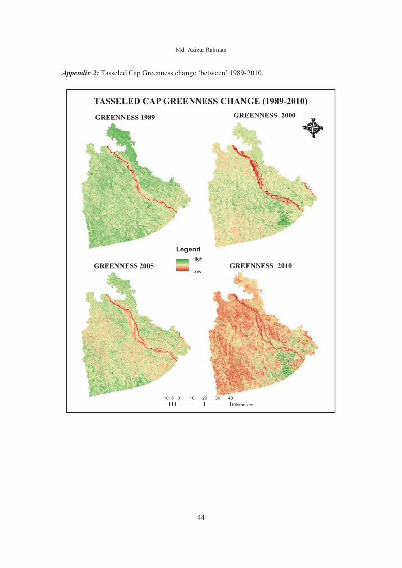
Md. Azizur Rahman
44
Appendix 2: Tasseled Cap Greenness change ‘between’ 1989-2010.
TASSELED CAP GREENNESS CHANGE (1989-2010)
GREENNESS 1989 GREENNESS 2000
Ì
10 0 10 20 30 405Kilometers
LegendHigh
Low GREENNESS 2010GREENNESS 2005

Water scarcity-induced change in vegetation cover along Teesta River catchments in Bangladesh: NDVI, Tasseled Cap and System dynamics analysis
45
TASSELED CAP WETNESS CHANGE (1989-2010)
LegendHigh
Low
ÌWETNESS 1989 WETNESS 2000
10 0 10 20 30 405Kilometers
WETNESS 2010WETNESS 2005
Appendix 3: Tasseled Cap Wetness change ‘between’ 1989-2010.
Appendix 4: Birth rate, death rate and annual growth rate in upstream (Source: SRS Bulletin October 2008, Registrar General of India, New Delhi (latest) and historic population growth in Bangladesh (downstream).

Md. Azizur Rahman
46
Historical demographical data of the whole country (Source: http://www.populstat.info/Asia/bangladc.htm)

Water scarcity-induced change in vegetation cover along Teesta River catchments in Bangladesh: NDVI, Tasseled Cap and System dynamics analysis
47
Appendix 5: Water demand change in upstream and downstream over time (Source: West Bengal State Action Plan on Climate Change Government of India, 2010). Appendix 6: Changes in Mean Monthly discharge of the Teesta River in the pre and post barrage operation (Source: Fakrul, and Higano 1999). Post Gozaldoba period Water Discharge (in m3 /second) Year Maximum Mean Minimum 1993-94 453 296 138 1994-95 633 412 190 1995-96 459 252 44 1996-97 478 259 39 1997-98 672 353 34 1998-99 364 200 36
Pre Gozaldoba period Water Discharge (in m3 /second) Year Maximum Mean Minimum 1978-79 721 541 361 1979-80 670 432 195 1980-81 522 330 137 198182 666 400 135 1982-83 652 415 177 1983-84 883 523 164 1984-85 795 488 182 1985-86 760 487 214 1986-87 660 425 190 1987-88 527 301 76 1988-89 667 397 127 1989-90 645 409 173 1990-91 729 427 125 1991-92 653 394 135

Md. Azizur Rahman
48
Appendix 7: System dynamic model for the study.
Teesta Riv er in Bangladesh
to brahmaputra riv er
Upstream water out take
Teesta Riv er in india
Brahmaputra riv er
Rain water in upstreamTotal catchment area in upstream
rain water inf olows in Downstream
Water inf lows in Upstream
Surf ace runof f in Upstream
water outtake downstream
rain water in downstreamUpstream out takelimiter
Water release f or downstream
Noname 4
Graph 1
~Anual av erage
rainf all in upstream
~Natural water f lows in upstream
Total catchment area in Downstream
~anual av erage rainf all
in downstream
~Noname 2
Ev arportation rain water in upstream
Table 1
Inf ilters of upstream rain water
Upstream ground water out take
Surf ace runof f in downstream
Ev aportation rain water in downstream
Inf ilteres of downstream rain water
Total ground water av ailable in upstream
Total population in upstream cachment area
Upstream population growth
~Birth rate in upstream per month
Upstream population decline
~Death rate in upstream
~population migration in
~population migration out
Total upstream water demand
Water exit to the bay of bengal
Upstream Ground water recharge
rest of the rain water in downstream
Graph 3
Graph 4
Graph 5
Total population in downstream cachment area
Downstream population growth
~Birth rate in
downstream per month
Downstream population decline
~Death rate in
downstream per month
~population migration
in downstream
~population migration out in downstream
Rest of the rain water in upstream
Graph 6
Total ground water av ailable in Downstream
Downstream Ground water in
Total water av ailable in downstream f rom dif f erent sources
Upstream water deman in agriculture
Land requirement per person
Woter in downstream
~Water required per capital
land per month in upstream
Graph 7
Total downstream water demand
water outtake downstream
Total downstream water demand
Arable land
Noname 5
Graph 16
Arable LandDownstream
Arable land reduction
Land requirement per person downstream
Vegetation
Vegetation growing in
Vegetation die naturally
v egetation out
v egetation reduced due to new settlements
Total population in downstream cachment area
Total study area
~Vegetation cov erd
Vegetation growth rate
Total water available in downstream from different sources
Water out in downstream
Graph 17
Total population in downstream cachment area
Graph 15
Total downstream water demand
Downstream water deman in agriculture
~Water required per capital land
per month in downstream
rest of the rain water in downstream
minimum water required per month per person in downstream
Water demand f or drinking and houshold in Downstream
Total ground water available in Downstream
Water demand in Downstream industry
~Amount of industrial
production in Downstream
~Downstream water demand in f orest and biodiv ersity
Water required per capital industrial production in Downstream
Graph 14
Total av ailable water f or use f rom teesta in upstream
Total water av ailable in upstream f rom dif f erent sources
condition
Graph 13
Total population in upstream cachment area
Water in Upstream Water out in upstream
minimum water required per month per person
Water demand f or drinking and houshold in upatream
Water demand in upstream industry
~Amount of industrial
production in upstream
~Upstream water demand in f orest and biodiv ersity
Water required per capital industrial production inupstream
Teeata Riv er Sy stem
Downstream Rain water Upstream Rain water
Upstream Ground water
Upstream Population
Total water av ailable and demand in downstream
Downstream Population
Downstream Ground water
Vegetation cov er change in Downstream
Total water av ailable and Demand in Upstream

Water scarcity-induced change in vegetation cover along Teesta River catchments in Bangladesh: NDVI, Tasseled Cap and System dynamics analysis
49
Appendix 8: Samples training area for naturally harvested and farmland in study area
Farmland
Farmland
Natural Harvested Land
Natural Harvested Land
Natural Harvested Land
Farmland
Farmland
Natural Harvested Land
Farmland
Natural Harvested Land
Natural Harvested Land
Farmland
Teeata Barage Irrigation Project
Natural Harvested and Farmlands sample area
6.5 0 6.5 13 19.5 263.25Kilometers
�Legend
Farmland
Natural Harvested Land
TBP Area

Md. Azizur Rahman
50
Appendix 9: Study area soil map.
89.061539752871
LegendFAO_Soil_Ban
FAOSOILAf46-1/2a
Ao78-3c
Ao79-a
Bd61-2c
Be81-2a
Be82-a
Bh10-2a
Gc9-3a
Gd25-2a
Ge12-1/2a
Ge38-2a
Ge50-2/3a
Ge51-2a
Ge52-3a
Ge53-3a
Jc50-2a
Jc52-2a
Je38-2a
Je71-2a
Je77-1/2a
Jt10-3a
Nd2-2b
Nd46-2ab
Od14-a
Rd29-1a
WAT
Grey Floodplain and Non Calcareous
Grey Floodplain and Non CalcareousGrey Floodplain and Non Calcareous
Grey Floodplain and Non Calcareous
Level Terrace soils
Grey Floodplain soils
Barind Tract soilsBarind Tract soils
Grey Floodplain soils
FAO Soil Map, Bangladesh Banglapedia
Study Area Soil Map
10 0 10 20 30 405Kilometers
Soil Map Comparison
�
Legend
Barind Tract soils
Grey Floodplain and Non Calcareous
Grey Floodplain soils
Level Terrace soils
Mixed Grey, Dark gray & brown Floodplain soils

Water scarcity-induced change in vegetation cover along Teesta River catchments in Bangladesh: NDVI, Tasseled Cap and System dynamics analysis
51
Appendix 10: Tasseled Cap spectral paths followed by a typical cultivated crop over the growing cycle and Greenness and Wetness angular measures of percentage cover (Crist, et al, 1986).
Appendix 11: Definition of NDVI values for land use classification
NDVI value for a given pixel is always follow certain scale of measurement that has a specific range from minus one (-1) to plus one (+1). Maximum value in this scale indicate the highest possible density of green leaves or biomass and close to zero (0) point to the no green vegetation and values below 0.1 correspond to barren areas or rock, sand, or snow; higher values from 0.2 to 0.3 indicate shrub and grassland; and temperate and tropical rainforests normally represents by values between 0.6 to 0.8 (Weier & Herring, 1999). However, negative values correspondence to the water whereas highest negative values reflects deep water and lowest negative values associate with less water bodies.

Md. Azizur Rahman
52
References Abbas A. T., B. M. (1984). The Ganges Water Dispute. Dhaka: University Press Ltd. Ahmad, S., & Slobodan, P., Simonovic, M. (2004). Spatial System Dynamics: New Approach for Simulation of Water Resources Systems. Journal of computing in civil engineering, 18 (4), 331-340. Annual report 2010-2011(March, 2011). Department of Agriculture and Cooperation Ministry of Agriculture, Government of India. Arsenic in Drinking Water and Resulting Arsenic Toxicity in India & Bangladesh (2004). World Health Organization. Retrieved August 8, 2012 from http://www.searo.who.int/en/Section314_4291.htm Bangladesh agriculture at a glance (n.d). Ministry of Agriculture, Government of the people’s republic of Bangladesh. Retrieved September 10, 2012 from http://www.moa.gov.bd/statistics/bag.htm Barbosa, H. A., Huete, A. R., & Baethgen, W. E. (2006). A 20 year study of NDVI variability over the Northeast Region of Brazil. Arid Environ, 67(2), 288-307. Batty, M. (2010). Integrated Models and Grand Challenges, ArcNews, Winter 2010/2011. Retrieved November 16, 2012 from http://www.esri.com/news/arcnews/winter1011articles/integrated-models.html Bhalme, H.N., & Mooley, D.A., (1980). Large-scale droughts/floods and monsoon circulation. Monthly Weather Review, 108 (8), 1197-1211. Boegh, E., Soegaard, H., Hanan, N., Kabat, P. & Lesh, L. (1999). A remote sensing study of the NDVI-T relationship and the transpiration from sparse vegetation in the sahel based on high-resolution satellite data. Remote Sensing of Environment, 69, 224-240. Braun & Abheuer. (2011). Floods in megacity environments: vulnerability and coping strategies of slum dwellers in Dhaka/Bangladesh. Natural Hazards, 58, 771-787. Braun, B., Shoeb, A.Z.M. (2008). Naturrisiken und Sozialkatastrophen in Bangladesch-Wirbelstu¨rme und U¨ berschwemmungen. Felgentreff, C., Glade, T. (eds). Naturrisiken und Sozialkatastrophen. Spektrum, Berlin, 383-393. Brolley, J.M., O'Brien, J.J., Schoo, J., & Zie, D., (2007). Experimental drought threat forecast for Florida. Agricultural and Forest Meteorology, 145, 84-96. Byun, H.R., & Wilhite, D.A., (1996). Daily quantification of drought severity and duration. Journal of Climate, 5, 1181-1201.

Water scarcity-induced change in vegetation cover along Teesta River catchments in Bangladesh: NDVI, Tasseled Cap and System dynamics analysis
53
Calculating Vegetation Indices (August 12, 2005). ENVI User's Guide. Retrieved November 30, 2012 from http://geol.hu/data/online_help/Calculating_Vegetation_Indices.html Caulfield, C. W., & Maj, S. P. (2001). A case for systems thinking and system dynamics. Proceedings of 2001 IEEE International Conference on Systems, Man and Cybernetics. IEEE, 5, 2793-2798. Ceccato, P., Flasse, S., & Gregoire, J.M., (2002b). Designing a spectral index to estimate vegetation water content from remote sensing data. Part 2. Validation and applications. Remote Sensing of Environment, 82, 198-207. Ceccato, P., Gobron, N., Flasse, S., Pinty, B., & Tarantola, S., (2002a). Designing a spectral index to estimate vegetation water content from remote sensing data: part 1 theoretical approach. Remote Sensing of Environment, 82, 188-197. Census of India: Sample Registration System (SRS) bulletin (2008). New Delhi: Registrar General of India. Central Statistical Organization, India, (2011). Annual report 2010-2011. Department of Agriculture and Cooperation, Ministry of Agriculture Government of India. Retrieved March 25, 2012 from http://agricoop.nic.in/Annual%20report2010-11/AR.pdf Chang, N.B., Yang, Y.J., Goodrich, J.A., Daranpob, A. (2010). Development of the Metropolitan Water Availability Index (MWAI) and short-term assessment with multi-scale remote sensing technologies. Journal of Environmental Management, 91, 1397-1413. Chen, D., Huang, J., & Jackson, T.J., (2005). Vegetation water content estimation for corn and soybeans using spectral indices from MODIS near- and short-wave infrared bands. Remote Sensing of Environment, 98, 225-236. Climate change (n. d.). Department of ecology state of Washington University. Retrieved October 28, 2012 from http://www.ecy.wa.gov/climatechange/whatis.htm Costanza, R. , & Voinov, A. (Eds.). (2004).Landscape Simulation Modeling: A Spatially Explicit, Dynamic Approach Series (Modeling Dynamic Systems). New York: Springer. Country strategy and program 2006-2010. Asian Development Bank, Dhaka, Bangladesh: Bangladesh Resident Mission. Retrieved March 13, 2012 from http://www.adb.org/sites/default/files/pub/2005/csp-ban-2005.pdf Crist, E. P., and Richard C. Cicone (1984). A Physically-Based Transformation of Thematic Mapper Data-The TM Tasseled Cap. IEEE Transactions on Geoscience and Remote Sensing, 22 (3), 256-263. Crist, E. P., R. Laurin, and R. C. Cicone. (1986a). Vegetation and soils information contained in transformed Thematic Mapper data. Proceedings of IGARSS' 86 Symposium. Paris: European Space Agency, 1465-70. Retrieved December 14, 2012 form http://www.ciesin.org/docs/005-419/005-419.html Crist, E.P. & Cicone, R.C. (1986b). Application of the Tasseled Cap Concept to Simulated Thematic Mapper Data. Photogrammetric Engineering and Remote Sensing, 50, 343-352.

Md. Azizur Rahman
54
Dammed river, Dead River: A case study on Teesta (2011). Retrieved September 1 , 2012 from http://nilphamari.info/?p=44 Dow, K. & Edward, R. (2005). Linking Water Scarcity to Population Movements: From Global Models to Local Experiences. For the Poverty and Vulnerability Programme Stockholm Environment Institute (SEI), Stockholm, Sweden. Environmental Information System (2006). Forests, Environment & Wildlife Management Department, Government of Sikkim. Retrieved August 10, 2012 from http://sikenvis.nic.in/soer/Water%20Resources.pdf Fensholt, R. & Rasmussen, K. (2011). Analysis of trends in the Sahelian ‘rain-use efficiency’ using GIMMS NDVI, RFE and GPCP rainfall data. Remote Sensing of Environment, 115, 438-451. Find and analysis geo-spatial data, High resolution digital soil map of the world (2007). FAO, GeoNetwork. Retrieved December 13, 2012 from http://www.fao.org/geonetwork/srv/en/metadata.show?id=14116 Forrester, J., (1961). Industrial dynamics. Boston: MIT press, 464p Fotheringham, S. & Rogerson, P. (2005). Spatial analysis and GIS. John St, London: Taylor & Francis Ltd. Gao, B.C., (1996). NDWI e a normalized difference water index for remote sensing of vegetation liquid water from space. Remote Sensing of Environment, 58, 257-266. Gibbs, W.J., & Maher, J.V., (1967). Rainfall Deciles as Drought Indicators. Bureau of Meteorology Bulletin. 48. Ghulam, A., Qin, Q.M., Teyip, T., & Li, Z.L., (2007). Modified perpendicular drought index (MPDI): a real-time drought monitoring method. Journal of Photogrammetry & Remote Sensing, 62, 150-164 Goodchild, M. F., & Longley P. A. (2005). The future of GIS and spatial analysis. In Geographical information systems: Principles, techniques, management and applications Hoboken, N.J: John Wiley and Sons. Grant, J., Carter , F. L., (2011). Calculating Vegetation Indices from Landsat 5 TM and Landsat 7 ETM+ Data. Colorado state university, USA. Ground water scenario (2009-2010) of India (June 2010). Central ground water board, ministry of water resource, Government of India. Guo-yu, Q., Jin, Y., & Geng, S. (2012). Impact of Climate and Land-Use Changes on Water Security for Agriculture in Northern China. Journal of Integrative Agricultur, 11(1), 144-150. Guttman, N.B., (1998). Comparing the Palmer drought index and the standardized precipitation index. Journal of American Water Resources Association, 34, 113-121.

Water scarcity-induced change in vegetation cover along Teesta River catchments in Bangladesh: NDVI, Tasseled Cap and System dynamics analysis
55
Guttman, N.B.,Wallis, J.R., & Hosking, J.R.M., (1992). Spatial comparability of the Palmer drought severity index. Water Resources Bulletin, 28, 1111-1119. Habiba, U., Shaw, R., Takeuchi, Y. (2012). Farmer’s perception and adaptation practices to cope with drought: Perspectives from Northwestern Bangladesh. International Journal of Disaster Risk Reduction. http://dx.doi.org/ 10.1016/j.ijdrr.2012.05.004. Hanif, Abu, S (1995). Hydro- Geomorphic Characteristics of the Teesta Flood Plain. Bangladesh: Ph.D. Thesis. Department of Geography, University of Rajshahi, Bangladesh. Hein, L., de Ridder, N., Hiernaux, P., Leemans, R., de Wit, A. & Schaepman, M. (2011). Desertification in the Sahel: Towards better accounting for ecosystem dynamics in the interpretation of remote sensing images. Journal of Arid Environments, 75, 1164-1172. Huang, C., Wylie, L., Yang, C., Homer, & Zylstra, G., (2002). Derivation of a tasseled Cap transformation based on Landsat 7 at satellite reflectance. International Journal of Remote Sensing, 23, 1741-1748. Hunt, E.R., Rock, B.N., & Nobel, P.S. (1987). Measurement of leaf relative water content by infrared reflectance. Remote Sensing of Environment, 22, 429-43. Haraldsson V. Haraldsson. (2004). Introduction to Systems and Causal Loop Diagrams. Report in Ecology and Environmental Engineering, Lund University, Sweden. International decade for action ‘water for life’ 2005-2015: Water scarcity. UNDESA. Retrieved April 19, 2012 from https://www.un.org/waterforlifedecade/scarcity.shtml Islam, M. F., Higano, Y. (1999). International Environmental Issue between India and Bangladesh: Environmental and Socio-economic Effects on the Teesta River Area. European Regional Science Association, ERSA conference papers. Islam, M. F., Higano, Y. (2001). Equitable Sharing of Bilateral International. Water: A Policy Measure for Optimal Utilization of the Teesta River. Studies in Regional Science, 32(1), 17-32. Islam, N., Azam, M. A., & Islam, R. (2004). Teesta River water sharing: a case study in Teesta barrage project, Local Government Engineering Department (LGED), Dhaka, Bangladesh. Islam, S. et al. (Eds). (2006). Drought in Bangladesh. Banglapedia, national encyclopedia of Bangladesh. Retrieved April 20, 2012 from http://www.banglapedia.org/HT/D_0284.HTM Iyob, B. (2005). Mapping Vegetation Using Landsat TM and ETM+ in Eritrea. Student thesis, Oregon State University, USA. Retrieved May 2, 2012 from http://ir.library.oregonstate.edu/xmlui/handle/1957/3918?show=full Jackson et.al (2004). Vegetation water content mapping using Landsat data derived normalized difference water index for corn and soybeans. Remote sensing of Environment, 92, 475-482.

Md. Azizur Rahman
56
Jensen, J. R., (1986). Introductory Digital Image Processing. Prentice-Hall, New Jersey, p. 379. Katz, R.W., & Glantz, M.H., (1986). Anatomy of a rainfall index. MonthlyWeather Review, 114 (4), 764-771. Kauth, R.J., Lambeck, P.F. Richardson, W., Thomas, G.S. & Pentland, A.P., (1979). Feature extraction applied to agricultural Crops as seen by Landsat. Houston TX: LACIE Symposium , NASA, 705-721. Keetch, J.J., & Byram, G., (1968). A Drought Index for Forest Fire Control. Res. Paper SE-38. U.S. Department of Agriculture, Forest Service, Southeastern Forest Experiment Station, Asheville, NC. Kimura, R., (2007). Estimation of moisture availability over the Liudaogou river basin of the Loess Plateau using new indices with surface temperature. Journal of Arid Environments, 70, 237-252. Kogan, F.N. (1995) Application of vegetation index and Brightness temperature for drought detection. Advances in space research, 15, 91-100. Land Cover trend project (n. d.). United States Geological Survey (USGS). Retrieved August 29, 2012 from http://landcovertrends.usgs.gov/main/about.html Land-use and land-cover change (2010). The Encyclopedia of Earth. Retrieved October 28, 2012 from http://www.eoearth.org/article/Land-use_and_land-cover_change Le, Q. B., Park, S. J., Vlek, P. L. G. (2010). Land Use Dynamic Simulator (LUDAS): A multi-agent system model for simulating spatio-temporal dynamics of coupled human-landscape system 2. Scenario-based application for impact assessment of land-use policies. Ecological Informatics, 5, 203-221. Liu, A.X., Liu, Z.J., Wang, C.Y., Niu, & Yan, D.M. Z. (2003). Monitoring of desertification in central Asia and western China using long term NOAA-AVHRR NDVI time-series data. Geoscience and Remote Sensing Symposium, 4, 2278-2280. Liu, Y. (2009). Modelling Urban Development with Geographical Information Systems and Cellular Automata. London: Taylor & Francis. Maeda, E.E, Petri K.E., Pellikka, Barnaby J.F., Clark, Siljander, M. (2011). Prospective changes in irrigation water requirements caused by agricultural expansion and climate changes in the eastern arc mountains of Kenya. Journal of Environmental Management, 92, 982-993. Maguire, D. J., Goodchild, M. F., Batty, M. (2005). GIS, Spatial Analysis, and Modeling. New York: ESRI press.

Water scarcity-induced change in vegetation cover along Teesta River catchments in Bangladesh: NDVI, Tasseled Cap and System dynamics analysis
57
Majumdar, B. S. (1999). The information technology-based improved management system for the Teesta Barrage project. FAO Corporate document repository, CMC Ltd, Pune, India. Retrieved April 27, 2012 from http://www.fao.org/docrep/003/X6626E/x6626e16.htm Mas. J.F., (1999). Monitoring land-cover changes: a comparison of change detection techniques. International Journal of Remote Sensing, 20,139-152. Mbugua, A., & Snijders, J.M. (2011). Study Report on Water Scarcity in Northern Bangladesh. Parbatipur, Dinajpur: VSO International volunteers and Gram Bikash Kendra (GBK). McFeeters, S.K., (1996). The use of the Normalized Difference Water Index (NDWI) in the delineation of open water features. International Journal of Remote Sensing, 17 (7), 1425-1432. McKee, T.B., Doesken, N.J., & Kleist, J., (1993). The Relationship of Drought Frequency and Duration to Time Scales. Eighth Conference on Applied Climatology. American Meteorological Society. Michael J. , & Radzicki Robert A. T. (2008). Origin of System Dynamics. Retrieved March 30, 2012 from http://www.systemdynamics.org/DL-IntroSysDyn/origin.htm Mishra, A.K., & Sing, V.P. (2011). Drought modeling-A review. Journal of Hydrology, 403, 157-175. Mondal, M.S., Saleh, A.F.M. (2003). Evaluation of some deep and shallow tubewell irrigated schemes in Bangladesh using performance indicators. Agricultural Water Management, 58(3), 193-207. Moulin, S., Kergoat, L., Viovy, N., & Dedieu, G. (1997). Global scale assessment of vegetation phenology using NOAA/AVHRR satellite measurements. Climate, 10(6), 1154-1170. Mullick, .M.R. A. , Babel1, M. S., & Perret, S. R. (2011a). Discharge-based economic valuation of irrigation water: Evidence from the Teesta river, Bangladesh. Irrigation and drainage, 60, 481-492. Mullick, .M.R. A. , Babel1, M. S., & Perret, S. R. (2010b). Flow characteristics and environmental flow requirements for the Teesta River, Bangladesh: Proc. of International Conference on Environmental Aspects of Bangladesh (ICEAB10), Japan. Retrieved April 16, 2012 from http://benjapan.org/iceab10/42.pdf Murad, H. & Islam, A. K. M. S. (2011). Drought assessment using remote sensing and GIS in North-west region of Bangladesh. 3rd International Conference on Water & Flood Management (ICWFM-2011). Narasimhan, B., & Srinivasan, R., (2005). Development and evaluation of soil moisture deficit index (SMDI) and evapotranspiration deficit index (ETDI) for agricultural drought monitoring. Agricultural and Forest Meteorology, 133, 69-88
Md. Azizur Rahman
58
Nayak, A. & Jeffrey, A. (2011). Geographical Thought: An Introduction to Ideas in Human Geography. England: Pearson Education Ltd. NDVI (n.d.). Department of Geography and the Environment, Villanova University, USA. Retrieved December 10, 2012 from http://www47.homepage.villanova.edu/guillaume.turcotte/studentprojects/arboretum/NDVI.htm Ogunseitan, A. O. (2008). Scarcity on a Water Planet (eds). African Journal of Environmental Science and Technology, 2 (12). Olivier, et al (2012). Disaggregation of SMOS Soil Moisture in Southeastern Australia. Ieee transactions on geoscience and remote sensing, 50(5), 1556-1571. Palmer,W.C., (1968). Keeping track of crop moisture conditions, nationwide: the crop moisture index. Weatherwise 21 (4), 156-161. Palmer, W.C., (1965). Meteorological Drought. Research Paper, 45. U.S. Department of Commerce Weather Bureau, Washington, DC. Paul, B.K., (1998). Coping mechanisms practiced by drought victims (1994/ 95) in North Bengal, Bangladesh. Applied Geography, 18, 355-73. Peñuelas, J., Pinol, J., Ogaya, R., & Filella, I., (1997). Estimation of plant water concentration by the reflectance water Index WI (R900/R970). International Journal of Remote Sensing, 18, 2869-2875. Petrosa, G., Antonisb, M., Marianthia, T. (2011). Development of an adapted empirical drought index to the Mediterranean conditions for use in forestry. Agricultural and Forest Meteorology, 151, 241-250. Sarker, D.C., Pramanik, B.K., Zerin, A.I. & Ara, I. (2011). Climatic Impact Assessment: A Case Study of Teesta Barrage Irrigation Project in Bangladesh. International Journal of Civil & Environmental Engineering, 11(1), 99-110. Shafer, B.A., & Dezman, L.E., (1982). Development of a Surface Water Supply Index (SWSI) to Assess the Severity of Drought Conditions in Snowpack Runoff Areas. Proc. of the Western snow Conference. Shafie, H. Shantana, R. H., Rashid, A. K. M., Lisa, K.S., Mita, H. A. (2009). Endowed wisdom: knowledge of nature and coping with disaster in Bangladesh. Dhaka: Comprehensive Disaster Management Programme (CDMP). Shahid, S., & Behrawan, H. (2008). Drought risk assessment in the western part of Bangladesh. Journal of the International Society for the Preven- tion and Mitigation of Natural Hazards, 46, 391-413.

Water scarcity-induced change in vegetation cover along Teesta River catchments in Bangladesh: NDVI, Tasseled Cap and System dynamics analysis
59
Statistical Pocket Book (2008). Bangladesh Bureau of Statistics. Retrieved August, 2012 fromhttp://www.bbs.gov.bd/WebTestApplication/userfiles/Image/SubjectMatterDataIndex/pk_book_09.pdf Rahman, A. (2010). Application of GIS in Ecotourism development: a case study of Sundarbans Bangladesh. Student thesis, Department of Human geography, Mid Sweden University, Sweden. Rahman, M.M. (2005). Bangladesh-From a country of flood to a country of water scarcity-sustainable perspective for solution. Seminar on Environment and development, Hamburg, Germany, entwicklungsforum Bangladesh e.v. Retrieved February 3, 2012 from http://users.tkk.fi/~mizanur/Rahaman_Hamburg.pdf Reaz, A. M, Mukand S. B., & Sylvain R. P. (2010). Proc. of International Conference on Environmental Aspects of Bangladesh (ICEAB10), Japan. Rock, B.N., Vogelman, J.E., Williams, D.L., Vogelman, A.F., & Hoshizaki, T., (1986). Remote detection of forest damage. Bioscience, 36, 439-445. Tahira Abbasova (2010). Detection and analysis of changes in desertification in the Caspian Sea Region. Master’s thesis, Department of Physical Geography and Quaternary Geology, Stockholm University, Sweden. Tasseled Cap transformation: Mississippi Coastal Corridor (July 24, 2000). Computer Geospatial technologies center, Mississippi State University. Retrieved October 25, 2012 from http://www.ncrste.msstate.edu/archive/publications/posters/ncrste_tg002-9.pdf The Thematic Mapper And Enhanced Thematic Mapper. NASA. Retrieved March 21, 2012 from http://landsat.gsfc.nasa.gov/about/etm+.html and http://landsat.gsfc.nasa.gov/about/tm.html Toomey, M. (2011). Introduction to Remote Sensing. Lab Assignment #2 - Spectral Transformations, University of California, Santa Barbara, USA. Retrieved August 15, 2012 from http://geog.ucsb.edu/~mtoomey/geog115b/Lab2Geog115BW2011.pdf Tucker, C. & Choudhry, B. (1987). Satellite remote sensing of drought conditions. Remote Sensing of Environment, 23, 243-251. Tucker, C., Pinzon, J., Brown, M., Slayback, D., Pak, E; Mahoney, R., Vermote, E. & El Saleous, N. (2005). An extended AVHRR 8 km NDVI dataset compatible with MODIS and SPOT vegetation data. International Journal of Remote Sensing, 26, 4485-4498 Van Rooy, M.P. (1965). A rainfall anomaly index independent of time and space. Notos 14, 43-48. Vogelmann, J. E., Howard, L. S. M., Yang, C. R., Larson, B. K., Wylie & Driel, V. J. N. (2001). Completion of the 1990’s National Land Cover Data Set for the conterminous United States. Photogrammetric Engineering and Remote Sensing, 67, 650-662.
Md. Azizur Rahman
60
Wahid S. M., Mukand, S., Babel, Gupta, A.S. & Roberto S. C. (2007). Spatial assessment of groundwater use potential for irrigation in Teesta Barrage Project in Bangladesh. Hydrogeology Journal, 15, 365-382. Wang, X. (2004). Integrating GIS, simulation models, and visualization in traffic impact analysis. Computers, Environment and Urban Systems, 29, 471-496. Water resources. State of Environment Sikkim (SES). (2007). Retrieved April 15, 2012 from http://www.sikkimforest.gov.in/soer/Water%20Resources.pdf Water Scarcity in Bangladesh and South Asia: Dynamics of Conflict and Cooperation (2012). The Peace Research Institute Oslo (PRIO). Retrieved April 15, 2012 from http://www.prio.no/Projects/Project/?x=969 Weatherheada, E. K., Howdenb, N.J.K. (2009). The relationship between land use and surface water resources in the UK. Land Use Policy 26, 243-250. Weier J., & Herring D., (1999). Measuring Vegetation (NDVI & RVI). Retrieved February 2, 2012 from http://earthobservatory.nasa.gov/Features/MeasuringVegetation/ West Bengal State Action Plan on Climate Change (2010). Government of India. Westerberg, L., Holmgren, K,. Börjeson, L., Håkansson, K., Laulumaa, V., Ryner, M. & Öberg, H. (2010).The development of the ancient irrigation system at Engaruka, northern Tanzania: physical and societal factors. The Geographical Journal, 176 (4), 304-318. What is GIS? Overview. Environmental System Research Institute (ESRI). Retrieved April 11, 2012 from http://www.esri.com/what-is-gis/overview Zeng, B., & Yang, T. B. (2008). Impacts of climate warming on vegetation in Qaidam Area from 1990 to 2003. Environmental Monitoring and Assessment,144, 403-417. Retrieved December 11, 2011 from http://link.springer.com/article/10.1007%2Fs10661-007-0003-x?LI=true Zhang, Q. (2009). Spatial-temporal patterns of urban growth in Shanghai China: monitoring, analysis, and simulation. PhD thesis, Royal Institute of Technology (KTH), Sweden: KTH publication database, DiVA. Retrieved September 21, 2012 from http://kth.diva-portal.org/smash/record.jsf?pid=diva2:286574 Zinyowera, C. M., Dokken, J. D., Watson, T. R., & Moss, H.R. (Eds). (2007). The regional impacts of climate change: an assessment of vulnerability. Intergovernmental Panel on Climate Change (IPCC). Retrieved August 8, 2012 from http://www.ipcc.ch/pdf/special-reports/spm/region-en.pdf Zribi, M., Anguela, T. P., Duchemin, B., Lili, Z., Wagner, W., Hasenauer, S. & Chehbouni, A. (2010). Relationship between soil moisture and vegetation in the Kairouan plain region of Tunisia using low spatial resolution satellite data. Water resources research, 46. Zug, S (2006). Monga - Seasonal Food Insecurity in Bangladesh - Bringing the Information Together. The Journal of Social Studies, 111.