Wasserman, S. & Faust, K. (1994). Social network analysis ... · PDF fileapplications. New...

PAD-637 Reading Notes Week #3-2/8/10-Lunix, Junesoo & Steve – pg. 2 of 22

Wasserman, S. & Faust, K. (1994). Social network analysis: Methods and applications. New York: Cambridge University Press.

Part II: Mathematical Representations of Social Networks

Chapter 3: Notation for Social Network Data (pp. 69-91) Three notational schemes: Graph Theoretic, Sociometric, and Algebraic Graph Theoretic Notation (pp. 71-76)

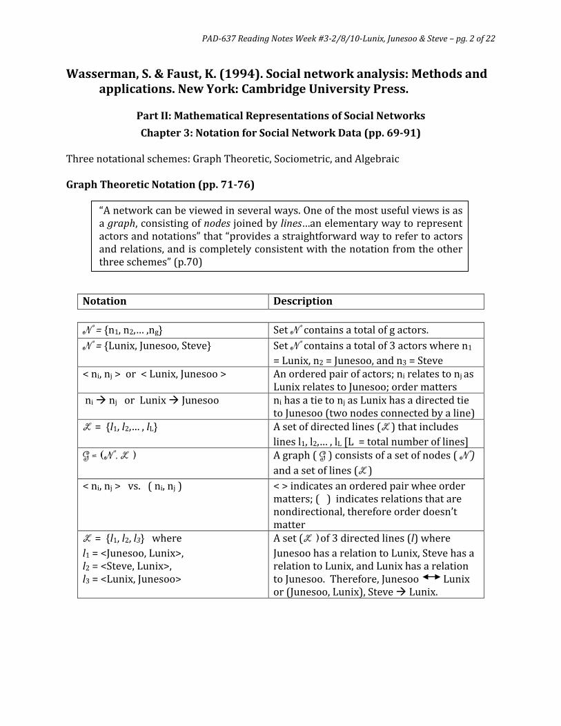
“A network can be viewed in several ways. One of the most useful views is as a graph, consisting of nodes joined by lines…an elementary way to represent actors and notations” that “provides a straightforward way to refer to actors and relations, and is completely consistent with the notation from the other three schemes” (p.70)

Notation Description

N = {n1, n2,… ,ng} Set N contains a total of g actors. N = {Lunix, Junesoo, Steve} Set N contains a total of 3 actors where n1

= Lunix, n2 = Junesoo, and n3 = Steve < ni, nj > or < Lunix, Junesoo > An ordered pair of actors; ni relates to nj as

Lunix relates to Junesoo; order matters ni nj or Lunix Junesoo ni has a tie to nj as Lunix has a directed tie

to Junesoo (two nodes connected by a line) L = {l1, l2,… , lL} A set of directed lines (L ) that includes

lines l1, l2,… , lL [L = total number of lines] G = (N , L ) A graph ( G ) consists of a set of nodes ( N )

and a set of lines (L ) < ni, nj > vs. ( ni, nj ) < > indicates an ordered pair whee order

matters; ( ) indicates relations that are nondirectional, therefore order doesn’t matter

L = {l1, l2, l3} where l1 = <Junesoo, Lunix>, l2 = <Steve, Lunix>, l3 = <Lunix, Junesoo>

A set (L )of 3 directed lines (l) where Junesoo has a relation to Lunix, Steve has a relation to Lunix, and Lunix has a relation to Junesoo. Therefore, Junesoo Lunix or (Junesoo, Lunix), Steve Lunix.


Sociometric Notation (pp. 77-84)

“…by far the most common in the social network literature… Sociomatrices began to be used more than fifty years ago after their introduction by Moreno (1934)” (p. 70).

“Sociometry is the study of positive and negative affective relationa, such as liking/disliking and friends/enemies, among a set of people. A social network data set consisting of people and measured affective relations between people is often referred to as sociometric.

Relational data are often presented in two-way matrices termed sociomatrices. The two dimensions of a sociomatrix are indexed by the sending actor (the rows) and the receiving actors (the columns). Thus, if we have a one-mode network, the sociomatrix will be square” (p. 77).

Luni

x

June

soo

Stev

e Lunix - 1 0 Junesoo 1 - 0 Steve 1 0 -

An example of a sociomatrix of the relations described

in the section on Graph Theoretic Notation (above).

“A sociomatrix for a dichotomous relation is exactly the adjacency matrix for the graph (or sociogram) quantifying the ties between the actors for the relation in question” (p. 77). “The line between sociometric and graph theoretic approached to social network analysis began to become blurred during the early history of the discipline, as computers began to play a bigger role in data analysis…much to the dismay of Moreno (1946)” (p. 70).

Notation Description

N = {n1, n2,… ,ng} Set N contains a total of g actors. X Single-valued, directional relation in N X The resultant sociomatrix Xij The value of the tie from ni to nj on relation X Xijr The value of any tie from ni to nj on relation Xr


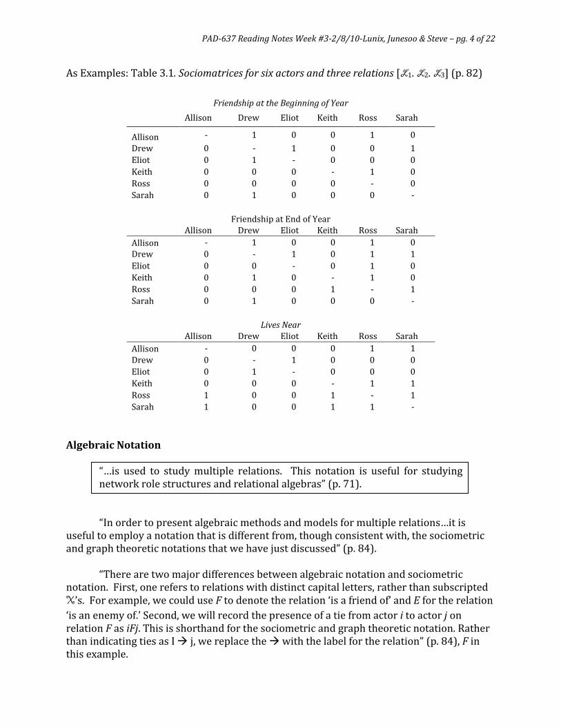
As Examples: Table 3.1. Sociomatrices for six actors and three relations [L1. L2. L3] (p. 82)

Friendship at the Beginning of Year

Allison Drew Eliot Keith Ross Sarah

Allison - 1 0 0 1 0 Drew 0 - 1 0 0 1 Eliot 0 1 - 0 0 0 Keith 0 0 0 - 1 0 Ross 0 0 0 0 - 0 Sarah 0 1 0 0 0 -

Friendship at End of Year

Allison Drew Eliot Keith Ross Sarah Allison - 1 0 0 1 0 Drew 0 - 1 0 1 1 Eliot 0 0 - 0 1 0 Keith 0 1 0 - 1 0 Ross 0 0 0 1 - 1 Sarah 0 1 0 0 0 -

Lives Near Allison Drew Eliot Keith Ross Sarah Allison - 0 0 0 1 1 Drew 0 - 1 0 0 0 Eliot 0 1 - 0 0 0 Keith 0 0 0 - 1 1 Ross 1 0 0 1 - 1 Sarah 1 0 0 1 1 -

Algebraic Notation

“…is used to study multiple relations. This notation is useful for studying network role structures and relational algebras” (p. 71).

“In order to present algebraic methods and models for multiple relations…it is useful to employ a notation that is different from, though consistent with, the sociometric and graph theoretic notations that we have just discussed” (p. 84). “There are two major differences between algebraic notation and sociometric notation. First, one refers to relations with distinct capital letters, rather than subscripted X’s. For example, we could use F to denote the relation ‘is a friend of’ and E for the relation ‘is an enemy of.’ Second, we will record the presence of a tie from actor i to actor j on relation F as iFj. This is shorthand for the sociometric and graph theoretic notation. Rather than indicating ties as I j, we replace the with the label for the relation” (p. 84), F in this example.


“Unfortunately, this notational scheme can not handle valued relations or actor attributes” (p. 85). Two Sets of Actors (Two-Mode Networks) The first actor is the “sender”, the second the “receiver” in both sets. However, they are designated differently in the two transactions: N is the first set of actors, and M is the second set. Actors (dyads, triads and the like) in both sets (N & M) can also interact in the other set of actors, thereby creating separate and distinct sociomatrices. Sociometric Notation The discussion above illustrates the convention described by Wasserman & Faust (1994, p. 88) found below. To be discussed in class.

M

Mr. Jones

Ms. Smith

Ms. Davis

Mr. White

N

Allison 1 0 0 0 Drew 0 1 0 0 Eliot 0 0 1 0 Keith 0 0 0 1 Ross 0 0 1 0 Sarah 0 1 0 0


Chapter 4: Graphs and Matrices (pp. 92-166)

Xiaohui Lu

4.1 Why graph?

Graphs have been widely used in social network analysis (SNA) as a means of formally representing social relations and quantifying important social structural properties.

Graph theory is useful in SNA:

1. Graph theory provides a vocabulary, which can be used to label and denote many social structural properties.

2. Graph theory gives us mathematical operations and ideas with which many of these properties can be quantified and measured.

3. Graph theory gives us the ability to prove theorems about graphs, and hence, about representation of social structure.

4. Gives us a representation of a social network as a model of a social system.

The visual representation of data allows researchers to uncover patterns that might otherwise go undetected

.

4.2 Graphs

A graph G = (N, L) consists of a set of nodes: N = {n1, n2, …, ng}, and a set of lines, L = {l1, l2, …, lm} between pairs of nodes. (i.e. lk = (ni, nj)).

A loop is a line between a node and itself.

A simple graph is a graph has no loops and includes no more than one line between a pair of nodes.

Two nodes are adjacent if there is a line connects them. A node is incident with a line, and the line is incident with the node, if the line connects the nodes.

A trivial graph is a graph with only one node and empty line set.

An empty graph is a graph with at least one node and no lines.

4.2.1 Subgraphs, Dyads, and Triads

A graph Gs(Ns, Ls) is a subgraph of G(N, L) if Ns ⊆ N, and Ls ⊆ L.

Node-generated subgraph: a subgraph with its line set Ls includes all lines from L that are between pairs of nodes in its node set Ns.


Line-generated subgraph: a subgraph with its node set Ns includes all nodes from N that are incident with lines in its line set Ls.

Dyad: a subgraph consisting of a pair of nodes and the possible line

Triads: a subgraph consisting of

between the nodes.

three nodes and the possible lines

among them.

4.2.2 Nodal Degree

The degree of a node n, denoted by d(n), is the number of lines that are incident with n, or, the number of nodes adjacent to n.

The mean degree d is the average degree of the nodes in the graph.

d

Variance of the degree: SD2 = ∑ �𝑑𝑑(𝑛𝑛 i)− d �2𝑔𝑔𝑖𝑖=1

𝑔𝑔

= 2𝑚𝑚𝑔𝑔

, where m is the number of lines and g is the number of nodes.

4.2.3 Density of graphs

Density : the ratio of the number lines in a graph to the maximum number of lines that can be present.

∆ = 𝑚𝑚𝑔𝑔(𝑔𝑔−1)/2

= 2𝑚𝑚𝑔𝑔(𝑔𝑔−1)

, where m is the number of lines in the graph, g is the number of nodes in the graph.

There are g(g-1)/2 possible lines in the graph. No loops are allowed.

If any two nodes in a graph are adjacent then the graph is called complete graph or clique.

4.2.5 Walks, Trails, and Paths

Walk: a sequence of nodes and lines, starting and ending with nodes, in which each node is incident with the lines following and preceding it in the sequence.

Trail: a walk in which all of the lines are distinct.

Path: a walk in which all nodes and all lines are distinct.

Closed walk: a walk begins and ends at the same node.

Every path is a trail and every trail is a walk.


Cycle: a closed walk of at least three nodes in which all lines are distinct, and all nodes except the beginning and ending node are distinct.

Tour: a closed walk in which each line in the graph is used at least once.

The number of lines in a walk (resp. trail, path) is the length of the walk (resp. trail, path).

4.2.6 Connected Graphs and Components

Connected graph: there is a path between all pairs of nodes in the graph.

There is path between ni and nj, we say that nj is reachable by ni.

A component of a graph is a maximal connected subgraph.

Only one component in a graph => the graph is connected.

More than one component in a graph => the graph is disconnected.

4.2.7 Geodesics, Distance, and Diameter

Geodesic: a shortest path between two nodes.

Distance between two nodes ni and nj, denoted d(i, j), is the length of the shortest path between the two nodes.

Eccentricity of a node ni is the largest geodesic distance (maxjd(i, j)) between that node and any other nodes.

The diameter of a connected graph is the length of the largest geodesic (maximaxjd(i, j)) between any pair of nodes.

4.2.8 Connectivity of Graphs

A node ni in a connected graph is called a cutpoint, if its removal disconnects the graph.

A line li in a connected graph is called a bridge, if its removal disconnects the graph.

The node-connectivity of a graph, K(G), is the minimum number K of nodes that must be removed to make the graph disconnected, or to leave a trivial graph.

The line-connectivity of a graph, λ(G), is the minimum number λ of lines that must be removed to make the graph disconnected, or to leave a trivial graph.


4.2.9 Isomorphic Graphs and Subgraphs

Two graphs G = (N, L) and G′ = (N′, L′) are called isomorphic, if there is a one-to-one mapping function f from N onto N′ such that any two nodes n1, n2 ∈ N are adjacent iff f(n1) and f(n2) are adjacent.

If two graphs are isomorphic, then they are identical on all graph theoretic properties, such as two isomorphic graphs have the same number of nodes, lines, density, diameter, and so on.

4.2.10 Special Kinds of Graphs

The complement G = (N, L ) of a graph G = (N, L) has the same node set as its node set

and two nodes are adjacent in G

A graph that is connected and is acyclic is called a tree.

iff they are NOT adjacent in G.

If the nodes in a graph G = (N, L) can be partitioned into two subsets, N = N1 ∪ N2, and any two adjacent nodes belong to different subsets, then G is a bipartite graph.

A bipartite graph with any two vertices from different partitions are adjacent is called complete bipartite graph.

4.3 Directed graph

A directed graph, or digraph, G = (N, L) is a graph such that each arc is an ordered pair of distinct nodes.

lk = <ni, nj> is different from lk’ = <nj, ni>.

4.3.1 Subgraphs – Dyads

There are three isomorphism classes of dyads:

Null dyads: have no arcs, in either direction, between the two nodes.

Asymmetric dyads: have an arc between the two nodes going in one direction or the other, but not both.

Mutual dyads: have two arcs between the two nodes, one going in one direction and the other going in the opposite direction.

4.3.2 Nodal Indgree and Outdegree


The indegree of a node, dI(ni), is the number of nodes that are adjacent to ni, or the number of arcs terminating at ni.

The outdegree of a node, dO(ni), is the number of nodes that are adjacent from ni, or the number of arcs originating with node ni.

Mean indegrees dI and outdegrees dO :

dI = ∑ 𝑑𝑑I(𝑛𝑛 i)𝑔𝑔𝑖𝑖=1

𝑔𝑔

dO

Since the indegrees count arcs incident from the nodes, and the outdegrees count arcs incident to the nodes, ∑ 𝑑𝑑I(𝑛𝑛i)𝑔𝑔

𝑖𝑖=1 = ∑ 𝑑𝑑O(𝑛𝑛i)𝑔𝑔𝑖𝑖=1 = m, number of lines in a graph.

= ∑ 𝑑𝑑O(𝑛𝑛 i)𝑔𝑔𝑖𝑖=1

𝑔𝑔

dI =

Variance of indgrees SDI2and outdegrees SDO2:

dO = m.

SDI2 = ∑ (𝑑𝑑I(𝑛𝑛𝑖𝑖 )− di )𝑔𝑔𝑖𝑖=1

𝑔𝑔

SDO2 = ∑ (𝑑𝑑O(𝑛𝑛𝑖𝑖 )− do )𝑔𝑔𝑖𝑖=1

𝑔𝑔

A node ni in a digraph is a(n)

• isolate if dI(ni) = do(ni) = 0, • transmitter if dI(ni) = 0 and do(ni) > 0, • receiver if dI(ni) > 0 and do(ni) = 0, • carrier of ordinary if dI(ni) > 0 and do(ni) > 0.

4.3.3 Density of a Directed Graph

The density, ∆, of a digraph is equal to the proportion of arcs present in the graph.

∆ = 𝑚𝑚𝑔𝑔(𝑔𝑔−1)

, where m = the number of arcs in the digraph, g = the number of nodes.

4.3.5 Directed Walks, Paths, Semipaths

A directed walk is a sequence of alternating nodes and arcs so that each arc has its origin at the previous node and its terminus at the subsequent node – pointing in the same direction.


A directed trail is a directed walk in which no arc is included more than once.

A directed path is a directed walk in which no node and no arc is included more than once.

A semiwalk is a sequence of nodes and irrelevant direction of arcs.

A semipath is a sequence of distinct nodes with irrelevant direction of arcs.

Every path is a semipath, but not every semipath is a path

A cycle in a digraph is a closed directed walk of at least three nodes in which all nodes except the first and the last are distinct.

.

A semicycle in a digraph is a closed directed semiwalk of at least three nodes in which all nodes except the first and the last are distinct.

4.3.6 Reachability and Connectivity in Digraphs

If there is a directed path from ni to nj in a digraph, then node nj is reachable from node ni.

A pair of nodes, ni and nj, is:

• weakly connected: joined by a semipath; • unilaterally connected: joined by a path from ni to nj, or a path from nj to ni; • strongly connected: joined by a path from ni to nj, and a path nj to ni; • recursively connected: strong connected and the two paths use the same nodes

and arcs.

A digraph is:

• weakly connected: all pairs of nodes are weakly connected; • unilaterally connected: all pairs of nodes are unilaterally connected; • strongly connected: all pairs of nodes are strongly connected; • recursively connected: all pairs of nodes are recursively connected.

4.3.7 Geodesics, Distance and Diameter

The length of a shortest path between a pair of nodes, ni and nj, is the geodesic distance of the two nodes.

The diameter of a directed graph is the length of the longest geodesic between any pair of nodes. A weakly or unilaterally connected digraph is undefined (infinite).

4.3.8 Special Kinds of Directed Graphs


The complement G = (N, L ) of a digraph G = (N, L) has the same node set as its node set,

and <ni, nj> ∈ L

The converse G’ = (N, L’) of a digraph G = (N, L), has the same set of nodes as G, and arc <ni, nj> ∈ L’ only if the arc < nj, ni > ∈ L.

iff the arc is not present in L.

Tournaments??

4.4 Signed Graphs and Signed Directed Graphs

4.4.1 Signed Graph

A signed graph is a graph whose lines carry the additional information of a valence: a positive or negative sign.

Three states of dyads: positive, negative or no line between the two nodes

Four states of triads: zero, one, two, or three positive/negative lines among the three nodes

The sign of a cycle is the product of the signs of the lines in the cycle.

4.4.2 Signed Directed Graphs

A signed directed graph is a digraph in which the arcs with either a positive or negative sign.

The sign of a semicycle is the product of the signs of the arcs in it.

4.5 Valued Graphs and Valued Directed Graphs

A valued graph (resp. digraph) is a graph (resp. digraph) in which each line is associated with a value.

4.5.1 Nodes and Dyads

Each node in a valued graph (resp. digraph) can have a number of lines (resp. arcs) with specific value incident with it.

A dyad in a valued graph (resp. digraph) has a line (resp. arc) between nodes with a specific strength/value.


4.5.2 Density in a Valued Graph

The density, ∆, in a graph (resp. digraph) is the ratio of the values attached to the lines (resp. arcs) to the lines (resp. arcs) across all lines (resp. arcs).

4.5.3 Paths in Valued Graphs

The value of a path (semipath) is the smallest value attached to any line (arc) in it.

In a valued graph, two nodes are reachable at level c if there is at least one path between them that includes no line with a value less than c.

The length of a path in a valued graph is the sum of the values of the lines included in the path.

4.6 Multigraphs

A multigrph is a graph that allows more than one set of lines.

4.7 hypergraphs

A hypergraph consists of a set of objects and a collection of subsets of objects, in which each object belongs to at least one subset, and no subset is empty.

4.8 Relations

4.8.1 Definition

A Cartesian product of two sets, M x N, is the collection of all ordered pairs <m, n>, such that m∈M and n∈N.

A relation, R, on the set N is a subset of the Cartesian product N x N.

iRj <=> <ni, nj> ∈ 𝑅𝑅

4.8.2 Properties of Relation

A relation is reflexive if all possible <ni, ni> ties are present in R.

If no <ni, ni> ties are present in R, then the relation is irreflexive.


If a relation is neither reflexive nor irreflexive, then it is not reflexive.

A relation is symmetric if it has the property that iRj iff jRi, for all i and j.

Not reflexive: iRi for some but not for all i.

An antisymmetric relation is one on which iRj implies that not jRi.

A relation that is neither symmetric nor antisymmetric is an asymmetric realtion.

Asymmetric: iRj and jRi for some but not for all i and j

A relation is transitive if whenever iRj and jRk, then iRk, for all i, j and k.

.

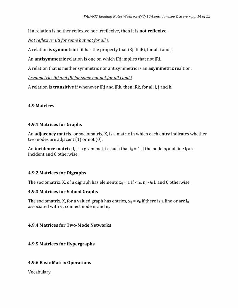
4.9 Matrices

4.9.1 Matrices for Graphs

An adjacency matrix, or sociomatrix, X, is a matrix in which each entry indicates whether two nodes are adjacent (1) or not (0).

An incidence matrix, I, is a g x m matrix, such that iij = 1 if the node ni and line lj are incident and 0 otherwise.

4.9.2 Matrices for Digraphs

The sociomatrix, X, of a digraph has elements xij = 1 if <ni, nj> ∈ L and 0 otherwise.

4.9.3 Matrices for Valued Graphs

The sociomatrix, X, for a valued graph has entries, xij = vk if there is a line or arc lk associated with vk connect node ni and nj.

4.9.4 Matrices for Two-Mode Networks

4.9.5 Matrices for Hypergraphs

4.9.6 Basic Matrix Operations

Vocabulary


The size of a matrix is the number rows and columns.

A square matrix is a matrix has the same number of rows and columns.

Each entry in a matrix is called a cell.

Symmetric matrix: xij = xji for all i, j.

Matrix Permutation

Transpose: interchanging the rows and columns of the original matrix.

Addition and Subtraction: summation/subtraction of the elements in the corresponding cells of the matrices.

Z = X+Y: zij = xij + yij

Z = X-Y: zij = xij - yij

Matrix Multiplication

Matrices X and Y have to be of the same size.

Z = YW: zij = ∑ yilwljℎ𝑙𝑙=1

The number of columns in Y must equal the number of the rows in W

Powers of a Matrix

.

Xp = the matrix product of X times itself, p times.

X has to be a square matrix

Boolean Matrix Multiplication

.

Z⨂ = X⨂Y: zij⨂ = 1 if ∑ 𝑦𝑦il𝑤𝑤lj > 0ℎ𝑙𝑙=1 ; zij⨂ = 0 if ∑ 𝑦𝑦il𝑤𝑤lj = 0ℎ

𝑙𝑙=1

4.9.7 Computing Simple Network Properties

Walks and Reachability

Entries of matrix X[∑] = X + X2 + X3 + … + Xg-1 , give the total number of walks from ni to nj.

None-zero elements of X[∑] indicate reachability.

Geodesics and Distance

Starting with p = 2, compute power of the matrix, X[p]. If xij[p-1] = 0 and xij[p] > 0, then there is a shortest path of length p between ni and nj.


Computing Nodal Degree

Incidence matrix: d(ni) = ∑ 𝐼𝐼ij𝑚𝑚𝑗𝑗=1 ,where m is the number of lines.

Sociomatrix: d(ni) = ∑ 𝑥𝑥ij𝑔𝑔𝑗𝑗=1 = ∑ 𝑥𝑥ij

𝑔𝑔𝑖𝑖=1 = xi+ = x+j

Digraph:

• dO(ni) = ∑ 𝑥𝑥ij𝑔𝑔𝑗𝑗=1 = xi+

• dI(ni) = ∑ 𝑥𝑥ji𝑔𝑔𝑗𝑗=1 = x+i

Computing Density

∆ = ∑ ∑ 𝑥𝑥ij

𝑔𝑔𝑗𝑗=1

𝑔𝑔𝑖𝑖=1

𝑔𝑔(𝑔𝑔 − 1)

4.10 Properties of Graphs, Relations, and Matrices

4.10.1 Reflexivity

A simple graph is irreflexive since no <ni, ni> are present. In corresponding sociomatrix of the graph, main diagonal are undefined.

If all loops are present, the graph represents a reflexive relation. Main diagonal of the sociomatrix, xii = 1 for all i.

If for some i but not all, values xii =1, then the graph represents a not reflexive relation.

4.10.2 Symmetry

A nondirectional relation is always symmetric.

In a directed graph symmetry means <ni, nj> ∈ L implies <nj, ni> ∈ L.

4.10.3 Transitivity

In order for the relation to be transitive, whenever xij[2] ≥ 1, then xij must equal 1.


Core discussion networks for Americans1

Purpose

• Descriptive overview of features of core social networks of Americans with network

concepts

Data source

• 1985 General Social Survey (GSS)

Sample: nationally representative sample of Americans; 1531 people

A first step toward establishing a standardized instrument to collect social

network data

Before 1985 GSS, the absence of standardized instruments for

collecting data complicated comparison, replication of findings, and

accumulation knowledge.

Operational definitions

• Names of alters matter!!

Name-eliciting device (name generator) sets operational boundaries on the

interpersonal environment

• So GSS used a name generator: “discuss important matters”

GSS asked each respondent about those persons with whom a respondent

“discuss important matters”

1 Marsden, Peter V. (1987). “Core Discussion Networks of Americans.” American Sociological Review, 52(2),

122-131.


But the definition of what was considered “important” was left to respondents;

intimacy or positive affect

Moderately intense content which represents a middle ground between

acquaintanceship and kinship

Less ambiguous in its meaning than friendship

Measures of the structure of interpersonal environments

• Individual attributes

Gender, race/ethnicity, education, age, and religious preference of each alters

• Social attributes

Respondents were asked to name all those people with whom they discussed

important matters within the past six months

All sub-questions focused on the first five names mentioned

GSS data presents data on the following three items:

Network size

• The number of alters

Network density

• Availability of social support

Potential strength of normative pressures toward conformity

Capacity of alters to collectively influence the respondent

• Unit of measure

1: especially close


0: total strangers

0.5: otherwise

Heterogeneity of alters

• Diversity of persons an individual can contact within his or her interpersonal

environment

• Four types of heterogeneity

Age and education

Quantitative variable

Measured as the standard deviations of alter characteristics

Race/ethnicity, and gender

Qualitative variable

Measured as the Index of Qualitative Variation (IOV)

The average American discussion network

• Univariate Distributions of Measures of Network Form and Composition


• Network Density, Heterogeneity, and Proportion Kin


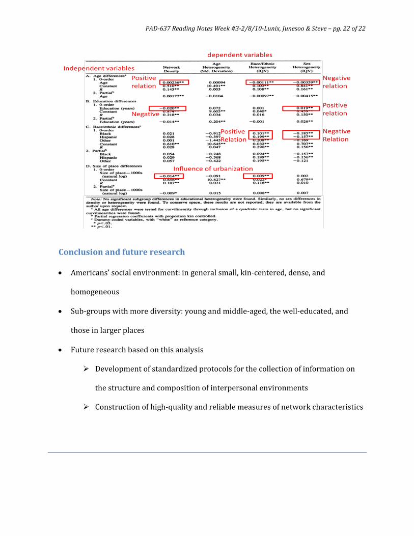
Subgroup differences in network form

• Subgroup Differences in Network Size and Kin/Nonkin Composition (Unstandardized Regression Coefficients)

• Subgroup Differences in Network Size and Kin/Nonkin Composition

(Unstandardized Regression Coefficients)


Conclusion and future research

• Americans’ social environment: in general small, kin-centered, dense, and

homogeneous

• Sub-groups with more diversity: young and middle-aged, the well-educated, and

those in larger places

• Future research based on this analysis

Development of standardized protocols for the collection of information on

the structure and composition of interpersonal environments

Construction of high-quality and reliable measures of network characteristics

Wasserman, S. & Faust, K. (1994). Social network analysis ... · PDF fileapplications. New...

Documents

Transcript of Wasserman, S. & Faust, K. (1994). Social network analysis ... · PDF fileapplications. New...