PB 82....; 147q?7

WASHINGTON UNIVERSITY

SCHOOL OF ENGINEERING AN C APPLIED SCIENCE

DEPARTMENT OF CIVIL ENGINEER1NG

SHORE - IV.

Finite Element Program for Dynamic and Static Analysis

of Shells of Revolution

USERS' MANUALby

O. M. El-Shafee, P. K. Basu, B. J. Lee

and

Research Report No. 56

P. L. Gould

Structural Division October 1981

This report is part of final report forNational Science Foundation Grant

PRF7900012

R'tPRODUC'tD B~

NATIONAL TECHNICALINfO~MATION SERVICE

us DfPAR1MENf Of COMMERCEStRINGfiElD VA 1216:

SHORE-IV

Finite Element Program For Dynamic&

Static Analysis of Shells of Revolution

USERS' HANUAL

by

O. M. El-Shafee, P. K. Basu, B. J. Lee

and

P. L. Gould

Research Report No. 56, Structural Division

Department of Civil Engineering

School of Engineering and Applied Science

Washington University

October 1981

Any opinions, findings, conclusionsor recommendations expressed in thispublication are those of the author(s)and do not necessarily reflect the viewsof the National Science Foundation.

PMF~E

The SHORE-IV program can be used for the static and dynamic analysis

of arbitrarily loaded thin elastic shells of revolution with or without

column supports, in the elastic regime. The soil effect on the dynamic

behaviour can be considered. This manual describes the procedure to be

followed in preparing the input data for this program and also assists

in the interpretation of the output. A number of sample inputs and

outputs utilizing the various options of the program are included. This

and the accompanying Theoretical Manual comprise the documentation of

SHORE-IV program.

, ,

1;'

TABLE OF CONTENTS

Section

Introduction " __ . til • 1

Input for SHORE-IV Program ••••••••••••••••••••••••••••••• 10

Card Formats

Data Cards for

............................. ................. ,. e- .

Each Problem ill •••••••••••••••••••

16

17

A.

B.

Problem Identification Card ••••••••••••••••••••••••

Problem Control Card ..••..••...•.•....•....•.•...•.

17

18

C. Element Cards . . 22

D. Nodal Point Cards . . 29

E. -

F.

Material Information Cards

Displacement Function Card . ..32

38

G.

H.

1.

Output Requirement Cards •••••••••••••••••••••••••••

Control Data Cards for Dynamic Analysis ••••••••••••

501.1 Cards .

39

45

48

J. Loading Information Cards • e- . 53

K. Data Cards for Dynamic Analysis by DirectIntegration " " _-# __ II .. .. • .. • .. .. .. .. .. .. .. .. .. .. .. • .. .. 58

L. Data Cards for Dynamic Analysis by ResponseSpec t r'lJJIl _ # .. .. .. .. • .. • .. .. .. .. .. .. • .. .. .. .. .. 63

M. Last Control Card .. " .. 66

SHORE-IV Program Output - '................ 67

Acknowledgements

Appendices

......................................... 0 .. 71

Appendix A

Appendix B

Appendix C

System Control Cards ••••••••••••••••••••••

Elements of Constitutive Matrix •••••••••••

Intermediate Printout Option Codes ••••••••

72

73

75

Appendix D - Direct Integration Scnemes

! f !

77

Table of Contents (cont.)

Section

Appendix E - Listing of 'FOHARM' ••••••••••••••••••••••• 83

AppendixF - List of 'THPLOT' •••••••••••••••••••••••••• 90

Appendix G - Demonstration Problems •••••••••••••••••••• 92

Example No. 1 - Free Vibration Analysis of aCylindrical Shell.................. 93

Example No. 2 - Free Vibration Analysis of aHemispherical Shell................ 95

Example No. 3 - Free Vibration Analysis of EmptyWater Tank with Soil InteractionEffect III • • • • • •• • • • • • • 97

Example No. 4 - Static Analysis of Column SupportedHyperboloidal Tower Under WindLoad ••....•.................•..•... 100

Example No. 5 - Dynamic Analysis of a Free-FixedCylindrical Shell Under BlastLoad .•..••••.••.•••. III ••••• III • • • • • • • • 103

Example No. 6 - Hyperboloidal Shell Under DynamicWind Load .........................• 106

Example No. 7 - Response Spectrum Analysis ofHyperboloidal Shell With SoilInteraction ~_~_.._~oo: -=-=-109 _

Example No. 8 - Time History Analysis of Hyper-boloidal Shell •.••••••••••••••••••• 113a. With Soil Effectb. Without Soil Effect

References •••••••••••••••••••••••••••••••••••••••••• fl· ••••

.IV

117

INTRODUCTION

The SHORE-IV program is designed for the linear static and dynamic

analysis of arbitrarily loaded thin to moderately thick elastic shells

of revolution. The meridional curve of the shell may have any quadratic

shape including the closed end case. The shell may be isotropic, or

single or multi-layer orthotropic, with the two principal material

directions at any point coinciding with the two principal directions of

the middle surface. The shell may have discrete supports in the form of

a framework of linear members with various end conditions and arrange-

ments. Such a framework may also be located at any other level except

at the top. Also, complete framed structures having the form of a

surface of revolution with the linear members running along the principal

directions of the middle surface can be analyzed. As a special case,

flat axisymmetric plates may also be considered.

Axisymmetric shells founded on footing foundations may be analyzed

dynamically including the soil-structure interaction effect. The soil

model consists of isoparametric quadratic solid axisymmetric elements

with transmitting_boundaries to account for the far-field effect. The

soil may be an elastic half-space or horizontally layered strata underlied

by bedrock at an actual or assumed depth. Cross-anisotropy for the soil

material is assumed. Element to element variation of material properties

is admissible. The user may supply detailed information for the soil

data or may supply only as few as three cards for the soil data, with

automatic data generation by the program. In the case of deep foundations--

the soil effect can not be considered.

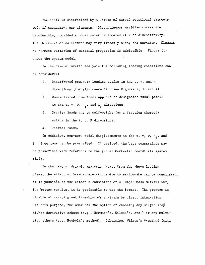
The shell is discretized by a series of curved rotational elements

and, -if necessary, cap elements. Discontinuous meridian curves are

permissible, provided a nodal point is located at such discontinuity.

The thickness of an element may vary linearly along the meridian. Element

to element variation of material properties is admissible. Figure (1)

shows the system model.

In the case of static analysis the following_loading conditions can

be considered:

1. Distributed pressure loading acting in the u, v, and w

directions (for sign convention see Figures 2, 3, and 4)

2. Concentrated line loads applied at designated nodal points

in the u, v, w, S~, and ~e directions.

3. Gravity loads due to self-weight (or a fraction thereof)

acting in the Z, or R directions.

4. Thermal loads.

In addition, non-zero nodal displacements in the u, v, w, S~, and

Sa directions can be prescribed. If desired, the base constraints may

be prescribed with reference to the global Cartesian coordinate system

(R,Z).

In the case of dynamic analysis, apart from the above loading

cases, the effect of base accelerations due to earthquake can be considered.

It is possible to use either a consistent or a lumped mass matrix; but,

for better results, it is preferable to use the former. The program is

capable of carrying out time-history analysis by direct integration.

For this purpose, the user has the option of choosing any single step

higher derivative scheme (e.g., Newmark's, Wilson's, etc.) or any multi­

step scheme (e.g. Houbolt's method). Otherwise, Wilson's a-method (with

-3-

AXIS OF SYM.

r---------

r------Ir------

REGION MOOEL

A HPRS" ELEMeNTS

HPRS ELEMENTS

APPROACH

CONTINUOUS BOUNDARY

SUPCRPOSlTlON

,-------c OPEN ELEMENT SUPERPOSITION

1-------SUPERPOSITIONBOUNDARY ELE­

MENT

E EQUIVALENT aOUN- CONTINUOUS BOUNDARYDARY SYSTEM

o

" HPRS ::. High- Precision Relational Shell

RING FOOTING

SOIL MEDIUM

COLUMNS

Q

u

t

L~-------I

T- ~ ------ ----c:Q I- _LQ.W!B ....!:J.N.lEL _ --

+

Tw

--L

Figure 1. Proposed Model for _aCooling Tower Shell

Ne

-4-

a~

Stress Resultants

Stress-Couple Resultants

Figure 2. ,Sign Conventions

Qt1l

hn ~ THICKNESS

hk - THICKNESSho - THICKNESS

MIDDLe· SURFACE

OF OUTER LAYER

OF INTERMEDIATE LAYER

OF MlOOl£ LAYER

Figure 3. Multilayer Shell Element

-6-

\~

\

END DISPLACEMENTS

END FORCES

Figure 4. Sign Convention for Members in Open Type Elements

e = 1.4) can be used as the default option. If desired, it is possible

to specify more than one time step. This may sometimes be helpful in

saving computer time. Earthquake analysis can also be carried out by

the response spectrum method. The free vibration analysis is carried

out by the combined Sturm sequence and inverse iteration technique [1].

All loads~hich are not axisymmetric are required to be expanded

in Fourier harmonics; for this purpose, a separate program package

(FOHARM) may be used. The loading need not be symmetric about the

e = 0° line, i.e. both sine and cosine harmonics can be considered

simultaneously. The number of harmonics to be considered will depend

upon the nature of the loading and the accuracy desired. The distributed

loadings and the temperature distribution may vary linearly along the

meridian of each element.

The input data format is such that repetitive data is reduced to

minimum. Moreover, in the event of some specific errors in input data,

the run is terminated before the problem is executed and the corresponding

error code, or message is printed out.

Various printout options for displacements, stress-resultants and

stresses are available. The time history plot for displacements and

stress resultants can be obtained on the printer. Alternatively, for

offline plotting on a 760/563 Calcomp plotter system, a plot tape can

be created. Also, the time history results can be obtained on punched

cards for further uses.

This program is an extension of the Shell of Revolution Finite

Element Program SHORE-III [2,3]. It is written in FORTRAN IV language

and has been developed on an IBM 360/65 computer.

-0-

SHORE-IV is an in-core solver requiring less than 500 K in high

speed storage. For running the program it is necessary to use the

overlay structure shown in Figure 5.

The input data and intermediate results are required to be stored

on seventeen scratch disk files and three tapes. For Calcomp plotting a

800 bpi, 9-track tape is also required.

-Ij-

ROOT SEGMENT (300 K)

MAIIlCAPTOESUGoGl-lPROOGN'I'RA

OMINVrPR2IPRSLASHPRINTSOLV

STOTSTRESSZEROSCPlrrIJ.t*DATE"

I I I lOVERLAY a

l OVERLAY as OVERLAY as OVERLAY a, OVERLAYag

OYR2

DATAl EASt

LISTED CARS SSGPR EIGSNS

SETFC OISM INVtT

SETPC SNCO OYR; ISOLAT

ZERO1 GUIX NtlMBURZER04

OVERLAYa2

OVERLAYa4 OVERLAYa6 OVERLAY as

alOE STATICSSS CALQFEIG/II oATA2 ZER03 asGPEIG/ST SMATS oATA3EL.\tiT IPRS OYRIFACT RFt'N MSTFAR S'lORS PLHtSFeT 7ER02 SST!iN1CL i'IIIISlNVLYRSSSTSUBASE

I IOVERLAY 8

1OVERLAY 8

2OVERLAY Y

lOVERLAY Y2

PRPLOT

ARC eLSl LOAD BLOT CCl'torCALC CLB2 !'MROo AXIS'CALGS CLOI PROD ear LIN!!"CALH eLD2 TASL NUMBER"CALlIC CLAM TABLe SSOT PLOT*CALP CLBf~ TABLFP PLOTS'eAPl CLoM TEMP SCALS"eLAI FINA ZER02 SYMBOL"

CLA2 !'MINA

IIOTE: Subt'Outines Marke<l with an Asterisk C'J areInstallation Dependent.

Figure 5" Overlay Structure of SHORE-IV

-.lU-

INPUT FOR SHORE-IV PROGRAM

The input data for the SHORE-IV program consists of complete data

sets for each problem to be run, placed sequentially. The data for each

problem is organized into a number of groups associated with card types

A through L. Some of these groups, namely those corresponding to card

types E, G, H, etc., are subdivided into various optional blocks of

input data. There is no limit to the number of problems that can be

executed per run. The schematics of input data decks for various types

of problems are shown in Figures 6 to 10.

The program uses seventeen temporary disk files, namely 9, 10, 11,

25, and three temporary tapes, namely 26, 27 and 28. In the case of

dynamic analysis when Calcomp plotting of time history response is

desired, a permanent tape, the PLOTTAPE, (9 track, 800 bpi), is required.

Therefore, the above mentioned deck should be preceded by suitable

system control cards allocating the above mentioned spaces. For example,

on an IBM 360/65 computing system, the JCL statements shown in Appendix A

may be used.

-11:-

(~JOBEND

/® PROBLEM IDENTIFICATION CARD:I . PRCB. 3

PROBLEM IDENTlACATlON CARD:PROB. 2

( ® PROBLEM IDENTIFICATION .CARD:PROB. I .

(JCL CARDS ASSIGNING SCRATCH

DISK AND TAPE SPACE

(' EXEe CARD

SYSTEMS JOB CARD

-

.,1

-

Figure 6·. Input Data Stream for So Job

(CD

~DJNG

INFO

RM

.trrK

»JC

ARD

S(n

eede

dfo

rea

chha

rmoo

/cl

.

('®

OU

TPU

TR

EQU

IREM

ENT

CARD

S

,/®

DIS

PLAC

EMEN

TFU

NC

TnJ

CARD

(CP

T)

('<6)

MA

TER

IAL

INFO

RM

ATIO

NC

ARD

S

~~

,/@N

OD

ALPO

INT

CAR

DS

E:RM

(©E

LEM

EN

TC

ARD

S~'CIRCUIrlFEJ

OU

TPU

TC

(@PR

OBL

EMCO

NTR

OL

CARD

-®

PR

OB

LEM

ICE

-lTIF

ICA

TIO

NC

ARD

f--

.....-

--

ISPl

.AC

EMEN

TC

ARD

S(O

p'/OI

I1'11

JTH

ER

MA

l.I.O

ADIN

OC

ARD

(opt

lono

l)EN

TRAT

EOtJ

OO

ALC

IRC

LEG

CA

RD

S(o

ptiO

llO/}

·RJB

IJTED

LOAD

ING

CARD

S(o

pt/(,

Jlol

)'N

TRO

LCA

RDCA

RD INTE

:DO

UT

CA

RD

S{O

flIio

tId'

OC

AT

'ON

CARC

IS(o

plio

lao/

JAR

O.

I I-'

N I

Fig

ure

7.

Inp

ut

Dat

aD

eck

for

Sta

tic

An

aly

sis

I l­ v I

ftO

Alm

GCX

WTR

OI.

CARD

~TI

TLE

CARD

'AA'

TOUT

CA.

qo(o

p/Q

nQ/'·

CAR

D

ItW

EA

NA

U'S

ISCA

RD1T

Rf)(

CARD

(0I...

OADN

GIN

FORM

ATIC

1'JCA

RDS

(nee

ded

for

each

horm

oolc

J

(CD

$O

U...

'.iC

ARD

S

(<8>

CO

NTR

OL

DATA

CAR

DS

FOR

DYN

AMIC

ANAL

YSIS

('®

OU

TPU

TR

EQU

IREM

ENT

CAR

DS

r--

('®

DISP

LACE

~IEN

TFU

NC

TIO

NC

NID

(CP

r)

,/®

MAT

ERIA

LIN

FORM

ATIC

NC

ARD

S-

~-AG

(@N

OD

ALPO

INT

CAR

DS

-A"E

RMt!l

/Al

(©E

LEM

EN

TC

ARD

S_

PUT

CON'

(®PR

OBL

EMC

ON

TRO

L·CA

RDr-

-

,@

PRO

BLEM

IDEN

TIFI

CAT

ION

CAR

Dr--

----

r--

Fig

ure

8.

Inp

ut

Dat

aD

eck

for

Fre

eV

ibra

tio

nA

nal

ysi

s

CAllO

S(o

pIfa

tal)

l'"r'f

£C

ARD

lYSI

SCA

RDo

.AiiA

aNG

CONT

ROl.

CARD

AciA

DTI

TLE

CARD

:l.P

J::C

;{K

Al"

VA

LlI

&:

....

."..

...'~

.S

Pf,"

Clli

AL

OAM

PIN

O-R

-C.T

10C

ARO

SC

ON

TRa.

.C

ARD

FOR

RE

SF(

WS

ESP

ECTR

UM

..:J:.PONS~i~CR~~'

~~

TITL

EC

ARD

(©DA

TAC

ARD

Sro

om

'NA

MIC

ANAL

YSIS

BYR

ESPO

NSE

SPEC

TRU

M

(Q)

LOAD

ING

INFO

RM

ATIO

NC

ARD

S

('ID

SO

ILC

ARD

S

(®C

ON

TRO

LDA

TAC

ARD

SFO

RD

YN

AM

ICA

NA

LYS

ISr--

(@O

UTP

UT

RE

QJI

RE

ME

NT

CAR

DS

A:(®

CYS

PLAC

EMEN

TAJ

NC

TIO

NCA

RDIO

Pr)

-('

®M

ATE

RIA

LIN

FOR

MAT

ION

CAR

DS

= ~YNAMIC

LOA

!

(@N

OD

ALP

OIN

TC

ARD

SI--

lGEN

VAl.U

£A

Joj

ASS

MA

mlX

CI

(©E

LEM

EN

TC

AR

DS

~MEOIATE

PRW

TOlJT

r--

TPU

TC

CN

TRO

LC

ARD

("@

PRO

BLEM

CC

WTR

OL

CAR

DI-

®P

RO

BLE

MID

EN

TIFI

CA

TIO

NCA

RD---

f-

-I--

Fig

ure

9.

Inp

ut

Dat

aD

eck

:fo

rR

esp

on

seS

pec

tru

mA

nal

ysi

s

.RE

CO

RD

PO

INT

CA

RD

S~

-TIn

.1!

CARD

FOR

INPU

TTI

ME

fUN

CTI

ON

IHTT

W.

COND

lTIC

WC

ON

lnO

LCA

RD.

_£lA

TACC

WTR

OL

CARD

FOR

DYN

AMiC

ANAI

YSJS

.®

DATA

.CAR

DSFO

RfJ

r'NAM

ICD

IRE

CT

INTE

GR

ATED

SCH

EME

CAR

D,A

NA

LY

SIS

BYDI

RECT

INTE

GRA

TIO

N

tDW

ADIN

GIN

FOR

MAT

ION

CAR

DS

I

(nee

ded

for

each

harm

onic

)

('CD

.SO

ILC

ARD

S

/(fp

CO

NT

RO

L-U

4TA

CARD

SFO

Rr

-D

YNAM

ICAN

ALYS

IS

®CX

JTFU

TR

EQU

IREM

ENT

CARD

S

®aS

PLA

CE

ME

NT

FUN

CTI

ON

CARD

((F

'f)

(®M

ATER

IAL

INFO

RM

ATIO

NCA

RDS

(@N

OD

ALPO

If-v'T

CAR

DS

('©

ELEM

ENT

CAR

DS

(®PR

OBL

EMCO

NTRO

LC

ARD

®P

RO

BLE

MID

ENTI

FIC

ATIO

NC

ARD

I--

I--

I--

I--

I--

ISPl

..AC

EMEN

TC

ARD

S(o

ptlo

ndl

rHE

RM

.U.

LOA

DIN

GCA

RPS

(opt

IOllQ

I)Iml--.<~~ENTRATED

NO

DAl

.C

lRC

I.EIN

GCA

ROO

(opl

iallJ

l1•

ISTR

IBU

TIO

NLO

ADIN

GC

ARD

S(q

tlon

all

OAD

lNG

CO

Nnl

OL

CARD

ADrrn

.£C~D

~.N4MJC

LOA

DTY

PEC

ARD

..~E:

::::EE::

~D/'r

iME"

'HlS

TOR

fW

TPU

TC

ON

TRC

1,C

ARD

'CIRNJu~~~1.

~<XffcwCAROcJo~o1~~J.ct,

t--'

"---

A2l

.!T

PlJ

TC

ON

TRO

LC

ARD

I t­ l.. I

Not

e:C

ards

mar

ked

wit

han

ast

eri

sk(*

)m

ayb

ere

pea

ted

for

each

harm

onic

depe

ndin

gup

onth

eo

pti

on

CO

desp

ecif

ied

inpr

oble

mco

ntr

olcard~

Fig

ure

10

.In

pu

tD

ata

Dec

kfo

rT

ime

His

tory

An

aly

sis

by

Dir

ect

Inte

gra

tio

n

-.16-

Card Formats

'The integer field is expressed as I2, I3, IS, etc., meaning thereby

. integer fields of 2, 3, 5, etc. characters. The floating point numbers

are indicated mostly by F8, F9, FlO, etc., meaning floating point num-

bers with fields of 8, 9, 10, etc. characters. In a few cases the

floating point numbers are expressed as E9, ElO, meaning floating

point numbers with exponents consisting of 9, 10 characters • Floating~.-. . . -

point ..number~...shal1..be entered with a decimal po.int, and those in E- .

format..and the.inte.gersmust be right justified. For each record (or

card) of 80 columns, the formats shall be as stated in subsequent sections.

Units

Any consistent units may be used. Of course, the force and distance

units for all input quantities should be the same. For convenience the

units used may be stated on any of the title cards.

-17-

i)A1'A CARDS FOR EACH PROBLEM

A. - Problem Identification Card:

The information contained on this card is the first_ print out for

each problem and is usually the title assigned to the problem. In- the

last eight columns of this card the code words for input data echo op-

tions are stated.

Columns

2 - 72

73 -79

Format

A

A

Entry

Problem Title to be output withresults

NO' ECHO - if the problem is to berun without printing the echo ofinput data

If the columns 73 - 80 are left blank the input data echo is printed

and also the problem is run.

-llS-

B. Problem Control Card:

The information contained on this card is as follows:

1. The number of rotational finite elements used for discretizing

the structure. The maximum number of elements allow~d·i~ 48.

2. The number of harmonic loading cases to be considered.

3. the type of structuralcro~s-sectionwith the following

code numbers:

isotropic

single layer orthotropic

framed

multilayer(Each layer may beorthotropic orisotropic. )

o (at' blank)

1

2

number of layers {must beodd} • The minimum is 3 andmaximum 7.

In the case of multilayer shells,. even if the number of layers is

not odd and!or the layeTs are unsymmetrical, the problem can be

solved to a point by specifying 2 as the code ulJmber; the output

results will be stress resultants and displacements only.

4. The code number for the type of analysis:

static analysis 0

free vibration analysis 1

time history analysis

mode superposition

response spectrum

direct integration

2

3

4

5. The maximum degree of polynomial approximation to be used in

the stiffness and mass matrices. The maximum is 6, and the

default value is 3. It is recommended that 6 be used for

static analysis and 3 for dynamic analysis [3].

6. The code number to avoid inputing of repetitive data required

for the time history analysis by direct integration:

Control data for dynamic analysis,or time history data to be suppliedfor each harmonic

The above data to be supplied forthe first harmonic only

The format of Problem Control Card will be as follows:

1

°Columns

1 - 5

6 - 10

11 - 15

16 - 20

21 - 25

30 - 35

36 - 40

41 - 45

Format

15

IS

15

IS

15

15

15

15

Number of finite elements to be used

Number of harmonic loading cases

Relevant code number for shell material

Code number for type of analysis

Maximum degree of polynomial approximation

1 or 0, refers to control data fordynamic analysis by direct integration

I or 0, refers to time history data

1 or 0, refers to soil-structure inter­action effect

The flag 1 in the sixth field signifies that the control data card

for dynamic analysis, J(b), is input separately for each harmonic. If

left blank, it signifies that this card is input for the first harmonic

only. Similarly, the flag 1 in the seventh field signifies that the

input time function cards, J(e) and J(f), are input separately for each

harmonic. Otherwise, the same are input for the first harmonic only.

-20-

If the columns 41 to 45 are left blank the soil-structure interaction

is not considered.

If the flag 1 appears in the column 45 the interaction effect is

considered and the soil data of section "I" must be supplied.

For static analysis columns 41 to 45 must always be left blank.

C. Element. Cards

One card is required for each element, with the cards placed in

numerical sequence of element numbers. The elements are, required

t.o be numbered consecutively from the top to the bottom of the shell

beginning with element number- 1. Flat plates should be numbered

consecutively from inside to outside. Only one cap element may be

used for the analysis of a closed shell of revolution and this must

be numbered element 1. (See Figures 11 and 12 ) •

If some cards are: omitted~ the element information for the omitted

elements is set equal to the element information on the preceding ele­

ment card. However, element cards for the first and~ elements must

always be supplied.

Each element card should state the element number, the element type,

the meridian definition cnde and certain constants defining the meridian.

For element types, refer to the library of elements' in P,ij;U:t"O 13. In the

case of open type elements, the element type field also states the num­

ber and end conditions of the members comprising the open type element.

For end conditions of open type elements, refer to ,Figure 14. The

meridian definition code defines how the. meridian curve. of the. element

is specified. Far a- global coordinate system the code number is zero (or

blank) and for c,.local coordinate systelll it is the nodal point number where

Z • o. For 'a. type. 2 cap element, the Z-coordinateof the pole must be

zero. The meridian definition code is not appll.cabla in the case of. . .. ",.,

type 4 and type 5 elements.

'aEMENT- NUM.BER. •

TOP

.-- AXIS OF. REVOLUTION

OPEN

W - Ncrmal dis.pla.c~~

.84> - Rotoikif in 4> - direction

138 - Rofation in 8 - direction

U - Displacement in eII- direction

V - Displacement in e- qirectfon

CLO$ED TOP

P t---- -,~

, InJ);)}IIIIIIIIIIIlI

R•

Figure 11. Finite Element Discretization of Shell of Revolution

E~MENT 1YPE 4

£LEMENT " TYPE. P

//

//

/

-"", ......"- .......

""'\. .\\

\\\\

6 .NODAL .PO,~rNUMBER

----Ri{=R3

RFtf(=R4} ., .'

....­.,;'

.//

//

//

I

\\\\

\

·ELEMENt!"NUMBER'

Figure 12. Finite Element Discretization of an Axisymmetric Plate

-:L4-

CODE TYPE· SHAPE

"GENERAL,/

I-- fI (CURVED)

II

\,

CAP ~Z ( lNF1NlTE ,/

SLOPE) /I

CAp: /3 ( FINITE ,/

"SLOPE) .I

,~

CAP /I

I4 (FLAT I

PLATE)

if

GENERAL,/

5(FLAT /

,,'PLATE) "

It

Figure 13. Library of Elements

CCDE ·TYPE

6 OPEN

7 OPEN

8 OPEN

9 OPEN

SHAPE

Figure 13. (Contd.)

FUll. CONTINUITY ATBOTH ENDS

CODE NUMBER: I

MEMBERS MONOLITHiCPINNED ENDS

CGeE NUMBER:2

MEMBERS AND ENDSPINNED

CODE NUMBER: 3

TOP CNDS LJXE CODE NO.1

BOT. ENOS LIKE CODE N03CODE NUMBER:4

TOP ENDS LIKE CODE na2BOT. €NDS LIKE CODE NO~3

CODE NUMBER:5

TOP ENDS, LIKE CODE NO.3BOT. ENDS UK£. CODE NO.1CODE NUMBER: 5

TOP ENDS LIKE c CODZ NO.3Bor . ENDS LIKE CODE N02CODE NU'AB£R: 7

Figure 14. End Conditions of Open Type Elements

-1./-

In the case of element types 1 to 3, the constants are actually the

six coefficients of the following equation of the meridian curve~

in which

AZ2 + BRZ + CR.2 + DZ + ER + F o

Rand Z are the coordinate defining points on the meridian (see

Figure 11); and A, B, C, D, E, and F are constants for the meridian curve

with the requirement that C should always be positive. In the case of ele-

ment types 4 and 5, it is required to specify the coefficients A and B

only, A being equal to the R-lo~ation of nodal point i,and B equal to ~e

R-location of nodal point (i+1), as shown in Figure 12. IIi the case

of element types 6 to 9, with the theoretical middle surface following

the shape of t:1:e frustum of a' cone, it is necessary to specify the

coefficients D, E, and F only.

The format of Element Cards will be as follows:

Columns Format Entry

1 - 3 I3 Element number

4 - 10 I7 Element type (in the case ofop~n typ~ elements see next page)

11 - 13 I3 Meridian definition code

14 - 24 Fll A coefficient

25 - 35 F11 B coefficient

36 - 46 Fll C coefficient

47 - 57 F11 D coefficient

58 - 68 Fll E coefficient

69 - 79 F11 F coefficient

-:w-

In the case of open type elements the entry in Columns 4 to·10

shall be

Columns Format:. Entry

4 - 8 1.5 Number of members in the element.

9 11 Code number for end conditions (seeFigu-re 1.4)

10 11 Element type

-29-

D. Nodal Point Cards

One card is requi.red for each nodal point, placed in numerical se­

quence of nodal numbers. Nodal points must be numbered consecutively'

from the top to the bottom of a shell, or from the innermost part to

the outer part of a plate, beginning with nodal point number 1 (see

Figures 11, 12).

If some cards ar~ omitted" the omitted nodal, points are generated at

equal intervals between the defined nodal points. However, nodal point

cards for the first and~ nodal points must always be supplied.

Each nodal point card states the nodal point number, Z-coordinate

of the nodal point in global coordinate system and the geometric con-

straints corresponding to the displacement components u, v, w, S$' and

Sa at the nodal po~nt. When a displacement component is zero, the con­

straint code number corresponding to that displacement component will be

1. When a non-zero displacement component is specified, the constraint

code number will be 2. If, however, the displacement component is not

constraine~ the code number will be zero (or blank). Constraint codes

for all omitted nodal point cards are set equal to zero. Thus, it is

necessary to provide data for all ~onstrained nodal points. The maximum

number of prescribed non-zero. constraints is limited to 10.

The format of Nodal Point Cards will be as follows:

Columns Format Entry

1 - 5 IS Nodal point number

6 15 FlO Nodal point location (Z-c90rdinatein global coordinate system)

16 - 20 IS Constraint Code for u-displacement

FIXED BASE(u =0,v=O,w=O,Pep=O,,8e=O)

TANGENTIALLY PINNED BASE

(u=O,v=O,w=O,!3e =0)

-30-

RADIALLY PINNED BASE(u=O, v=O,w=o,PcjJ=O)

FULLY PINNED BASE

(u=O v=O w=O). , )

Figure 15. Support Constraints for Open Type Elements

Columns Format

Zl - 25 IS

26 - 30 IS

31 - 35 IS

36 - 40 I5

4~ - 45 IS

-j.L-

Constraint Code for v-displacement

Constraint Code for w-displacement

Constraint Code for S~-rotation

Constraint Code for Sa-rotation

Blank or 1, the former signify thatthe support constraints refer to thecurvilinear reference frame and thelater signifies that the same referto the global cartesian reference frame

For the case of open type elements the suppor1;= constraints for various

Cnd conditions are shoTNU in Figure 15.

E. Materi~ Information Cards:

In the case of isotropic material, only one material info!'I!lation

car~ placed in nume~cal sequence of element numbers, is required for

each element. If some cards are omitted, the material information

for the omitted elements are set equal to those on the preceding card.

However mate~al infonnation cards for the first and~ eletnents

must be supplied. Each materlalinformation card states the eletllent

number, thickness of element, modulus of elasticity, Poisson's ratio,

shear factor, and mass density for the element. !n the case of open

tyPe elements, each material information card states the cross-

sectional area, torsional constant (Saint-Venant 1 s), modulus of

elasticity, moments of inertia about the circumferential and normal axes,

mass density, width and depth of the typical melllber, and Poisson t s

ratio. (.SQQ 'Figure. °16)

The format of Mater~al !nformat~on Cards for isotroEic material will

be a.s follows:

ColU1ml

1 - 3

4 - 12

13 - 21

22 - 30

31 - 39

40 - 48

49 - 57

F01:'mat

13

E9

E9

E9

E9

E9

E9

EntEZ

Element number

~~,kness of element at node. with snaller no:

'thickness of element at nQde with lUger no­(hi+l)

Modulus of elasticity.f'

!'oisson r s ratio

Shear factor (default ~ 5/6)

Mass dens ity of material

The format of Matertal Information Cards for o'Oen t!f!e elements

will be as follows:

-33-

SHELL

NODAL CIRCLE 'i+\' 'c::::::==::1

'-----MEMBER OF OPENTYf'E ELEMENT

Figure 16.

-j.4-

Cross-sectional area of member

Moment of inertia about the normal axis

Element numb er

+ I )z

For wind effectFor cols. effect

on the shellFor temp. levels

Width of member (be)

Mass density of material (Y/g)

Torsional constant (10 = I

Modulus of elasticity

Moment of inertia about thecircumferential axis

Column Format

1 - 3 13

4 - 12 E9

13- 21 E9

22 - 30 E9

31 - 39 E9

40 48 E9

49 - 57 E9

58 - 66 E9

67 - 75 E9 Depth of member (d )c

76 - 80 F5 Poisson's ratio

Note: Maximum number of different values for Poisson's ratio for open-

type elements is 16.

In the case of single layer orthotropic or multi-layer materials

or framed structures, a set of three material information cards are

required for each element, placed in numerical sequence of element

numbers. If such card sets are omitted, the material information for

the omitted elements are set equal to those on the preceding set.

However, material property cards for the first and last elements must

always be supplied. In this case, the first material information card

for each element contains the element number, and thickness of element.

The second and third cards contain.the te~ elements of the constLtutive

matrix [C], Appendix B.

Format Entry

FlO CnFlO C12

FlO C22

FlO C33

FlO C44

FlO C45

FlO C55

FlO C66

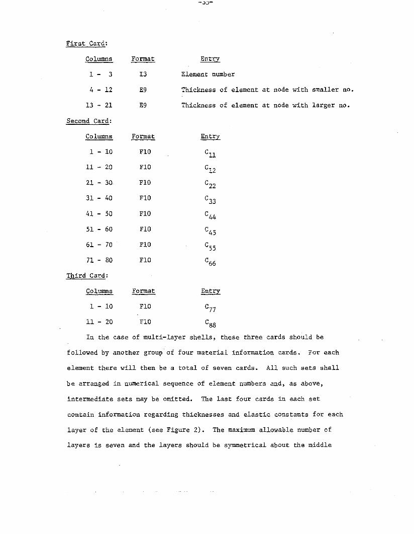
First Card:

Columns

1 - 3

4 - 12

13- 21

Second Card:

Columns

1 - 10

11- 20

21 - 30

31 - 40

41 - 50

51 - 60

61 - 70

71- 80

Third Card:

Columns

1 - 10

11 - 20

Format

13

E9

E9

Format

FlO

FlO

~

Element number

Thickness of element at node with smaller no.

Thickness of element at node with larger no.

In the case of multi-layer shells, these three cards should be

followed by another group of four material information cards. For each

element there will then be a total of seven cards. All such sets shall

be arranged in numerical sequence of element numbers and, as above,

intermediate sets may be omitted. The last four cards in each set

contain information regarding thicknesses and elastic constants for each

layer of the element (see Figure 2). The maximum allowable number of

layers is seven and the layers should be sYmmetrical about the middle

-.Jv-

surface in all respects. It may, however, be noted that if the number of

layers is even and/or the layers are unsymmetrical, the last four cards

in the set need not be provided since stresses cannot be computed.

The format of the additional sets of Material Information Cards for

multilayer materials will be as follows:

Fourth Card:

Columns

1 - 5

6 - 15

16 - 25

26 - 35

36 - 45

Fifth Card:

Columns

1 - 5

6 - 15

16 - 25

26 - 35

36 - 45

Sixth Card:

Columns

1 - 5

6 15

16 - 25

26 - 35

36 - 45

Format

IS

FlO

FlO

FlO

FlO

Format

FlO

FlO

FlO

FlO

Format

FlO

FlO

FlO

FlO

Element number

Thickness of middle layer (h )o

Thickness of layer next to middle (hI)'i.e. the outermost layer of a threelayer system

Thickness of layer next to hl(hZ)' i.e.the outermost layer of a five layer system

Thickness of layer next to h2 (h3), i.e.the outermost layer of a seven layer system

To be left blank

Modulus of elasticity in meridionaldirection (E~) for middle layer

- do - for layer '1'

- do - for layer '2'

- go - for layer '3'

To be left blank

Modulus of elasticity in circumferentialdirection (Ee) for middle layer

- do - for layer '1'

- do - for layer 'z'

- do - for layer '3'

-37-

Seventh Card:

Columns

1 - 5

6 - 15

16 - 25

26 - 35

36 - 45

Format

FlO

FlO

FlO

FlO

Entry

To be left blank.

Tangential shear modulus (G~e)for middle layer

- do - for layer '1'

- do - for layer '2'

- do - for layer '3'

When the number 0 f layers is threa, the· last two entries in each

of the above four cards should be left blank.. Similarly, in the case

of five layers the last entry in each of these cards should be left.

blank..

F. Displacement Function Card:

~ this card if columns 21-25 of the Problem Control Card are left

blank. For static analysis, it is recommended that 6 be used in each field

from columns 1-25. At the present time, it is recommended that the default

value be used for dynamic analysis [4]. Then, this card is not required., -

Otherwise, the degree of p~lynomial approximation for the displacement

functions to be used in forming the stiffness matrix (col. 1-25) and the

mass matrices (col. 26-50) may be specified shown below. However, the maxi-

mum permissible degree is 6. In the case of static analysis the columns 26

to 50 relating to the mass matrix should be left blank.

Column Format Entry

1 - 5 I5 Degree of polynomial approximationfor u

6 - 10 15 Degree of polynomial approximationfor v

11 - 15 IS Degree of polynomial approximationfor w

16 - 20 15 Degree of polynomial approximationfor e~

21 - 25 15 Degree of polynomial approximationfor Sa

26 - 30 15 Degree of polynomial approximationfor u

31 - 35 I5 Degree of polynomial approximationfor v

36 - 40 IS Degree-of polynomial approximationfor w

41 - 45 15 Degree of polynomial approximationfor Slj>

46 - 50 IS Degree of polynomial approximationfor aa

-39-

G. Output Requirement Cards:

a) Tne first card, the 'output control card', states the number of

circumferential locations where displacements, stresses, etc. in each

element are desired to be printed out, and also the number of inter-

mediate printout options desired. For available options see Appendix C.

The third field in this card represents the number of intermediate

stations within each element at which it is desired to compute displace-

ments and stresses. The default number is 5 and maximum is 9. The

fourth field states the number of modes to be considered in the case of

time history analysis by modal superposition (analysis type 2) or response

spectrum analysis (analysis type 3) and the sixth field indicates if it

is necessary to print out the input time history data for each time step

or the input response spectrum data. The seventh field to the sixteenth

field indicates the nodal points for detailed output and the corresponding

circumferential angle step for each node.

It should be noted that further output control information is

specified on the 'Loading Control Card', which is described later.

The format of Output Control Card will be as follows:

Columns

1 - 5

6 - 10

11 - 15

16 - 20

21 - 25

Format

IS

IS

IS

IS

IS

Number of circumferential locations wheredisplacements, stresses, etc. are desired(Maximum = 16)

Number of intermediate printout code numbersspecified (Maximum = 8)

Number of intermediate stations per elementwhere displacements, stresses, etc. aredesired (Maximum = 9; Default = 5)

1, if eigenvalues and eigenvectors arenot to be output; otherwise leave blank

Number of modes to be considered in analysistypes 2 and 3

Columns Format ~

26 - 30 15 1, if input time history, or responsespectrum data are to be printed out;otherwise leave blank

31 - 32 12 Node number at which detailed output isrequired (1st detailed node)

33 - 40 F8 Angle step for this node

41 42 12 Node number at which detailed output isrequired (2nd detailed node)

43 - 50 F8 Angle step for this node

71-72

73 - 80

12

F8

Node number at which detailed output isrequired (5th detailed node)

Angle step for this node

Note: Maximum number of nodes for detailed output is five.

The "Output Control Card" should be followed by "the nodal thickness

card" if columns 31 -+ 80 are not blank.

The format of the nodal thickness card shall be as follows: (5FIO.0)

Columns Format Entry

1 - 10 no Thickness of 1st detailed node

11- 20 FlO Thickness of 2nd detailed node

21 - 30 FlO Thickness of 3rd detailed node

31 - 40 FlO Thickness of 4th detailed node

41 - 50 flO Thickness of 5th detailed node

51 - 60 flO Last circumferential location at whichdetailed output is required (default = 180°)

If the first field of the output control card is not left blank,

the above card (cards) should be followed by the stated number of

circumferential location cards, one card for each location stating the

-4.L-

circumferential location (in degrees) where displacements, stresses,

etc., are to be output. The maximum number of locations is 16. If,

however, the first field of the output control card is left blank, no

circumferential location cards are required and results are output for

the location = 0° only.

If the second field in the output control card is not blank, the

circumferential location cards (if any) should be followed by the stated

number of intermediate printout option code cards, one card for each

option code. There are eight option code numbers, namely 86 to 93. For

a description of intermediate printouts corresponding to these option

codes, see Appendix C. If, however, columns 6 - 10 in the output control

card are left blank, no intermediate printout option code cards are

required.

The format of Circumferential Location Cards shall be as follows:

Columns

1 - 10

Format

FlO

Entry

Circumferential location in degrees

The format of Intermediate Printout Option Cards shall be as follows:

Columns Format Entry

1 - 5 15 Intermediate printout option code

b) In the case of time history analysis only, i.e. analysis types

2 and 4, one or more of the following cards are necessary. The first

card is called the 'time history output control card'. This card

states both the form and the extent of output desired. Any subsequent

cards are necessary only if the plotting option is utilized. It-is

possible to plot the displacement history, the stress resultant history

and the acceleration history. The maximum number of components allowed

for each case is ten. The response due to any number of harmonics be-

ginning with the first may be plotted. At the end~the sum total results

of all the stated harmonics at e - 00 are plotted. Flots can be obtained

either on the line prineer or off-line us:ing a 760/563 Calcomp Plotter System.

The format of Time History Output Control Card will be as follows:

Columns

1 - 5

6 - 10

11-13

16 - 20

21 - 25

26 - 30

31 - 35

36 - 40

41 - 45

46 - 50

Format

IS

IS

15

IS

15

15

I5

IS

IS

1~ if absolute maximum displacementsare to be printed; otherwise leaveblank.

1, if maximum displacements are tobe printed (at given time step' ,inte~u); otherwise leave blank..

l~ if displacements are to be printedat given time step interval; otherwiseleave blank:

The number of displacement compo­nents for which time histories areto be plotted (Maximum • 10).

1, if absolute maximum stress resul­t~ts are to be printed; otherwiseleave· blank.

l~ if maximum stress resultants areto be printed (at given time stepinterval);otherwise leave blank.

1, if stress resultants and stresscomponents are to be printed at a giventime step interval; otherwise leave blank.

The number of stress resultant compo­nents for which time histories areto be plotted (Maximum - 10).

1, if absolute maximum relativeaccelerations are to be printed;othe~ise leave blank. .

1, if maximum relative accelerationsat given time step interval are tobe printed; oth.wl.se leave blank.

Columns

51 -55

56 - 60

61 - 65

Format

IS

15

IS

1, if maximum relative accelerationat given time step intervals arer.o be printed; -othe1'"Wise leave b1ank..

The number of~ acceleration compo­nents for which time histories are tobe plotted (Maximum. 10).

1, if maximum total accelerations atgiven time step intervals are to beprinted; otherwise leave blank.

Relative accelerations can be output in the case of base acceleration

only and hence should not be specified for otner loading cases. Moreover,

even in the case of base acceleration, either relative acceleration or

total acceleration can be output, not both. If the columns 16-20, 36-40,

and 56-60 of the above card are not blank, an additional data card is re-

quired for each, placed in the same order. On each of these cards, the

global degrees of freedom (in increasing order) corresponding t.o which

plots are desired, shall be stated. The maximum number of degrees of

freedom in each case is limited to ten. In the case o·f displacements and

accelerations, the five degrees of freedom at each node correspond to u,

v, w, a~ and 6e respectively.' In the case of stress resultants, the

five degrees of freedom at each node will refer to N$' Ne, M$' Me' and

Qlfl' respectively, for the purpose of plots only. For instance, for

node number N, the global degrees of freedom for these displacements

(or stJ:BSS resultants) will be (SN -. 4), (5N - 3), (5N, _. Z), (5N - 1), 5N

respectively. _

'!he format. of these Degrees of Freedom Cards shall be as follows:

Columns Format Entry

1 - 5 I5 Global degree of freedom

6 - 10 I5 Global. degree of freedom

etc. etc. etc..

H. Control Data Cards for Dynamic Analysis:

Omit this section in the case of static analysis.

a) The first card in this section t called the t mas s matri.x

card~~efines.whethera lumped mass or a consistent mass matrix is to be

used. However, the consistent mass matrix is always preferable in the

opinion of the authors.

The format of Mass Matrix Card shall be as follows:

ColUlllIls

1 - 5

Format

F5 l.Ot if lumped mass matrix is tobe used; otherwise leave blank

b) ~ this card if the analysis type is equal to 4. This second

card is called the 'eigenvalue analysis card'. Here the eigenV".uue Pi is

tL~ square of die inverse of the c:'.~~ular frequency lA)i';

The format of Eigenvalue Analysis Card shall be as follows:

Columns

1 - 5

Format

F5 1.0, if eigenvectors are not de­sired; otherwise leave blank

6 - 15 FlO

16 - 25 flO

Upper limit for range of eigen-value CPU)

Lower limit for range of eigen-value CPt)

26 - 30

31 - 35

F5

F5

Blankt if all roots over the rangep... , PL are desired; otherwise, statethe desired n~ber of first rootsover the range (PUt PL)

Blank if the eigenvector is to be..!!2!:malized with respect to the largestcomponent; otherwise, state ·thedegree of freedom with respect towhich the normalization is to be dOl...

Columns

36 - 46

47 - 56

Format

EIO

EIO

Precision of root separation duringthe isolation of individual roots(Default value - 1.OE-lO)

Convergence tolerance factor for theeigenvalues (Default value • 0.001)

Rere the eigenvalue~ A~ is equal to l/w2 , where w is the circular

frequency in rad./sec. The assigned value of Pu may be based on a rough

estimate [2, J~ or a suitable guess. In most e'ases, the va~ue,

of PL will be set to zero. The output will be helpful in determining if

a proper choice of Pu has been made with respect to the fundamental'fre-

queney, as discussed in t.he nut. section.

The parameter described as the 'precision of root separation' is re-

quired for isolat~ng the desired number of roots,to this accuracy, over

the given range, by the Sturm sequence procedure.

The parameter described as the 'convergence tolerance factor' is

used for checking the accuracy of root convergence during the location of

roots by the inverse iteration technique. Thus~ a~ the end of the r th

step IAr -: Ar _l ' / IAr I will be the measure of convergence, and if this

value happens to be less than the convergence tolerance factor (usually

set between 0.001 and 0.0001) then Ar is taken to be equal to Ar+l'

c) Omit this card if the analysis type is equal to 1.- This card, the-

t dynamie .load type card', sta1:11S "one (tt me following code 1nmIbers to

q.f!serlbe the nature of loading,.

External dynamic loading (mechanicalor thermal)

Horizontal base acceleration

Vertical base acceleration

2

3

4

The format of Dynamic Load Type Card shall be as follows:

Columns Format Entry

1 - 5 I5 Relevant code number for load type

1. Soil Cards:

Omit this section if columns 41 - 45 of the Problem Control Card

are left blank.

a) The first card, the 'Soil Control Card', states the number of

horizontal soil layers beneath the ring footing, the type of element

data generation, the upper limit harmonic number for which the soil

formulation is to be applied, the output of the soil analysis, the ring

footing data, and, finally, the driving frequency of the soil analysis

as well as the damping ratio for such analysis. The format for the

'Soil Control Card' shall be as follows:

Columns

1 - 5

6 - 10

11 - 15

16 - 20

Format

IS

IS

IS

IS

Total number of layers. If the total numberis 1, elastic half space to be assumed.

Flag for elements data. If 0, data to begenerated. If 1, data to be supplied.

*Limit for the number of harmonics for theEBS. If 0, all harmonics to be considered.

Flag for the intermediate soil analysisresults output. If 0, no intermediate resultsto be printed out.

21

31

30

40

-FIO.O

FIO.O

Outer radius of the ring footing.

Width of the ring footing.

41 - 50

51 - 60

FlO.O

FIO.O

*Driving frequency (rad/sec)

Soil damping (percentage of critical damping).

b) The 'Soil Control Card' shall be followed by the 'layers informa-

tion cards' which consist of a card for each layer containing the material

properties and thickness of the layer.

*For explanation see Theoretical Manual and the Example Problems.

The format of each card placed in order shall be as follows:

Columns Format Entry

1 - 10 ElO.4 Shear modulus of the layer

H- 2O ElO.4 Poisson's ratio of the layer

21 - 30 ElO.4 Weight density of the layer

31 - 40 ElO.4 Thickness of the layer

c) If the columns 6 - 10 in the 'Soil Control Card' are not left

blank, the 'Soil Elements Data Cards' must be supplied. These cards

consist of one control card and material and geometry cards.

The first card in the 'Soil Elements Data Cards' shall contain the

number of different materials in the core region. Its format shall be

as follows:

Columns

1 - 5

Format

15 Number of different materials in the FiniteElement region of the soil model

Note: the total number of different materials input may be greater

than the true number of different materials due to the fact that

each material has to be considered as a new material for a group of

elements in succession (see example number 3 in Appendix G).

The following cards are the material information cards and' they

consist of a number of cards equal to the number of different materials

preceding them. The format is as follows:

Columns Format Entry

1 - 5 15 The number of first element for thegiven materi~l property

6 - 10 15 The number of last element for the givenmaterial property

11- 20 ElO.4 Shear modulus

21 - 30 E1O.4 Poisson's ratio

31 - 40 ElO.4 Weight density

-50-

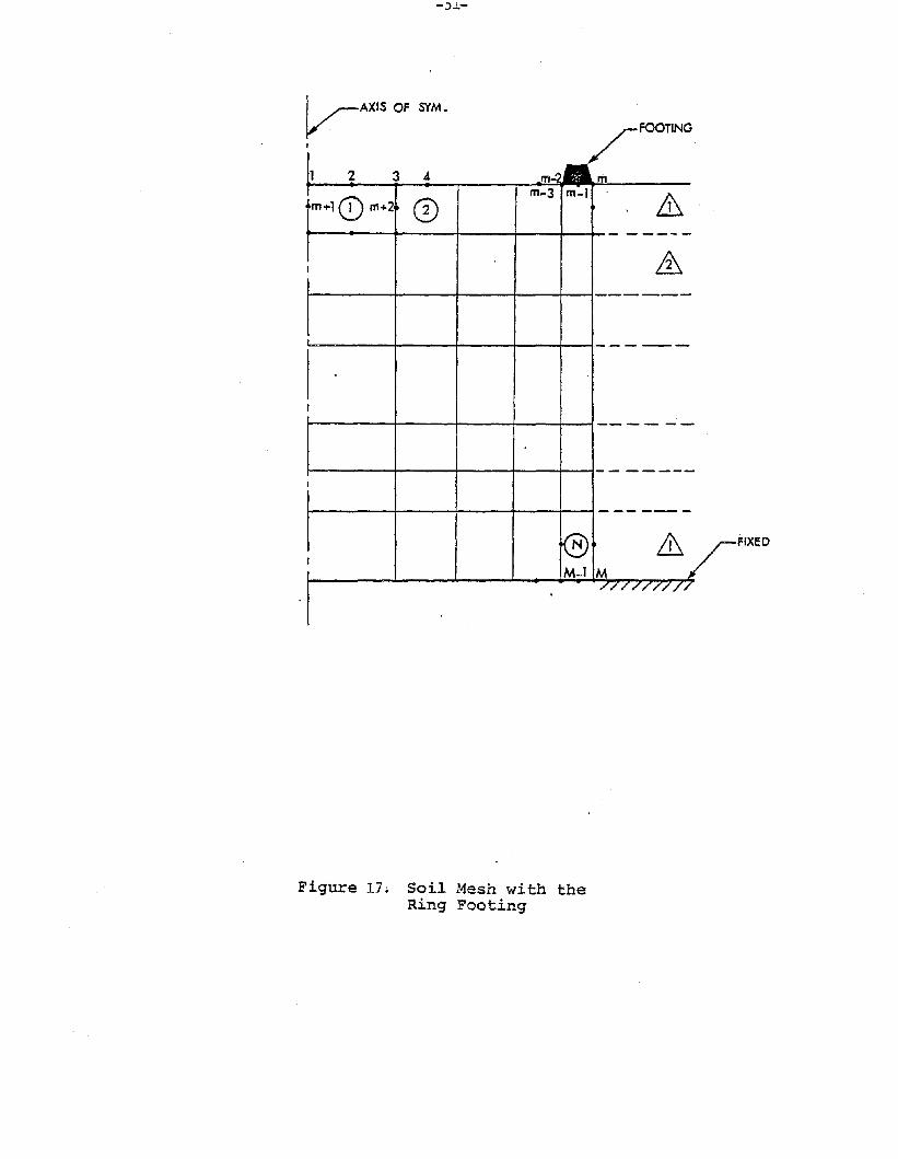
The following cards are the nodal point cards for the soil elements

and they consist of NE cards, where NE equals twice the total number of

elements in the FE zone (see Figure 17). The total number of elements

must be 4 NL where NL is the total number of layers (if NL=l, for the

elastic half space case, the total number of elements shall be 24 elements).

For each element there shall be two cards, the first containing the

radial coordinates of the eight nodes and the second containing the

vertical coordinates of the nodes (see Figure 18).

The format of either card shall be as follows (starting with element

number one and finishing with element number NE):

Columns

1 - 10

11 - 20

21 - 30

Format

FlO.O

FlO.O

FlO.O

Entry

Radial (vertical) coordinate of 1st node

DO for 2nd node

DO for 3rd node

71 - 80 FIO.O DO '" for 8th node

d) The last group of cards in this section is the 'Fourier Harmonic

Numbers Cards', one card for each harmoinc. The total number of these

data cards group is equal to the total number of harmonics specified

in the problem control card. However if columns 11 - 15 in the 'Soil

Control Card' are not blank, only the limit number of harmonics must

be supplied.

The format of the 'Fourier Harmonic Numbers Cards' are as follows:

Columns

1 - 5

Format

15 Harmonic number

Note: For soil analysis, only harmonics zero and 1 are available.

-.:>.L-

FIXEO

/FOOTING.

V-AX1S OF S'fM.

1 2 3 .:1 m-.m

1m+l Q) m+2m-3 m-l .

&CD- -----

I .&----

. -----

I

---- --

-- -----I

------

~ &I

M-I M/////////

Figure 17; Soil Mesh with theRing Footing

,..---------------JlI~ r2

z

Figure 18. Isoparametric QuadraticSolid Element

J. Loading Information Cards:

For each harmonic, there shall be one title card, the 'load -

title card', followed by a control card, the 'loading control card'.

These cards are further followed by one or all of the following

sets of additional cards, excepting in the case of analysis types

1 and 3.

a) Distri.buted Loading Cards - For each region, extending over one

or more elements, one card is required with the distributed loading Fouriet

coefficients being either constant or linearly varying between the first

and last nodal points of that region.

b) Concentrated Loading Cards - One card is required for each nodal

point.

c) Thermal Loading Cards - For each temperature region) extending

over one or more elements, one card is required with the thermal Fourier

coefficients being either constant or linearly varying between the first

and las~ nodal points of that region.

d) Displacement Cards - For each node With specified displacements,

one card is requi~ed. The maximum permissible number of specified dis-

placement components happens to be ten.

The format for the Load Title Card shall be as follows:

Columns

2 - 80

Format

A Any alphanumeric informationidentifying the load

The information to be supplied on th~ Loading Control Card ~re -the

harmonic numbers (0,1,2,3, etc.), the numbers of distributed loading cards,

concentrated nodal loading cards, thermal loading cards and displacement

cards to follow, printout option code (0, or 1, or 2, or 3), gravity

loading option, reference temperature (i.e. stress free temperature, and

the angle which· the line of symmetry for loadinlt makes with the e • 00 line).

The gravity loading option (valid for static analysis only) is

applicable to harmonics a and 1 only. If it is desired to include

the effect of gravity loading (or a fraction thereof), it is necessary

to set the gravity loading option equal to the weight density of the shell

material (or an appropriate fraction thereof). This option .. applies to the

zero harmonic when the gravity loading is in Z-direction and to

harmonic number 1 when it is in the R-direction. If static an~ysis

due to gravity loading is not desired, the corresponding columns in

the loading control card should be left blank. No distributed loading

cards are required for ~avity loading.

Printout opt1l1n"codes'control the output in the following manner.

Printout Option Code

a

1

2

3

Description of Printout

- No result will 'be printed for thecurrent harmonic loading case

- Printout will be provided for thecurrent harmonic loading only

- Printout will be provided for thesubtotal results of all harmonicloadings up to and including thecurrent harmonic loading

- Printout will be provided for thecurrent harmonic loading and alsothe subtotal results of all harmonicloadings up to and including thecurrent harmonic loading

.,

Regardless of the printout option codes specified for different

harmonic loading cases, a printout of the total results is automatically

provided after the final harmonic loading case is completed. The user is

cautioned that codes 1 and 2 may produce very volumnious output if several

harmonics are present.

The format of Loading Centrol Card for each harmon±~will be as fol-

lows:

Number of distributed loading cardsto follow

Harmonic number

Number of concentrated loading cardsto follow

Number of displacement cards to follow(Maximum .. 10)

Number of thermal loading cards tofollow

Print-out option co~e

Reference temperature

Gravity loading option(Blank or weight density)

Columns Format

1 - 5 IS

6 - 10 IS

11 - 15 IS

16 - 20 I5

Zl - 25 IS

26 - 30 IS

31 - 40 FlO

41 - SO FlO

51 - 60 FlO Blank, if loading is symmetricalabout e .. 0 0

90.0» if loading is symmetricalabout e .. 90 0

With respect to the data in· columns 51-60, it may further be stated

that if, for instance, for a particular harmonic the loading in the

u-direction and w-direction consists of a cosine term and that in

v-direction a sine 1:ertn» these columns should be left blank. On the

other hand, if the case is reversed, i.e., the sine term is

associated with the u-direction and w-direction and the cosine term

with v-direction, the value in these columns should be 90.0. In the

-following cards the paren1:he1:1cal values of e refer 1:0 the 1at1:er case.

The format of Distr1.buted Loading Cards for each harmonic will be as

follows:

Columns

1 - 5

6 - 10

u - 20

21 - 30

31 - 40

41 - 50

51 - 60

61 - 70

Format

IS

FlO

FlO

FlO

FlO

FlO

FlO

Entry

Nodal point where loading begins

Nodal point where loading ends

Magnitude of distributed loadingFourier coefficient in u-di.rec:tionat the beginning of nodal point ate .. 0° (or e .. 90°)

Magnitude of distributed loadingFourier coefficient in u-directionat the ~ nodal point at e .. 0°(or e .. 90°)

Magnitude of distributed loadingFourier coefficient in v-directionat the beginning nodal point ate .. 90° (or e .. 0°)

Magnitude of distributed loadingFourier coefficient in v-directionat the end nodal point at e .. 90°.(or e ..()'O)

Magnitude of distributed loadingFourier coefficient in w-directionat the beginning nodal point at&.. 0° (or e .. 90°)

Magnitude of distributed loadingFourier coefficient in w-directionat the end nodal point at e .. 0°(or e .. 90°)

The format of-Concentrated Nodal Circle Loading Cards for each har-

monic will be as follows:

Columns

1 - 5

6 - 15

16 - 25

26 - 35

Format

IS

FlO

FlO

FlO

Nodal point number

Fourier coefficient of line loadin u-di.rection at e .. 0° (or e .. 90°)

Fourier coefficient of line load inv-direction at e .. 90° (or e .. 0°)

Fourier coefficient of line load inw-direction at e .. 0° (or e .. 90°)

Columns Format Entry

36 - 45 FlO Fourier coefficient of line load inB~ direction at e :z 0° (or e .. 90°)

46 - 55 FlO Fourier coefficient of line load inBe direction at 0 ::I 90° (or e .. 0°)

The format of Thermal Loading Cards for each harmonic shall be asfollows:

Columns ~ Format

1 - 5 Nodal point where the thermal loadbegins

6 - 10 I5 Nodal point where the thermal loadends

11 - 20 FlO Magnitude of the~ surface tem­perature Fourier coefficient at thebeginning node point

21 - 30 FlO Magnitude of the inner surface tem­perature Fourier ~icient at thebeginning node point

31 - 40 FlO Magnitude of the outer surface tem­perature Fourier co;t£icient atthe ~ node point

41 - 50 FlO Magnitude of the inner surface tem­perature Fourier coefficient atthe ~ node point

FlO51 - 60 Coefficient of thermal expansionfor t:he region ._

The format of·Displacement Cards for each harmonic will be as follows:

Columns Fomat Entry

1 - 5 IS Node number

6 - 15 flO Fourier coefficients for u-displacementat e .. 0° (or e .. 90°)

16 - 25 flO Fourier coefficient for v-displacementat e -. 90° (or e - 0°)

26 - 35 FlO Fourier coefficient for w-displacementat e ::I 0° (or e .. 90°)

36 - 45 flO Fourier coefficient for Brrotationat e ::I 0° (or e .. 90°)

46 - 55 FlO Fourier coefficient for Be-rotationat e ::I 90° (or e :or 0°)

-JO-

K. Control Cards for Dynamic Analysis by Direct Integration:

Omit this section if the analysis type is not equal to 4. In

most cases, it is very helpful to run a free vibration analysis

(Type 1) before carrying out a Type 4 analysis. The following cards

are needed under this group.

a) The first card, c;.a1led the 'direct integration scheme

card', states the integration scheme to be used and the values of control

parameters for the scheme. The details of three alternative schemes are

given in Appendix 1).

The code numbers for integration schemes,

Single step higher derivation scheme 1

Modified single step higher derivationschem~ 2

Four-step scheme .3

The format of Direct Integration Scheme Card shall be as follows:

Columns Format Entry

1 - 5 IS Code number for integration scheme(1, or 2, or 3) Default scheme: 2

6 - 13 FS *Value parameter P1

14 - 21 FS Value parameter P2

22 - 29 F8 Value parameter P3

30 - 37 F8 Value parameter P4

3S - 45 FS Value parameter P5

46 - 53 FS Value parameter P6

54 - 61 FS Value parameter P7

62 - 69 F8 Value parameter P8

* For values of parameters P1 to PS see _;b.ppendix Do. _ !n the case ofthe default scheme (Code number = 2)>> P1 is taken as 1.4.

-::>~-

b) The next card is called t.he 'data card for dynamic

analysis'. It contains the coefficients (CG and Cl) of the proportional

da1ll9ing mat't'u - (CO~ls scalar multip~ier for time functions total .

numbe't' of records in the input time function, number of different time

step lengths to be used, number of time steps between the printing and

the plotting of stress resultants, displacements, etc., number of har-

monics for which the time histories are to be plotted, the initial and

final step numbers for plotting histories, the plotting device to be

used (line printer or the Calcomp plotter) or the punched output cards,

printer plot spacing, and code number which signifies whether or not the

analysis is being > carried out for base acceleration.

The format of Data Card for Dynamic Analysis shall be as follows:

Columns Format

1 - 10 FlO

11 - 20 FlO

21 - 30 flO

31 - 35 IS

36 - 40 I5

41 - 45 IS

Coefficient 'CO t of proportionaldamping matrix

Coefficient ' ('''1' of proportional.damping matrix

Scalar multiplier for eheinput:time function

Total number of record prints inthe input time function

Number of different time step lengthsto be used (Maximum· 4)

Number of time steps between theprinting of maximum displacements,stress resultants, etc.

46 - 50 . IS Number. of time steps between ~he

printing and plotting of displacements,stress resultants, stress components,etc.

Columns

51 - 55

56 - 60

61 - 65

66 - 70

71 - 75

76 - 80

Format

15

15

15

15

IS

IS

-vv-

Number of harmonics for which the historiesare to be plotted

The initial time step for plotting thehistories

The final time step for plotting thehistories

Code number of plotter ( = 1, printer plot;= 2, Ca1comp plot). If blank punched outputwill be generated.

Printer plot spacing (Default = 1)

1, loading is due to base acceleration;otherwise leave blank

The above card may be repeated for each harmonic provided that the

column 35 in the problem control card is not left blank.

Note: The punched cards option can be very useful as the plotting sub-

routines are installation dependent (see the overlay structure of

Figure 4) and by choosing such option one may use the punched time

history with the appropriate local plotting routine available. A ~lotting

Program suitable for a 760/563 Calcomp Plotter system is given in

Appendix F (Program 'TRPLOT').

c) The next card, called the 'initial condition control card',

specifies whether the nodal displacements, or velocities or accelerations

are non-zero at the starting time.

The format of Initial Condition Control Card shall be as follows:

Columns Format ~

1 - 5 15 1, if the in~tial nodal displacementsare non-zero; otherwise leave blank

6 - 10 IS 1, if the initial nodal velocitiesare non-zero; otherwise leave blank

11 - 15 IS 1, if the initial nodal accelerationsare non-zero; otherwise leave blank

-O.l.-

In the above card only one of the three responses may be taken

as non-zero. In the case of earthquake loading it is preferable to use

a blank card.

d) The following card, called the 'time step control card', gives

the time step length and the record point number of the input time function

up to which it is to be used. A maximum number of five time steps can be

specified, provided that all time steps are integral multiples of the

smallest time step specified. In order to reduce the effect of artificial

damping introduced by the integration scheme it is desirable that the

maximum time step length used be not more than, say, one-tenth the

smallest natural period.

The format of Time Step Control Card shall be as follows:

Columns Format Entry

1 - 10 FlO First time step

11 - 15 15 The last record point number, for thisstep, in the input function

16 - 25 FlO Second time step

26 - 30 15 The last record point number, for thisstep, in the input function

etc. etc. etc.

Note: In the case of a fixed foundation, one should be especially

careful in choosing the time steps for the numerical integration.

Relatively large time steps may cause numerical instability and the

solution may diverge instead of converging (see Example number 8).

e) The next card is the 'title card·for input time functiou'. This-

card is required only if the column 30 of the Output Control Card is

net left blank.

-0"::-

The format of Title Card for Input Time Function shall be as follows:

Columns

2 - 72

Format

A Alphan~ric information about the loadfunction

f) The next card (or cards), called the 'record points card',

provides the record points of the time history input function, which may<#

be the multiplication factors for any mechanical or thermal loading or

the base acceleration (vertical or horizontal) due to earthquake. In the

case of multiple loading, the multiplication factors should reflect the

net effect of all the components. It is necessary to provide this card

(or cards) for each harmonic only if these factors are different for

different harmonics and column 40 or Problem Control Card is not left

blank.

The format of Record Points Card(s) shall be as follows:

Columns Format Entry

1 - 10 FlO Time

11- 20 FlO Value

21 - 30 FlO Time

31 - 40 ~10 Value

etc. etc. etc.

There can be a maximum of four pairs of data per card.

-oj-

L. Data Cards for Dynamic Analysis by Response Spectrum

~ this section if the analysis type is not equal to 3.

a) The first card is the 'modal damping ratio card' and gives the

damping ratio to be used for each mode.

The format of Modal Damning Ratio Card shall be as follows:

Columns Format Entry

1 - 5 15 Mode number

6 -15 FlO Damping ratio

16 - 20 IS Mode number

21 - 30 FlO Damping ratio

etc. etc. etc.

Each damping ratio card may contain a maximum of five pairs of

data. ''the maximum number of modes that can be considered has

been limited to ten.

b) The next card, to be called as the 'response spectrum data title

card', is needed only if the column 30 of output control card is not left

blank.

The format of Response Spectrum Data Title Card shall be as follows:

Columns Format

A2 - 72 Any alphanumeric information des­cribing the response spectrum data

c) The neX1: card, ca'lied the 'e.o:tltr~l'.ca·rd for ,response- .

spectrum', gives information such as the number of damping ratios for ,which

the data is given, the number of record points for each damping ratio,

whether the data consists of spectral velocity or spectral acceleration,

and the scale factor for the spectral values.

The format of Control Card for Response Spectrtml shall be as follows:

Columns

1 - 5

6 - 10

11 - 15

16 - 25

Format

IS

IS

IS

FlO

Entu

Number of 'damping ratios for wh:Lch re­sponse spec1:rum data is given (Max­imum :I 8)

Number of record points for eachd.a.mPing ratio

1, if spectral velocity is given2, if spectral acceleration is given

Scale factor for spectral values(Default • 1)

d) The next card gives the values of damping ratios corresponding

to which the response spectrum data is given.

The format of Spectral Damping Ratio Cards shall be as follows:

Columns Format Entry

1 - 10 FlO Damping ratio no. 1

11 - 20 FlO Damping ratio no. 2

21 - 30 FlO Damping ratio no. 3

31 - 40 no Damping ratio no. 4

etc. etc. etc.

e) The following cards, called the tspectral value,. cards , ,

give the frequencies (starting from the highest and going towards the

lowest) and the corresponding spectral values correspondi:ng.tG each damping

ratio at a time starting with damping ratio no. 1.

The format of Spectral Value Cards shall be as follows:

-0;.1-

Columns Format Entry

1 - 10 FlO Frequency (Hz)

11- 20 FlO Spectral value

21 - 30 FlO Frequency (Hz)

31 - 40 no Spectral value

etc. etc. etc.

There can be a maximum of four pairs of data per card.

-00-

M. Last Control Card:

This card signals termination of job and is the last data car.d t.o

be provided in a job. Preceeding this card the data cards for any number

of problems can be placed.

The format of Last Control Card shall be as follows:

Columns Format Entry

1 - 6 A JlbBEND

SIlORE-IYP,ROGRAM 'OUTPUT

Typical examples of actual ou~put will be supplied on request,

Printouts for Input Data;

All input data for each problem are printed out in suitable formats

in order that the user can verify them easily. Moreover, as mentioned

earlier, an echo (i..e. card image) of the input data can also be printed

out.

Various checks are performed by the program internally and obvious

errors cause a run to terminate, after printing out the error messages,

before execution of the probl~ takes place.

Printouts for Results:

In the case of Static Analysis, the results of computations printed

out: by the program 0, a:re'comprised:o£ :th,e' £91l0win"g: _

1) For each harmonic number, a table of nodal point displacement

components Cu, v, w. e~ and ee, for sign conveut±on see Figure 2 ) is

printed out together with Z-location of all nodal points.

2) Depending, on the printout option code specified in the Loading

Control Card for a harmonic loading case, tables o~ displacements, stress

resultants (N~, Ne, NiPe, HiP' Me, QiP' and Qa, for sign convention see

Figure 1 ), and stress components (a~, aa, a$6' aI' 02 and aeq) are printed

out: for each e.lement at the nodal points and at the specified number of

intermediate points. The stresses SIGMA(l) (i.e., ( 1) and SIGMA(2) (i.e.,

( 2) are the. principle. stresses"wb:~ ,S!GMA(EQUI) (i..e..) <!eq) is an

equivalent stress, corresponding to von Mises-yield criterion, defined by

-68-

the expression

0'eq

The meridional length of the element and its thickness at the top and

bottom nodes are also given. The non-dimensionalized arc length variable

s is used to define locations along each meridian curve and this variable

ranges from 0 at the top to 1 at the bottom node of an element. In the

case of open-type elements the displacements and forces

M ,Y

F.... , Fy ' F , M ,.... z x

and M (for sign convention see Figure 3) at the end o·f the membersz

are printed out. Moreover, the length(s) of the member(s) is also

printed out.

In the case of Free Vibration Analysis. the results printed out by

., the. program. m~y .1X1clude.• the .. following.:. ..

1) A table giving information on isolated roots is printed out. If

in the first line of this table, the number of roots with

values less than the upper limit for P (i.e. Pu) happens to be

less than the order of stiffness or mass matrix, it signifies

that number of lowest frequencies e~l to the difference has

been missed. In that case, the problem should be rerun after

suitably increasing the value of Pu•

2) The eigenvalues, circular freque~cies (rad/sec), and cyclic fre­

quency (Hz) for all the desired modes in each harmonic are

printed out.

3) Depending upon the printout option used in the Eigenvalue Analysis ..

Card, the normalized eigenvectors corresponding to each mode are

printed out.

-b~-

In the case of Response Spectrum Analysis, the results of computation

printed out by the program may comprise of the following:

1) Results same as those for the .Free Vibration Analysts a:r~printed.out.

2) Tables of maximum displacements, accelerations, and stress resul­

tants for each mode are printed out.

3) Tables of root mean square values of maximum displacements,

accelerations, and stress resultants for each mode are printed

out.

In the case of Time History Analysis by Direct Integration, the re­

sults of computation printed out by the program may include the fol­

lowing:

1) Depending upon the printout option codes specified in the Time

History Output Control Card, tables of absolute maximum displacements,

and/or accelerations (relative or total), and/or stress resultants are

printed out for each harmonic. !he time instants at which such maxima

occur are also printed out in the same table. If, however, the bottom

element of the shell happens to be open-type, the stress resultants

at the base of the shell are printed out as zero, irrespective of

the support conditions of the members'of the open type element.

Again, if the maximum responses at a given number of time step intervals

are desired, similar tables with the time range number stated therein are

printed out.

2) If the relevant option code is specified in the Time History Control

Card (and Loading Control Card), stress resultants, stress components,

and displacements at a specified number of time step intervals1n the form

of tables similar to those described for static analysis are printed out.

The instant of time for which the values are valid are also printed out.

Plots for Time History Response:

Two alternative kinds of plots are possible, namely the printer plot

and the Calcomp plot. The plots can be for the displacement Fourier coeffi­

cient history, and/or the total acceleration Fourier coefficient history,

and/or the stress result:ant Fourier coefficient history. Before actual

plotting is done the components to be plott:ed, their maximum values, and

the instant of time when the maxima occurs are tabulated. The components

are defined by the node and the component: numbers 1, 2, 3, 4, and 5, which,

respectively, stand for the components along u, v, w, S4>' and Se in the

case of displacements and accelerations, and N4>' Ne, M4>' Me, and Q~ in the

case of stress resultants. First the plotting is done for the individual

harmonics and is then followed at the end by resultant plots for all the

specified harmenics corresponding. to the refe.rence position e sa 0°.

When the Calcomp plot option is specified r a table of plotted values,

for each harmonic only are printed out. In this case the program actually

creates a plot tape to finally carry out off-line plotting on a 760/S63

Calcomp plotter system.

Time Log Printout:

At the end of each problem a time-log for the problem is printed out.

The time-log states the CPU time in seconds required to execute different

sections of a problem.

-71-

ACKNOWLEDGEMENTS

This work was partially supported under NSF Grant No. PF~-7900012..-=

However. any opinions. findings. conclusions or reco~endations expressed

herein are those of the authors' and do not necessarily reflect the views

of NSF.

The authors gratefully acknowledge the cooperation of Washington Uni­

versity Computing Facility staff.

-U.-

APPENDIX A

SYSTEM CONTROL CARDS

The image of the system control cards used to run SHORE-IV from

permanent file (WU65(i1E.SH(i1RSS) at WashingtonpniverSity Computing Facility

using an IBM 360/65 computer is shown below. If, in the case of time

history analysis by direct integration, the printer plot option is used,

the last four devices are to be ~eplaced by three scratch tapes (Nos. 26,

27, 28 with data set names NTAP8, NTAP9, NTAPIO, respectively).

IIA EXEC FORTRAN.LIBRARY=·WU6S0E.SHORSS·,PROGRAM=SHORSSIIGO.FT09FOOI -00 U~IT=SYSOA.SPACE=(TRK,(2S.51,RLSEI .OCB=(RECFM~YBS,II LRECL=84,BLKSIlE=844 6UFNO=11IIGO.FTIOFOOl 00 UNIT=SYSOA,SPACE=l72,(5,111,OCB=IRECFM=VBS,LRECL=68,II BLKSIlE=72 BUFNO=31IIGO.FTIIFOOI 00 UNIT=SY~OA,SPACE=(TRK,(l,l)1,OCB=(RECFM=VBS,LRECL=112,II BLKSllE=188,3UFNO=11IIGO.FT12FOOl DO UNIT=SYSOA,SPACE=(TRK,(lS,SII,OCB=(RECFM-VBS,II LRECL=1148,BLKSIlE=11S2,BUFNO=11IIGO.FT13FOOl 00 UNIT=SYSOA,SPACE=(TRK,118,111 ,OC8=(RECFM=VBS,II LRECL=3700,BLKSIZE=3704,BUFNO=11IIGO.FT14FOOl 00 UNIT=SYSOA,SPACE=ITRK,(6,111 ,OCB=(RECFM-YBS,I I LRECL= S204, BLKS I ZE=S208, 8UFNO=l)IIGO.FT15FOOl DO UNIT-SYSDA,SPACE=(TRK,(lO,71 ,RLSEI,OCB=(RECFM-Y8S,II LRECL=S24,BLKSIZE=S28,8UFNO=11IIGO.FT16FOOl DO U~IT=SYSOA,SPACE=(TRK,15,11,RLSEI,DCB=(RECFM=V8S,II LRECL=1604,8LKSIZE=1608,8UFNO=11IIGO.FT17FOOl 00 UNIT=SYSOA,SPACE=(TRK.(S,21),OC8=(RECFM-YBS.II LRECL=1156.BLKSIlE=1160,BUFNO=11I/GO.FTl8FOOl DO U~JI T=SYSOA,SPACE=( TRK, (10 ,SI ,RLSEI ,OCB=·( RECFM-YBS,II LRECL=1148,8LKSIZE=1152,BUFNO=11IIGO.FT19FOOl 00 UNIT=SYSOA,SPACE=(TRK,(S,SI,RLSEI ,OCB=(RECFM=YBS,II LRECL=164,BLKSIZE=168,BUFNO=11IIGO.FT20FOOI 00 UNIT=SYSOA,SPACE=(TRK,IS,SI,RLSEI,DCB=(RECFM=VBS,II LRECL=324,BLKSIZE~328,BUFNO=11IIGO.FT21FOOl DO UNIT=SYSOA,SPACE=(TRK,15,51,RLSEJ ,OC8=(RECFM=VBS,II LRECL=324,BLKSIZE=328,BUFNO=11IIGO.FT22FOOl 00 UNIT=SYSOA,SPACE=(TRK,(l,ll,RLSEI ,OCB=(RECFM=YBS,II LRECL=84,8LKSIZE=340.BUFNO=11IIGO.FT23FOOl 00 UNIT=SYSOA.SPACE=(TRK,(S,SI,RLSEl,OC3=(RECFM=VBS,II LRECL=324,8LKSIZE=328.8UFNO=11IIGO.FT24FOOl 00 UNIT=SYSOA,SPACE=(TRK,(5.SI,RLSEl .OCB=(RECFM=VBS,II LRECl~324.8LKSllE=32a,BUfNO=11IIGO.FT2SFOOl 00 UNIT=SYSOA,SPACE=(TRK,(5,51,RLSEJ ,OC9=(RECFM=VBS,II LRECL=324,BLKSIZE=328,8UFNO=11IIGO.FT26FOOl 00 UNIT=SYSDA,SP.\CE"( TRK,(S,SI ,RLSE) ,DC8=(RECFM=VBS,II LRECL=804,BLKSIZE=808,BUFNO=11IIGO.FT27FOOl 00 ONIT=SYSOA,SPACE=(TRK,IS,SI,RLSE1,OC3=(RECFM=ves,II LRECL=804.BLKSIZE=808,BUFNO=llIIGO.FT28FOOl 00 UNIT=SYSOA,SPACE=(TRK.(S,SI,RLSEI ,OC8=(RECFM=YBS,II LRECl=804,8LKSIZE=80a,BuFNO=11IIGO.PlOTTAPE DO OSNAME=PLOTTAPE,UNIT,.TAPE98.VOL=SER=420S61,OC8=OEN=2,II OISP=(NE~,KEEPI,LAeEL=(l,SLI

IIGO.SYSlN 00 *

-7"3-

APPENDIX B

ELEMENTS OF CONSTITUTIVE MATRIX

The elements of constitutive matrix [C] for isotropic and single-layer

orthotropic shells are given below.

Isotropic Single-layer.Orthotropic

c­·33

.(:55

C77

Caa

"

A.h1.

2(1-11)A.h.~

A.h3/12.1. .'.

A.h3/121.

A(l-lJ)A.h/2.J.

A h,o'

P,e Aoh

P.::.t! A hlJa, 0

4 G,eh

lJ,a Aoh3~12.

~lJa, Aoh3/12.

Ai = E/{1-112); h =total shell thickness

A = shear factor (to suppress transverse shearing strains, i.e.IG.r~hhoffhy"pothesis, set ;\.=100)

A =:Elb,;,- 11 0}1.)o ." . 'a, cpa .

Etfl =Young's modulus in 4l-direction

lJtfla

, l1e, =Poisson!s ratins for ~ or '9 directions with respect toe or , directions

GipO' Gipn' Gan =the shear moduli for ~-&, ~-n, and e-n planes

-1'+-

The elements of constitutive matrix (el for multi~layer orthotropic

and framed shells are given below.

Multi-layer Orthotropic.. . . Framed

Cl2

. C,,33

C,45

CS5

C:66

0.77

·C aa

o

o

(A ) ,etc. =the value or A , etc for layer 'k'ok' . 0

=thickness of layer 'k'

=the distance from the centroid of layer k to middle" sUrfa:ce', assuming symmetrical layers (see Fig. 5)

A~, Ae

~41' Ked d41' eE, G

= the area of members of frame in ~,e directions

= St. Venant torsional constants in ~,a directions

=the spacing of meridional and circumferential members

= Young's and Shear moduli

-75-

APPENDIX C

INTERMEDIATE PRINTOUT OPTION CODES

Code No.

86

87

88

89

90

91

92

93 .

Ref. Subroutines

GLMX

FIN'AFMINAESOTEMOT

GLMX

CALQF

ARC

LASH

SSTMST

Description of Intermediate Printout

Upper diagonal part of structure stiff­ness and mass matrices in banded formas arrays GS (1 to N) and GM (1 to N).Where, N =0 6x (no. of nodes) for j = aand lax (No. of nodes) for j > O. Theelements of these matrices need to bemultiplied by 27T for j = 0, and by 7T forj > O.

Upper diagonal part of improved elementstiffness and mass matrices as arraysA and AM or BM. The elements of allthese matrices need to be multiplied by27T for j = 0, and by 7T for j > O. More­over, the elements of A need to be mul­tiplied by a fac~or 106 .

Structure loading vector as RF (1 to M)array. Where M =5 x (No. of nodes) forj > 0, and 3 x (No. of nodes) for j =0 O.The elements of all these vectors shouldbe multiplied by 2rr for j = 0, and by rrfor j > O.

Element nodal loading vector as QF (1 to6) and QFC (1 to 10) arrays correspondingto harmonic numbers j = 0, and j > 0,respectively.

Local of nodes and three intermediatepoints on the meridian of each elementwith respect to the global coordinatesystem.

Temperature loading data for an element.Printout is in the form of an arrayIX (1 to 30)*.

Section properties of multi-layer ortho­tropic material as AS (1 to 7)** array.

Coefficients of Direct Integration Scheme.

* TX(l) to TX(S) and TX(16) to TX(19)

TX(6), TX(12) , TX(14)

= Temperature data

= Elastic and thermal properties

TX(7) to TX(ll) and" TX(lS) = Geometric data

TX(20) to TX(30) = Thermal loading data. For furtherdetails see subroutine TEMP. "

** AS(l) = Overall thickness

AS(2) =" Equivalent area per unit length ofmiddle surface in terms of outerlayer (ep- direction)

AS(3) = - do (a-direction)

AS(4) = - do (4)a-direction, for shearstress calculation due to N</>a)

AS(5) = EquiValent moment of inertia perunit length of middle surface interms of' outer layer (ep-direction)

AS(6) = - do (a-direction)

AS(7) = - do (4)6-direction, for shearstress calculation due to Mepe)

-77-

APPENDIX D

-

1.. Single Step Higher Derivative Schemes.[4 J:

After the stiffness matrix [K] and mass matrix [M] has been formed,

it is necessary to evaulate the following constants.

1-

1(-- 1)2P1

A •9

~o·

1

1

-78-

1~1:a (- -1)2PI

~2'"

P2PI ~t

P2 )Al3

... (- - IPI

where

PI' P2 , P3 = the parameters of integration scheme

~t = the time step

:a the coefficients of Rayleigh damping matrix

Next, it is necessary to form the modified stiffness matr~ It is

fo1low~d by forward elimination•

..[K] ... [Kl + ~ [M]

Then, the modified load vector is formed as below... 1~3{F(t:+~t)} = {F(t+~t)} + -p- {F(t:)}

3..

+ [M] (A3{~(t)} + A4{~(t)} + A5{~(t)})

-79:-

-Finally, the displacements {~(t+A't)} are calculated by back substitution.

Thus,

and the true displacement vector at time't+At' will then be

the corresponding velocity and acceleration vectors are then calculated from

- ~{A(t+At)} 2 ~{A(t+At)} - ~{A(t)} - ~O{!(t)} - ~{A(t)}

In the case of Newmark's ~method, P3 '" 1. For Wilson's 6-method,

Pl 2 1/6 and P2 '" 1/2. For an unconditionally stable scheme, in the first

case. one should take Pl '" 1/4 and Pz '" 1/2. and in the later case P3 = 1.4.

-ou-

2. Multistep (3,-step) Schemes[4].:

Here the constants to be evaluated are

( l+ PlCi)at

P2(C~-c-l~ )

at

P (c·-c A...)3 '0 r-r.

At

A •6

where PI' P2' etc. are the parameters of integration scheme.

Here the· modified s~iffness matrix and load vector will be

-{F(t+at)} ,. {F(t+at)} + [M] (A3{a(t)} +

-81-

_.As in scheme l~ after solving the following for {~(t+6t)}

the displacement vector is calculated from

+ Ag{6(t-2At)}) / AZ

In the case of first time step~ i.e. at t"'At~ it is necessary to

modify some of the aforementioned constants as below.

c ...2

~* .. (~A2 - C2) I (A2

- Cl

)

...

A3* .. (AlAZ - CZ) I (A

Z- C

1)

...A

4* a (A3 - P

2C

3)

For this step~ Ar~ A3, A4, and AS are to be replaced ~Y Ar*, ~*,

A4*, and AS*' Moreover, it is necessary to evaluate the following

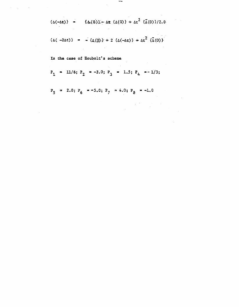
{A(-At)} a

In the case of Houbo1t's scheme

p "" 11/·6· p. - -3· o· P "" 1 5· P .. -i/-3·1 '2 ·'3 e'4 '

-83-

APPENDIX E

LISTING OF 'FORHAM' (Program for calculating Fourier Coefficients)

c **•••••••••••**.**.*** ***•••***.MAINOOOlC MAI~0002

C THIS IS THE MAIN :a~TROl. PROGRAM FOR CALCULArtNG FOURIER COEFS FORMAIN0003C A~ AAI8TRARY LOAD FUNCTION DISTRIBUTED AROUND THE CIRCUMFERENCe MAI~OOO~

C FOR TWO SITUATIONS 14AIN0005C . 11 WHEN THE ORDINATES ARE GIVEN AT EQUAL INTERVALS MAIN0006C AND THE NUMBER OF ORDINATES A~e EQUAL TO THE MAI~0007

C NUMBER OF FOURIER coefFICIENTS (Ifl*OI MAIN0008C ZJ WHEN EITHER THE NUMBER OF ORDINATES ARE DIFFEREHTMAIN0009C FROM THE DeSIRED NUM8ER OF FOURIER COEFFICIENTS MAINOOI0C OR THE INTERVAl.S BETweeN THe ORDINATes ARE NOT iliA ["10011 ..C EQUAl OR BOTH (IF\.>()) MAIN0012C MAIH0013C PROGRAMMEO a y; MAlNOOl4-C PRODYOT KUMAR BASU MAI~0015

C WASHINGTON UNtVERSITV MAl~0016

C AUGUST, 197& . MAINOOl1C MAIN0018C •••*•••••••••••••••••••••••••••••••••, •••••••••••••••••••*••••*•••MA{~OOl9

IMPLICIT REAL.8 (A-H,P-I) MAIN0020OIMENSION VALI50.,A~G(501,X(50J,Y(50t,H(~50),A(25l.B(25),P(50), MAIN0021

x HEO(ZOI,CCZOO,25l ,T(ZQOl.OtZ5,2001 HAI~0022

C HAIN0023C ttl = "fUMBEIt Of DATA 50S rQR WHICH FOURIER coeFFICIENTS ARe MAIN0024C ReQUIREO MU~0025

C ~OIM s NUMBER OF GIVEN ORDINATES (AT Eg~AL INTERVALS OR OTHERWISElMAIN002bC , P~OV10EO THE LAST QRDINATE FOR NS=O CORRESPONOS TO THErA-360 MAINAOZ6C DEGReES, AND THH FOR NS>O TO THEU=lSODEGREeS. MAIN8026C NO = 2 TIMES tHe ~AXIMUH n~oeR OF H4RMONICS TO BE MAINOO?1C rCTTeo p~us 1 (l.E. THE NUM8ER Of COSINE TeRMS MAIN0028C AND SINE TERMS TO ae CONSIDERED + 11 MAI~OOZq

C IF IFL sO: ~a < ~DI~ MAlN0030C IFL a 0, ~O INTERPOl.ATION USING CUBIC SPLINES MA[N0031C ) 0, INTERPOLATION NECESSARY, IF THE ORDINATES ARE NOT AT MAIN0032C EQUAL INTERVAL AND 'NOIM-I' is HOT 000 MAIN0033C NOO a 0, ~O PUNCHED OUTPUT OF TIME HISTORY OATA MAIN0034C 1,PUNt~ED OUTPUT OF TIME HISTORY DATA REOUIRED MAI~003S

C IF NOO s 0, PUT NHC • O. AND NHS a 0 MAIN0036C IF NOO • 1, ~HC * NUMBER OF HARMONICS(COS, TO BE PUNCHED 8EGINNING~AIN0037

C wITH THE ZEROETH; MAXIMUM VALUe. (NO-11/2 + 1 MAI~0038

C NHS • Nu~eER OF HARHONIC~(S[N' TO aE PU~CHEC 8EGtNNtNGMAtNQQ39C WlTHTIiE FIRST; 14AXI14lJ,'l • INO-l l/2 MAIN0040C lDF • 0, OATA IS INPUT TIME STEPWISE MAIN0041C IOF 2 1, OlTA IS INPUT POINlwISE MAIN0042C TIl" INITIAl. TIME INEEDED IF NDO=U MUN0043C r5 • TIME STEP (NEEOeO IF NOO=L) MAIN0044

TII=O.O MAIN0045T5=0.0 MAtN0046AMIN s 1.000 MAI~0047

-0'1--

WIUTE( 6,50150 FORMATCIH1//17H*****ERROR IN iNPUT OATA••••NUM6ER OF FOURIER

~ICIENTS SPECIFIED IS WRONG)

GO TO ZOO60 CONTINUE

NN =< NO/lNM a NO - N~1*2

IF(NM.EQ.11 GO TO 4

P'E ~ 4~ooo*aATANIAMtNI

READe 5,11 HEO ,NI ,NOO" NO, I FL ,tJDO, I~HC ,NHS, IOF1 FORMATI20A4/8151

NHS • NHS + 1IFINOD.EQ.OI GO TO 23REAOCS,21) TII,TS

21 FORMAT(ZF12.61TI a TIl00 ZZ Ial,NITIll :a TI

2Z TI :a TI + TS23 CONTINUe

W~ITeI6,51' NI,NOIM,NO,IFL,NDO,NHC,NHS,TII,TS51 FORMATI7IS,2F12.61

IF(lfl.GT.OI GO TO 60NK = NOlM - 1

iF(NO.LE.NK) GO TO 60

IN nlPUr DA TA****NUM8ER OF FOUR 1ER

cC

C

CW'l I TEl 6,401

40 FORMATlIH11/69H••••*ERRORXICJENTS IS NOT 0001

GO TO 2004 CONTINUE

WRITE(6,ZI HEU2 FORMATIIHL/20h4111

MO • NOiFlIFl.NE.O.ANO.NO.LT.ZSIMOll a 140 - 1NOL 1 .. NO - 1M a NOLl/2)(lll a O.OVlll·0.0PI = Z.O*PVE/NOPlea Z.O.PVE/MOaD 3 101 L, NUL L

3 X(I+ll :a XI I I + PI00 24 I a 1,MOLl

2ft. '11+1) a YIU + PIE

MO=25 •

MAIN0048MAI~0049

MAIN0050MAINOOSl"'~IN005ZMAIN0053"AINOOS4"AIN0055MAI~OOS6

MAIN0057MAINOOS8··MAIN0059MAI~0060

MUN0061MAIN0062MAI~0063

MAIN0064MAlN0065MAIN0066MAI~0067

CO!ffMAIN0068MAIN0069HAIN0070MAIN0071MAINOOT2MAINOOnMAIN0014HAIN0075MAINO()16HA tNOO 71

COEfFMAIN0018MAIN0079MAINOOSOMAIN0081HAtH0082MAIN0083MUNAOS3MAIN80S3MAlNC083HAIN0084MAI~0085

MAIN0086MAIN0087MUNOOSSMAINA08SMAI~0089

MAIN0090MAI~0091

MA.IN0092

REAOCS,SI IARGCII,I::l,NOIMI MAIN00935 FORMATISFIO.61 MAIN0094

C MAIN0095C MAI~OOq6

C MAI~OOq7

C MAIN0098IF( rOF.EQ.OI GO TO 4S MAlN009900 49 K - 1,NOIM MArNOIOOREADC5,431 (e(L,KI ,L::l ,NO MAINOIOI

43 FORMATlSF10.41 MAINOIOZ49 CONTI~UE MAINOI034500 100 NIP - 1,NI MUN0104-

IFC IOF.EQ.lI GO TO 46 "UNOI05READ(S,61 lVALll),I::l,NOIM) MAINOI06

6 FQRMATI8FIO.4) MAIN0107GO TO 48 "AINOIoa

46 DO 47 I::l.NDIM MAINOl0947 VALlI) a ClNIP,I) MAINOIlO48 w~ITEC6,71 ~IP MAINOlll

7 FORMATlI15X,20HI~PUT DATA SET NO.:: ,ISI15X,16HTHETA IN DEGREES,5X,MAINOl12X13HPReSSU~E HEADIII MAINOll3

00 8 l-l,NOIM MAINOl14ARGO:: ARGIII MAINOllSARGCI) ~ ARGD*PVE/180.0 MAINOl16

8 wRITEC6,91 UGD,VALlI) MAIN01179 FJRMATC10X,F10.6,6X,E12.S/I HAINOl18

IF(lFL.EQ.OI GO TO 18 MAINOl19WRITEC6,lOI NIP HAIN0120

10 FORMAT (lHl,5X,66H INTERPOLATED VALUES AS PER CU6lC SPLINE SCHEME MAIN0121X FOR DATA SeT NO.::,ISI15X,lbHTHETA IN OEGREES,5X,26HINTERPOLATEO PHAIN0122XRESSURE HEADIII MAINOL23

C HAIN0124CALL CUBS~LlVAL,ARG,NDIM,MO,y,H,IERI MAI~0125

C MAIN012618 IF({FL.EQ.OI NN :: NDIM - 1 MAIN0127

IFllfL.NE.OI NN :: lola MAlN012axo ~ 0.0 MAIN012900 11 I :: 1,NN "AIN0130IF(IFL.EQ.O) GO TO 25 MAIN0131P(II :: YlII MAlN0132XO :: (I-11*360.0/MO MAIN0133WRITE(6tl21 XO,Y([I MAIN0134GO TO 11 . MAIN0135

25 PCII a VALlI) MAIN013611 CONTINUE MAIN013712 FaRMAT(10X,F10.6,6X~FIO.6/1 MAINOI38

WRITE(6,131 NIP MAIN013913 FORMATCIH1,5X,49H VALUES OF FOURIER COEFFICIENTS FOR DATA SET NO.::MAIN0140

~,I5115~,16H HAR~ONIC NUM8ER,~X,25H COEFFICIeNTS FOR COSIJXI,5X,2SHMAIN0141

x COEFFIC1ENTS FOR SINIJXI/IJ141=14+1CALL FQURIEIPtNN,Ml,A,StIER.PVE)00 15 J-l,Ml1.1. = J - 1WRlTe(6tH) I.l.tA(J),8(JI

14FQRMATII0XtI5t20X,F10.6.20Xt FIO.6115 CONTINUE

IFINIP.EQ.NII GO TO 9900 20 K=L,NOIM

20 A~GIK) = ARGI~I.L80.0/PV=

YllI .. 0.0DQ 30 1=1,140

30 VII+11 = y(tl + Z.PVE/MQ99 CONTINue

IF(NDO.EQ.OI GO TO 9800 3L K:altNHC

31 OINIP,KI = A(~I

IFINS.GT.O) GO TO 98IF(NIP.EQ.1I GO TO 9800 32 K=2,NHSKK = NHC + K - 1

32 DINIP,KKI a S(KI98 CONTINUe

100 CONfI~Ue

IF(NOD.eC.OI GO TO 200NHS = NHS - 1IF(NS.GT.OI NHS=ONH .. tiHC + NHS00 150 K=I,NHWRITE( 7, ltOI K

110 FORMAT(lH tI31IFITII.LT.O.000001I GO TO 140WRITEI7t lZ01 T(ll,Oll,KI,TI2I,OI2,KI,fI31,0(3,KI

lZ0 FORMAT(20X,6FI0.51WRITE(7,1301 ITIJI,OIJ,KI,J=4,NII

130 FORMAT(4(FI0.5,FI0.51)GO TO 150

140 CONTI~UE

WRITE17,1301 ITIJ),OIJ,KI,J=l,NII150 CONT I~Ue

WR IfEl 6, 1601160 FORMATlIH1/40H ••••MEAN VALUES OF FOURIER COeFFICIENTS/II0X,

X34HFOURIER COEFF. NO. MEAN VAlUe/II00 180 Ka l,NItTIKI = 0.000 115 J a l,lIIlTIK) ,. TIKI + OIJ,KIIFIJ.LT.NII GO TO 175

MU!II0142MAlN0143MAIN0144MAIN0145MAlNOl"6MAiN01"7MAfN0148MAIN0149MAIN01SOMAlNOl51MAIN0152MAINA152MAIN0153MAlN0154MAINOl5!)MUN0156MAIN0157MAI~OI58

MUN0159MAIN0160MAIN0161MUN0162MAIN0163MAIN0164I4UN016SMUNOH6MUN0167I4AIN0168MUN0169

. MAIN0110MUNOl7lHAINOl72MAINOl73MAIN0174MAIN0175MAlN0176MAIN0177MAlNOl7aMAIN0179MUNOlaOMAINOlSl",UNOISlHAIN0183MAINOIS4MAINOl8SMUNOla6MAlNOla7MAINOlSSMUNOIB9

AFC a TC KIINlWRITEC6.1101 K.4FC

170 FORMATl18X.I4.LIX.FIZ~6)

. 175 CaNT {,Nue180 CON TINue200 STOP

ENDSUBROUTINE FOURIE(P.~O.Ml,A,8.1ER,PVel

cC THIS SUBROUTINE CALCULATES THE FOURIER COEFFICIENTSCC

IMPLICIT Re~L*8 CA-~.P-ZI

DIMENSION ~(II.S( 11 ,PC 11cC CHECK FOR P~RAMETER ERRORS

M a 141 - 1IER=O

ZO IFtM) 30.40.4030 IER::aZ

RETURN40 N .. (NO - 11/2

IFCM-NI 60.60.5050 IERai

RETURNcC COMPUTE AND PRESET CONSTANTSC

60 ANaNCJEF::aZ.0/C2.0*AN+l.01CONST..PVe*COSFSl .. DSINCCONSTICl a OCOSCCONSTlCa l.0S=O.OJ=lPZ"'P(ll

70 U2=0.0Ul.:0.0I=2*~Hl

CC FORM FOURIER COEFFICIENTS RECURSIVELYC

75 ·UOaPlIJ+Z.O*C*U1-UZUZ=UlU1=UO1= 1-1IFII-lI 80,80,75

80 AIJlaCOEF*(PZ+C*Ul-U21

MAIN0190MAlN0191MAIN019ZMAl~0193

MAIN0194MAIN0195MAIN0196FOURIOOlFOURIOOZFOUR 1003.FOURI004FOURI005FOUR 1006FOURI007FOURIOOSFOURf009FOURfOLDFOUR 1011FOURI012FOURI013FOURI014FOURl015FOURIOl6FOURIOl7FOUR IOL8FOUIU019FOURIOZOFOUR IOZ1FOURIC'2ZFOURI023FOURIOZ4FOURIOZ5FOURI026FOURI027FOUR 1028FOUIU029FOURI030FOURI031FOUR 103ZFOUR·I033FOURI034FOUR 1035FOURI036FOURI037FOURI03SFOUR 1039FOURI040FOURI041FOURI04Z

-88-

I

THIS $UBROUTINE CARRIES OUT CUBIC SPLINE INTERPOLATION

B(JI=COEF*S*UlIF(J-(H+1II 90,100,100

90 Q=Cl*C-Sl*S5=Cl*S+Sl*Ce-gJ .. J+lGO TO 70

100 4(11=4(11*0.5RETURNEND :SUBROUTINE CUBSPL(F,X,N,M,G,H,IERI

DO 5 I=l,NlJ2"'I2+[H( I I=X( [+l'-X( I IIi I JZI= (F ( 1+Il-F I II I/H ( I I

5 C.ONTINUE00 10 I=2,Nl

J2=[2+IJ3= I3+IJ4=I4+IJ5=I5+IJ6=[6+[J7=I7+IH(J31=H( I-ll+H(·I IH(J41=.S*HfI-11/H (J31H(J51=(H(J21-H(J2-111/HfJ31H(J61=H(JSI+H(J51H(J71=H(J61+~(J5)

laCON TPIUE

C·CCC

C

C

DIMENSIONDOUBLE PRECISIONDATA

I2"'NI3=N+N14" I3+NI5=I4+NI6=I5+NI7=I6+N18= 17+NI9=I8+NNT=i.6IER = 0~u .. N-l

F(ll,Xll"G(l',H(ljF,X,H,G,EPSLN,OMEGA,ETA,W,HTl,HT2,PROO,OELSQSEPSL~,OMEGA/l.0-l~tl.0717967697244908001

FOURI043FOURI044FOUR 1045FOURI046FQURI047FOURI048FOURI049FOUR 1050FOUR 1051FOURI052eUBSPOOl.CU8SPOOZeUBSP003CUBSP004CU8SP005CU85P006CU85P007CU8SP008CU8SP009CUBSPOI0cueSPOllCUBSPOIZCUBSP013CUBSP014CU8SP01SCU8SP016CUBSP017CU8SP018CUBSPO I'~

CU8SP020CUBSP021CU8SPOZ2CUBSPOZ3CU8SP024CU8SP025CU8SPOZ6CU8SPOZ7CUBSP028CU8SP029CUBSP030CUBSP031CU8SP032eU8SP033CUBSP034CU8SP035CUBSP036CUBSP037CU8SP038CU6SP039

.-0:;1-

HI f6.1I:0. CUBSPOItOJ6=[6+N CU8SP041H( J6l"0. CU8SPOlt2

C CU85P043KCOUNT:O CU8SP044

15 ETA=O. CU"BSP045KCOUNT"KCOUN T+ 1 CUBSP04600 25 [:o2,N1 CU8SP047

JIt=[4+[ CU8SP048J6= [6+1 CUBSPOlt9J7.. t7+[ CUBSP050W=(H(J1)-H(J4)*H(J6-1)-1.5-H(J411.H(J6+il-HIJ6»*OMEGA CU8SP051IFIDA8SIWl.LE.ETAl GO TO 20 CUBSP052En"OA8 SI loU CUBSP053

C CUBSP05420 HIJ61"HIJ6l+W CU8SP05525 CONTINUE CU8SP056

IFIKCOUNT.GT.NT) ~O TO 75 CUBSP057[F CETA.GE.EPSLN) GO TO 15 CU8SP05l:l

C CUBSP05900 30 1=1,N1 CUBSP060

J6.. 16+[ CUBSP061J8=[8+1 CU8SP062HtJ81"IHIJ6+11-HfJ61l/~ll) CU8SP063

30 CONTINUE CU8SP06400 65 J=1,M CU85P065

1=1 CU85P066J9"19+J CUBSP067[F IG.(Jl-XI 11 I 70,60,35 CU8SPQ/')8

35 [F IGfJI-XINII 45,50,10 CU8$P06940 [F fG(JI-XCllI 55,60,45 CU8SP0701t5 1"1+1 CU8SPOll

GO TO 40 CU8SP07Z50 l:olf CUaSP07355 1:01-1 CUBSP074

C CUBSP07560 J6-16+1 CU8$P076

JZ"IZ+I Cli8SP077J a.. [8+1 CU85P078HTl-Gf Jl-XII I' CU8SP.079HTZ=GIJl-XII+ll CUBSP080PROO-HTl*HT2 CU8SP081H(J9'''HIJ61+~T1·HIJ81 CUBSP082DELSQS=IHIJ61+H(J6+11+HIJ911/6. CUBSP083GIJ ):0 FIll +H n • HI JZ)+PRQO*OELSQS CUBSP084

65 CONTI~·we CUBSP085GO TO 9005 CUBSP086

70 IER:z1Z9 CUBSP087GO TO 9000 CUeSPOlt8

7S IER2 1309000 CONTINUE900~ RETURN

END

CUBSPQS9CUBSP090CU8SP091CUBSPQ92

cc ********************•••**********************.****••**••****.*.***CC INPUT FORMAT FOR FOHARMCC .***.**********••*************************************.***********CC 1) fl~ST CARD: TITL: CARD 120A41C ANY ALP~ANUMeRIC INFORMATION ABOUT OATAC oeSIREO TO SE PRINTED WITH THE RESULTCC 2) seCOND CARD: CONTROL CARO (SIS.C NI.NOIM.NO.IFL.NOO.NHC.NHS.tOF (fOR oeSCRIPTIONC OF THESE PARAMETERS SEe COMMENTS)CC 31 THIRD CARD : INITl~L TIME CARD (lf12.bl - OPTIONALC TII.TS (NEeOED ONLY IF NDD=l'CC ~) LOCATION CARDS: t8F10.b}C LOCATION OF NorM POINTS IN DEGREESCC 5) ORDINATE CARDS:C CASE 1 - DATA IS INPUT TIME STEPwIse 18FIO.41C FOR EACH TIME STEP. THE QRDINATES AROUNQ THEC CIRCUMFERENCE ARE INPUT CONSECUTIVELYC CASE l - DATA IS INPUT POINTwISE 18F10.41C FOR eA:H POINT THE ORDINATE CORRESPONDINGC TO eACH TIME STEP IS INPUT SUCCESSIVELY.C.C ********.*.**.*••*.*******•••****.****.**************************.c

APPENDIX F

LISTING OF 'THPLOT'

--..--..._.....flot"l.OT...............-...

OIl .. OSAlt* ....."'-SMa". ( 1't&ACH, L91Q )

'to; : ~• J

mE1.m~~~snns ,~'SULtA#IlTfO"''' .'fUM". ~ ;tall'~tS ~'" ~Of f~U•• LQOO.

N1Uf11P: 011 <:'~TS ,I(JK ntl SAlt. ry~ Of lJ..atl"Ht! IIftl"laR a" rK. H."HaMle It ST. , l ·'f0• ., •• l

fMC H.... I'lO.." ,'tUftIIit rO.L."LZ.~~••• J

TOrA... /tUfte.It ~ H4&MlN(~.s (1'IUJItM • !...J,ST lieC]

~aa",r 011 fMC saccHO ,-,Ita IS I U, i

~. Hac. 14Uf'1;'. A.' .....,eM ".aT IS 'il'R ...

.'lCQIl COM_."r ......R TO •• "OTtO

'OJI..A, "OIl 3 itO. ~ '" rM. C..utOS IS , L015 I

APPENDIX G'

DEMONSTRATION PROBLEMS

Exa

mpl

e1

-Fl

tee

Vib

M.i

lon

Anai

.Y-6

-won

4C

yUnd

lt1c.

ai.

Sh

ell

Fre

ev

ibra

tio

nan

aly

sis

of

the

shell

show

nin

Fig

.17

isco

nsi

dere

d.

The

shell

isd

iscre

tized

wit

hse

ven

gen

era

lel

emen

ts.

The

elem

ents

are

of

thir

do

rder.

The

mas

sd

en

sity

for

the

mate

rial

of

the

sh

ell

ista

ken

as

0.0

00

73

6lb

.sec

2/i

n4

•T

heu

pp

erli

mit

for

the

ran

ge

of

eig

en

valu

es

(Pu)

is

tak

enas

0.0

00

00

1;

wh

erea

sth

elo

wer

lim

it(P

L)

ista

ken

as

zero

.T

hed

esi

red

num

ber

of

eig

en

valu

es

and

eig

en

vecto

rsp

er

har

mo

nic

issp

ecif

ied

as3

,th

enu

mbe

ro

fh

arm

on

ics

co

nsi

dere

db

ein

gtw

o.

The

SHO

RE

-III

ech

oo

fth

ein

pu

td

ata

isg

iven

bel

ow

.T

here

su

lts

are

pre

sen

ted

inth

eT

heo

reti

cal

Man

ual

.

ECH

OO

FIN

PUT

DATA

DEC

K**

****

****

****

****

****

****

****

****

****

****

****

****

****

****

****

****

****

****

****

**o

11

22

33

44

55

66

77

8..

.•5..

..0..

..5•..

.0.~..

5.•

..0.•

..5•..

.0••..

5••

••0•.•

•5.•

••

0•.•

.5

••••

0.•

••

5.•

..0

****

****

****

****

****

****

****

****

****

****

****

****

****

****

****

****

****

****

****

****

I \0 W I

-4.0

-4.0

1.0

1.0

SHEL

L(U

nit

s:l

b.,

in.)

Plto

blem

Tit

leC

altd

Plto

lem

Coy

ww

lC

altd

Ele

men

tCa

ltd-6

VIB

RA

TIO

NA

NA

LYSI

SO

FA

FIX

ED

BA

SEC

YLI

ND

RIC

AL

21

:3

1 1

FREE 7

1 71

0.0

20

.12

86

30

.38

86

40

.92

86

52

.02

86

88

.92

86

11

11

11

0.0

400E

OO

O.0

40

0E

00

3.0

00

0E

07

0.3

00

0E

OO

70

.04

00

EO

OO

.04

00

E0

03

.00

00

E0

70

.30

00

EO

O3

33

33

33

3

0.0

00

00

13

.0H

ARM

ON

ICNU

MBE

R=

0o

HA

RMO

NIC

NUM

BER

=1

1JO

BEN

D

3

0.0

73

6E

-20

.07

36

E-2

3

Nod

alP

oin

tCa

ltd-6

Ma;

telti

ai.

Inn

oJun

a:U

oY/.

Caltd

-6

V-w

plac

.em

ent

Fun

e-tL

onC

altd

OLd

pc.d

Co

nt/

wl

Cal

td(b

lank

)M

aMM

atJU

xC

altd

(bla

nk)

Eig

enva

lue

Ana

ly-6

-wC

altd

Load

Tu

te&

Load

ing

Con

Vt(·.

f.Ca

ltd-6

n0lt

2H

altm

oMe6

~ m

~L

....

'?};

d••

...I

t

,-..."

I7 8

I IJ oj: I

ofof

...Z

MO

DU

LUS~

ELA

STI

CIT

Y.:

30

X/0

6

PO

ISs0

t4R

ATI

O•

0-3

~A

IMS

PEN

STrY

II0-

7!6)

(1O

Ib.s

.J1f

I

Fig

ure

19,•

Cir

cu

lar

Cy

lin

dri

cal

Sh

ell

Exa

mpl

e2

-Fl

lee

Vib

lla:U

onAn

ai../

j.6-w

ona

Hem

iAph

eJr.i

c.ai

..S

hell

The

hem

isp

her

ical

sh

ell

show

nin

Fig

.18

isd

iscre

tized

wit

hon

esi

xth

-ord

er

cap

elem

ent

and

fou

rsi

xth

-ord

er

gen

era

lel

emen

ts.

The

ech

oo

fth

ein

pu

td

ata

dec

kfo

rth

isp

rob

lem

isg

iven

be­

low

.T

here

su

lts

are

dis

cuss

edin

the

Th

eo

reti

cal

Man

ual

.

ECH

OO

FIN

PUT

DA

TAD

ECK

****

****

****

****

****

****

****

****

****

****

****

****

****

****

****

****

****

****

****

****

o1

12

23

34

45

56

67

7·

B••

••5••

.•0••

•.5

••••

0.•

.•5

••••

0••

••5

••••

0•.•

.5••

.•0

••••

5••

••0

••••

5••

•.0•.

••5

••••

0**

****

****

****

****

****

****

****

****

****

****

****

****

****

****

****

****

****

****

****

**

I I.C \J I

HEM

ISPH

ERIC

AL

SHEL

L-

(6th

OR

DER

ELEMm~TS)

FREE

51 2 5

VIB

RA

TIO

NA

NA

LYSI

SO

F,1

16

21

.01

1.0

11

.0

1.0

1.0

1.0

-50

.0-5

0.0

-50

.01

0.0

62

5.0

11

0.5

000E

OO

O.5

00

0£

00

3.0

00

0£

07

0.3

00

0£

00

50

.50

00

EO

OO

.50

00

£0

03

.00

00

£0

70

.30

00

EO

O6

66

66

66

6t

6

0.0

73

6E

-20

.07

36

E-2

6

O.O

QO

OO

Ol

HA

RMO

NIC

NU

MBE

Ro

JOB

END

o4

.0

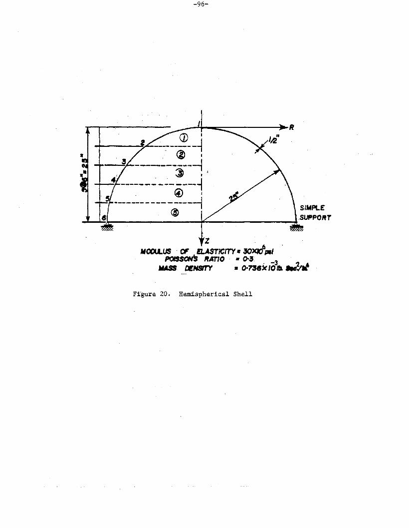
-96-

(j) I

~-i"--j~-~~-----------1

, ~ I

-+--.~I------_-: ------1----------<i~-~

ZMOOCLUS " ELASTICITY. 30xdpal .

POISSONS RATIO . • o-a 3MASS ~N8ITY • o-738j(10 Ib.lIetl:ItI

Figure 20. Hemispherical Shell

Example 3 - FJtee VJ.bJtCLt1.ol1. Ana..ty!.>J.-6 on Empty Wa.:teJt Ta.n.k. wilh SoU

In:teJta.cUon. E66ec.:t.

The tank shown in Fig. 21 was analyzed using seven sixth-order

general elements, the seventh element is the ring footing of the tank.

The soil is modeled with sixteen isoparametric quadratic solid elements.

The soil model is analyzed at a driving frequency of 358.8 rad/sec, the

fundamental frequency of the tank on rigid foundation.

The input data echo of the problem is given in the following page.

The results are presented in the Theoretical Manual.

Week Concrete

Fill • '/l'

Med. Sand

Course Sand

•I

'0 . "0' . 'q . 0 .tt "0:'; ··•• ··0 "p i1 "tJD'IT o'D' :~;"Q: . ,?'o "0'0'~ b --:~ .. ..' tl· D v . .., "/1 0 D· '.,I "0' :'0' 0';":· .,,·.,;.v '·0·: ·'(10. ··.·.<o .•·.·o:.v,". J'.. ...• •.. . ." . .. .....

I

35'" ~ @ ® 16 & Send &G'Q~II

I

104

27'~I

Figure 21. Cylindrical Water Tank on Flexi~le Foundation

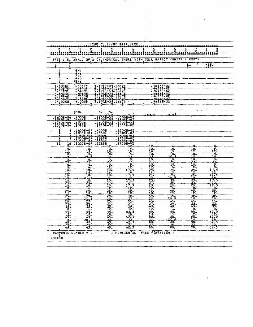
iiHO OF tNPUT DATA DE~K .••••••••••••••••••• • •••••••••••••••••••••••••••••••••••••••••••••••••••••••*.

FREE V IS. MUL. OF ACYL HoIDitlCAL SHELL. WITH SOIL EFFi:CT {UNIiS : I(~FTl

- \ 7 t L 3 1. I.1 0.0Z % 0

7 Ib.O@ 18 .0

-25.-25.

100.. o. 5.~ 1 1 Z7 0

_. C35 e. 8 0.05

.1600E+04 .ftOOOe .3500E-02 .1000E+02--j71H'i +Qft .350QS 3800=-0 Z .15005+02

• 7~OE.04 .3 SOOE .3800E-02 .zoooe+oz.aOOe!! +04 3333i 37501:-02 3500E+02

~ 3 11:100E+04 .4.Q.OOE • HOCe-02

" ft .3 oooe +0" • ZSOOE .4000e-oz5 7 1750e*04 .3 c OOS .3 8 OOi-02

" 8 .2 oooe+o" .33335 • 3750e-020 11 1750S+0" • 3500e .3900e-02

12 lEI .2 OOOE +04 .33335 .3750e-02o. 1:1. 12. 12. 12. 6. a o.o. o. O. 5. 10. 10. 10. 5.

12. 15. 1 a-. lA 18. l5. 12 q.O. o. o. 5. 10. 10. 10. ,.

18 20.5 23. 23. 23. 20 5 18. 18.o. o. o. 5. 10. 10. 10. 5.

23. - 25. 27. 27 27 25. 23. 23o. O. O. S. 10. 10. 10. 5.O. b. 12. 12 12. b 0 O.

10. 10. 10. 17.:5 25. 25. 25. 17.5p. t5• IS' lB. 18. 15. l2. 12o. O. 1 • 17.5 25. 25. lS. 17.51.8. 2(,.5 23. 23. 23. 20 S JS 18.10. ;g. ;~. 17.5 25. 25. 25. 17.523 17 27. 25. 23. 23.10. 10. 10.- 17.5 25. 25. 25. 17.5

------___0.. b. 12. 12 12. 6. o. o.25. 25. 25. 35. itS. 'I'. 45. 35.12 15.- 18 18. 1 flo H. 12 12.25. 25. 25. 35. 45. 45. 45. 3S.18. 2C.5 23. 23 23. 20 5 18 1a.25. 25. 25. 35. 45. 45. 45. 35.23. 25. 27. 27. 27. 25. Z3. 23.25. 25. 25. 3'. -~5. ..5. 45. 35.o. b. 12. 12. 12. o. o. o.

45. 45. 45. oZ.5 80. 80. 80. 02.512. lS. 18. 18. ~ 8. 15. 12. 12.4S. 1t5. 45. 02.5 o. 80. 80. oZ.518. 2G-.-5 23. 1.3. 23 ZC ; 18 1 B.45. itS. 45. oz.5 ao. i!0. 80. OZ.523 25. ZJ' 27. 21 • ,s Z3 23.4'. 45. " . oZ.5 80. ao. 80. oZ.,

1HARr-ONIC NUMBER .. 1 HOR[ ZONTil FREE V IBRATI ON I

1JOeENO

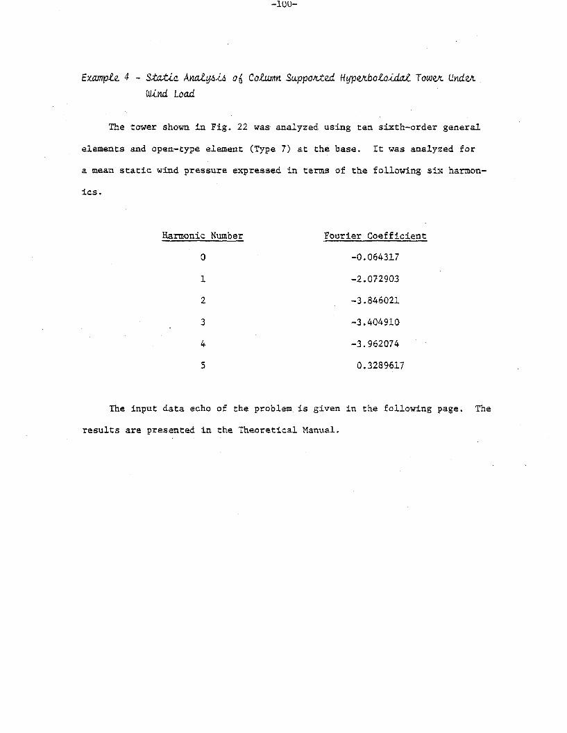
-100-

Example. 4 - S:ta.:tLc. An.a1..Y.6-<A 06 Column Su.ppoJr.:te.d HypeJtbo.R..oJ..da.e. ToweJt UndeJt

Wind Loa.d

The tower shown in Fig. 22 was analyzed using ten sixth-order general

elements and open-type element (Type 7) at the base. It was analyzed for

a mean static wind pressure expressed in terms of the following six harmon-

ies.

Harmonic Number

o

1

2

3

4

5

Fourier Coefficient

-0.064317

-2.072903

-3.846021

-3.404910

-3.962074

0.3289617

The input data echo of the problem, is given in the following page. The

results are presented in the Theoretical Manual.

'. ~C~C OF I~P~T C4T~ C~CK.................................................................** ''0 1. 1 2 Z ; 3 " .. 5 , (: 6 7 7 I

•••• 5•••• 0 •••• ~ ••• ~O •••.• S•••'.J •••• 5 •••.• 0 •••• 5 •••• 0 • •••.5 ••••0 •••• 5 •••• 0 •••• 5 •••• f••••* *.* * ~ •••••••••••••••••*.

. ..__ .•.._--

. .. _-'- - _ - .. -_.-.: __ _-_.,_..•.__ _•.. _-_.:--._-----

1.0.1.• 0.

-_._,.- ........~..... :._....

1

STATlCL1,

~a11

.. WIND. LOACING• '.- Q 1.-_. L lit

WINO l.CACING1. t1 1.~

.WHIO LCACING - ",uJOC1'lIC NtJ~9C:R ,. 2Z 1.1. 14

WtNO LCACINC3. 1.1 14

wtN~ LCACING - HAProtNIC NU~9!R s 4~ 1.

··''-IN6-·LCitiING - JolAQI'CNtC ~u",a=R s 5..__ 5. . L ...

1. 14.J.C.B!Na..

-102-

'0.9'SIZE OF

I.£l.£M£JITS

23-Z CD 36"2 ._._------ 7"

!!HI' (!) .5 -_._.- _._- --

ri)I

® Q3M5

• -------- If

490128' @ '02·(1.....

5 <>--------~

80' ®t\I.,

• . ----_._--I

@50

7 ---- -----50' 0

8 . -_._- ------- ~q»

5/'94' ® §

149-8'

2'083' OIA. COLUMNS

(44 PAfiS)

Z

MODULUS CF ELASTICITY:

5-2XIO' (SHEUJ; 6-4XJo'r.COLSJpsl

POISSON'S RATIO =O·/~

DENSITY=IISO t.lcft -

Figure .22. Discretiz~tion of Hyperboloidal Creek Tower

Exa

mpl

e,5

-V

ynam

ic.

Ana

lyf..

i.606

aF

Ji.e

e-F

ixed

CyU

nciJ

l.ic.

alSh

e.tt

Unde

Jz.

BIM

tLo

ad

As

show

nin

Fig

.23

the.s

hell

isd

iscre

tized

wit

hsix

gen

era

lel

emen

tso

f6

tho

rder.

It

is

anal

yze

dfo

ro

nly

the

zero

eth

har

mo

nic

of

the

bla

st

load

show

nin

Fig

.2

4.

The

Wil

son

-6sc

hem

eis

use

dfo

rd

irect

inte

gra

tio

nan

dth

eti

me

step

ista

ken

as

0.0

00

00

5se

c.

Fo

rC

alco

mp

plo

ttin

go

f

ou

tpu

tth

efi

rst

200

step

sare

specif

ied

for

the

no

rmal

dis

pla

cem

en

tat

the

top

and

meri

dio

nal

mo­

men

tat

the

bo

tto

m.

The

inp

ut

data

ech

oo

fth

ep

rob

lem

isg

iven

bel

ow

.T

here

su

lts

are

pre

sen

ted

and

dis

cu

ssed

inth

eT

heo

reti

cal

Man

ual

.

ECH

OO

FIN

PUT

DA

TAD

ECK

****

****

****

****

****

****

****

****

****

****

****

****

****

****

****

****

****

****

****

****

o1

12

23

3'

44

55

66

77

a..

..5..

..0..

..5..

.•0•..

•5..

..0..

..5..

••

0.•

••5••

.•0.•

•.

5..

.•0••

•.5..

..0..

•.

5..

••

0**

****

****

****

****

****

****

****

****

****

****

****

****

****

****

****

****

****

****

****

**A

NA

LY

SIS'

OF

FRE

E-F

IXE

DC

YLI

ND

RIC

1\L

SHEL

Li(

6th

ORD

EREL

El-lE

NTS

)4

6

-H

ARM

ON

ICN

UM

BE

R;

a(U

NIT

;PS

I)*

N.I.

SCH

EM

E:W

ILSO

N1S

I f­ C v I

,Out

put

CoY

Ww

lC

Md

T-im

eH

i.6to

Ji.y

Out

put

Con

:tAol

CaJi.

d

Veg

Ji.e

u06

FJi.e

edom

CaJi.

M

MM

f..M

atJU

xCa

Ji.d

Vyn

amic

.Lo

adTy

peCa

Ji.d

Load

TUle

CaJi.

dLo

adin

gC

ontn

olCa

Ji.d

Vi.6

tJU

bute

dLo

adin

gC

aJtM

ViJ

l.ec.

t1n

tegJ

i.aU

onSc

.he.

me

CaJi.

d2

Va.

taCa

Ji.d

60Ji.

Vyn

amic

.An

alyl

.>,u

,In

itia

lC

ondi

tion

CaJi.

dT-

ime

Ste

pC

ontn

olCa

JtdT

Ule

CaJi.

dn0

Ji.In

pu

tT-

ime

Fun

ctio

nRec.oJi.dPoi~

CaJtd

12

00

1.0

-9.2

1.0

-9.2

1

-8.6

27

75

6-7

.14

56

37

-7.1

45

63

7-7

.77

21

57

0.9

58

18

45

10.0

02

4E

-l0

.00

24

E-l

66

1 13

111

1.0

1

FOR

HA

RMO

NIC

NU

MBE

R;

00

.00

00

05

1.0

0.0

01

LOA

DIN

G2 6 7

1 320 2

BLA

ST a 1 6 2

TIM

EH

ISTO

RY

61

11

61

10

.07

22

.51

1,1

11

10.1

000E

OO

O.I

OO

OE

OO

l.05

00E

070.

3000

EO

O60

.100

0EO

OO

.100

0EO

Ol.

0500

E07

0.30

00E

OO

66

66

66

66

O.0

00

00

53

BLA

STLO

AD

ING

0.0

0.0

JOB

END

-104-

9-e"

22'S'

oi"

~- -----. ~ I

3 ----------1~ I

----------~Q) ,

5 ----- ----~@ I

------ -- --I~ -I.

I ~_+-----__---r-"" "2

+5'

z

MOCllJJS ex: ELASTICITY:: lOex I06ptl

PO/sse"s RATIO :: 0-3MASS t:eISlTY :: 2-4Xit lb. S«;'2;ln4

Figure 23. Fixed Base Cylindrical Shell

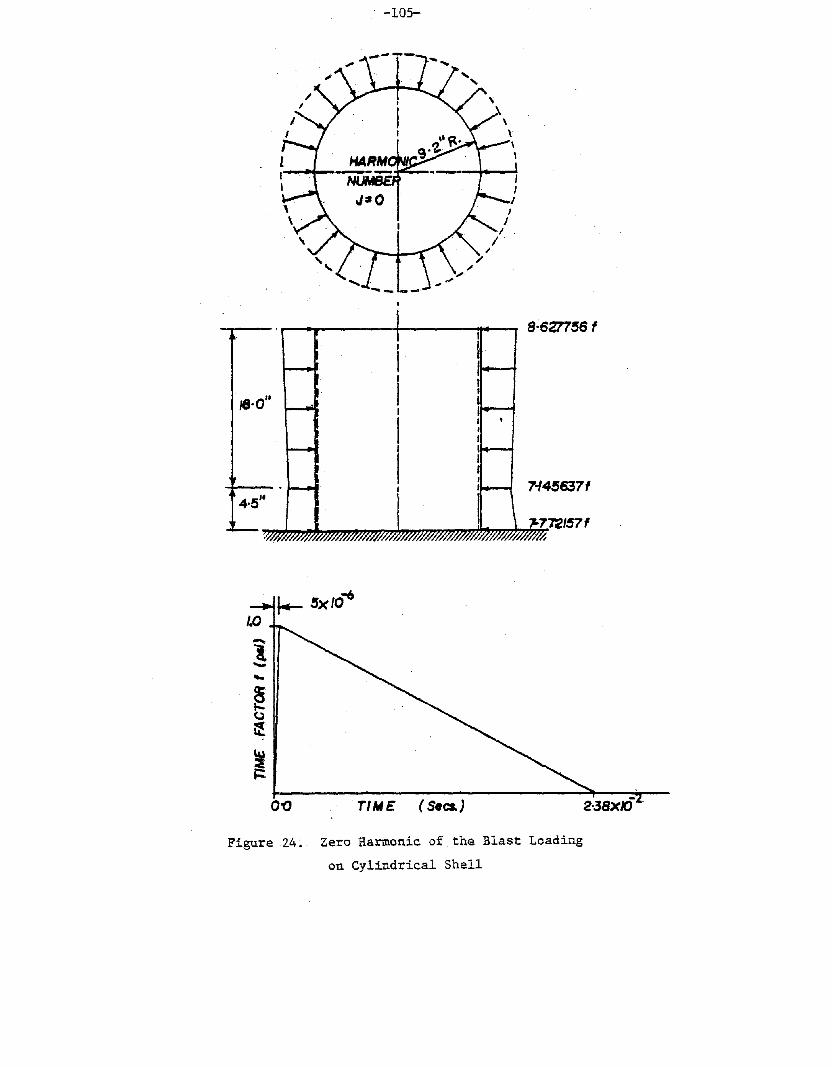
18·0"

-105-

II

JI

II

/.-'"~,...

""4~637f

-1.-....~(,)~.

~0'0 TIME (Secs.)

Figure24~ Zero Harmonic of the Blast Loading

on Cylindrical Shell

-106-

Ex,ampl.e. 6 - HypeJtbol.o.i.da.e. Shell. UndeJt Dynamic. Woo Load

The tower of Fig. 22 is analyzed for the wind loading, digitized at

0.5 sec. internal, shown in Fig. 25. This analysis was preceded by a free

vibration analysis to determine..the damping coefficients (~ = 0.276, B =

0.0058) and to select the time step (~t = 0.025 sec.). The pressure was

assumed constant over the height of the tower and eight harmonics were used.

The input data echo for the problem is given in the follOWing page. It may

be noted that the control card for dynamic analysis for direct integration,

data card for dynamic analysis, and the record points cards are provided

for the first harmonic only. Accordingly the columns 30-35 and 36-40 of

the problem control card were left blank. The results are presented and

discussed in the Theoretical Manual.

-...L.V/-

SM

.l.A

TE

DR

ISE

BA

SE

DO

N-

MTA

.FO

RS

TAT'

ION

NO

.13

64

52

-'6

0tJ

8tJ

6

(AFT

ERSP

LiNE

FIT

TN

i)

52

.>

"5

0

TIM

E1.

0

~0

8~ I

f/

06

/::J

HARM~

NO

FQ.fl

IER

CO

EFF.

·I

.q:

/0

-0.0

66

22

~~

,-2

.19

86

.0·

"/ I

•-4

.07

93

'I

!~

-3.

611t

Jl..

~l

c..

-0

.42

02

4c

II

/e

0.3

46

92

Q.2

IS0

.14

74

6

~I

..7

O.l

67

H

ElA

PS

ED

TIld

E(S

ect.

J

Fig

ure

25.

Tim

eH

isto

ryo

fW

ind

Loa

ding

for

Hy

per

bo

loid

alT

ower

Example 7 - Reoponoe Spewwm AnalqJ.>AA on HqpeJtbolo-<.da1. Shell. Wilh

Soil rn.:teJta.cUon..

The tower shown in Fig. 26 is analyzed under the ground motion

given by the response spectrum of Fig. 2]. The damping ratios for both

the shell and the soil 'is 5% of <he critical damping ratio. The analysis

of the soil is carried out under driving frequency of 20 rad/sec. The

soil medium is an elastic half space with shear modulus of 1600 k/sq.

ft. and Poisson's. ratio of 0.4. The input data echo for the problem is

given in page (112). The results are presented and discussed in the

Theoretical Manual.

-lJ.U-

:p (13.62)( 0.001 Fl

• (60.12)

T {A20.00}

y (580·37)

C0L148"'cj>80 DrAG.

----__ r

9 I ! -120j-I I I I__________J. . __....-~------_

I I I I

I : SOIL MEDIUff\

,

I, I.I I I t------------I--f--rT---------I 1 I

Z

=-~ CD

I,--I G~.----4I

UoIZ

-0u

Figure 26. Cooling Tower on a HypotheticalFoundation

-.1..1..1.-

10.01.00.100.01 "--......--1--l....l....l.::..l....l.J"l,__~..J-..I..~looU...l.l.._-..l._~..l-l..A.I..l.Io'

0.01

>-

~~

~~~ O.la\---+----~-l__-~---~-I__~~---~__tI

~~

UNDAMPED NATURAL PERIOD (SEC.)

HORIZONTAL [0.20 9 .5% Damping]

Figure 27. Horizontal Re~ponse Spectrum

. /'

"'.

':.'.

to

.'

.--

\~:

".i

1'(

\

EiH

OO

FIN

PU

TD

ATA

DEC

Ki

,~

*************.*******.~***.*********••

*~**¥*******.***~*****.*****~*************

o1

"'-

'C

22

,3'

,34

.4

5--

5--

;--'

6~--7-'

-78

••••

:>••

•'.

0.~

~.5

••••

0••••

5••

;,.

0·•

•••

5••••

0••••

5••••

0••••

5••••

0•••

~~

....

..0

••••

5••••

0**

***I

f.***

***.

''***

****

****

****

****

*'***

****

****

****

****

'Ii*-*

*",**

***.

***.

.....*

****

****

*.

,....

','

.".

..

'.'..

......

,"

.:..

':',

''.

..

'.'

."

..'

,.....

.'.

'.'

.

TE

ST

.PR

OB

LE

M'

(,R

ES

PC

JN

SE

'SP

EC

TR

UM

AN

AL

YS

IS)

.~.

BA

SEw

ITH

E.a

.S.

'9l'

'3

3'

·1:

1,\

10

1.

i,'

..

1;2

3.6

H3

77

-27

58

1.5

16

51

53

6ff

40

.5'3

7-,

-,-~,

.'4

'1

a-1

.);.'

9.4

()l

53

-L302~5923225462.8a292

,7'

10

."j'

.29

99

99

78

04

-:-1

'.8~2TT168-2

ti8

01

70

.".2

99

99

97

80

4-1

.'tH

.21

11

68

2I)'.

.1

01

-1

60

.37

2-.

29

'19

99

78

04

-.1

!OaT

.'2

,n6

l:f2

.4o.

----

--.-

-.-~

--

T'"

ai3

59

.8

80

,.

,.

""

,9

'4

06

.38

0'

---------;~

----

..----~

..'

,~

10

:'420~000

','.

11~333Er.000E

'o.1

91

E-t-

05

.16

67

Ed

,.4

1b

bE

'.If

,65

8E

02

---~

2'

.aO

OE

.6b

6lE

5~191E:

...·(

)5.1

66

71

::.4

16

6E

.46

58

E-0

2/

•~667E',

.66

67

£5

.19

1E

"'0

5.1

66

7£

'.4

16

6E

.46

58

E-0

2t

5.

66

67

t:.I;

.6'3

1Q

E5~19tl;t-Q5.1667E\

.41

66

E.4

65

8E

-02

\'6~8JTo~~S80E

5;1

9fE

+(f

5.1

66

7'E

,4

16

6E

·,.4

b5

8E

-0

2I

','

7.9

58

0E

3.5

00

E5

.19

1E

+0

5.1

66

7E

41

66

E~4658E-02'

J'

'81

2.S

7E

25

.1,4

E5~604E+0512.57E

e.S

7E

.46

58

E-0

24

.00

0e,

4~OOOE'

~)667·

94

.90

0E

20

.00

E5

..1

91

E+

95

.l6

67

E,...

41

6b

E.4

65

8E

..,.

02

\..

/

1uv

...,

\3

,I

u·.

,J.

,.",

'"J

iI

r~'

20

.7

'----

--7

5.-~-~":"'.'Z

!lp:r.-

=,.-:-.---llor;.=-iUrr!'i5'---~-----:----:-~-:--"""'--'----------~-----'

.lb

OQ

Et-

04

.-.4

00

0E

tOO

.3

50

0E

-0

2·;

"'

I'

,I

"

HA

kM

ON

IC

NU

MB

ER

=1

Rep

rod

uce

dfr

om1

,.'

1'

best

avai

lab

leco

py

.

1".0

5,2

.05

3.~05

3'\

31"

.:s3

33

.33

.3

3'

,"3

31

I'9

'.04

9.0

7'

9.09~~5

1.3

33

30

.66

67

0.9

5,8

,4

.09

0.0

i.•

.•..

"'.•

'I'

:oJ-I

IHO

RIZ

ON

IAL

RE

SP

ON

SE

~PECIRUM)

S'M

MP

·O.0

5U

AM

PIN

GIS

SE

Jl'

6,'

,'1

".

""'.

,,

.05

\".,/

J,.

"i.

f'I

,."

,'

,IO

O·.

oaO

Oi·

,.0

10

33

.33

33

'.0

32

;/7

.81

25

.35

0'

2.5

00

Q1

.10

0•

22

73

1.

10

0•I.

46

5J

OB

EN

D"'.

,'

,\

I

,('

,"'

'.

Example. 8 - Tune. H-<.otOJl.y AVIP.1..y~-<.o on HYPeJl.boloJ..da1. Shell

a.. WUh Soil Enne.e.:tb. WUhotLt Soil Enne.a

The tower of Fig. 26 is analyzed under El-Centro Earthquake

(5-18-1940) EW Compo The soil medium is considered as elastic half

space as in Example 7 and then the analysis repeated with fixed lower

boundary at node #10. The time of the analysis is taken as five seconds

and the time step for Newmark S method integration is taken 0.02 second

in case a (soil-structure interaction) and 0.005 second in case b (fixed

base). Th~ damping coefficients (a=O.7l5779 and S=0.003356) are obtained

based on 5% damping ratio for the first two modes of vibration (the

modes of vibrations are obtained in Example 7). The input data echo

for the problem is given ,in the next two pages. Fig. 28 shows the plot

of M~ at node #7 (6=0°) for the soil-structure interaction case (case

a). The rest of the results are presented in the Theoretical Manual.

eCtl<... 01' Ilql''JT· ~Aj ..... DECK**.*******•••*~********~**••*.4*.***••*.*.*****••~~**••****~***.******.**.*****.o It!: t' :l 21 4 4 J j ,6 () "f ., a

****'4********.********************.****.*.***.*.4***.**••••••*.**••*.*••~ ••****Tl,~\! R[STOA:, ANAL. lCOOL1NG Telae'" atTh :::lOlL: 1IiTePtAt:T10N, Ct: ClhTFlO eN

, ,,1 40 3 l'1 1 04 1 0

1 ad 8017 0:; 1 v

=x •.-1. 9.400153' -130a,.5923225400Z .<laZ92

.299999,604 =1. 67.2111582

.299Q997804 -1. 87.2111b82

.299999,a04 -1.81.2111602-160.-372

4 o.8 359.080

21.000E .oo67c3.060iE .CObIE ,

4_000e .100'

.40seeoz

.4"58E-02

.40:;61: 024.0001:

.4058E''02

.40~ae::a02

'.405SE-023

5

,4-1eoE.4100E

.410-62

.41bOe

.41boe

.41o"E12:.'HI:

"

S.191E.05.16o.7E

5ol91e;.o5.1007EJ ad04E • ,jj t!:." , E

5.191E.05.1607E).191E+O'.160'E5 • 19 1 e; +<>5 • 1067 E;;.1 ~leFO;;.16b"E

'5.I91e+O!J.l061!

3Z31432

tj 406.35010 4020.000

lE.J3SE i.OOO~

7.YSdOE 3.S00Eal •• J"fE !J.14e"4.000E 20.00E

J , 21 :3

.05

250

5 sec.0.22310 0.08 0.09514O.ZiZ'l 0.10 O.173ea0.4;;963 0.240 0.40662o .45t1:35 0,_5£ a_160?60.79724 0.400 0.436.J5O.Jlltli e ...a e.2"ftlB"f0.271:l1:l7 0.56 0.43307e.t17S ..6 e064 El .. Ell;Z02Cl.340t19 0.72 0.42979a. ~ 95 rot a.SEl t.eaZb5

-1.72244 O.dS -1.36155l.66b60 0_!>6 1_61664

-1.63386 1.04 -1 .. 80446101,3166 lile a.US6..

-0.69882 1.20 -0.154201.JdZa~_ .l.za. O.61oao

>-3.17585 ' 1.36 -3.60893',-3.277'56; 1.44 -3.07087'-3.97960-' '1.52- -3'.60565' '-,-1.2467, 1.60 -\1.50853

1.96522 1.68 2.7395040.87205 1.76 3.910763.54003 I.S4 2.70341

-4.85893 1.92 -5.85956-40.99016 2.00 -40.74410-3.d68l1 Z.08 -3.56956-1.95210 2.16 -0.31168

2.32623 2.24 1.91929_ -2.21457 2.32 -2.70998

O.Z4C!,d 2.40 1. 466543.02494 2.408 2.542650.000::3 9 z.se -2.00161

-0.1201-67 2.64- 0.931763.O:3a:;~ 2.12 2.135630.47244 2.00 1.08268;).22310 2.d8 5.a39902.58530 2.96 1.069552.Z63iS 3.-04 2,.332661.77822 3.12 1.709322.65143 3.20 1.41404

tg:;~ci:~3.28 -0.02297:3.36 a .. a8386

0.04961 3.44 1.40748J. 1 0368 J.S2 J ':35821

-~.03806 3.00 -3.12664-2.02400 3.08 -Z.42162-1.233bO 3.76 -0.78701-0-0.06102 3.04 -t.36£23-0.90879 3.92 -0.21325-1.::J3S;O 4.00 -1.di006

0.67257 4.08 0.685701.5813, 4.16 -5.12;96

-2.20801 4.24 ..'0.1339903.3~::S02 4.:52 J.3CS5962.10864 4.40 1.715882.32023 4.43 2:.6~10?)

-3.55.J15 4.56 -3.051183.,3 ~J{)f q;.04 3.:JIO'l3

-3.60470 4-.72 -2.06746~.OTd'l'4 "~O 1.437'022.26:.37.3 ~ .. (j8 2.20 ..01a. Ob6gJ 4.95 1.12:Z44

. I

20.25.

h 2501 •

(HORIZCJQiAC GRLQNO MOrION)

• 5.003350

t· • zs.710779

j

1, 225.7

MAkICiCNI.C jQU,CJibER 1

-115-

~~HO OF I~PUT OATA 0~~K .*~***•••••*••*•••~*.****.*.¥.***••~.***.~~.~.*~~*.*••••*.**~*••••*••*.*••**.****

o I I .!. ~ .3 .3 ,. " 5 ;; .. Q 7 7 <l•••• 6 •••• J •••• 5 •••• ~ •••• 5 •••• J •• ,.5 •••• J •••• ~ •••• J ••••a·"·Q·,··~·,•• Q ••••5 •• t.q".*.,,*•.**.**..*..,***.*...*******-..* ...--.**,*~.*~*,*.*~.*.**,,*••••••**••"'••*.....*...**.........

1 0I _t 60 • .372

n/olf; HISTORY9 1

..Z9999978u4 - 1. ':'7 ••U 1 lo..~.29~9Y9lBQ4 _1. 8Z~2111baa

-1.-l.

ANAt. •. 'COOl-LNG Tu ..eR iii TH F IXEO cA::iC;;9. J

1 01 qI 0

R017 117

"

1..

" O.d 352.8899 400.380

10 4?O.OOO11.333a l.uQue21.QQQt; .bpOZE3,OQo7~ .ooolE:5,6667¥; .831 JE

. 1 1 1

.5 .191!1;?u5.1 06 7E5.1911;+05.1067\;;,

.4looE

."lgDEe40looe:• '40·1 obE..... looi!.4JboE:

.4058e::-02

.46sac:-y2'''058e-0~.*05dE-02.4Q.QO~-'l.a

.4o5dE-O.i:!<hoooe .1007

.j .3 . .jI

1.3 5

31

.3 -'I

5

j .

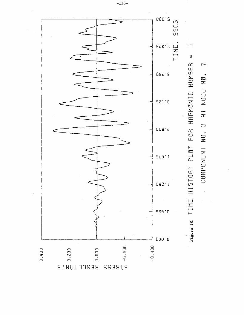
-116-

000"5(f)

UW(f)

~SL£"h w~1--1 1/I-

a: r-w

OSL"£ CD2: 0:::::J ZZ

UW0

1--1 0521 'S Z Z0:2: I-a: a::a::I

(I)

005"2 a: •0 0l..L. Z

l- I-0 z

5L9' ! -l W(l.- z'

0>- (l.-IT: ::E0 0I- U052'1 ())1--1

:r:

W::E-529'0 I-

00N

(l)~::lOJ)

000"0 .,..j

~

0 00 0 0 0 00 0 0 (\J ::::I"::::I" (\J 0 "

,. , , 0 00 0 .0 1 I

SlNCJllnS3tl SS381S

-117-

REFERENCES

1. Gupta, K.K., "Eigenvalue Solution by a Combined Sturm Sequence and

Inverse Iteration Technique", Int. J. num. Meth. Engng., Vol. 7,

1973, pp. 17-42.

2. Basu, P.K. and Gould, P.L., "SHORE-III Shell of Revolution Finite

Element Program - Static Case - Theoretical Manual, Research Report

No. 41; Users' Manual, Research Report No. 42, Structural Div.

Dept. of Civil Engineering, Washington University, March, 1975.

3. Sen, S.K. and Gould, P.L., "Free Vibration of Shells of Revolution

Using FEM", J. Engng., Mech. Div. ASCE, Vol. 100, No. EM2, Apr:f,l,

1974, pp. 283-303.

4. Basu, P.K., "Dynamic and Nonlinear Analysis of Shells of Revolution",

Doctoral Dissertation, Washington University, St. Louis, Missouri,

1977 •

5. Basu, P.K. and Gould, P.L., "SHORE-III Shell of Revolution Finite

Element Program - Theoret~cal Manual", Research Report No. 48,

"Users' Manual", Research Report No. 49, Structural Div., Dept.

of Civil Engrg., Washington University, Sept. 1977.

6. El-Shafee, a.M. and Gould, P.L., "Analytical Method for Determining

Seismic Response of Cooling Towers on Footing Foundation", Research

Report No. 55, Structural Div., Dept. of Civil Engrg., Washington

University, Sept. 1979.