The Influence of Void Size on the Micropolar Constitutive Properties of Model Heterogeneous Materials

A. Waseem, A. J. Beveridge, M. A. Wheel & D. H. Nash

Department of Mechanical Engineering,

University of Strathclyde,

Glasgow, UK, G1 1XJ

marcus.wheel@strath.ac.uk

Tel +44 141 548 3307

Fax +44 141 552 5105

Abstract In this paper the mechanical behaviour of model heterogeneous materials consisting of regular periodic arrays of circular voids within a polymeric matrix is investigated. Circular ring samples of the materials were fabricated by machining the voids into commercially available polymer sheet. Ring samples of differing sizes but similar geometries were loaded using mechanical testing equipment. Sample stiffness was found to depend on sample size with stiffness increasing as size reduced. The periodic nature of the void arrays also facilitated detailed finite element analysis of each sample. The results obtained by analysis substantiate the observed dependence of stiffness on size. Classical elasticity theory does not acknowledge this size effect but more generalized elasticity theories do predict it. Micropolar elasticity theory has therefore been used to interpret the sample stiffness data and identify constitutive properties. Modulus values for the model materials have been quantified. Values of two additional constitutive properties, the characteristic length and the coupling number, which are present within micropolar elasticity but absent from its classic counterpart have also been determined. The dependence of these additional properties on void size has been investigated and characteristic length values compared to the length scales inherent within the structure of the model materials. Keywords:- micropolar elasticity; Cosserat elasticity; heterogeneous material; size effect 1. Introduction In a homogeneous material any variation from one point to another that may be present in the constituent structure is regarded as inconsequential in determining mechanical behaviour when loaded because the size scale associated with structural dissimilarity is negligible. The behaviour is then usually described by a constitutive theory such as classical or Cauchy

elasticity (Sadd, 2005) which can be employed to determine the resulting deformation due to applied loading at all size scales of interest. Central to such a theory is the notion of locality; the state of stress at a particular point is uniquely related to the strain there by the constitutive theory, hence the theory is applicable at all scales. Conversely, in a heterogeneous material variation within the structure may influence mechanical behaviour. For example, material samples of the same geometry but different sizes may have different stiffnesses, a size effect that is not forecast by classical elasticity theory but is acknowledged by other more general theories. Other consequences of heterogeneity include changes to local stress fields around discontinuities and defects and alterations in the propagation of elastic waves. Ordinarily, more general elasticity theories recognise material heterogeneity and the resulting nonlocal dependence of stress on strain in one of two distinct ways; either through the introduction of higher order stress or strain gradients in the constitutive relations or via the incorporation of additional independent degrees of freedom. The first approach is exemplified by gradient elasticity theories (Maugin and Metrikine, 2010) while micropolar or Cosserat (Eringen, 1966; Nowacki, 1972; Eringen, 1999; Sadd, 2005; Maugin and Metrikine, 2010) and micromorphic (Eringen, 1999) elasticity are examples of the second. A common feature of all generalized elasticity theories is the inclusion of additional constitutive parameters or properties within the constitutive relations. These parameters will of course be material dependent and, for a given material, will ultimately have to be identified by experimentation. Almost ubiquitous among these additional properties is the material length scale, a parameter that establishes nonlocal dependencies and reflects the size scale of the underlying material structure. Recent theoretical work (Bigoni and Drugan, 2007) clarifies the motivation for generalized elasticity theories: homogenization of the response of a heterogeneous material comprised of a relatively dilute periodic distribution of regularly shaped voids in a classically elastic matrix is shown to be equivalent to micropolar elastic behaviour implying that this description of the material avoids the need to consider local strain gradients and stress concentrations around heterogeneities in any detail. Identifying the additional constitutive properties of heterogeneous materials experimentally is a challenging task since the customary approach involves loading material samples of similar geometry but differing sizes. Any observed dependence of stiffness on sample size can then be compared to an analytical or numerical prediction of the size effect and the relevant property inferred from the comparison. An early attempt (Gauthier, 1981) to exploit this size effect based approach to identify the additional micropolar constitutive properties of a model material formed by encapsulating aluminium shot within an epoxy matrix proved inconclusive; the anticipated increase in stiffness with reducing sample size was difficult to identify from the data which displayed significant scatter. However, subsequent attempts to detect the size effect in both synthetic (Lakes 1983; Lakes 1986; Anderson and Lakes, 1994; Lakes, 1995) and biological materials (Yang and Lakes,1982) have been more successful and constitutive data have been obtained from the observed effect. Nevertheless, the length scales associated with the heterogeneity in these materials preclude the use of conventional mechanical methods of loading the necessarily small samples so a sophisticated electromagnetic loading technique was used instead. Careful surface preparation of the samples (Anderson and Lakes 1994) was also identified as a necessary requirement in obtaining consistent data. Just recently experimental testing and FE modelling of another model heterogeneous material yielded a size dependence on stiffness consistent with micropolar elasticity theory (Beveridge et al., 2013). The material comprised of a regular array of circular perforations or voids

machined into aluminium plate and it was designed specifically to investigate the effect of material structure on mechanical behaviour by experiment and by FE analysis. The additional constitutive properties present within micropolar elasticity theory but not in its classical counterpart were quantified by comparing the size effect obtained from experiment and corroborated by FE analysis with analytical and numerical predictions. Perhaps the most noteworthy result was the remarkable similarity between the characteristic length identified by this approach and the dimensions defining the heterogeneous structure of the material. While the deliberate creation, testing and analysis of a model material may appear contrived it does provide a straightforward means of determining the influence of the underlying structure, specifically the void volume fraction and distribution, on the constitutive properties. In addition, the heterogeneity can be introduced into the material at a size scale suitable for testing on whatever loading equipment is available. As already mentioned, testing a real material may require bespoke equipment. Deliberately introducing the voids in a regular array also facilitates FE analysis of an entire test sample thus providing a means of substantiating experimental data as required and in due course supplanting the need for extensive experimentation. Finally, the model material provides some basis for comparison with the theoretical predictions of constitutive behaviour obtained by micromechanical analyses of the type thoroughly reviewed previously (Ostoja-Starzewski, 2002). Typically such analyses represent the material structure as a lattice of interconnected elements. The constitutive properties are then usually deduced by considering the behaviour of a small portion of the lattice. This approach has seen some success in explaining the behaviour of real materials with regular honeycomb like structures (Gibson and Ashby, 1997). The present work builds upon this recent activity by seeking to determine how variations in the underlying structure of the model material influence the effect of sample size on stiffness and thereby the associated micropolar constitutive properties. This work concentrates on variations in structure achieved by maintaining the array geometry and altering the void size alone. In addition, three further developments are considered in this work; the sample geometry is changed from straight beams to circular rings, the matrix material is changed from aluminium to an acrylic polymer and the size scale of the heterogeneity introduced into the samples is reduced. In advance of describing the design, manufacture, testing and analysis of the samples the development of an analytical solution for the deflection of a slender circular ring of micropolar material loaded diametrically is presented. The derivation of this solution originates from plane micropolar elasticity theory which is also briefly summarised. 2.0 Deflection of A Slender Diametrically Loaded Micropolar Ring In a two dimensional micropolar material the strains, εxx, εyy, εyx, and εxy, are related to the displacement components, ux and uy, and the microrotation, φz by (Nakamura and Lakes, 1995):-

−+

=

zxy

zyx

yy

xx

xy

yx

yy

xx

uu

uu

φφ

εεεε

,

,

,

,

(1)

while the force stresses, τxx, τyy, τyx, and τxy, and couple stresses, mxz and myz, are related to the strains and curvatures, φz,x and φz,y, by:-

( ) ( )

( ) ( )

++

+++++

+++

+++

+++++

=

∗∗

∗∗

yz

xz

yx

xy

yy

xx

yz

xz

yx

xy

yy

xx

mm

,

,

*

**

*

*

*

*

*

**

000000000000000000

00002

)2)(22(2

)2(

00002

)2(2

)2)(22(

φφεεεε

γγ

κµµµκµ

κµλκµκµλ

κµλκµλ

κµλκµλ

κµλκµκµλ

ττττ

(2)

The presence of additional couple stresses acting on a material element, shown previously (Beveridge et al., 2013), implies that the shear stresses need no longer be complementary since any imbalance can be compensated for by the couple stresses. The modulus λ governs dilatational deformation, while μ* and κ together govern distortional deformation. Furthermore, κ governs additional deformation resulting from the difference between the conventional macrorotation, θz (= uy,x – ux,y), and the microrotation. The constants λ, μ* and κ can be recast in terms of the engineering constants EM and νM corresponding to Young’s modulus and Poisson’s ratio, a characteristic length, lb, and a coupling number, N (Lakes, 1995). The constitutive equations, (2), thus become:-

( )

( )( )

( )( )( )

( )( )( )

( )( )

( )( )

−−

−−

−−−

−−−

−−

−=

yz

xz

yx

xy

yy

xx

Mb

Mb

MM

MM

M

M

M

M

yz

xz

yx

xy

yy

xx

ll

NNN

NN

NE

mm

,

,

2

2

22

2

2

2

2

2

12000000120000

00121

12211

00

0012

211121

00

0000100001

1

φφεεεε

νν

νν

ννν

ν

νττττ

(3) The subscript M is added to the first two of these engineering constants to distinguish them from their classical elasticity counterparts. The characteristic length determines the domain size influencing the couple stresses at a point and is thus expected to reflect the intrinsic length scales associated with the structure of the material. The coupling number quantifies the disparity in the shear stresses and thereby characterises the degree of micropolarity exhibited by the material. The lower bound occurs when N = 0 and corresponds to classical elasticity while the upper bound when N = 1 is termed couple stress elasticity (Lakes, 1995; Eringen, 1999). As illustrated previously (Beveridge et al., 2013), the microrotation is associated with the skew symmetric part of the shear stresses, τa [=1/2(τxy – τyx)], while the conventional macrorotation is associated with symmetric part of the shear stress, τs [=1/2(τxy + τyx)].

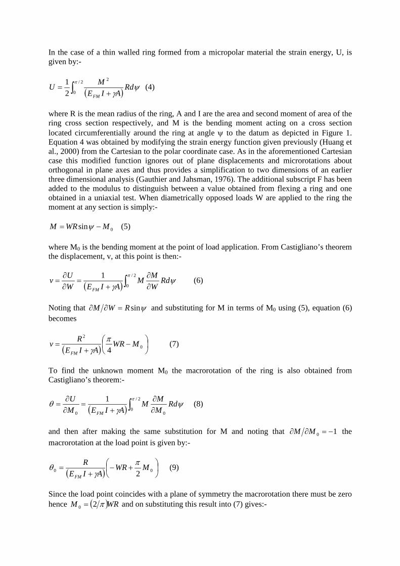
In the case of a thin walled ring formed from a micropolar material the strain energy, U, is given by:-

( )∫ +=

2/

0

2

21 π

ψγ

RdAIE

MUFM

(4)

where R is the mean radius of the ring, A and I are the area and second moment of area of the ring cross section respectively, and M is the bending moment acting on a cross section located circumferentially around the ring at angle ψ to the datum as depicted in Figure 1. Equation 4 was obtained by modifying the strain energy function given previously (Huang et al., 2000) from the Cartesian to the polar coordinate case. As in the aforementioned Cartesian case this modified function ignores out of plane displacements and microrotations about orthogonal in plane axes and thus provides a simplification to two dimensions of an earlier three dimensional analysis (Gauthier and Jahsman, 1976). The additional subscript F has been added to the modulus to distinguish between a value obtained from flexing a ring and one obtained in a uniaxial test. When diametrically opposed loads W are applied to the ring the moment at any section is simply:-

0sin MWRM −= ψ (5) where M0 is the bending moment at the point of load application. From Castigliano’s theorem the displacement, v, at this point is then:-

( ) ∫ ∂∂

+=

∂∂

=2/

0

1 πψ

γRd

WMM

AIEWUv

FM

(6)

Noting that ψsinRWM =∂∂ and substituting for M in terms of M0 using (5), equation (6) becomes

( )

−

+= 0

2

4MWR

AIERv

FM

πγ

(7)

To find the unknown moment M0 the macrorotation of the ring is also obtained from Castigliano’s theorem:-

( ) ∫ ∂∂

+=

∂∂

=2/

000

1 πψ

γθ Rd

MMM

AIEMU

FM

(8)

and then after making the same substitution for M and noting that 10 −=∂∂ MM the macrorotation at the load point is given by:-

( )

+−

+= 00 2

MWRAIE

R

FM

πγ

θ (9)

Since the load point coincides with a plane of symmetry the macrorotation there must be zero hence ( )WRM π20 = and on substituting this result into (7) gives:-

( )

−+

=π

πγ 4

823

AIEWRv

FM

(10)

If the ring cross sectional thickness, t, is the difference between the outer and inner radii, denoted Ro and Ri in figure 1, while the breadth, b, is the transverse dimension of the section then given that for a rectangular cross section btA = and 123btI = , equation (10) can be rearranged to give the stiffness, K, of the ring as:-

( )

+

−=

23

2 183 t

lRtbEK bFM

ππ (11)

where the characteristic length in bending, lb, is defined as:-

FMb E

l γ12= (12)

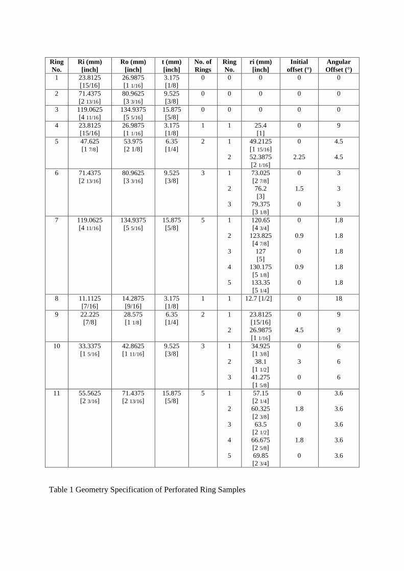
Equation (11) can be regarded as the expression for the stiffness of a classically elastic slender ring (Sturmath et al., 1993) corrected by an additional term, given in the square brackets, to account for size dependency. By analogy with recent work (Beveridge et al., 2013) equation (11) can be used to determine both the flexural modulus and characteristic length of a micropolar material by finding, on this occasion, the stiffness of slender ring samples of different radii but the same breadth and aspect ratio, R/t. Any variation in stiffness with the reciprocal of thickness squared, (1/t2), can then be identified and for a micropolar material this variation should be linear. In this case the flexural modulus and characteristic length can be found from the intercept of the linear variation with the stiffness axis and its gradient respectively. In the case of a classically elastic material the characteristic length is negligible so stiffness should be independent of size and consequently the gradient of the stiffness variation will be zero. Recent work confirmed that straight beams of a model material loaded in three point bending did indeed exhibit behaviour consistent with micropolar elasticity theory. In the present work a similar model micropolar material is utilized. The material possesses the benefits that the size scale and regularity of its constituent structure facilitate testing on available equipment and FE analysis of an entire sample respectively. The ring samples use in the present work offer the additional benefits of a more compact geometry than beam samples and a more straightforward loading mode. In the beam samples investigated recently these two factors necessitated careful consideration of support flexibility in order to obtain reliable stiffness data from which constitutive property data could be derived by the approach outlined. 3. Ring Samples: Design, Manufacture, FE Representation and Mechanical Testing Sample Design Figure 1 also shows the geometry of a generic ring sample. For each individual sample the inner and outer radii, Ri and Ro are listed in Table I which records these dimensions in metric

units with their imperial equivalent in parenthesis; the latter being used for convenience during manufacture. The ring thickness, t, is then the difference between Ro and Ri. The first three samples listed in the table were left unperforated. The stiffness data obtained from testing these three samples could then be used to determine the modulus of the acrylic polymer that constituted the matrix material in the remaining, perforated samples. Although the mean radius, (Ri+Ro)/2, of each of these three samples differed significantly they are all geometrically similar; they all have an aspect ratio of 8 where the aspect ratio is now defined more precisely as the ratio of mean radius to thickness, (Ri+Ro)/(2t). The next four sample geometries listed in Table 1 also have varying mean radii but the same aspect ratio of 8. However, in these geometries perforations are introduced into the samples with the number of concentric bands of voids depending on the mean radius and thickness of the sample. The illustrated initial offset from the datum of the first void in each band is listed in the table as is the the offset angle between successive voids within a given band. The geometric details listed were selected to produce a triangular array of perforations within each ring sample as shown with the void separations remaining fixed across all samples An equilateral triangular array is ideally sought but inevitably the circumferential separation between consecutive voids varies from one band to the next. However, given the overall size of the samples this variation is not excessive. For each of the geometries samples with perforation diameters of 1.588 mm (1/16”), 1.984 mm (5/64”) and 2.381 mm (3/32”) were manufactured giving a total of twelve perforated samples with an aspect ratio of 8. The remaining four geometries detailed in Table 1 once again have a variety of mean radii but a common aspect ratio of 4. The offset angles were adjusted so that the circumferential separations between consecutive voids correspond to those in the samples with an aspect ratio of 8 thus ensuring that in all samples the perforation arrays match. Once again for each sample geometry perforations of the same three diameters were produced giving a further twelve samples each having an aspect ratio of 4. Sample Manufacture All samples were manufactured from stock 6 mm Altuglas® acrylic sheet using a computer numerically controlled (CNC) milling machine. For each of the perforated samples the array of voids of the required diameter was first drilled into the virgin sheet. The sheet material located inside the inner radius of each sample was then removed in a continuous circumferential cut and finally the sample itself removed from the remaining sheet in a second circumferential cutting operation. The perforations were machined before cutting the sample from the sheet to minimize dimensional inaccuracies that may have resulted had they been introduced into a precut sample possessing more compliance that the uncut sheet. Figure 2 depicts three unperforated samples along with a set of four samples each having an aspect ratio of 8 and a set of four samples with an aspect ratio of 4. Mechanical Testing All samples were tested using a Zwick 1445 tensile testing machine equipped with a 10kN load cell. The load cell automatically switches to a higher sensitivity when the maximum applied load range is less than 500 N. To confirm its accuracy in this low load range a 50 N calibration weight was suspended from the cell prior to testing the samples. Each sample was then loaded at a constant machine displacement rate of 0.5 mm min-1 via pins located diametrically opposite each other on its inner surface as shown in Figure 3. To mitigate any

effect of local deformation at the contact points the samples were carefully positioned such that each pin contacted midway between two consecutive voids within the inner perforation band. The samples were then loaded up to a maximum load of 50 N by the machine operating in its tensile mode. The deflection between the pins was measured using a displacement transducer the output of which was supplied to the data acquisition system along with the corresponding load cell reading. To account for possible geometric variations in each sample they were all rotated by 90° immediately after unloading and loaded once more. The stiffness data derived from the load and displacement records are thus an average of the sample behaviour when tested at two perpendicular orientations. Load and displacement data recorded by the acquisition system were imported into a spreadsheet in which the variation in load with increasing displacement could then be visualised. This variation typically commenced with a small nonlinear response, corresponding to the initial application of the load, followed by a sustained linear response up to maximum load. Consequently, sample stiffness was determined from the gradient of the linear portion of each variation. Figure 4 shows the variation in load with displacement for the largest of the low aspect ratio samples containing 1.588 mm diameter voids. The response of the ring is clearly linear after the initial settling. The sample stiffness corresponds to the slope of the straight line that has been superimposed onto the linear region. Similar behaviour was observed in all three of the unperforated samples as well as almost all of the other perforated samples the exceptions being the smallest samples in the low aspect ratio sets that contained the two largest sizes of voids. FE Modelling of Perforated Samples Since each ring sample is symmetric about two perpendicular diameters only one quarter of the geometry was modelled using the commercially available FE analysis software package ANSYS. Figure 5 illustrates how the geometry of a typical quarter sample was represented to facilitate straightforward mesh generation: each void was enclosed in a quadrilateral formed by two straight, radially oriented edges and two curved, circumferentially aligned edges. Each of these quadrilateral regions was then subdivided into eight quadrilateral subregions as shown. These subregions were then paved with 8 noded isoparametric quadrilateral elements incorporating quadratic internal displacement variations. To ensure that converged displacement field solutions were obtained up to 10 elements were placed along any two adjacent edges of each subregion as indicated. Since the matrix of the perforated ring samples was comprised entirely of acrylic polymer linear elastic constitutive behaviour was prescribed for each element in the mesh which was assumed to be in a plane stress state throughout. The average modulus value derived from testing the unperforated ring samples was assigned to all elements along with the manufacturer’s quoted value of 0.39 for Poisson’s ratio. As intimated in Figure 5 symmetry was imposed across each of the two radially aligned boundaries of the mesh by fully constraining the normal displacements of all nodes located on these boundaries. A radial outward point load was then applied to the node located at the intersection between the vertical symmetry boundary and the inner edge of the ring. The predicted sample stiffness was then found by determining the ratio of the applied load to the computed displacement at the intersection point. 4. Results

Stiffness of Unperforated Ring Samples and Modulus of Altuglas Material Table II lists the stiffnesses of the three unperforated ring samples; these values being an average of those obtained after loading the sample at two perpendicular orientations. Since the aspect ratio of all three samples is the same they should all have the same stiffness. While the values for the two smaller samples are in close agreement the value for the largest sample is approximately 8% lower. This difference might be explained by an increased susceptibility of the largest sample to display out of plane bending effects. However, a detailed examination of the measured variation in load with displacement revealed that, as in the case of the smaller samples, this remained entirely linear throughout testing intimating that any out of plane effects were insignificant. Furthermore, while stiffness data obtained for the perforated samples also exhibited similar differences between anticipated and measured results the scale of these differences was insufficient to compromise the systematic variation in stiffness with sample size actually observed. Table II also lists the flexural modulus values derived from the measured stiffness of each sample using equation (11) and assuming that the characteristic length is zero. The average value determined for the rings is 2.95 GPa which is approximately 10% lower than the manufacture’s quoted value of 3.3 GPa for Young’s Modulus. This discrepancy may result from the different testing conditions and methods used to obtain the average and quoted values. However, given that all the rings were tested under the same conditions the average value was used in the FE models of the perforated samples. Stiffness of Perforated Ring Samples Load and displacement data acquired for the perforated samples was processed in the same manner as it was for their unperforated equivalents. Table III lists the stiffness values obtained from the measured data for both the high and low aspect ratio perforated samples. The suffices after the sample identification numbers indicate the void diameter in the sample with a, b and c corresponding to 1.588 mm, 1.984 mm and 2.381 mm respectively. The values are also displayed in Figures 6 and 7 which show the variation in stiffness with sample size, quantified by (1/t2), for the high aspect ratio and low aspect ratio samples respectively. Two observations are immediately apparent from Figure 6; firstly, as sample size reduces for a given void diameter stiffness increases and secondly, for a given sample size stiffness reduces with increasing void size. For the samples containing the smallest diameter of voids the stiffness increases by nearly 40% over the size range while for the samples with the largest voids the increase is almost 70%. The model materials thus appear to be exhibiting the kind of size effect anticipated for a heterogeneous material. However, the data displayed in Figure 7 for the low aspect ratio samples shows that while stiffness increases with reducing sample size for the set of samples containing the smallest voids, for the two sets of rings containing the larger void diameters the smallest sample is less stiff than its three larger counterparts in both cases. FE Prediction of Perforated Ring Sample Stiffnesses The stiffnesses of the perforated ring samples predicted by FE analysis are also given in Table III. For the slender rings with the higher aspect ratio the maximum difference between the predicted and measured stiffness is less than 10% in all cases indicating that the predictions corroborate the experimental values and the observations inferred from them. Figure 6 also compares the variation in both measured and predicted stiffness with sample size for the high aspect ratio samples. For the low aspect ratio samples the predictions also correlate with the measured values as noted in Table III and depicted in figure 7 except in the

case of the smallest samples in each of the ring sets containing the two larger void diameters. For each of these samples the stiffness is predicted to be greater than those of their three larger counterparts as illustrated in Figure 7 which shows that for both of these sets of rings predicted stiffness continues to increase with reducing sample size in accordance with other results. However, as figure 7 reveals the measured stiffnesses are markedly lower than anticipated. Therefore there is some uncertainty in the measured stiffness values obtained for these two particular samples. 5. Discussion Equation (11) was used to obtain flexural modulus and characteristic length values for the three sets of slender high aspect ratio samples by applying a linear fit to the measured and predicted stiffness data depicted in Figures 6. The straight lines representing the linear fits to the three sets of measured data have been superimposed on figure 6 but the fits to the predicted data has been omitted to maintain clarity. The values obtained are quoted in Table IV. The agreement between the values derived from the measured and predicted data for the samples containing the smallest diameter voids is particularly noteworthy while for the other two sample sets the derived flexural modulus values still differ by less than 10%. Also evident from the table is that as the void diameter in the material gets larger the flexural modulus reduces while the characteristic length increases. The reduction in modulus is to be expected given that a larger void diameter implies that there is less matrix material left to support any applied load. The increase in characteristic length is significant in that it substantiates the existence of a constitutive parameter that genuinely quantifies the size scale of the underlying structure within a heterogeneous material albeit a model one in this case. Furthermore, in the case of the smallest diameter voids the underlying structure was virtually a geometric scaling of that investigated recently when performing three point bending tests on slender perforated aluminium beams (Beveridge et al., 2013). Thus although the matrix material employed here was significantly more compliant and the size scale of the structure was much less than previously the rations of flexural modulus to matrix modulus and void diameter to characteristic length were remarkably similar, around 0.6 for the former and 0.8 for the latter in both cases. The consistency of these ratios and the fact that they appear to be independent of loading method, matrix material and size scale lends further credibility to the testing procedure and constitutive properties obtained from it. Equation (11) has not been fitted to the data shown in figure 7 since it assumes that the ring geometry is slender and the low aspect ratio samples do not satisfy this requirement. A visual inspection of the smallest samples from each of the low aspect ratio ring sets containing the two larger sizes of voids revealed that in both cases cracking or crazing was observed in the ligament between the inner surface of the sample and one or more of the adjacent voids. Figure 8 shows the variation in load with displacement for the sample containing the 2.381 mm voids. The obvious discontinuities present within this variation indicate that ligament cracking has occurred at identifiable instants during loading, with each increment in crack length being accompanied by a sudden drop in load that is then followed by a period of reloading during which the sample exhibits a reduction in stiffness. The stiffness of the sample determined from the slope of the line superimposed on the initial period of linear loading is less than anticipated by the FE analysis implying that some initial though undetectable defect was present within the sample prior to testing which subsequently acted as a locus for further crack propagation. While the source of the defect is uncertain the observation of this behaviour in these two instances illustrates the difficulties encountered in preparing and testing such samples.

The FE predicted variation in stiffness with sample size for the set of low aspect ratio rings containing the smallest, 1.588 mm, diameter voids are presented once again in Figure 9 on an enlarged vertical scale. In addition, this figure depicts two further predicted variations in stiffness. These were obtained using a numerical procedure based on the control volume finite element method (CVFEM) incorporating micropolar constitutive behaviour (Wheel, 2008). The incorporation of micropolar constitutive behaviour within this procedure negates the need to represent the geometry of the void array within the samples in any detail. Therefore, each sample could simply be represented by one quarter of an annular region paved by a mesh of 80 identical right angled triangular elements with 10 and 4 element divisions in the circumferential direction and radial directions respectively. Symmetry boundary conditions were applied to the radially aligned boundaries of the mesh. The predicted flexural modulus and characteristic length values obtained from the high aspect ratio rings, Table IV, were employed by the procedure to obtain the variations in stiffness with size for two particular values of the coupling number, N. For approximate couple stress behaviour, represented by N = 0.99, the stiffness variation remains linear and increases with reducing sample size, while for classically elastic behaviour, for which N = 0.0, the stiffness is independent of size. Figure 9 clearly illustrates that the stiffness variation predicted by fully detailed FE analysis lies somewhere between these bounds implying that the enhanced shear deformation present in the low aspect ratio rings results in genuinely micropolar behaviour. This cannot be discerned with any certainty from the high aspect ratio samples because the deformation is predominantly flexural. The stiffness variation determined for lower aspect ratio rings thus provides a possible means of quantifying the coupling number of the model materials under investigation. The coupling number of a model material based on an aluminium matrix was previously (Beveridge et al., 2013) identified by incorporating the CVFEM procedure within an overall iterative process that sought to minimize the differences between predicted and measured stiffness data. The process in effect forms a hybrid approach for solving an inverse system identification problem and is similar to that used in both non destructive testing applications (Bui, 1994) and in constitutive property determination (Husain, 2004; Partheepan et al., 2006). However, it was found that reasonable estimates of the coupling number could be obtained for the model material without needing to repeatedly apply the iterative process (Beveridge et al., 2013). In the present work a more straightforward approach was therefore adopted; the CVFEM procedure was repeatedly used to predict the stiffnesses of each of the four rings constituting a sample set with the coupling number being varied from one repetition to another. For each particular value of coupling number the normalized root mean square (RMS) error, RMSerr, between the estimated and actual stiffnesses of the four samples was calculated thus:-

( )∑ −= 2

0

1MAerr KK

KSS (12)

where KA and KM are the actual and estimated stiffnesses respectively. All samples within the set are predicted to have the same stiffness when N = 0, this being denoted K0. Figure 10 shows how the calculated RMS error varies across the coupling number range for the set of samples containing the smallest voids. Two variations in the error are actually depicted in this figure; in the one case the CVFEM predictions are compared to the FE results while in the other they are compared to the experimental data. In the former case the CVFEM predictions were obtained using the constitutive properties derived from the FE results while in the latter

the properties obtained from the experimental results were used. In both cases a distinct minimum in the error is evident in Figure 10 with the minimum occurring when N = 0.175 in the first case and when N = 0.125 in the second. The magnitude of the minimum normalized error is less for the case where the predictions are compared to the FE results no doubt because these are not subject to experimental error. In Figure 11 the sample stiffness predictions that result in the minimum error are superimposed on the stiffness variations shown in Figure 9. The excellent correlation between the CVFEM predictions and the FE results is clearly evident. Furthermore, the values of the coupling number identified here are consistent with the value of 0.112 obtained recently (Beveridge et al., 2013) for the perforated aluminium beams. This consistency again supports the view that valid constitutive property data are being identified. The RMS error variation has also been determined for the two low aspect ratio sample sets containing the larger diameter voids. However, because of the aforementioned difficulty in determining the stiffnesses of the smallest samples in each of these sets by experiment the errors have been determined by comparing the CVFEM predictions with the FE results. Figures 12 and 13 show the variation in the error with coupling number for the sample sets containing the 1.984 mm and 2.381 mm diameter voids respectively. Once again a distinct minimum in the error is observed in each case, the minimum occurring when N = 0.15 for the material with 1.984 mm diameter voids and when N=0.125 when the void diameter is 2.381 mm. These values imply that void size appears to have some influence on coupling number with the coupling number decreasing slightly as void size is increased. It is interesting to compare this variation in coupling number with void size against the theoretical prediction obtained for a two dimensional lattice of beam elements arranged in a regular hexagonal array. When the ratio of beam element thickness to length is small the coupling number is predicted to increase and tend towards the value of 1/√3 as this ratio approaches zero (Dos Reis and Ganghoffer, 2011). However, what is actually observed in the ring samples appears to differ from this prediction. Firstly, the coupling number values identified are noticeably lower than the theoretical limiting value. In addition, as the void size increases thereby reducing the ligament thickness between adjacent voids the coupling number appears to decrease slightly. It therefore appears that the lattice model does not represent observed behaviour. Nevertheless, despite this discrepancy between observation and prediction what is clearly evident is that while the coupling number values observed are at the lower end of the permissible range the associated stiffness variations indicate that a marked size effect is nonetheless exhibited. Conclusions Model materials with a regular internal structure have been deliberately created to investigate the size effect that is predicted to occur in heterogeneous materials by higher order theories such as micropolar elasticity. Circular ring samples of the materials were manufactured and loaded using conventional mechanical testing equipment. The regular nature of the structure also facilitated detailed FE analysis of each complete sample. The size effect whereby stiffness is predicted to increase as test sample scale is reduced was observed in the experimentally obtained stiffness data. This observation was substantiated by FE analysis. Constitutive properties of the model materials were identified by examining this data within the context of micropolar elasticity theory. As void size within the structure was increased the micropolar Young’s modulus was found to decrease while the characteristic length increased. The characteristic length values obtained clearly reflect the intrinsic length scales of the

material given by the void size and spacing; moreover the identified variation in this property with void size is particularly noteworthy. The property data obtained are also consistent with previous results obtained using a different matrix material, structural size scale and test sample geometry. One further constitutive property, the coupling number quantifying the degree of micropolarity exhibited, was also identified for each of the materials investigated. This was achieved by an inverse approach based upon finding the best match between numerical predictions and available data. Void diameter was found to have some influence on this property although the significance of this is difficult to assess. Void array geometry and associated matrix connectivity may have significantly more influence on the coupling number. This will be investigated in future work.

References Anderson, W.B. and Lakes, R.S., 1994. Size effects due to Cosserat elasticity and surface damage in closed-cell polymethacrylimide foam. Journal of Materials Science, 29(24):6413–6419 Beveridge, A.J., Wheel, M.A. & Nash, D.H., 2013. The Micropolar Elastic Behaviour of Model Macroscopically Heterogeneous Materials, International Journal of Solids & Structures, 50(1):246-255 Bigoni, D. and Drugan, W.J. 2007. Analytical derivation of Cosserat moduli via homogenization of heterogeneous elastic materials. Journal of Applied Mechanics, 74(4):741–753 Dos Reis, F. and Ganghoffer, J.F., 2011. Construction of Micropolar Continua from the Homogenization of Repetitive Planar Lattices:- Chapter 9 in Mechanics of Generalized Continua (Eds. Altenbach, H., Maugin, G.A. & Erofeev, V.), Springer Eringen, A.C., 1966. Linear theory of micropolar elasticity. Journal of Mathematics and Mechanics, 15(6):909–923 Eringen, A.C., 1999. Microcontinuum Field Theories I: Foundations and Solids. Springer-Verlag New York Gauthier, R.D., 1981. Experimental investigations of micropolar media. World Scientific, Singapore Gauthier, R.D. & Jahsman, W.E., 1976 Bending of a curved bar of micropolar elastic material, Journal of Applied Mechanics, 43:502-503 Gibson, L.J. and Ashby, M.F., 1997. Cellular Solids: Structure and Properties, 2nd ed., Cambridge University Press Huang F.Y., Yan B.H., Yan J.L. & Yang D.U., 2000. Bending analysis of micropolar elastic beam using a 3-D finite element method. International Journal of Engineering Science, 38(3):275–286 Lakes, R.S., 1983. Size effects and micromechanics of a porous solid. Journal of Materials Science, 18(9):2572–2580 Lakes, R.S., 1986. Experimental microelasticity of two porous solids. International Journal of Solids and Structures, 22(1):55–63 Lakes, R.S., 1995. Experimental methods for study of Cosserat elastic solids and other generalized elastic continua. In H. Mühlhaus (ed) Continuum models for materials with micro-structure. Wiley, New York Maugin, G.A. and Metrikine, A.V. (Eds), 2010. Mechanics of Generalized Continua: One Hundred Years after the Cosserats. Springer

Nakamura, S. and Lakes, R.S., 1995. Finite element analysis of Saint-Venant end effects in micropolar elastic solids. Engineering Computations, 12:571–587 Nowacki, W., 1972. Theory of Micropolar Elasticity. Springer-Verlag Ostoja-Starzewski, M., 2002, Lattice models in micromechanics. Journal of Applied Mechanics, 55:35-60 Sadd, M.H., 2005. Elasticity : theory, applications, and numerics. Elsevier Butterworth Heinemann Sturmath, R., Chatterley, P. & Tooth A.S., 1993. The analysis of closed circular ring components: a range of cases taken from mechanical and structural engineering. Mechanical Engineering Publ., London Wheel, M.A., 2008. A control volume-based finite element method for plane micropolar elasticity. International Journal for Numerical Methods in Engineering, 75(8):992–1006 Yang, J.F.C. and Lakes, R.S., 1982. Experimental study of micropolar and couple stress elasticity in bone in bending. Journal of Biomechanics, 15:91–98

Ring No.

Ri (mm) [inch]

Ro (mm) [inch]

t (mm) [inch]

No. of Rings

Ring No.

ri (mm) [inch]

Initial offset (°)

Angular Offset (°)

1 23.8125 [15/16]

26.9875 [1 1/16]

3.175 [1/8]

0 0 0 0 0

2 71.4375 [2 13/16]

80.9625 [3 3/16]

9.525 [3/8]

0 0 0 0 0

3 119.0625 [4 11/16]

134.9375 [5 5/16]

15.875 [5/8]

0 0 0 0 0

4 23.8125 [15/16]

26.9875 [1 1/16]

3.175 [1/8]

1 1 25.4 [1]

0 9

5 47.625 [1 7/8]

53.975 [2 1/8]

6.35 [1/4]

2 1

2

49.2125 [1 15/16] 52.3875 [2 1/16]

0

2.25

4.5

4.5

6 71.4375 [2 13/16]

80.9625 [3 3/16]

9.525 [3/8]

3 1

2

3

73.025 [2 7/8] 76.2 [3]

79.375 [3 1/8]

0

1.5

0

3

3

3

7 119.0625 [4 11/16]

134.9375 [5 5/16]

15.875 [5/8]

5 1

2

3

4

5

120.65 [4 3/4]

123.825 [4 7/8] 127 [5]

130.175 [5 1/8] 133.35 [5 1/4]

0

0.9

0

0.9

0

1.8

1.8

1.8

1.8

1.8

8 11.1125 [7/16]

14.2875 [9/16]

3.175 [1/8]

1 1 12.7 [1/2] 0 18

9 22.225 [7/8]

28.575 [1 1/8]

6.35 [1/4]

2 1

2

23.8125 [15/16] 26.9875 [1 1/16]

0

4.5

9

9

10 33.3375 [1 5/16]

42.8625 [1 11/16]

9.525 [3/8]

3 1

2

3

34.925 [1 3/8] 38.1

[1 1/2] 41.275 [1 5/8]

0

3

0

6

6

6

11 55.5625 [2 3/16]

71.4375 [2 13/16]

15.875 [5/8]

5 1

2

3

4

5

57.15 [2 1/4] 60.325 [2 3/8] 63.5

[2 1/2] 66.675 [2 5/8] 69.85 [2 3/4]

0

1.8

0

1.8

0

3.6

3.6

3.6

3.6

3.6

Table 1 Geometry Specification of Perforated Ring Samples

Ring No.

Mean Radius (mm)

Experimentally Measured Stiffness (Nmm-1)

Young’s Modulus (Nmm-2)

1 25.4 20.207 3078.518 2 76.2 19.746 3008.285 3 127 18.166 2767.573

Table II Measured Stiffnesses of Unperforated Ring Samples

Ring No. Mean Radius

(mm) Perforation

Diameter (mm) Experimentally

Measured Stiffness (Nmm-1)

ANSYS Predicted Stiffness (Nmm-1)

4a 5a 6a 7a

25.4 50.8 76.2 127.0

1.588 1.588 1.588 1.588

16.248 13.719 12.399 11.664

17.160 13.209 12.477 12.099

8a 9a 10a 11a

12.7 25.4 38.1 63.5

1.588 1.588 1.588 1.588

107.880 90.600 82.634 82.619

114.079 92.924 89.007 87.002

4b 5b 6b 7b

25.4 50.8 76.2 127.0

1.984 1.984 1.984 1.984

14.010 11.175 9.970 10.18

15.161 10.643 9.806 9.377

8b 9b 10b 11b

12.7 25.4 38.1 63.5

1.984 1.984 1.984 1.984

64.445 74.325 68.616 64.848

94.672 73.266 69.300 67.273

4c 5c 6c 7c

25.4 50.8 76.2 127.0

2.381 2.381 2.381 2.381

11.660 8.190 7.790 6.870

11.792 7.756 7.009 6.626

8c 9c 10c 11c

12.7 25.4 38.1 63.5

2.381 2.381 2.381 2.381

36.026 52.700 57.204 49.738

66.416 51.380 48.596 47.321

Table III Measured and Predicted Stiffnesses of Perforated Ring Samples

Perforation Diameter (mm)

Experimentally Determined Flexural Modulus (Nmm-2)

Experimentally Determined Characteristic Length (mm)

Predicted Flexural Modulus (Nmm-2)

Predicted Characteristic Length (mm)

1.588 1821.3 1.93 1811.4 2.11 1.984 1504.5 2.06 1391.9 2.58 2.381 1062.9 2.61 976.7 2.91 Table IV Modulus and Characteristic Length Values Derived from Measured and Predicted Stiffness Data of Slender Perforated Ring Samples

Figure 1 Generic Perforated Ring Sample Subject to Diametrically Opposed Point Loads

Angular offset

rj

Ro Ri

w

w

ψ

w

t

M

Mo

R

Figure 2 Perforated and Unperforated Samples

Figure 3 Testing of A Ring Sample

Figure 4 Load Displacement Response for Largest Low Aspect Ratio Sample Containing 1.588 mm Diameter Voids

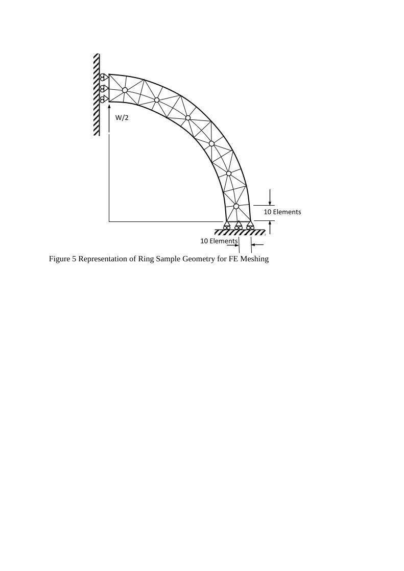
Figure 5 Representation of Ring Sample Geometry for FE Meshing

10 Elements

10 Elements

W/2

Figure 6 Measured and predicted variations in ring stiffness with sample size, 1/t2, for high aspect ratio, R/t = 8.0, rings containing three different void sizes

Figure 7 Measured and predicted variations in ring stiffness with sample size, 1/t2, for low aspect ratio, R/t = 4.0, rings containing three different void sizes

Figure 8 Load Displacement Response for Smallest Low Aspect Ratio Sample Containing 2.381 mm Diameter Voids

Figure 9 Predicted variations in low aspect ratio, R/t = 4.0, ring stiffness with sample size, 1/t2, for coupling numbers, N, values of 0.0 and 0.99

Figure 10 RMS error in predicted stiffness of all low aspect ratio, R/t = 4.0, samples with 1.588 mm voids as a function of coupling number

Figure 11 Predicted variations in low aspect ratio, R/t = 4.0, ring stiffness with sample size, 1/t2, for coupling numbers, N, values of 0.0, 0.99 and 0.175

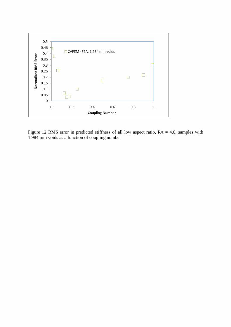
Figure 12 RMS error in predicted stiffness of all low aspect ratio, R/t = 4.0, samples with 1.984 mm voids as a function of coupling number

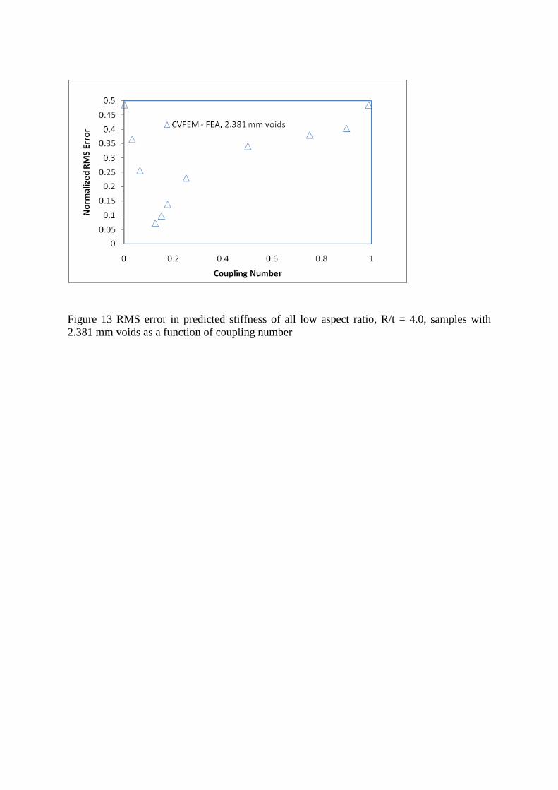
Figure 13 RMS error in predicted stiffness of all low aspect ratio, R/t = 4.0, samples with 2.381 mm voids as a function of coupling number