www.developersdilemma.org

Researching structural change & inclusive growth

Author(s): Cinar Baymul1 and Kunal Sen2

Affiliation(s): 1,2Global Development Institute, University of Manchester

Date: 18 May 2018

Email(s): kunal.sen@manchester.ac.uk

ESRC GPID Research Network Working Paper 10

Was Kuznets Right? New Evidence on the Relationship

between Structural Transformation and Inequality

WAS KUZNETS RIGHT?

2

ABSTRACT

We examine the Kuznets postulate that structural transformation leads to higher inequality

using comparable panel data for a large number of developing and developed countries for

1960-2012. Countries show different paths of structural transformation, being either

structurally under-developed, structurally developing or structurally developed. In contrast to

the Kuznets hypothesis, we find that the movement of workers to manufacturing

unambiguously decreases income inequality, irrespective of the stage of structural

transformation that a particular country is in. We also find that while the movement of

workers into services has no discernible overall impact on inequality across our set of

countries, structural transformation relating to services increases inequality in structural

developing countries and decreases inequality in structurally developed countries. Overall,

our findings confirm the positive development effects that structural transformation relating

to manufacturing may have in developing countries, not merely through higher growth but by

reducing inequality as well. However, for the vast majority of low income countries, where

manufacturing driven structural transformation seems a remote possibility, our findings

suggest that inequality will increase with the movement of workers from agriculture to

services.

KEYWORDS

structural transformation, inequality, Kuznets, manufacturing, services

WAS KUZNETS RIGHT?

3

About the GPID research network:

The ESRC Global Poverty and Inequality Dynamics (GPID) research network is an international network of academics, civil society organisations, and policymakers. It was launched in 2017 and is funded by the ESRC’s Global Challenges Research Fund. The objective of the ESRC GPID Research Network is to build a new research programme that focuses on the relationship between structural change and inclusive growth. See: www.gpidnetwork.org

THE DEVELOPER’S DILEMMA

The ESRC Global Poverty and Inequality Dynamics (GPID) research network is concerned with what we have called ‘the developer’s dilemma’.

This dilemma is a trade-off between two objectives that developing countries are pursuing. Specifically:

1. Economic development via structural transformation and productivity growth based on the intra- and inter-sectoral reallocation of economic activity.

2. Inclusive growth which is typically defined as broad-based economic growth benefiting the poorer in society in particular.

Structural transformation, the former has been thought to push up inequality. Whereas the latter, inclusive growth implies a need for steady or even falling inequality to spread the benefits of growth widely. The ‘developer’s dilemma’ is thus a distribution tension at the heart of economic development.

WAS KUZNETS RIGHT?

4

1. Introduction

Structural transformation – the movement of workers from low productivity to high productivity

activities and sectors – is an essential feature of rapid and sustained growth. The speed at which

structural transformation occurs differentiates successful countries from unsuccessful ones (Kuznets

and Murphy 1966). At the same time, since Kuznets’ seminal (1955) piece, it is widely believed that

structural transformation can lead to higher inequality, at least initially. Therefore, rapid structural

transformation may entail a trade-off between growth and inequality, which may be called the

developer’s dilemma (Sumner 2017). As Kuznets argued, while inequality may increase at the early

stages of structural transformation, beyond a certain level of structural transformation, inequality will

decrease, giving rise to the famous inverted U-shaped relationship between income and inequality – the

so-called Kuznets curve.

Several recent papers have looked at the relationship between structural transformation and economic

growth (Duarte and Restuccia 2010, Dabla-Norris et al. 2013, Herrendorf et al. 2014, McMillan et al.

2014, Diao et al. 2017, Haraguchi et al. 2017).1 In this paper, we examine the inequality dimension of

structural transformation. We re-examine the Kuznets postulate that at the early process of structural

transformation, inequality increases as workers move from a sector with low average incomes and lower

within-sector inequality – agriculture – to a sector with higher average income and higher within-sector

inequality, such as manufacturing. We argue that both from conceptual and empirical standpoints, there

are reasons to question the Kuznets view on the relationship between structural transformation and

inequality. Firstly, from a conceptual point of view, a closer examination of the assumptions behind the

Kuznets process makes clear that it is not obvious that a movement of workers from agriculture to

manufacturing necessarily involves an increase in inequality. In contrast, the movement of workers from

agriculture to services may have a different implication for inequality, as the assumptions that underlie

the Kuznets argument on the positive effect of structural transformation on inequality is more likely to

be true for the services driven structural transformation.

1 A separate (and large) literature has looked at the validity of the so-called Kuznets curve- the inverted U shaped relationship between inequality and the level of per capita income – without finding an unambiguous support for the Kuznets curve hypothesis of inequality first increasing and then decreasing with economic development (Anand and Kanbur 1993a, 1993b, Milanović 2000, Lindert and Williamson 2003, Roine and Waldenström 2015). However, this literature has focused on the growth-inequality relationship, while our interest in this paper is in the structural transformation-inequality relationship. One paper that looks at the effect of structural transformation on inequality is Angeles (2009). However, this paper does not differentiate between manufacturing and services driven structural transformation (by using total non-agricultural employment share as the core explanatory variable), which as we will show in this paper, have very different effects on inequality.

WAS KUZNETS RIGHT?

5

Secondly, as we will document later in this paper, in contrast to what was envisaged by Kuznets, for

many developing countries, the movement of workers from agriculture even in the early stage of

structural transformation has been primarily to services and not to manufacturing. Given that few

countries outside of East Asia have seen a typical path of structural transformation that was witnessed

originally among the advanced market economies where workers first moved from agriculture to

manufacturing and then on to services, it is not clear whether the implications of structural

transformation for increasing inequality may be the same for the many different paths of structural

transformation that we observe in the developing and developed world.

Our historical data from 1960 to 2012 shows three different paths or stages of structural transformation.

Firstly, there are a set of countries where the proportion of workers in agriculture is higher than any

other sector for the most recent period for which we have the data– we call this set of countries

structurally under-developed. These are mostly low-income countries. Secondly, for a set of countries,

mostly in the middle-income category, the proportion of workers in services is higher than that in

agriculture, though the share of workers in agriculture still higher than that in manufacturing. We call

this set of countries structurally developing. Finally, we have a set of countries, which are a mix of

middle and high-income countries, where the share of workers in manufacturing is higher than that in

agriculture. We call this set of countries structurally developed.

In this paper, we examine the inequality implications of structural transformation for a range of low,

middle and high-income countries from 1960 to 2012, allowing for the heterogeneity of the paths of

structural transformation that we observe in the data. We also allow for the possibility that

manufacturing driven structural transformation may have very different implications for inequality than

services driven inequality. To examine the structural transformation-inequality relationship, we use two

high quality data-sets which have become recently available, one for structural transformation and the

other for income inequality. The data for structural transformation – that is, the share of workers in

agriculture, manufacturing and services – comes from the Groningen Growth and Development Centre

(GGDC) data-base,2 which provides consistent annual data on sectoral employment for several countries

from the 1950s onwards and the data for inequality comes from the most recent revisions to the World

Income Inequality Data-base (WIID) which provides comparable inequality data over time for a large

number of countries.3

Using the GGDC and WIID data-bases and panel data methods, we find that the Kuznets postulate does

not hold true for manufacturing driven structural transformation. No matter at what stage of structural

transformation a county may be in, manufacturing unambiguously decreases inequality – the marginal

effect of an increase in manufacturing employment share on income inequality (as measured by the

2 See https://www.rug.nl/ggdc/productivity/10-sector/. 3 See https://www.wider.unu.edu/project/wiid-world-income-inequality-database.

WAS KUZNETS RIGHT?

6

Gini) is always negative and statistically significant, at all levels of manufacturing employment share.

In contrast, we find that the marginal effect of an increase in the share of workers in services is positive

on inequality for structurally developing countries, and negative for structurally developed countries, a

process which is more in line with the original Kuznets argument. Given that the bulk of the movement

of workers from agriculture are going to services and not to manufacturing in many low-income

countries, this suggests that the Kuznets argument holds with greater force in contemporary times, but

not in the manner envisaged by Kuznets and other scholars.

The rest of the paper is in six sections. In the next section, we discuss the argument proposed by Kuznets

on the relationship between structural transformation and inequality, known in the literature as the

Kuznets process. In Section 3, we describe the patterns of structural transformation in our sample of

countries. In Section 4, we provide descriptive evidence on the relationship between structural

transformation and inequality. In Section 5, we discuss the econometric methodology. We present our

results in Section 6. Section 7 concludes.

2. The Kuznets Process

In his classic 1955 paper, Kuznets suggested that in the early phase of economic development, inequality

will increase. At a later phase of economic development, as governments follow redistributive policies

combining progressive taxation with welfare spending, inequality may decrease. The core of Kuznet’s

argument on the relationship between inequality and development is captured in the following paragraph

extracted from his 1955 paper:

“An invariable accompaniment of growth in developed countries is the shift away from

agriculture, a process usually referred to as industrialization and urbanization. The income

distribution of total population in the simplest model, may therefore be viewed as a combination

of the total income distributions of the rural and urban populations. What little we know of the

structure of the two component income distributions reveals that a) the average per capita

income of the rural population is usually lower than that of the urban; b) inequality in the

percentage shares within the distribution for the rural population is somewhat narrower than

that in the urban population … Operating with this simple model, what conclusions do we

reach? First, all other conditions being unequal, the increasing weight of the urban population

means an increasing share for the more unequal of the two component distributions. Second,

the relative difference in per capita income between the rural and urban populations does not

necessarily shift downward in the process of economic growth; indeed, there is some evidence

to suggest that it is stable at best, and tends to widen because per capita productivity in urban

pursuits increases more rapidly than in agriculture. If this is so, inequality in total income

distribution should increase” (pp. 7-8).

WAS KUZNETS RIGHT?

7

The Kuznets process of widening inequality with structural transformation (that is, movement of

workers away from agriculture) can be described as composed of two sub-processes: i) between sector

inequality: a movement of the population from a sector characterised by lower mean income to a sector

characterised by higher mean income, and ii) within sector inequality: the movement of the population

from a sector with low within-sector inequality to a sector with higher within-sector inequality. If

both sub-processes work in the same direction – that is, if the movement of workers is from a sector

with both a low mean and low variance in incomes to a sector with a higher mean and high variance in

incomes, then structural transformation will unambiguously increase inequality. However, if the

movement of workers is from a sector with low mean income but higher variance of income to a sector

with a higher mean income but lower variance in income, then it is less obvious that inequality will

necessarily increase.

Following Anand and Kanbur (1993a), we provide a diagrammatic exposition of the Kuznets process

to make clear the contribution of between sector (or group) inequality and within sector (or group)

inequality to overall inequality.4 Let I be the overall measure of inequality in a given country and let x

be the share of workers in the non-agricultural sector. For the sake of exposition, let us assume that there

is only one non-agricultural sector, so that we do not make a distinction between the manufacturing and

services sectors. Let the working population of the country be normalised to one. Define between-sector

(or group) inequality as the inequality in the income distribution when a fraction x of the working

population receives income u1 and the remaining fraction, 1-x, receives income u2 (where between-

group inequality is defined as the value of the inequality measure when everyone in the sector receives

the mean income of the sector). Following Kuznets, we can assume that the mean income of the non-

agricultural sector is higher than that of the agricultural sector – that is, u1 > u2.

It is clear from between-group inequality must be zero at both x=1 and x=1, and must be positive

elsewhere – that is, when all workers are either in the agricultural sector or in the non-agricultural sector,

there can be no between-group inequality. However, in the range where x is higher than 0 but less than

1, inequality will first increase with increasing x, then fall (as captured in Figure 1). This is because

with low x, there are more workers in the low-income sector (in our example, agriculture) than in the

high-income sector, so that between sector income differences are considerable. However, once a larger

proportion of workers are in the high-income sector, between-group inequality starts falling, till it

reaches zero when all workers are in the high-income sector.

4 This exposition depends on the assumption that the inequality measures we are considering is decomposable. Among the inequality measures available in the literature, the variance of log income and mean log deviation (which is Theil’s second index) has such decomposition properties – see Robinson (1976) and Kanbur (2017).

WAS KUZNETS RIGHT?

8

Now consider the behaviour of within-group inequality. Defining within-group inequality as the

difference between overall inequality and between-group inequality, its movement with the increase in

x will depend on the assumptions that one makes on within-group inequality in the non-agricultural

sector versus the agricultural sector. If one assumes that there is higher within-group inequality in the

non-agricultural sector than in the agricultural sector (as seem to be implied by Kuznets), then the

within-group inequality component of overall inequality will strictly increase as x increases – that is,

within-group inequality will increase with structural transformation (as shown in Figure 1).

The combination of the behaviour of between-group inequality and within-group inequality may lead

to the well-known inverted relationship between structural transformation and inequality – in Figure 1,

as x increases, there is an unambiguous increase in inequality; however, once a certain x is reached, if

the between-group component dominates the within-group component, inequality will start declining.

Figure 1. The Kuznets Process

Source: adapted from Anand and Kanbur (1993a)

The Kuznets process as described above does not differentiate between whether the movement of

workers from agriculture is to manufacturing or services. Would the effects of manufacturing driven

structural transformation be different than that for services driven structural transformation? Consider

between group-inequality first. For this component to increase with structural transformation, mean

income in the sector absorbing labour from agriculture has to be higher than the mean income prevailing

in the agricultural sector. This assumption is likely to hold, no matter whether the labour absorbing

sector is manufacturing or services as productivity in the manufacturing or services sector is expected

to be higher than in agriculture, at least in the early part of industrialisation when agriculture is likely to

be characterised by surplus labour (Lewis 1954).5

5 Several studies document the much higher productivity of manufacturing and services than agriculture in low income countries (e.g., Gollin et al., 2014).

WAS KUZNETS RIGHT?

9

Now consider within-sector inequality. This component of overall inequality may not necessarily

increase with manufacturing driven structural transformation for three reasons. Firstly, the historical

experience of successful industrialisation among what are called the “late industrialisers” – for example,

China, Mauritius, South Korea, Singapore, and Taiwan – indicates that much of the early success in

industrialisation occurs in labour-intensive manufacturing, which is characterised by low within-sector

inequality (Krueger 1980, World Bank 2017). Secondly, manufacturing activity tends to be factory

based and in the formal sector (in contrast to the services sector, where a large part of economic activity

is in the informal sector), where labour markets are characterised by minimum wages and other labour

regulations. This is likely to lead to wage compression, and therefore, relatively low within-sector

inequality. Finally, there may be a political channel through which within sector inequality may decrease

with manufacturing driven structural transformation as the organised working class is likely to gain

political strength over time in countries which witness rapid industrialisation. This may lead to

democratisation that may encourage redistribution (Acemoglu and Robinson 2002).

However, a very different argument may apply to services driven structural transformation. A large of

part of the employment created in the services may be self-employment in the poorly paid informal

sector (such as household enterprises in the trade, hotels and restaurants sector), which may exist with

well-paid jobs in the formal services sector (such as banking and finance). The lack of an organised

working class in the informal services sector also does not allow workers to make demands of their

employers for better wages or of the state for redistribution. This suggests that the Kuznets argument,

which proposes that the move of workers from agriculture to non-agriculture will exacerbate the within

sector component of inequality, is likely to hold more for the services sector than the manufacturing

sector.

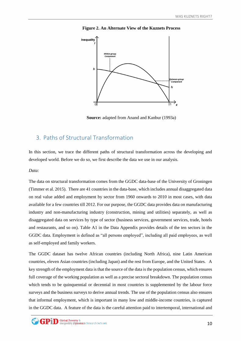
We illustrate the possibility of the within sector component of inequality falling with a movement of

workers from agriculture to manufacturing in Figure 2. Here, the within group inequality component

falls with an increase in x. As is clear from the figure, it is not obvious that inequality will necessarily

increase at early stages of structural transformation – if the within-group component of inequality

dominates the between-group component, inequality will fall with an increase in the number of workers

in the non-agricultural sector. 6

6 It should also be noted that the assumption of low within sector inequality that is being implicitly made of the agricultural sector in the Kuznets process may not be correct in many country contexts in Latin America, South Asia and Sub-Sahara Africa, where the land distribution may be concentrated among a few land-owning elites.

WAS KUZNETS RIGHT?

10

Figure 2. An Alternate View of the Kuznets Process

Source: adapted from Anand and Kanbur (1993a)

3. Paths of Structural Transformation

In this section, we trace the different paths of structural transformation across the developing and

developed world. Before we do so, we first describe the data we use in our analysis.

Data:

The data on structural transformation comes from the GGDC data-base of the University of Groningen

(Timmer et al. 2015). There are 41 countries in the data-base, which includes annual disaggregated data

on real value added and employment by sector from 1960 onwards to 2010 in most cases, with data

available for a few countries till 2012. For our purpose, the GGDC data provides data on manufacturing

industry and non-manufacturing industry (construction, mining and utilities) separately, as well as

disaggregated data on services by type of sector (business services, government services, trade, hotels

and restaurants, and so on). Table A1 in the Data Appendix provides details of the ten sectors in the

GGDC data. Employment is defined as “all persons employed”, including all paid employees, as well

as self-employed and family workers.

The GGDC dataset has twelve African countries (including North Africa), nine Latin American

countries, eleven Asian countries (including Japan) and the rest from Europe, and the United States. A

key strength of the employment data is that the source of the data is the population census, which ensures

full coverage of the working population as well as a precise sectoral breakdown. The population census

which tends to be quinquennial or decennial in most countries is supplemented by the labour force

surveys and the business surveys to derive annual trends. The use of the population census also ensures

that informal employment, which is important in many low and middle-income countries, is captured

in the GGDC data. A feature of the data is the careful attention paid to intertemporal, international and

WAS KUZNETS RIGHT?

11

internal consistency (Timmer and Vries 2009, Diao et al. 2017). This differentiates the quality of the

data from other sources of employment data, such as the International Labour Organisation’s ILOSTAT,

which compiles data directly obtained from country sources without the consistency checks undertaken

by GGDC.7 We provide further discussion on the suitability of alternate sources of sectoral employment

data for our analysis in Appendix A2.

The GGDC data has two limitations – firstly, it has limited coverage of low income countries, and

secondly, ten countries do not report disaggregated employment data for community, social and

personal services and government services. 8 According to the GGDC data, Government services

employ 13 % of the working population in average with maximum rising up to 35 % (Sweden in 1993).

The average employment rate in personal services is 6%, with the maximum being 17 % (Hong Kong

in 1981). Employment rate in these subsectors also vary over time, as we will later demonstrate in Table

3. Since both sub-sectors employ a large portion of the population, we are unable to include countries

with missing data in our own sample, as calculating averages would significantly inflate actual

employment rates in other sectors. Hence, our sample size reduces to 31 countries. We address the

limitation of a small sample size in the econometric analysis that we undertake by using the ILOSTAT

data which includes several more low-income countries as a robustness check and including imputations

of employment in community, social and personal services and government services where the data is

missing for specific country-years as an additional robustness check.

We categorise our countries by the different stage of structural transformation that they are in. A first

set of countries are those where agriculture is still the largest sector in terms of the share of employment

in the most recent time period available. In our sample, these countries are Ethiopia, India, Kenya,

Malawi, Nigeria, Senegal, and Tanzania. These countries are all in Sub-Saharan Africa, with only India

being the non-African country. We call these countries structurally under-developed. The next set of

countries are where more people are employed in the services sector than agriculture, with agriculture

being the second largest sector. These countries are Botswana, Brazil, People’s Republic of China, Costa

Rica, Ghana, Indonesia, Philippines, Thailand and South Africa. We call them structurally developing

countries. These countries span all three continents – Africa, Asia and Latin America. The final set of

countries has more people employed in manufacturing sector than agriculture. These countries in the

sample are Argentina, Hong Kong (China), Malaysia, Mauritius, Mexico, and Taiwan, as well as

Denmark, France, Italy, Japan, Netherlands, Spain, Sweden, United Kingdom and United States. These

7 As discussed in Appendix A2, an alternate source of employment data is the labour force surveys (as in the International Labour Organisation’s ILOSTAT). Though labour force surveys are more frequent than the population census, the data is often not representative in many developing countries and are sometimes restricted to particular regional areas, such as urban areas. 8 Bolivia, Chile, Colombia, Peru, Singapore, South Korea, Venezuela and Zambia do not have data on government services. Egypt and Morocco do not have data on personal services. In addition, Indonesia lack both only in one year, 1961.

WAS KUZNETS RIGHT?

12

countries are either in East Asia or Latin America (with the exception of Mauritius, which is in Africa),

and the advanced market economies. We call these countries structurally developed. We provide the

list of countries by stage of structural transformation in Table 1.

Figure 3. Share of Employment by Stages of Structural Transformation

Note: In percentages of total employment, unweighted averages.

Source: GGDC data, our calculations.

Table 1. Stages of Structural Transformation

Structurally Underdeveloped

(7 countries)

Structurally Developing

(9 countries)

Structurally Developed

(15 countries)

Ethiopia

India

Kenya

Malawi

Nigeria

Senegal

Tanzania

Brazil

Botswana

China

Costa Rica

Ghana

Indonesia

Philippines

Thailand

South Africa

Argentina

Denmark

France

Hong Kong

Italy

Japan

Malaysia

Mauritius

Mexico

Netherlands

Spain

Sweden

Taiwan

United Kingdom

United States

Note: Structurally underdeveloped: share of employment in agriculture higher than in manufacturing or

services; structurally developing: share of employment in services higher than in agriculture; structurally

developed: share of employment in manufacturing higher than in agriculture.

0.00

10.00

20.00

30.00

40.00

50.00

60.00

70.00

80.00

90.00

100.00

Under-developed Developing Developed

Agriculture Manufacturing Industry Non-manufacturing Industry Services

WAS KUZNETS RIGHT?

13

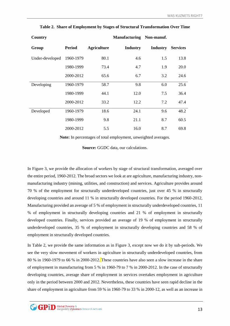
Table 2. Share of Employment by Stages of Structural Transformation Over Time

Country

Group Period Agriculture

Manufacturing

Industry

Non-manuf.

Industry Services

Under-developed 1960-1979 80.1 4.6 1.5 13.8

1980-1999 73.4 4.7 1.9 20.0

2000-2012 65.6 6.7 3.2 24.6

Developing 1960-1979 58.7 9.8 6.0 25.6

1980-1999 44.1 12.0 7.5 36.4

2000-2012 33.2 12.2 7.2 47.4

Developed 1960-1979 18.6 24.1 9.6 48.2

1980-1999 9.8 21.1 8.7 60.5

2000-2012 5.5 16.0 8.7 69.8

Note: In percentages of total employment, unweighted averages.

Source: GGDC data, our calculations.

In Figure 3, we provide the allocation of workers by stage of structural transformation, averaged over

the entire period, 1960-2012. The broad sectors we look at are agriculture, manufacturing industry, non-

manufacturing industry (mining, utilities, and construction) and services. Agriculture provides around

70 % of the employment for structurally underdeveloped countries, just over 45 % in structurally

developing countries and around 11 % in structurally developed countries. For the period 1960-2012,

Manufacturing provided an average of 5 % of employment in structurally underdeveloped countries, 11

% of employment in structurally developing countries and 21 % of employment in structurally

developed countries. Finally, services provided an average of 19 % of employment in structurally

underdeveloped countries, 35 % of employment in structurally developing countries and 58 % of

employment in structurally developed countries.

In Table 2, we provide the same information as in Figure 3, except now we do it by sub-periods. We

see the very slow movement of workers in agriculture in structurally underdeveloped countries, from

80 % in 1960-1979 to 66 % in 2000-2012. These countries have also seen a slow increase in the share

of employment in manufacturing from 5 % in 1960-79 to 7 % in 2000-2012. In the case of structurally

developing countries, average share of employment in services overtakes employment in agriculture

only in the period between 2000 and 2012. Nevertheless, these countries have seen rapid decline in the

share of employment in agriculture from 59 % in 1960-79 to 33 % in 2000-12, as well as an increase in

WAS KUZNETS RIGHT?

14

the share of employment in manufacturing from 10 % in 1970-79 to 12 % in 2000-12. For structurally

developed, the share of employment in agriculture was low to start with at 19 % in 1970-79. By the time

we reach the period 2000-12, more workers are employed in non-manufacturing industry in these

countries than in agriculture, and services at 70 % provide the largest employment by far. Here, we

observe a fall in the share of employment in manufacturing over time.

Figure 4. Share of Employment in Services Sub-Sectors by Country Group – Period Average

Note: In percentages of total employment, unweighted averages.

Source: GGDC data, our calculations.

Table 3. Share of Employment in Services Sub-Sectors by Country Group Over Time

Country

Group Period Services Business

Transpor

t Trade Govt. Personal

Under-

developed 1960-1979

13.8

0.3 1.4 5.8 3.6 2.8

1980-1999 20.0 0.5 1.7 9.4 4.5 3.8

2000-2012 24.6 0.9 2.3 12.4 4.9 4.0

Developing 1960-1979 25.6 1.9 2.7 9.4 6.8 4.9

1980-1999 36.4 3.1 3.4 13.4 9.8 6.6

2000-2012 47.4 5.1 4.6 19.3 10.7 7.6

Developed 1960-1979 48.2 4.5 6.2 16.3 15.9 5.3

1980-1999 60.5 7.9 6.5 19.5 19.8 6.7

2000-2012 69.8 12.2 6.7 21.7 21.7 7.7

Note: In percentages of total employment, unweighted averages.

Source: GGDC data, our calculations.

0.00

10.00

20.00

30.00

40.00

50.00

60.00

70.00

Under-developed Developing DevelopedBusiness Transport Trade Government Personal

WAS KUZNETS RIGHT?

15

The share of employment in the five sub-sectors that make up the total services sector, business,

transport, trade, government and personal services, also differ between country groups as well over

time. While the trade sub-sector which includes wholesale and retail trade, as well as restaurants and

hotels, is the largest sub-sector within services in both under-developed and developing countries in our

sample in almost all the periods, government services catch up to the trade sub-sector in structurally

developed countries over the past three decades (Figure 4). Apart from the government services sub-

sector, the most rapid increase for a particular sub-sector within the services sector is observed in the

business services sub-sector for the structurally developing and developed countries – in the former

group of countries, it goes up from 1.9 % of total employment in 1960-79 to 5.7 % in 2000-12, and for

the latter group of countries, for the same periods, it goes up from 4.5 % to 12.2 % (Table 3). In contrast,

the business services sub-sector remains a paltry 0.9 % of total employment in structurally

underdeveloped countries in 2000-12.

Figures 5-8. Movement of Workers from Agriculture to Manufacturing and Services over Time

Figure 5. All Countries Figure 6. Structurally Underdeveloped

Countries

Figure 7. Structurally Developing Countries Figure 8 . Structurally Developed Countries

Note: Manufacturing-Agriculture: Employment Share in Manufacturing – Employment Share in Agriculture,

Manufacturing-Services: Employment Share in Services – Employment Share in Agriculture; unweighted

averages.

Source: GGDC data, our calculations.

WAS KUZNETS RIGHT?

16

A striking feature of structural transformation in our 31 countries is that the movement of employment

from agriculture has been mostly to services (Figure 5). For structurally underdeveloped countries,

there was a sharp incline in the movement of workers away from agriculture till the mid-1970s, then a

reduction since then (Figure 6). We observe a rapid and sustained movement of workers from

agriculture to manufacturing and services in structurally developing countries over the entire period

1960-2012, which is very different to what we observed in structurally underdeveloped countries

(Figure 7). Finally, for structurally developed countries, the movement of workers from agriculture is

mostly to services, with the movement of workers from agriculture to manufacturing falling over time

(Figure 8).

Figures 9-12. Relative Productivity Differentials over Time

Figure 9. All Countries Figure 10. Structurally Underdeveloped

Countries

Figure 11. Structurally Developing Countries Figure 12. Structurally Developed Countries

Note: Manufacturing Prod./Agri Prod.: Real Value Added per Worker in Manufacturing as Ratio of Real Value

Added per Worker in Agriculture; Services Prod./Agri Prod.: Real Value Added per Worker in Services as

Ratio of Real Value Added per Worker in Agriculture; unweighted averages.

Source: GGDC data, our calculations.

WAS KUZNETS RIGHT?

17

A second striking feature of structural transformation has been that the shift of employment from

agriculture to services has been accompanied by falling relative productivity of services to agriculture

(Figure 9).9 In contrast, the relative productivity of manufacturing to agriculture has increased till the

1970s, then showed a sharp decline until 1980s, and is significantly higher than the relative productivity

of the services sector since mid-1980s. This suggests that a services driven structural transformation has

very different implications for overall productivity growth as compared to a manufacturing driven

structural transformation (Herrendorf et al. 2014).10 We also observe very different patterns of relative

productivity movements over time across the three different country groups – consistent with the slow

movement of workers from agriculture to manufacturing, manufacturing relative productivity levels are

very similar to that of services in structurally underdeveloped countries (Figure 10). In contrast, for

structurally developing countries, which have seen an increasing share of manufacturing employment

in total employment, the relative productivity of manufacturing is significantly higher than that of

services (Figure 11). For structurally developed countries, where agricultural productivity levels are

high relative to what we observe in structurally underdeveloped and developing countries (see Gollin et

al. 2014), relative productivity differences across sectors become insignificant over time as more

workers move out of agriculture (Figure 12).

Figure 13. Structural Transformation and Within Sector Inequality in Manufacturing

Source: https://utip.lbj.utexas.edu/data.html, our calculations.

9 We measure sectoral productivity as the ratio of real value added to total employment in the sector. The data is obtained from the GGDC data-base. 10 This observation is also supported by the cross-country analysis undertaken by Duarte and Restuccia (2010) who show that productivity catch-up in industry explain about 50 per cent of the gains in aggregate productivity across countries, whereas low productivity in services and the lack of catch-up explain economic stagnation in low income countries.

WAS KUZNETS RIGHT?

18

In the previous section, we argued that one key assumption behind the Kuznets process – that the within-

sector component of total inequality will increase at the early stages of structural transformation - may

not necessarily hold if the movement of workers from agriculture is to manufacturing. We now provide

some suggestive evidence to support our claim that manufacturing in the early stages of structural

transformation may not be characterised by high within-sector inequality. To capture within-sector

inequality manufacturing, we use the Theil measure of within industry pay inequality as calculated by

the University of Texas Inequality Project (UTIP) using industry-specific wage data from the United

Nations Industrial Development Organisation (UNIDO)’s industrial statistics data-base (see Galbraith

et al. 2014). We present the relationship between manufacturing employment share and the Theil

measure of within industry pay inequality by our country groups in Figure 13. We observe that for the

set of countries which are at the relatively early stages of industrialisation – the structurally

underdeveloped and developing countries – within sector inequality in manufacturing decreases with

increases in the manufacturing employment share (this is not the case for the structurally developed

countries). Particularly for countries where the share of employment in manufacturing has been very

high (at over 20 %) in certain periods such as Hong Kong, Malaysia, Mauritius and Taiwan, the

decreases in within sector inequality can be explained by the fact that much of the increase in

employment occurred in the labour-intensive manufacturing sectors (Krueger 1978, Riedel 1988)

What about within sector inequality in services? We do not have data on mean incomes by sub-sector

in services to allow us to compute within sector inequality in services. However, using productivity as

a proxy for mean incomes at the sub-sectoral level, we find clear differences in relative productivity

levels across sub-sectors – the Business Services sub-sector which comprise finance, banking and

information technology, is far more productive than all other Services sub-sectors (Figure 14), and we

see that this productivity gap has widened over time. This suggests that there is widening within-sector

inequality in services as the business services sub-sector grew in importance, particularly in structurally

developing and developed countries (as we noted earlier in this section).

WAS KUZNETS RIGHT?

19

Figure 14. Relative Productivity within Services sector over time, All Countries

Note: Trade P./AP: Real Value Added per Worker in Trade Services as Ratio of Real Value Added per Worker in

Agriculture; Transport P./AP: Real Value Added per Worker in Transport Services as Ratio of Real Value Added

per Worker in Agriculture; Business P./AP: Real Value Added per Worker in Business Services as Ratio of Real

Value Added per Worker in Agriculture; Govt P./AP: Real Value Added per Worker in Government Services as

Ratio of Real Value Added per Worker in Agriculture; Pers. P./AP: Real Value Added per Worker in Personal,

Social and Community Services as Ratio of Real Value Added per Worker in Agriculture; unweighted averages.

Source: GGDC data, our calculations.

Overall, our analysis of the patterns of structural transformation suggests that different countries in

Africa, Asia, Europe and North America and Latin America have shown very different paths of

structural transformation over time, both in the across-sector movement of workers as well as the

behaviour of relative productivities over time at the sectoral level. We next discuss the implications of

these different paths of structural transformation for inequality.

4. Patterns of Structural Transformation and Inequality

Data for income inequality are taken from the standardized income inequality dataset, prepared by

Baymul and Shorrocks (2018), which is a revision of the WIID data-base of the World Institute for

Development Economics Research. The Gini coefficient is the most commonly used measure of

inequality; however, conceptual and methodological differences between household surveys that are

used to calculate Gini coefficients make their comparability between countries and over time

problematic. The standardized dataset we use in this paper tries to overcome the issues of comparability

by adjusting all available data that exceeds a quality threshold from various sources through a regression

WAS KUZNETS RIGHT?

20

adjustment method that includes an extensive list of independent variables. We use Net Ginis, which

measure net per capita income inequality in a country in a given year (as a robustness test in our

econometric analysis, we use Gross Ginis as well).

We first look at the overall relationship between manufacturing employment share and inequality, then

by country group. In the overall sample as well as by country group, we see a clear negative relationship

between manufacturing driven structural transformation and inequality (Figures 15 and 16). In the case

of structurally developed countries, there is a suggestion that inequality increases, once manufacturing

employment share crosses 30 %; however, as Figure 15 makes clear, there are very few countries-year

observations that are over this threshold.

Figures 15-16. The Relationship between Manufacturing Employment Share and Inequality

Figure 15. All Countries Figure 16. Different Paths of Structural

Transformation

Source: GGDC data and Baymul-Shorrocks (2018), our calculations.

We next look at the relationship between services employment share and inequality, for the overall

sample and then by country group (Figures 17 and 18). We do not see a clear relationship in the overall

sample, with a lack of precision in the fitted line estimated in the scatter plot. By country group, we

seem to see a U-shaped relationship for structurally developed countries, and a positive relationship for

structurally under-developed and developing countries. Overall, the scatter plots suggest that there is a

negative relationship between manufacturing driven structural transformation and inequality and a lack

of a clear relationship between services driven structural transformation and inequality. We now proceed

to an econometric analysis of the relationship between structural transformation and inequality. We next

discuss the econometric methodology that we will use in the analysis.

WAS KUZNETS RIGHT?

21

Figures 17-18. The Relationship between Services Employment Share and Inequality

Figure 17. All Countries Figure 18. Different Paths of Structural

Transformation

Source: GGDC data and Baymul-Shorrocks (2018), our calculations.

5. Methodology

Our paper has two core research questions: a) what are the effects of manufacturing driven structural

transformation on income inequality, and do the effects differ by the path of structural transformation a

country is in, and b) what are the effects of services driven structural transformation on income

inequality, and how are they different from the effects of manufacturing driven structural

transformation? To address the first research question, we estimate the marginal impact of an increase

in the share of employment in manufacturing on inequality with the three following equations:

𝐺𝑖𝑛𝑖𝑖𝑡 = 𝛽𝑚𝑎𝑛𝑀𝑎𝑛𝑢𝑓𝑎𝑐𝑡𝑢𝑟𝑖𝑛𝑔𝑖𝑡 + 𝛽𝑚𝑖𝑛𝑀𝑖𝑛𝑖𝑛𝑔𝑖𝑡 + 𝛽𝑢𝑡𝑙𝑈𝑡𝑖𝑙𝑖𝑡𝑖𝑒𝑠𝑖𝑡

+ 𝛽𝑐𝑜𝑛𝑠𝐶𝑜𝑛𝑠𝑡𝑟𝑢𝑐𝑡𝑖𝑜𝑛𝑖𝑡 + 𝛽𝑆𝑒𝑟𝑣𝑆𝑒𝑟𝑣𝑖𝑐𝑒𝑠𝑖𝑡 + 𝛽𝑋𝑖𝑡 + 𝜎𝑡 + 𝑎𝑖 + 𝑢𝑖𝑡 (1)

𝐺𝑖𝑛𝑖𝑖𝑡 = 𝛽𝑚𝑎𝑛𝑀𝑎𝑛𝑢𝑓𝑎𝑐𝑡𝑢𝑟𝑖𝑛𝑔𝑖𝑡 + 𝛽𝑚𝑎𝑛𝑠𝑞𝑀𝑎𝑛𝑢𝑓𝑎𝑐𝑡𝑢𝑟𝑖𝑛𝑔𝑖𝑡2 + 𝛽𝑚𝑖𝑛𝑀𝑖𝑛𝑖𝑛𝑔𝑖𝑡

+ 𝛽𝑢𝑡𝑙𝑈𝑡𝑖𝑙𝑖𝑡𝑖𝑒𝑠𝑖𝑡 + 𝛽𝑐𝑜𝑛𝑠𝐶𝑜𝑛𝑠𝑡𝑟𝑢𝑐𝑡𝑖𝑜𝑛𝑖𝑡 + 𝛽𝑆𝑒𝑟𝑣𝑆𝑒𝑟𝑣𝑖𝑐𝑒𝑠𝑖𝑡 + 𝛽𝑋𝑖𝑡 + 𝜎𝑡

+ 𝑎𝑖 + 𝑢𝑖𝑡

(2)

𝐺𝑖𝑛𝑖𝑖𝑡 = 𝛽𝑚𝑎𝑛𝑀𝑎𝑛𝑢𝑓𝑎𝑐𝑡𝑢𝑟𝑖𝑛𝑔𝑖𝑡 + 𝛽𝑚𝑖𝑛𝑀𝑖𝑛𝑖𝑛𝑔𝑖𝑡 + 𝛽𝑢𝑡𝑙𝑈𝑡𝑖𝑙𝑖𝑡𝑖𝑒𝑠𝑖𝑡

+ 𝛽𝑐𝑜𝑛𝑠𝐶𝑜𝑛𝑠𝑡𝑟𝑢𝑐𝑡𝑖𝑜𝑛𝑖𝑡 + 𝛽𝑆𝑒𝑟𝑣𝑆𝑒𝑟𝑣𝑖𝑐𝑒𝑠𝑖𝑡 + 𝛽𝐷𝑒𝑣𝑒𝑙𝑜𝑝𝑒𝑑𝑖

+ 𝛽𝐷𝑒𝑣𝑒𝑙𝑜𝑝𝑖𝑛𝑔𝑖 + 𝛽𝐷𝑒𝑣𝑒𝑙𝑜𝑝𝑒𝑑 ∗ 𝑀𝑎𝑛𝑢𝑓𝑎𝑐𝑡𝑢𝑟𝑖𝑛𝑔𝑖𝑡

+ 𝛽𝐷𝑒𝑣𝑒𝑙𝑜𝑝𝑖𝑛𝑔 ∗ 𝑀𝑎𝑛𝑢𝑓𝑎𝑐𝑡𝑢𝑟𝑖𝑛𝑔𝑖𝑡 + 𝛽𝑋𝑖𝑡+𝜎𝑡 + 𝑎𝑖 + 𝑢𝑖𝑡

(3)

WAS KUZNETS RIGHT?

22

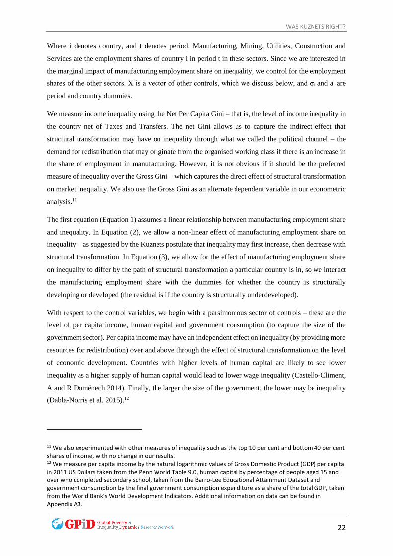
Where i denotes country, and t denotes period. Manufacturing, Mining, Utilities, Construction and

Services are the employment shares of country i in period t in these sectors. Since we are interested in

the marginal impact of manufacturing employment share on inequality, we control for the employment

shares of the other sectors. X is a vector of other controls, which we discuss below, and σt and ai are

period and country dummies.

We measure income inequality using the Net Per Capita Gini – that is, the level of income inequality in

the country net of Taxes and Transfers. The net Gini allows us to capture the indirect effect that

structural transformation may have on inequality through what we called the political channel – the

demand for redistribution that may originate from the organised working class if there is an increase in

the share of employment in manufacturing. However, it is not obvious if it should be the preferred

measure of inequality over the Gross Gini – which captures the direct effect of structural transformation

on market inequality. We also use the Gross Gini as an alternate dependent variable in our econometric

analysis.11

The first equation (Equation 1) assumes a linear relationship between manufacturing employment share

and inequality. In Equation (2), we allow a non-linear effect of manufacturing employment share on

inequality – as suggested by the Kuznets postulate that inequality may first increase, then decrease with

structural transformation. In Equation (3), we allow for the effect of manufacturing employment share

on inequality to differ by the path of structural transformation a particular country is in, so we interact

the manufacturing employment share with the dummies for whether the country is structurally

developing or developed (the residual is if the country is structurally underdeveloped).

With respect to the control variables, we begin with a parsimonious sector of controls – these are the

level of per capita income, human capital and government consumption (to capture the size of the

government sector). Per capita income may have an independent effect on inequality (by providing more

resources for redistribution) over and above through the effect of structural transformation on the level

of economic development. Countries with higher levels of human capital are likely to see lower

inequality as a higher supply of human capital would lead to lower wage inequality (Castello-Climent,

A and R Doménech 2014). Finally, the larger the size of the government, the lower may be inequality

(Dabla-Norris et al. 2015).12

11 We also experimented with other measures of inequality such as the top 10 per cent and bottom 40 per cent shares of income, with no change in our results. 12 We measure per capita income by the natural logarithmic values of Gross Domestic Product (GDP) per capita in 2011 US Dollars taken from the Penn World Table 9.0, human capital by percentage of people aged 15 and over who completed secondary school, taken from the Barro-Lee Educational Attainment Dataset and government consumption by the final government consumption expenditure as a share of the total GDP, taken from the World Bank’s World Development Indicators. Additional information on data can be found in Appendix A3.

WAS KUZNETS RIGHT?

23

We estimate Equations 1 and 2 by panel fixed effects regressions to control for time-invariant country

characteristics (such as the country’s factor endowments) that may explain both the pattern of structural

transformation and inequality.13 We estimate the third equation by random effects as it contains time

invariant dummy variables for structurally developing and developed countries that need to be

estimated. We also include period dummies to control for common global shocks that may affect

structural transformation and inequality.14

To address the second research question, we estimate the following two equations to examine whether

a relationship exists between income inequality and services driven structural transformation using fixed

effects regressions for Equation (4) and random effects regressions for Equation (5):

𝐺𝑖𝑛𝑖𝑖𝑡 = 𝛽𝑠𝑒𝑟𝑣𝑆𝑒𝑟𝑣𝑖𝑐𝑒𝑠𝑖𝑡 + 𝛽𝑠𝑒𝑟𝑣𝑠𝑞𝑆𝑒𝑟𝑣𝑖𝑐𝑒𝑠𝑖𝑡2 + 𝛽𝑚𝑖𝑛𝑀𝑖𝑛𝑖𝑛𝑔𝑖𝑡 + 𝛽𝑢𝑡𝑙𝑈𝑡𝑖𝑙𝑖𝑡𝑖𝑒𝑠𝑖𝑡

+ 𝛽𝑐𝑜𝑛𝑠𝐶𝑜𝑛𝑠𝑡𝑟𝑢𝑐𝑡𝑖𝑜𝑛𝑖𝑡 + 𝛽𝑚𝑎𝑛𝑀𝑎𝑛𝑢𝑓𝑎𝑐𝑡𝑢𝑟𝑖𝑛𝑔𝑖𝑡 + 𝛽𝑋𝑖𝑡 + 𝑎𝑖 + 𝑢𝑖𝑡 (4)

𝐺𝑖𝑛𝑖𝑖𝑡 = 𝛽𝑆𝑒𝑟𝑣𝑆𝑒𝑟𝑣𝑖𝑐𝑒𝑠𝑖𝑡 + 𝛽𝑚𝑖𝑛𝑀𝑖𝑛𝑖𝑛𝑔𝑖𝑡 + 𝛽𝑢𝑡𝑙𝑈𝑡𝑖𝑙𝑖𝑡𝑖𝑒𝑠𝑖𝑡 + 𝛽𝑐𝑜𝑛𝑠𝐶𝑜𝑛𝑠𝑡𝑟𝑢𝑐𝑡𝑖𝑜𝑛𝑖𝑡

+ 𝛽𝑚𝑎𝑛𝑀𝑎𝑛𝑢𝑓𝑎𝑐𝑡𝑢𝑟𝑖𝑛𝑔𝑖𝑡 + 𝛽𝐷𝑒𝑣𝑒𝑙𝑜𝑝𝑒𝑑𝑖 + 𝛽𝐷𝑒𝑣𝑒𝑙𝑜𝑝𝑖𝑛𝑔𝑖

+ 𝛽𝐷𝑒𝑣𝑒𝑙𝑜𝑝𝑒𝑑 ∗ 𝑆𝑒𝑟𝑣𝑖𝑐𝑒𝑠𝑖𝑡 + 𝛽𝐷𝑒𝑣𝑒𝑙𝑜𝑝𝑖𝑛𝑔 ∗ 𝑆𝑒𝑟𝑣𝑖𝑐𝑒𝑠𝑖𝑡 + 𝛽𝑋𝑖𝑡 + 𝑎𝑖

+ 𝑢𝑖𝑡

(5)

As we noted earlier, we have missing data for several years at the sub-sectoral level for the community,

social and personal services and government services for 10 countries (see Footnote 8). This implies

that for these countries, the share of employment in manufacturing and services is measured with error

as we do not know what the true level of employment in these countries for the years when the data on

sub-sectoral services is missing. Further, data on the Gini coefficient is not available on an annual basis,

with usually one observation for a five-year period for many countries. In addition, data on one of our

control variables - human capital – is unavailable for Ethiopia and Nigeria. We begin our econometric

analysis with the 29 countries for which we have complete data on the core explanatory variables – the

manufacturing and services employment shares – as well as all our basic set of control variables. We

use five-year averaged data to take into account the infrequent nature of the data on income inequality.

We have 219 observations for the 29 countries for the period 1960-2012. This is our basic empirical

specification.

13 For example, countries with more favourable endowments of unskilled labour may have both larger manufacturing sectors as well as lower inequality (see Wood 2017). 14 For example, a boom in global commodity prices may lead to a rise in employment in primary commodity sectors coinciding with an increase in inequality as incomes increase in high rent natural resource intensive activities.

WAS KUZNETS RIGHT?

24

We then proceed to do several robustness checks. Firstly, we include a further set of controls – foreign

direct investment, trade as a ratio of GDP and financial open-ness to capture the effect of globalisation

on inequality (Goldberg and Pavcnik 2007, Jaumotte et al. 2013).15 Including these set of controls

implies that we lose 30 observations – we now only have 189 observations. Secondly, we use the Gross

Gini instead of the Net Gini as our dependent variable of interest. Thirdly, we omit the rich countries in

our sample, which had largely completed their process of structural transformation prior to the

beginning year of our analysis.16 Fourthly, we impute the missing data on community, social and

personal services and government services for the countries where the data is missing.17 Finally, we use

data from ILOSTAT, where we have many more countries in our sample (115 countries, with the total

number of observations being 475) – however, as we have noted in Section 3, the quality of the

ILOSTAT is not high, so we have a trade-off between quality of the data and quantity (that is, number

of countries and observations). We present our results in the next section.

6. Results

We present the results of the set of panel regressions that aim to investigate the relationship between the

manufacturing employment share and income inequality in Table 4 and the marginal effects of

manufacturing employment share on inequality in Table 5. 18Cols. (I) and (II) present the estimates of

equation (1) with and without our basic controls. Cols. (III) and (IV) present the estimates of equation

(2), with squared manufacturing employment share included as a regressor, with and without our basic

controls. Cols. (V) and VI) present the random effects estimates of equation (3), with country groups

interacted with manufacturing employment share.

15 Data on foreign direct investment and trade over GDP comes from World Bank’s World Development Indicators. We use the Chinn-Ito measure to capture financial open-ness, which measures the degree of capital account open-ness in the country (Chinn and Ito 2006). 16 These countries are Denmark, France, Italy, Japan, Netherland, Spain, Sweden, UK and the USA. When we drop these nine countries, we lose 87 observations. 17 We impute the missing data by first dividing the total amount of labour in each subsector to the population of the country to get the share of population working in one subsector in the total population, so as to normalize the shares across countries. Then we regressed the missing personal services share on each subsector (excluding the government services share), year dummies and country dummies. By doing so, we obtained the predicted personal shares for the missing observations. We followed the same procedure for the government services sector, but in this case, we included all subsectors since we no longer have missing personal services values. Finally, we calculated the total number of people working in personal and government services by multiplying them back with country populations. Our total number of observations increases to 294. 18 Descriptive statistics are presented in Table A2.

WAS KUZNETS RIGHT?

25

Table 4. Regression Results I

I II III IV V VI

FE I FE II FE III FE IV RE I RE II

Manufacturing -0.21***

(0.07)

-0.29***

(0.07)

-0.67*

(0.38)

-0.74**

(0.33)

-1.31**

(0.51)

-1.00**

(0.40)

Manufacturing Sq 0.01

(0.01)

0.01

(0.01)

Mining -0.80

(0.55)

-1.37**

(0.58)

-0.76

(0.58)

-1.33**

(0.60)

-0.32

(0.59)

-0.70

(0.62)

Utilities 1.54

(2.79)

2.98

(2.68)

1.62

(2.67)

3.05

(2.55)

1.01

(2.21)

2.22

(2.22)

Construction 0.55**

(0.26)

0.34

(0.22)

0.66**

(0.28)

0.46**

(0.22)

0.66**

(0.29)

0.49**

(0.24)

Services -0.14

(0.11)

-0.32**

(0.14)

--0.07

(0.15)

-0.26

(0.17)

-0.07

(0.11)

-0.20

(0.13)

lnGDP 5.97***

(1.96)

5.95***

(1.95)

4.49**

(1.90)

Secondary School

Comp.

-0.09*

(0.05)

-0.10*

(0.05)

-0.09

(0.05)

Gov Exp 0.16

(0.15)

0.16

(0.16)

0.05

(0.15)

Developed -17.12

(10.43)

-17.60*

(9.89)

Developing -5.77

(8.78)

-1.76

(7.36)

Manufacturing*

Developed

1.12**

(0.54)

0.75*

(0.43)

Manufacturing*

Developing

1.19**

(0.56)

0.61

(0.45)

No. of Obs. 219 219 219 219 219 219

R-squared (within) 0.26 0.32 0.24 0.33 0.25 0.31

F 11.64 8.79 11.12 9.89

Wald chi2 165.84 360.61

Dependent variable is Gini (Net). Standard errors in parentheses. Period dummies are included. *, **,

***: Significance in 10, 5, 1% respectively.

WAS KUZNETS RIGHT?

26

Table 5. Marginal Effect of Manufacturing Employment Share

FE IV – Marginal Effects of Manufacturing RE II – Marginal Effects of Manufacturing

Share of Manufacturing Dy/dx Country Group Dy/dx

1% -0.72** Underdeveloped -1.00**

5% -0.63** Developing -0.39*

10% -0.52*** Developed -0.25***

15% -0.41***

20% -0.30***

25% -0.19*

*, **, ***: Significance in 10, 5, 1% respectively.

The fixed effect estimates in the first and second columns (Cols. (I) and (II)) both suggest that an

increase in manufacturing employment share decreases income inequality – the coefficient on the

manufacturing employment share is negative and significant at 10 % level of significance or below. The

coefficient on Column II implies that a 1 % increase in manufacturing’s share in employment reduces

income inequality by 0.29 percentage points in the Gini index. Inclusion of the squared manufacturing

variable in Columns III and IV allows us to test whether a quadratic Kuznets-type relationship exists

between manufacturing and inequality. While the coefficient of the squared variable is insignificant, the

effect of share of manufacturing employment share on inequality remains strongly negative. The final

two columns in Table 4 display the results of the random effects regressions that aim to distinguish any

difference in the marginal impact of manufacturing on inequality between different country groups. We

find evidence of clear heterogeneity in the effects of manufacturing employment share on inequality by

country group, with the effect of manufacturing employment share on inequality being lower in

structurally developing and developed countries as compared to structurally underdeveloped countries.

We present the marginal effect of manufacturing on inequality derived from Columns (IV) and (VI) of

Table 4 in Table 5 at different levels of manufacturing employment share and by country groups. We

find that the effect of manufacturing employment share on inequality is negative and statistically

significant, irrespective of the level of manufacturing employment share. Even when manufacturing

employment share is close to the maximum of any period average between country groups (25.1 %), it

still has a negative impact on inequality. This is a remarkable finding as it suggests that manufacturing

driven structural transformation will unambiguously decrease income inequality. Similarly, we find the

effect of manufacturing employment share on inequality is negative and statistically significant for all

country groups, though the effect is the strongest for structurally underdeveloped countries.

WAS KUZNETS RIGHT?

27

With respect to the other sectoral employment variables, construction is the only one with a consistently

significant impact on inequality. Mining also has a significant and negative coefficient in fixed effects

regressions when we include all the control variables. However, the mining sector is relatively small in

most countries, so its overall effect is economically not significant. Employment share in services carries

a negative sign in all the regressions, yet it remains insignificant in all but one.

We next estimate the effects of services driven structural transformation on inequality in Table 6. Cols.

(I) and (II) present estimates of Equation (4) with and without the basic controls. Cols (III) and (IV)

present estimates of Equation (5) with and without the controls. We find that no matter whether we

include controls or not, whether we include the quadratic term for services or whether we include fixed

effects or random effects, the overall effect of services on inequality is not statistically significant (and

the sign changes from positive to negative as we move from the fixed effects to random effects

regressions).

WAS KUZNETS RIGHT?

28

Table 6. Regression Results 2

I II III IV

FE V FE VI RE III RE IV

Manufacturing -0.37**

(0.17)

-0.53**

(0.19)

-0.39***

(0.11)

-0.60***

(0.16)

Mining -0.94

(0.57)

-1.52***

(0.54)

0.06

(0.70)

0.55

(0.69)

Utilities 1.31

(2.77)

2.77

(2.71)

-0.06

(2.14)

0.39

(2.61)

Construction 0.40*

(0.24)

0.12

(0.22)

0.68**

(0.26)

0.50

(0.31)

Services 0.15

(0.39)

0.07

(0.32)

-0.34

(0.29)

-0.21

(0.32)

Services Sq -0.003

(0.005)

-0.005

(0.003)

lnGDP 6.55***

(2.05)

2.95*

(1.79)

Secondary School

Comp.

-0.08

(0.05)

-0.02

(0.05)

Gov Exp 0.12

(0.17)

-0.32**

(0.14)

Developed -2.94

(12.17)

4.95

(11.24)

Developing -13.40

(10.67)

-14.20

(10.33)

Services*

Developed

0.11

(0.29)

-0.14

(0.33)

Services*

Developing

0.54*

(0.30)

0.45

(0.34)

No. of Obs. 219 219 219 219

R-squared (within) 0.24 0.34 0.29 0.30

F 10.00 13.73

Wald chi2 153.34 218.50

Dependent variable is Gini (Net). Standard errors in parentheses. . Period dummies are included. *,

**, ***: Significance in 10, 5, 1% respectively.

WAS KUZNETS RIGHT?

29

Table 7. Marginal Effect of Services Employment Share

FE VI – Marginal Effects of Services RE II – Marginal Effects of Services

Share of Services Dy/dx Country Group Dy/dx

5% 0.02 Underdeveloped -0.21

15% -0.08 Developing 0.24*

25% -0.17 Developed -0.35***

35% -0.27*

45% -0.36**

55% -0.46***

65% -0.55***

75% -0.65**

*, **, ***: Significance in 10, 5, 1% respectively.

Table 8. Marginal Effect of Business Services Employment Share

FE VI – Marginal Effects of Business RE II – Marginal Effects of Business

Share of Business Dy/dx Country Group Dy/dx

2% -1.12*** Underdeveloped 1.18

4% -1.16*** Developing 0.59*

6% -1.21*** Developed -1.22***

8% -1.25***

10% -1.30***

12% -1.34***

14% -1.39***

16% -1.44***

18% -1.48***

*, **, ***: Significance in 10, 5, 1% respectively.

We present the marginal effect of the services employment share on inequality at different levels of

services employment share and by country group in Table 7 (using the estimates from Cols. (II) and

(IV) respectively). We find that only when the services employment share exceeds 35 %, does it start

reducing inequality. When we look at the effect of services employment share by country group, we

find that for structurally developing countries, the services employment share actually increases

inequality while decreasing inequality in structurally developed countries. For structurally

underdeveloped countries, the coefficient on services employment share is not statistically significant.

Our results suggest if the Kuznets postulate were to hold, it does not do so for manufacturing but does

so for services (where inequality increases, at least for countries where a large part of employment is in

services, then decreases for the more developed countries).

WAS KUZNETS RIGHT?

30

What may explain the surprising result we get for services driven structural transformation where it

increases inequality for structurally developing but not for structurally underdeveloped countries? We

had noted from Section III that a key growth sector in services for structurally developing countries as

compared to structurally underdeveloped countries was the business services sub-sector. We had also

noted the large productivity difference between this sub-sector and other services sub-sectors. In Table

8, we present the marginal effect of business services on inequality by level of employment in the sub-

sector and by country group. The left-side columns on the table imply that when the share of the business

sector is close to the sample average of 5 %, a further 1 % increase in its share corresponds to a decrease

in net income inequality of around 1.2 percentage points. We find that the business services

significantly increases inequality in the structurally developing countries, while decreasing it for

structurally developed countries (with no discernible effect on structurally underdeveloped countries).19

This is in accord with our intuition that the growth of the business services sub-sector leads to increases

in within-sector inequality increases in the services sector as workers in the business services sub-sector

(mostly professionals working in banking, finance and information technology) tend to be paid much

better than workers in trade, restaurants and hotels, and other services sub-sectors (where a large

proportion of employment is in the informal sector in the structurally underdeveloped and developing

countries). However, for structurally developed countries, where productivity and income differences

within services sub-sectors are not likely to be as high as in the other country groups, between sector

inequality starting dominating within-sector inequality in the overall behaviour of inequality as most

workers in the economy are now employed in the services sector (leading to the downward movement

in the between-group component of inequality, as captured in Figure 1).

Robustness Tests

We now do a battery of robustness tests to see whether our findings on the inequality decreasing effect

of manufacturing employment share and the heterogenous effect of services employment share remain

with, inclusion of additional controls, an alternate measure of inequality, and changes in our sample of

countries.

We present the marginal effects of manufacturing and services for each robustness test (full results are

available on request). First, in Table 9, we include additional controls that capture globalisation – foreign

direct investment, trade and financial open-ness. Next, we reports results when we use the Gross Gini

as our dependent variable (Table 10). Then, we report results when we exclude the advanced market

economies (Table 11). Next, we use an extended sample where we impute missing data for community,

19 We do similar analysis for the trade and transport sub-sectors but do not obtain the same findings as we do for the business services sub-sector.

WAS KUZNETS RIGHT?

31

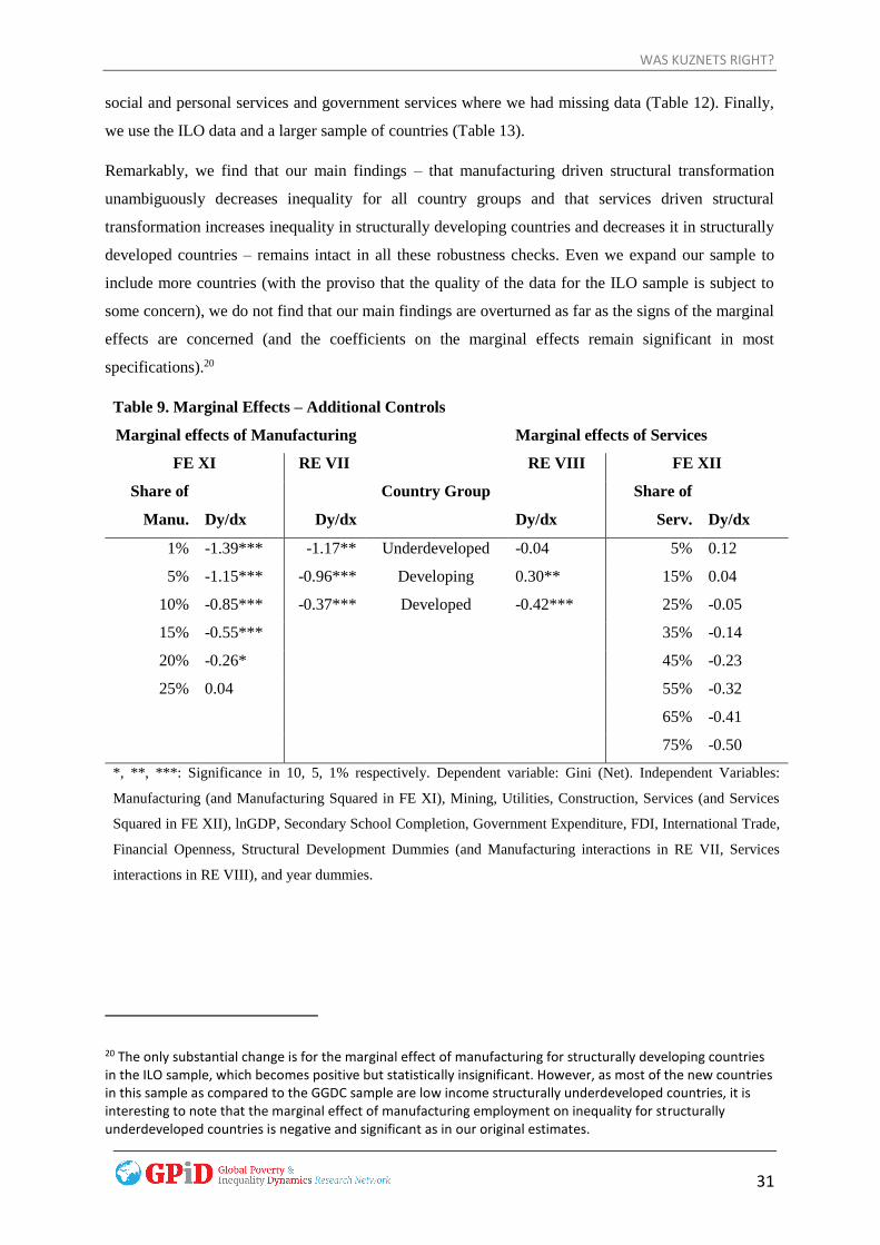
social and personal services and government services where we had missing data (Table 12). Finally,

we use the ILO data and a larger sample of countries (Table 13).

Remarkably, we find that our main findings – that manufacturing driven structural transformation

unambiguously decreases inequality for all country groups and that services driven structural

transformation increases inequality in structurally developing countries and decreases it in structurally

developed countries – remains intact in all these robustness checks. Even we expand our sample to

include more countries (with the proviso that the quality of the data for the ILO sample is subject to

some concern), we do not find that our main findings are overturned as far as the signs of the marginal

effects are concerned (and the coefficients on the marginal effects remain significant in most

specifications).20

Table 9. Marginal Effects – Additional Controls

Marginal effects of Manufacturing Marginal effects of Services

FE XI RE VII RE VIII FE XII

Share of

Manu.

Dy/dx

Dy/dx

Country Group

Dy/dx

Share of

Serv.

Dy/dx

1% -1.39*** -1.17** Underdeveloped -0.04 5% 0.12

5% -1.15*** -0.96*** Developing 0.30** 15% 0.04

10% -0.85*** -0.37*** Developed -0.42*** 25% -0.05

15% -0.55*** 35% -0.14

20% -0.26* 45% -0.23

25% 0.04 55% -0.32

65% -0.41

75% -0.50

*, **, ***: Significance in 10, 5, 1% respectively. Dependent variable: Gini (Net). Independent Variables:

Manufacturing (and Manufacturing Squared in FE XI), Mining, Utilities, Construction, Services (and Services

Squared in FE XII), lnGDP, Secondary School Completion, Government Expenditure, FDI, International Trade,

Financial Openness, Structural Development Dummies (and Manufacturing interactions in RE VII, Services

interactions in RE VIII), and year dummies.

20 The only substantial change is for the marginal effect of manufacturing for structurally developing countries in the ILO sample, which becomes positive but statistically insignificant. However, as most of the new countries in this sample as compared to the GGDC sample are low income structurally underdeveloped countries, it is interesting to note that the marginal effect of manufacturing employment on inequality for structurally underdeveloped countries is negative and significant as in our original estimates.

WAS KUZNETS RIGHT?

32

Table 10. Marginal Effects – Gross Gini

Marginal effects of Manufacturing Marginal effects of Services

FE XIII RE IX RE X FE XIV

Share of

Manu.

Dy/dx

Dy/dx

Country Group

Dy/dx

Share of

Serv.

Dy/dx

1% -0.71** -0.87** Underdeveloped -0.04 5% -0.00

5% -0.62** -0.43* Developing 0.30** 15% -0.09

10% -0.52*** -0.26*** Developed -0.42*** 25% -0.18

15% -0.41*** 35% -0.26*

20% -0.30*** 45% -0.35**

25% 0.19* 55% -0.44**

65% -0.52**

75% -0.61**

*, **, ***: Significance in 10, 5, 1% respectively. Dependent variable: Gini (Gross). Independent Variables:

Manufacturing (and Manufacturing Squared in FE XIII), Mining, Utilities, Construction, Services (and Services

Squared in FE XIV), lnGDP, Secondary School Completion, Government Expenditure, Structural Development

Dummies (and Manufacturing interactions in RE IX, Services interactions in RE X), and year dummies.

Table 11. Marginal Effects – Sample excluding Rich Countries

Marginal effects of Manufacturing Marginal effects of Services

FE XV RE XI RE XII FE XVI

Share of

Manu.

Dy/dx

Dy/dx

Country Group

Dy/dx

Share of

Serv.

Dy/dx

1% -1.06*** -1.41 Underdeveloped -0.04 5% -0.05

5% -0.90*** -1.31*** Developing 0.30** 15% -0.10

10% -0.71*** -0.38 Developed -0.42*** 25% -0.15

15% -0.51*** 35% -0.20

20% -0.31*** 45% -0.25

25% -0.12 55% -0.30*

65% -0.35*

75% -0.40*

*, **, ***: Significance in 10, 5, 1% respectively. Dependent variable: Gini (Net). Independent Variables:

Manufacturing (and Manufacturing Squared in FE XV), Mining, Utilities, Construction, Services (and Services

Squared in FE XVI), lnGDP, Secondary School Completion, Government Expenditure, Structural Development

Dummies (and Manufacturing interactions in RE XI, Services interactions in RE XII), and year dummies.

WAS KUZNETS RIGHT?

33

Table 12. Marginal Effects – Full GGDC Sample with Imputations

Marginal effects of Manufacturing Marginal effects of Services

FE XVII RE XIII RE XIV FE XVIII

Share of

Manu.

Dy/dx

Dy/dx

Country Group

Dy/dx

Share of

Serv.

Dy/dx

1% -0.60* -1.47*** Underdeveloped -0.11 5% 0.18

5% -0.53** -0.11 Developing 0.19* 15% 0.10

10% -0.45** -0.24*** Developed -0.09 25% 0.02

15% -0.36*** 35% -0.06

20% -0.27*** 45% -0.14

25% -0.19** 55% -0.22*

65% -0.30*

75% -0.38*

*, **, ***: Significance in 10, 5, 1% respectively). Dependent variable: Gini (Net). Independent Variables:

Manufacturing (and Manufacturing Squared in FE XVII), Mining, Utilities, Construction, Services (and Services

Squared in FE XVIII), lnGDP, Government Expenditure, Structural Development Dummies (and Manufacturing

interactions in RE XIII, Services interactions in RE XIV), and year dummies.

Table 13. Marginal Effects – ILO and GGDC Sample

Marginal effects of Manufacturing Marginal effects of Services

FE XIX RE XV RE XVI FE XX

Share of

Manu.

Dy/dx

Dy/dx

Country Group

Dy/dx

Share of

Serv.

Dy/dx

1% -0.52** -1.00** Underdeveloped -0.27 5% 0.13

5% -0.44** 0.03 Developing 0.12 15% 0.08

10% -0.36*** -0.20*** Developed -0.06 25% 0.03

15% -0.28*** 35% -0.01

20% -0.19*** 45% -0.06

25% -0.11* 55% -0.11*

65% -0.16

75% -0.20

*, **, ***: Significance in 10, 5, 1% respectively). Dependent variable: Gini (Net). Independent Variables:

Manufacturing (and Manufacturing Squared in FE XIX), Mining, Utilities, Construction, Services (and Services

Squared in FE XX), lnGDP, Government Expenditure, Structural Development Dummies (and Manufacturing

interactions in RE XV, Services interactions in RE XVI), and year dummies.

WAS KUZNETS RIGHT?

34

7. Conclusions

Structural transformation is at the core of the process of economic development. While a rapid pace of

structural transformation can lead to sustained economic growth, it can contribute to growing inequality,

as had been suggested by Kuznets. In this paper, we examine whether structural transformation leads to

higher inequality. We first document the very different paths of structural transformation that different

countries have followed in the past five decades. Countries show different paths of structural

transformation, being either structurally under-developed, structurally developing or structurally

developed. We then investigate whether these different paths of structural transformation have had

differential impacts on inequality, using a panel of developing and developed countries for the period

1960-2012. In contrast to the Kuznets hypothesis, we find that the movement of workers to

manufacturing unambiguously decreases income inequality, irrespective of the stage of structural

transformation that a particular country is in. We also find that while the movement of workers into

services has no discernible overall impact on inequality across our set of countries, there is clear

heterogeneity in the impact of services driven structural transformation on inequality. In particular, we

find that structural transformation relating to services increases inequality in structural developing

countries and decreases inequality in structurally developed countries. Thus, our findings suggest that

the Kuznets postulate seems to apply more to services than to manufacturing driven structural

transformation.

A large literature has previously documented the beneficial effects that manufacturing driven structural

transformation can have on the economic development process through its positive effect on sustained

economic growth and productive job creation (e.g., Rodrik 2013, UNIDO 2013, Felipe et al. 2015). In

this paper, we establish another mechanism by which manufacturing can be beneficial to development

– employment creation in manufacturing can reduce overall inequality as well. This suggests a double

dividend of manufacturing driven structural transformation - through increased growth and reduced

inequality. However, for the vast majority of low income countries which would fall into the structurally

underdeveloped category, the data suggests that the prospects for a manufacturing driven structural

transformation seem unlikely. For these countries, where the realistic possibility of structural

transformation is the movement of workers from agriculture to services, our findings suggest that for

these countries, inequality will increase with further structural transformation.

WAS KUZNETS RIGHT?

35

References:

Acemoglu, D. and J.A. Robinson (2002). The Political Economy of the Kuznets Curve. Review of

Development Economics, 6(2), pp. 183-2002.

Anand, S. and Kanbur, S.R., 1993a. The Kuznets process and the inequality—development

relationship. Journal of development economics, 40(1), pp.25-52.

Anand, S. and Kanbur, S.R., 1993b. Inequality and development A critique. Journal of Development

economics, 41(1), pp.19-43.

Angeles, L., 2009. An alternative test of the Kuznets’ hypothesis. Journal of Economic Inequality, 8(4),

pp. 463-473.

Baymul, C. and Shorrocks, A. (2018). World Income Inequality Dataset 4, Forthcoming.

Castello-Climent, A and R Doménech (2014), “Human Capital and Income Inequality: Some Facts

and Some Puzzles”, BBVA Research Working Paper 12/ 28.

Chinn, M. D. and H. Ito (2006). "What Matters for Financial Development? Capital Controls,

Institutions, and Interactions," Journal of Development Economics, 81(1), pp. 163-192.

Dabla-Norris, E., Thomas, A.H., Garcia-Verdu, R. and Chen, Y., 2013. Benchmarking structural

transformation across the world. IMF Working Paper.

Dabla-Norris, M.E., Kochhar, M.K., Suphaphiphat, M.N., Ricka, M.F. and Tsounta, E., 2015. Causes

and consequences of income inequality: a global perspective. International Monetary Fund.

Diao, X., McMillan, M. and Rodrik, D., 2017. The recent growth boom in developing economies: A

structural change perspective (No. w23132). National Bureau of Economic Research.

Duarte, M. and Restuccia, D., 2010. The role of the structural transformation in aggregate

productivity. The Quarterly Journal of Economics, 125(1), pp.129-173.

Felipe, J., Mehta, A. and Rhee, C., 2015. Manufacturing matters… but it's the jobs that count.

Economics and Research Department Working Paper # 420, Asian Development Bank, Metro Manila.

Galbraith, J. K., B. Halbach, A. Malinowska, A. Shams and W. Zhang (2014). UTIP Global Inequality

Data-sets, 1963-2008: Updates, Revisions and Data Checks, UTIP Working Paper no. 68.

Goldberg, P K and N Pavcnik (2007). “Distributional Effects of Globalization in Developing

Countries”, Journal of Economic Perspectives, 45: 39–82.

Gollin, D., D. Lagakos and M.E. Waugh, 2014. The Agricultural Productivity Gap in Developing

Countries. Quarterly Journal of Economics 129(2): 939-993

WAS KUZNETS RIGHT?

36

Haraguchi, N., C.F.C. Cheng and E. Smeets (2017). “The Importance of Manufacturing in Economic

Development: Has This Changed?”, World Development, 93, 293-315.

Herrendorf, B., Rogerson, R. and Valentinyi, Á., 2014. Growth and Structural

Transformation. Handbook of Economic Growth, 2, pp.855-941.

Jaumotte, F., Lall, S. and Papageorgiou, C., 2013. Rising income inequality: technology, or trade and

financial globalization?. IMF Economic Review, 61(2), pp.271-309.

Kanbur, R., 2017. Structural Transformation and Income Distribution: Kuznets and Beyond. Charles H.

Dyson School of Applied Economics and Management, Cornell University, Working Paper no. 2017-

01.

Krueger, A.O., 1978. “Alternate Trade Strategies and Employment in LDCs”, American Economic

Review, May: 270-274.

Krueger, A.O., 1980. Trade and Employment in Developing Countries: Synthesis and Conclusion,

Chicago: University of Chicago Press.

Kuznets, S., 1955. Economic growth and income inequality. The American economic review, pp.1-28.

Kuznets, S. and Murphy, J.T., 1966. Modern economic growth: Rate, structure, and spread (Vol. 2).

New Haven: Yale University Press.

Lewis, W.A., 1954. Economic development with unlimited supplies of labour. The manchester

school, 22(2), pp.139-191.

Lindert, P.H. and Williamson, J.G., 2003. Does globalization make the world more unequal?.

In Globalization in historical perspective (pp. 227-276). University of Chicago Press.

McMillan, M., Rodrik, D. and Verduzco-Gallo, Í., 2014. Globalization, structural change, and

productivity growth, with an update on Africa. World Development, 63(1), pp.11-32.

Milanović, B., 2000. Determinants of cross-country income inequality: An ‘augmented’Kuznets

hypothesis. In Equality, Participation, Transition (pp. 48-79). Palgrave Macmillan UK.

Riedel, J., 1988. “Economic Development in East Asia: Doing What Comes Naturally?”, in H. Hughes

(ed.), Achieving Industrialisation in East Asia, Cambridge: Cambridge University Press.

Robinson, S., 1976. A Note on the U Hypothesis Relating Income Inequality and Economic

Development. American Economic Review, 66(3), pp. 437-440.

Rodrik, D., 2013. Unconditional Convergence in Manufacturing. Quarterly Journal of Economics. Vol.

128 (1), pp.165-80.

WAS KUZNETS RIGHT?

37

Roine, J. and Waldenström, D., 2015. Long-run trends in the distribution of income and wealth. In The

Handbook of Income Distribution 2, San Diego: Elsevier.

Sumner, A., 2017. “The Developer’s Dilemma: The Inequality Dynamics of Structural Transformation

and Inclusive Growth”, Working Paper No. 1, Global Poverty and Inequality Dynamics Research

Network, https://www.gpidnetwork.org/research/.

Timmer, M.P. and de Vries, G.J., 2009. Structural change and growth accelerations in Asia and Latin

America: a new sectoral data set. Cliometrica, 3(2), pp.165-190.

Timmer, M. P., de Vries, G. J., & de Vries, K., 2015. “Patterns of Structural Change in Developing

Countries.” . In J. Weiss, & M. Tribe (Eds.), Routledge Handbook of Industry and Development. (pp.

65-83). Routledge.

UNIDO (2013). Sustaining Employment Growth: The Role of Manufacturing and Structural Change,

Industrial Development Report 2013, Geneva: UNIDO.

Wood, A. 2017. Variation in structural change around the world, 1985-2015. WIDER Working Paper

2017/34.

World Bank, 2017. Trouble in the Making? The Future of Manufacturing-Led Development. The World

Bank, Washington D.C.

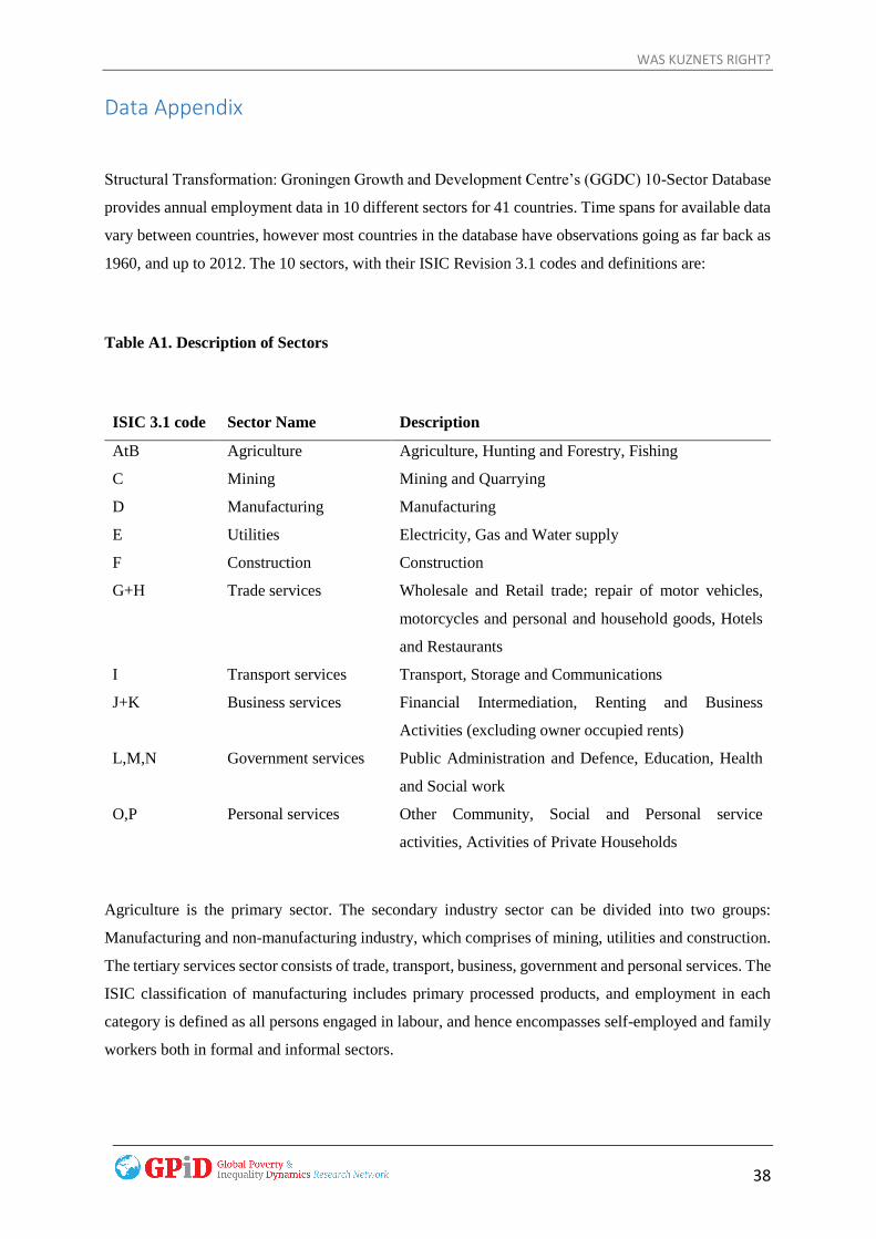
WAS KUZNETS RIGHT?

38

Data Appendix

Structural Transformation: Groningen Growth and Development Centre’s (GGDC) 10-Sector Database

provides annual employment data in 10 different sectors for 41 countries. Time spans for available data

vary between countries, however most countries in the database have observations going as far back as

1960, and up to 2012. The 10 sectors, with their ISIC Revision 3.1 codes and definitions are:

Table A1. Description of Sectors

ISIC 3.1 code Sector Name Description

AtB Agriculture Agriculture, Hunting and Forestry, Fishing

C Mining Mining and Quarrying

D Manufacturing Manufacturing

E Utilities Electricity, Gas and Water supply

F Construction Construction

G+H Trade services Wholesale and Retail trade; repair of motor vehicles,

motorcycles and personal and household goods, Hotels

and Restaurants

I Transport services Transport, Storage and Communications

J+K Business services Financial Intermediation, Renting and Business

Activities (excluding owner occupied rents)

L,M,N Government services Public Administration and Defence, Education, Health

and Social work

O,P Personal services Other Community, Social and Personal service

activities, Activities of Private Households

Agriculture is the primary sector. The secondary industry sector can be divided into two groups:

Manufacturing and non-manufacturing industry, which comprises of mining, utilities and construction.

The tertiary services sector consists of trade, transport, business, government and personal services. The

ISIC classification of manufacturing includes primary processed products, and employment in each

category is defined as all persons engaged in labour, and hence encompasses self-employed and family

workers both in formal and informal sectors.

WAS KUZNETS RIGHT?

39

Appendix A2: Alternate Sources of Employment Data

There are two additional sources for data, apart from the GGDC database, on sectoral employment at

the country level. The first is World Bank’s World Development Indicators (WDI), which covers more

countries than the GGDC. However, the WDI only reports total share of labour in agriculture, industry

and services. The industry sector consists of mining, construction, public utilities and manufacturing,

while the services sector consists of wholesale and retail trade and restaurants and hotels; transport,

storage, and communications; financing, insurance, real estate, and business services; and community,

social, and personal services. The WDI data-set does not break down industry employment data by

manufacturing and non-manufacturing (mining, construction, utilities) and services employment by

sub-sectors. The aim of our analysis is to examine the impact of manufacturing as well as service sub-

sectors on inequality. Since WDI does not offer information on sub-sectoral allocations of employment,

we are unable to use the data they provide.

A second source of employment data is the International Labour Organisation’s ILOSTAT database.

ILOSTAT provides detailed information on the number of people working in each sector, for majority

of the countries since 1950s. The data is based mostly on labour force surveys and supplemented by

censuses and other minor sources. However, even though ILOSTAT offers the largest sample size and

time scale, comparability of this dataset is limited as concept definitions and population coverage differ

between countries and over time. The frequency of the data collected also varies between countries and

disregard all impacts of seasonality on the labour force. For these reasons, the GGDC 10-Sector dataset

is our preferred data source. Nevertheless, we use the available ILOSTAT data as a robustness check

since it vastly increases our sample size.

WAS KUZNETS RIGHT?

40

Appendix A3. Control Variables

Economic Development: The natural logarithmic values of Gross Domestic Product (GDP) per capita

in 2011 US Dollars taken from the Penn World Table 9.0 are used to proxy economic development of

countries.

Human Capital: Percentage of people aged 15 and over who completed secondary school is the

preferred proxy to control for the level of human capital endowment in countries. Data is taken from

the Barro-Lee Educational Attainment Dataset.

Government Expenditure: Government expenditure is the final government consumption expenditure

as a share of the total GDP. Data for Taiwan is taken from the National Statistics Agency’s website,

while data for the rest of the countries are provided by the World Development Indicators of the World

Bank.

In order to obtain consistent and comparable results between our regression estimates, we only include

observations without any missing values for any of our dependent or independent variables. Doing so

generates an unbalanced panel dataset that consists of 29 countries, with 5-year averaged periods

between 1960 and 2012. Only Japan, the United Kingdom and the United States have data for all the 11

periods, while Malawi has the least number of observations, covering only four periods. Descriptive

statistics for the 219 observations for the 29 countries in the sample can be seen in Table 1. It

demonstrates that the countries in our sample differ widely in their macroeconomic characteristics and

structural composition. The share of employment in agriculture, an indicator for economic development,

has a standard deviation of 24%, with a minimum and maximum range of 0.2% to 87%.