Wal-Mart’s Monopsony Power in Local Labor Markets

Alessandro Bonanno and Rigoberto A. Lopez

Assistant Professor in Residence and Professor, respectively Department of Agricultural and Resource Economics,

University of Connecticut, 1376 Storrs Road, Storrs, CT 06269-4021, Corresponding author: Alessandro Bonanno, Phone (860)-486-1923, Fax: (860)-486-1932,

Email alessandro.bonanno@uconn.edu

Selected Paper prepared for presentation at the American Agricultural Economics Association Annual Meeting, Orlando, FL, July 27-29, 2008.

Copyright 2008 by A. Bonanno and R. A. Lopez. All rights reserved. Readers may make verbatim copies of this document for non-commercial purposes by any means, provided that this copyright notice appears on all such copies.

1

JEL: J42, L13, L81

Wal-Mart’s Monopsony Power in Local Labor Markets**

Abstract

This paper measures the degree of monopsony power exerted by Wal-Mart over retail workers

using a dominant-firm model and data on contiguous U.S. counties where the company operates,

presenting for the first time a measure of the anti-competitive behavior of the company.

Empirical results show that Wal-Mart’s monopsony power over workers varies significantly

across the country, being higher in rural counties, particularly in the south. For instance, Wal-

Mart’s buying power index in labor markets in rural southern central states is estimated to be 5%

or higher while the impact on northeastern states’ retail wages is negligible.

** The authors would like to thank Ronald W. Cotterill, Xenia Matschke, Delia Furtado, Elena

Lopez and Emek Basker for valuable comments and suggestions during the development of this

paper. All remaining errors are, of course, the responsibility of the authors.

2

Introduction

Wal-Mart, the largest retailer in the world, employs nearly 1.4 million people in the

United States (Wal-Mart Inc. United States Operational Datasheet, May 2007), making it the

largest private employer. The growth of Wal-Mart in the last two decades, fueled by low

consumer prices and costs,1 has significantly altered the retailing and employment landscape

throughout the country. Moreover, Wal-Mart has been the target of local and state regulation

proposals of numerous lawsuits regarding its workforce. Critics contend that the company

undercuts wages. However, only mixed empirical evidence exists to support this claim.

From an economic standpoint, lower wages can be due to companies’ buying power,

productivity of non-labor inputs, and strategic location in lower-wage markets. The available

literature has focused on controlling for the latter without relying on a structural model that

explicitly accounts for the sources of the company’s lower wages, leaving interpretation hostage

to empirical results. The benchmark for comparison has so far been wages in counties where

Wal-Mart does not operate, which does not necessarily reflect the competitive benchmark once a

Wal-Mart has located there.

The empirical evidence is also scant and rather mixed: Ketchum and Hughes (1997) find

no evidence of Wal-Mart's impact on wage growth and employment across Maine counties.

Neumark, Zhang and Ciccarella (2006) find a negative impact of Wal-Mart on per capita

earnings, estimated at an approximately 2.7% drop per store opening. Dube, Lester and Eidlin

(2007) find a negative impact on retail earnings estimated to be between 0.5 and 0.9%.2 Basker

(2005a) finds instead Wal-Mart having small positive effect on county-level retail employment,

even if reducing wholesale employment.

3

Table 1 illustrates the importance of Wal-Mart in U.S. retail labor markets.3

Overall, Wal-Mart has a higher share of retail employment in the south and mid-west, where it

typically employs one in four or five retail workers in the counties where it operates, than in the

northeast or the Pacific west. Wal-Mart has not only faced myriad labor lawsuits but also policy

maker's threats in Illinois and Maryland. A Chicago City Council ordinance, successively vetoed

by the Mayor, required stores with more than 90,000 square feet and companies grossing more

than $1 billion annually to pay a hourly minimum wage of $10 and benefits worth at least $3.

The Maryland State Assembly passed the Maryland Fair Share Health Act which would have

imposed tax burdens on companies paying low healthcare benefits, which, by design, was to

affect only Wal-Mart, violating federal trade laws (Wagner, 2006). Being notoriously a “union-

free” company, Wal-Mart also faces stiff criticism by public officials and labor unions: in

February 2004, democratic Congressman George Miller presented a report to the House of

Representative highlighting the low-wage and union-free policies of the company and the many

labor malpractice which Wal-Mart stores’ managers are allegedly responsible for (Miller, 2004).

In other words, the company has faced nationwide criticism regarding labor wages and

conditions, regardless of its importance in local labor markets and without well-grounded

economic evidence.

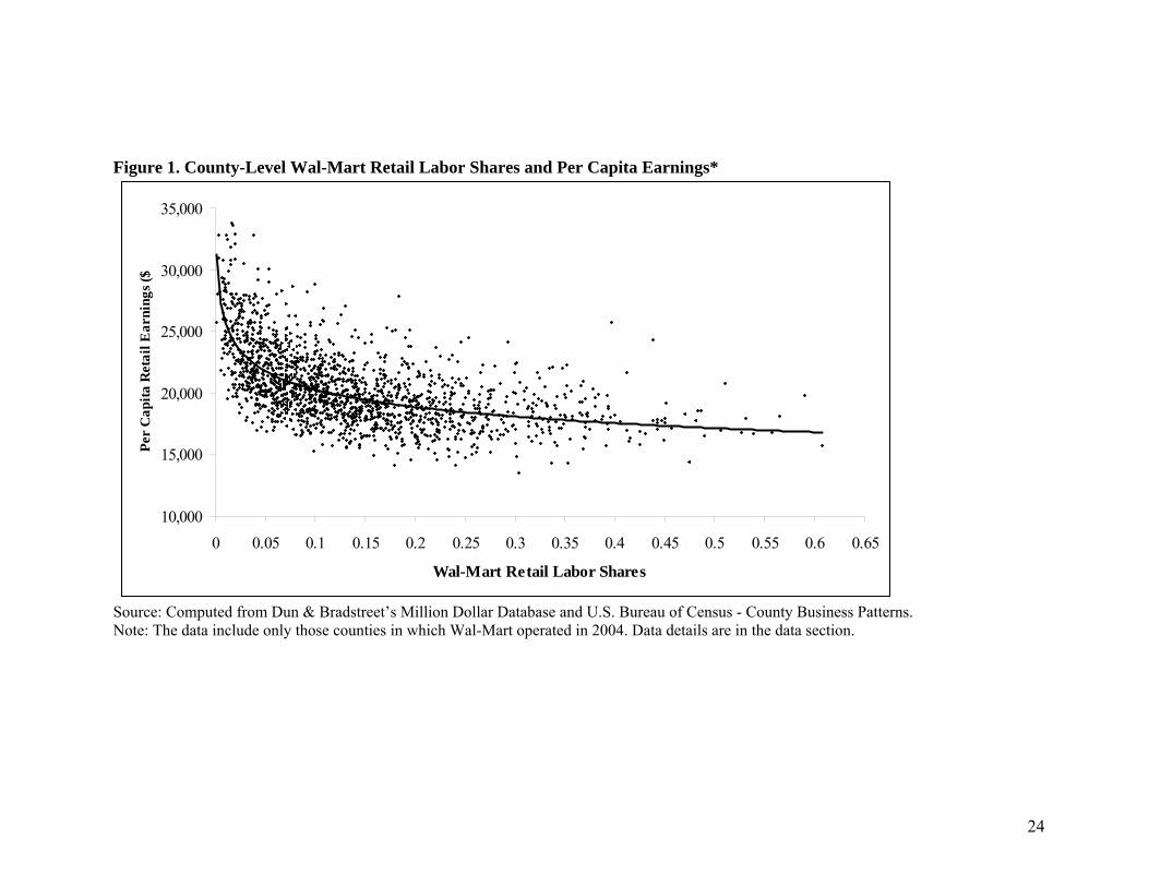
Figure 1 illustrates the correlation between Wal-Mart retail labor shares and average

retail labor earnings in counties where the company operated in 2004. It is interesting to note that

higher Wal-Mart labor shares in those counties are associated with lower workers’ earnings,

suggesting a wage-decreasing effect. However, this is not evidence of exploitation as these

figures do not correct for local market conditions or productivity differentials and do not

consider the presence of monopsony power markdown. Given the public concern over the

4

impact of the company on retail workers and the existence of competing explanations for its

alleged wage-decreasing effects, there is a need for formal structural analysis that quantifies the

effect, rigorously testing for the hypothesis of monopsony power over workers based on local

rather than nationwide conditions.

This paper estimates a structural framework to measure Wal-Mart’s monopsony power in

local labor markets. A dominant firm model is estimated with data from contiguous U.S.

counties where Wal-Mart operated in 2004. Empirical results show that although Wal-Mart’s

monopsony power is on average limited (less than 3%), the company exerts a significant amount

of power over workers in rural areas located in south central states where it consistently exceeds

5%, generating concerns in terms of workers’ losses. On the other hand, Wal-Mart effect on

retail earnings in the northeast is practically negligible. While we find evidence to support the

criticisms in some states, the findings do not support the notion that this is a nationwide problem.

The Model

Consider a simple dominant firm model with labor as the only variable input, where Wal-

Mart exerts monopsony power in the labor market. Wal-Mart sets wages at the level where the

marginal revenue product of labor (MRPLWM) equals marginal labor cost (mlc), which lies above

the company’s residual supply of labor ( sWMx , obtained by subtracting the fringe demand for labor

from the total supply of labor). This results in both a wage rate *x and an employment level *WMx

that are below the perfectly competitive ones ( pcw and pcWMx , respectively).4

To formalize, let ( ), TTX w Z and ( ),d d

FR FRx w Z represent the total supply of labor and

fringe demand for labor, where TZ and dFRZ are respectively vectors of total supply of labor and

5

fringe demand for labor shifters. Assuming no worker mobility across markets, the residual

supply of labor facing Wal-Mart ( WMx ) can be expressed as:

( ) ( ) ( ), , , , T d d T dWM T FR FR WM FRx X w Z x w Z x w Z Z= − = . (1)

For simplicity, assume that labor is homogenous and that it is the only variable input used

by Wal-Mart to sell a bundle of goods at competitive prices. The first-order condition for profit

maximization w.r.t. wages yields:

* (1 )WM WM WMw MRPL η η= + , (2)

where WMMRPL is the company’s marginal revenue product of labor and WMη is the wage

elasticity of the residual labor supply ( )ln lnWM WMx wη = ∂ ∂ . From (2), one can derive the

classical measure of monopsony power in labor markets, what Pigou (1924, p.754) defined as the

“rate of exploitation” and Blair and Harrison (1993) refer to as the Buying Power Index (BPI),

given by the inverse of the elasticity of the residual supply of labor facing Wal-Mart:

( )* * 1WM WMBPI MRPL w w η= − = . (3)

Given the assumption of homogeneous labor the residual supply of labor for Wal-Mart

can be obtained via the fringe demand for labor and total supply of labor.5 Using (1) and (3), the

BPI, representing Wal-Mart’s percent markdown below the marginal revenue product of labor is

given by:

(1 )dWM T FR WMBPI S Sη η⎡ ⎤= − −⎣ ⎦ , (4)

where WM WM TS x X= is Wal-Mart’s market share of the retailing labor market,

ln lnd dFR FRx wη = ∂ ∂ is the elasticity of the fringe demand for labor, and ln lnT TX wη = ∂ ∂ is the

6

elasticity of the total supply of labor for the retailing industry. In order to estimate BPI, one

needs values for both dFRη and Tη .

The total supply of retail labor is assumed to take a log-linear form given by

0ln lnT T l Tl TSl

X w Z eα η α= + + +∑ , (5)

where ln lnT TX wη = ∂ ∂ is the elasticity of the total supply of retailing labor, the ZTs are labor

supply shifters; the sα are parameters to be estimated; and eTS is an error term. The fringe revenue

function is assumed to be:

( )1 1FRFR FR FR FR FRR Z x kε γ ε+= + , (6)

where RFR represents revenues accruing to fringe retailers; 1 FRε+ the revenue elasticity with

respect to labor; and γ the revenue elasticity with respect to capital. For (6) to be well-behaved,

1 0FRε+ > or 1FRε > − , 0γ > and 1 0FRε γ+ + > . Under the assumption of a competitive fringe

(in the labor market), the wages offered will be equal to the marginal revenue product of labor:

FRFR FR FR FRw MRPL Z x kε γ= = (7)

Taking natural logs for both sides of the equations, rearranging and adding a random

error term, an estimable expression for the fringe retailers’ demand for labor is:

0ln ln lnd d dFR FR FR FR k FRk FD

k

x w k z eη η γ β β⎛ ⎞= − + + +⎜ ⎟⎝ ⎠

∑ , (8)

where ln is the natural log operator; ln lndFR FRx wη = ∂ ∂ is the elasticity of fringe demand,

which for consistency with (8) is expected to be less than 1< − (i.e., their demand for labor is

7

wage elastic);6 the skβ are parameters to be estimated; the dFRz s are labor demand shifters; and

eFD is an error term.

To complete the empirical model, one needs to address the issue that output, which is

usually introduced as a labor demand shifter, is potentially endogenous as addressed in Quandt

and Rosen (1989) and Gorter, Hassink, Nijkamp and Pels (1997). To deal with this problem,

output is modeled explicitly with an additional equation following Quandt and Rosen’s (1989)

approach. Using (8) and normalizing output prices to 1, an instrument for the log of output is

expressed as7

( )01ln ln 1 ln ln

FR

d d yFR FR FR FR FR FR l FRl FRp

ly R x k z eδ η η γ δ

=⎡ ⎤= = + + + + +⎣ ⎦ ∑ , (9)

where ( )0 ln 1 d dFR FRδ η η= − + and lnl FRl FR

lz Zδ =∑ ; the FRz s are output shifters; the sδ

parameters to be estimated and yFRe is an error term.

Summarizing, the model to be estimated consists of three simultaneous equations: total

supply of labor (equation 5), demand for labor by fringe retailers (equation 8), and an output

instrument (equation 9). From the estimated parameters, the monopsony power of Wal-Mart

over workers can be then obtained using equation (4).

Data and Estimation

Using the political boundaries of counties as the geographical definition of local markets,

the data used to estimate equations (5), (8) and (9) consisted of 1,607 contiguous U.S. counties in

which Wal-Mart operated in 2004. A total of 119 counties were excluded due to data disclosure

issues and missing observations. For the purposes of analysis, this sample (which will be referred

8

to as the “full sample”) was further sub-divided into 746 urban and 861 rural counties, using the

U. S. Bureau of Census classification system.8 Wal-Mart employment at the country level came

from aggregating individual store employment data from Dun & Bradstreet’s Million Dollar

Database (D&B).9 Total county retail employment (NAICS 44) and earnings came from the

County Business Patterns (CBP) database of the U.S. Bureau of Census, excluding Motor

Vehicles and Parts Dealers (NAICS 441). The values for NAICS 441 (Motor Vehicle and Parts

Dealers) were subtracted from the total, given that Wal-Mart does not compete directly with

those types of businesses and that workers in this sub-industry have skills that cannot be easily

transferred to other businesses. NAICS 441 is also one of the excluded sub-industries in Basker

(2005a). Then Wal-Mart’s shares of retail employment and average retail earnings (used in lieu

of wages) were computed. State averages are shown in Table 1 along with the number of Wal-

Mart stores in each state.

For equation (5), the dependent variable is total county retail employment discussed

above. The supply shifters are: total size of the labor force, unemployment rate,10 state-level

personal income tax rate, following the disequilibrium model of Hall, Henry and Pemberton

(1992), earnings for other low-skilled jobs (measured by the per capita earnings for the NAICS

722 industry: Food Services and Drinking Places), and composition of the labor force, as in

Dube et al., (2007). The last includes the percentages of the eligible population that are female,

white Caucasian, and belonging to the three age groups 15-24, 25-64 and over 65 years of age.

County labor force data including total labor force and unemployment rate are retrieved from the

U.S. Bureau of Census County Population Survey, while county-level population characteristics

are retrieved from the Population Estimates Program. The same source is used to obtain the

percentage of population above 25 years of age having at least a high school degree, which is

9

used as proxy for education level. Per capita earnings for the NAICS 722 (Food Services and

Drinking Places) are obtained from the CBP and used as proxy for earnings of other low-skill

jobs.

For equation (8), the dependent variable is total retail employment minus Wal-Mart’s.

The fringe demand shifters are: capital investment (measured by the number of fringe stores per

square mile), the number of years Wal-Mart operated in a county (to capture strategic and any

technological changes due to the company’s presence; see Khanna and Tice, 2000) from Emek

Basker’s Wal-Mart store openings database, the state-level percentage of unionized workers

(from the Bureau of Labor Statistics multiplied by county-level retail employment), and output.

Equation (9) is estimated to instrumentalize fringe output. The dependent variable is sales

data for retail establishments (excluding NAICS 441) from the Economic Census for 2002,

projected to 2004 values, using the percentage growth of the retail trade contribution to the Gross

State Product (U.S. Bureau of Economic Analysis) from 2002 to 2004, minus Wal-Mart sales

obtained from D&B. Partial productivity of retail labor is measured by dividing retail gross

product11 by the total number of retail workers in each county.

In order to account for the fact that the markdown is determined by the monopsonist’s

market share, as in equation (3), the natural log of earnings is w is regressed on a set of

exogenous variables that are correlated with Wal-Mart’s presence across different geographic

areas, such as county population density, distance from Benton County12 (measured in hundreds

of miles and is obtained applying the Haversine formula to county coordinates obtained from the

Census Gazetteer of Counties for the year 2000), its squared value and Census division13

dummies. The predicted log of earnings is then used in place of the actual ones in the system.14

10

All variables used as shifters are expressed in natural log values unless otherwise

specified. Also, in order to control for unobservables, the shifters of all equations include fixed

regional effects (i.e., dummies for eight out of the nine Census divisions).

Once all the variables were operational, equations (5), (8) and (9) were estimated

simultaneously via heteroscedastic robust non-linear three stage least squares. Three versions of

the model were estimated: the full sample (with 1,607 observations), rural counties, and urban

counties. The results are presented below.

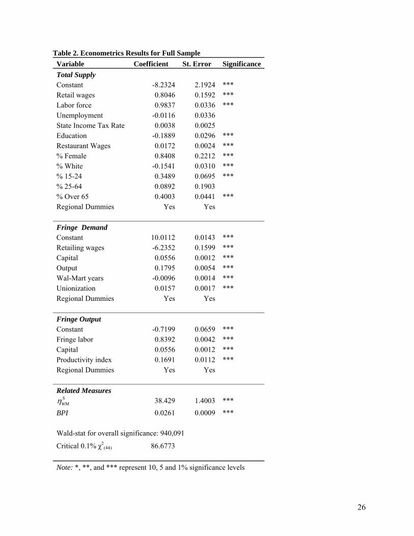
Empirical Results The parameter estimates and the associated statistics using the full sample are presented

in Table 2. Nearly all the parameters are statistically significant at the 1% level and show the

expected signs. Furthermore, the Wald test for joint significance of the model shows significance

at the 0.1%.

The elasticity of retail labor supply with respect to wages is approximately 0.80,

indicating a moderate responsiveness of workers to wages. In terms of shifters, the results are

consistent with the composition of the population willing to work in the retailing industry (see

Dube et al. 2007): higher education makes individuals less likely to supply labor to this industry

as is being white Caucasian, while females and those in age groups including high school/college

students (15-24) and retirees (over 65) are more likely to actively seek jobs in retailing, being

also more willing to accept part time jobs and the flexibility required by retailing jobs. Also,

restaurant workers’ earnings are positively related to the supply of labor in retailing; however,

the small estimated coefficient suggests a limited complementarity between the two types of

11

low-skill jobs.15 The retailing supply of labor is not significantly affected by state income tax or

unemployment rates.

The wage elasticity of the fringe demand for labor is estimated at approximately -6.23,

indicating that under monopsonistic wages, fringe retailers will tend to hire significantly more

retail workers countervailing in part employment losses from Wal-Mart’s anti-competitive

behavior. In terms of shifters, it can be pointed out that fringe retailers that have been exposed

longer to Wal-Mart tend to hire fewer workers. Considering that output is controlled for, this

suggests that the presence of Wal-Mart pushes its competitors toward labor-saving technologies.

Another possibility is that Wal-Mart expedites fringe retailers’ exit from or delays their entry

into the market, an effect that is absorbed in the coefficient of the output variable. In fact,

output, as reflected by fringe retail sales, significantly increases the fringe demand for labor,

while on the other hand, the degrees of capital utilization and unionization expand it. While the

first is a basic result from production theory, the second may be a result of surplus labor

generated by negotiation through unions. The estimated parameters for the fringe output

equation are significant and satisfy the restrictions of the theoretical model. Both the estimated

output elasticity of labor (0.8492) and capital (0.0556) are significant at the 1% level. As

expected, the partial productivity of labor increases output.

To gain further insight into Wal-Mart’s behavior in local labor markets, the model is

estimated separately for the two sub-samples, rural and urban areas. A Chow Test for structural

break in the parameters validates the hypothesis that the structure of the retailing labor market in

rural and urban counties is different.16 The parameter estimates and associated statistics are

presented in Tables 3 and 4.

12

The retailing supply of labor in urban areas is less elastic than in rural ones (0.4691 and

1.6127 respectively). This result indicates that workers in rural communities are more

responsive to changes in retail wages than urban workers, meaning that they are more willing to

supply labor to the retail industry as wages increase but also more easily discouraged by wage

decreases, making Wal-Mart’s wage decisions more crucial for rural areas. The other insight

from the two sets of estimates is that the age composition of the labor force matters. For

instance, in urban areas the retail labor supply is more strongly driven by the older (over 65) and

younger (15-24) population than in rural areas, where the main source of retail workers is those

in the 25-64 age range. This difference along with the fact that retail workers are less sensitive

to wage changes in urban than in rural areas indicates that retail jobs may be more appealing to

the workforce in those areas where there may be lack of employment alternatives.

The estimated fringe retailers’ demand for labor is more wage elastic in urban than in

rural counties, the estimated elasticities being approximately -6.09 and -4.41 respectively. This

implies that labor is a more important input for fringe retailers operating in rural areas than for

those operating in urban ones, which is also supported by the larger estimated parameters for

labor in the output equations.

In sum, what the split-sample regressions indicate is that the total supply of retail labor is

more sensitive to wages in rural counties than in urban ones while for the fringe demand the

wage-sensitivity is the reverse. These findings have direct implications for Wal-Mart’s residual

labor supply elasticity and therefore for the company’s monopsony power. From the estimated

parameters obtained for urban and rural counties, the market power of the company is expected

to be larger in the latter, regardless of the size of the market shares. As it can be seen from

equation (6) the larger the elasticity of the fringe demand, the smaller the magnitude of BPI;

13

being the demand for labor more elastic in urban areas than in rural areas, one would expect

Wal-Mart to have greater monopsony power in the latter. Although the magnitude of BPI

decreases with higher elasticities of supply (and the estimated elasticity of supply is lower in

urban than rural counties), the monopsony power of the company in rural areas will be larger

than in urban ones for all the values of labor shares included in the sample. This difference is

also expected to be exacerbated in many of the states because of the company’s large presence in

rural areas.

The buying power indexes are estimated in equation (6), using the econometric estimates

of the total labor supply elasticity and fringe demand elasticity with respect to wages and Wal-

Mart labor shares. As shown at the bottom of Tables 2-4, these estimates were highly significant.

For the full sample, the average residual supply elasticity facing Wal-Mart was estimated at

38.492, leading to a BPI of 2.61 %, indicating that nationally Wal-Mart pays wages that are

nearly 2.6% below their marginal revenue product of labor. Considering that the BPI provides an

upper bound to the percentage of wage decrease (the BPI would represent the effective

percentage decrease in earnings only if the monopsonist’s demand for the input was infinitely

elastic) this average result appears to be consistent with both Neumark et al.’s (2006) and Dube

et al.’s (2007) findings.

Considering that the Department of Justice does not have well-developed explicit

monopsony guidelines, applying a 5% rule (considered by the antitrust authorities in the

evaluation of market power in merger analysis as a “small but significant” level of market

power) as a threshold of imperfect competition, a 2.6% markdown on wages nationally does not

appear to be a compelling case for action against Wal-Mart by antitrust authorities or anti-Wal-

Mart organizations. However, for urban counties, Wal-Mart’s average residual supply of retail

14

labor is estimated at 54.48, resulting in a BPI of approximately 1.8%, while for the rural sample

Wal-Mart average residual supply elasticity is estimated at 25.656, leading to a BPI of

approximately 3.89%, larger than that of the total sample, and closer to the 5% threshold. Thus,

overall, the issue of monopsony power is less relevant in urban America, where Wal-Mart often

faces criticism for its labor practices.

Further insight is obtained when monopsony power is calculated by states, as shown in

Table 5. Given that the magnitude of BPI increases with the monopsonist’s market shares (Blair

and Harrison, 1993), Wal-Mart is expected to have significantly greater market power in

counties where it is the predominant employer in retailing. In fact, two consistent results are that

Wal-Mart shows larger market power in 1) rural counties than in urban ones, and 2) that in some

rural south-central states, the average BPIs exceed 5%. Thus rural counties in south-central

states, as well as in other selected states where the company’s presence is strong, are where Wal-

Mart monopsony power is the highest, exceeding 6% in Kansas, West Virginia and Arkansas,

and above 5% in five states (Colorado, Kentucky, Idaho, Illinois, Oklahoma and Utah). On the

other hand, counties in the Northeast, show minimal degrees of Wal-Mart’s monopsony power

over workers, with Vermont showing the lowest BPI among all states.

When examining individual states, it emerges that those areas where the company’s anti-

competitive behavior toward workers may raise concern, i.e. rural counties in south central and

north central states, do not necessarily coincide with areas where Wal-Mart’s labor practices are

strongly questioned. Of all the states where Wal-Mart has faced workers’ class actions,17 only

one present a BPI exceeding the 5% threshold in rural areas (Kentucky). Also, the estimated

BPIs do not support the necessity for policy intervention in Maryland (such as the Maryland Fair

Share Health Act) and urban Illinois (Chicago’s “living wage” ordinance).

15

Overall, the results presented in this paper do not support policy intervention aimed at

mitigating the company’s anti-competitive behavior for three reasons. First, given the small

magnitude of the wage-elasticity for the total supply of retailing labor and the large wage-

elasticity of fringe retailers’ demand for labor, the losses in workers’ surplus are likely to be

internalized in large part by firms operating in the market with relatively small deadweight

losses. Second, the measures presented here are valid for a post-entry scenario and do not

consider the overall impact of Wal-Mart’s entry on retail labor; there is no a priori reason to

believe that in counties without Wal-Mart, the perfectly competitive equilibrium wages paid by

other retailers would be higher than the monopsony wages set by the company. The same holds

for the level of retail employment, where the empirical evidence on the subject is mixed. Third,

considering Wal-Mart’s depressive impact on retail prices (Basker, 2005b; Basker and Noel,

2007; Hausman and Liebtag, 2005) and incumbent retailers’ oligopoly power (Cleary and Lopez,

2008), there are doubts as to whether deadweight losses from the company’s anti-competitive

behavior toward workers could overpower consumers’ welfare gains.

Concluding remarks

The vivid debate about the impact of Wal-Mart on retail workers’ conditions has

triggered an increasing number of studies, which have failed, however, to reach conclusive and

unanimous findings on the issue. This article estimates and tests for the degree of monopsony

power exerted by the company on local retail labor markets, using a dominant firm model and

data on contiguous U.S. counties.

Empirical results indicate that Wal-Mart does exert a statistically significant degree of

monopsony power over workers but that this varies significantly across the nation. Overall, the

16

average buying power index with respect to labor is approximately 2.6%, in line with some

previous findings. However, in selected rural areas of the south and the midwest, the degree of

Wal-Mart’s monopsony power reaches up to 6.4%, large enough to raise concerns.

Although this paper provides evidence of monopsonistic behavior by the company vis-à-

vis its workers in some areas, it fails to show evidence to warrant deeming this a nationwide

problem. In particular, the empirical evidence fails to show Wal-Mart having a consistently

large monopsonistic behavior in all the states where facing former workers’ class actions. Also,

those attempts to regulate the wage and benefit policies of the company by local governments in

Maryland and Illinois appear not to be justified from an economic standpoint. This leaves open

the question of why Wal-Mart workers’ issues are on local and state policy agendas throughout

the nation, especially in areas where there is no evidence of its monopsony power. The high

visibility of Wal-Mart makes it an easy target for policymakers and opinion leaders, who may

see attacking the company’s practices as a way to both increase public consensus and relieve

political pressure from interested parties (such as retail workers’ unions and traditional retailers).

17

Footnotes

1. For evidence of Wal-Mart’s beneficial impact on consumers through low prices, see for

instance Basker (2005b); Basker and Noel (2007); Cleary and Lopez (2008) and Hausman and

Liebtag (2005). Low costs have been attributed to an extremely efficient logistic system

(Edgecliffe–Johnson, 1999).

2. Interestingly, they established that Wal-Mart’s effect in decreasing earnings was not due to

differences in retailing workforce characteristics but was primarily associated with increased

rents for the company.

3. The relevant market consists in Retailing industry (NAICS 44) at the net of the Motor Vehicle

and Parts Dealers (NAICS 441) sub-industry; the data used to obtain the measures reported in

Table 1 and Figure 1 are described in the Data and Estimation section.

4. In this framework, the location of Wal-Mart is given. The resulting equilibrium wages and

employment if Wal-Mart was not present would be indicated by DFR =XT, which would result in

a lower wage than the monopsony one set by the company.

5. Under the assumption of heterogeneous labor, one could use the approach developed by Baker

and Bresnahan (1988). Even if this scenario would be more likely to represent a world in which a

firm, Wal-Mart, hires non-unionized workers and other firms are left to bargain wages with

unions, the unavailability of information on wages offered by both groups inhibits this approach.

6. Note that 1DFR FRη ε= ; therefore, in order to satisfy 1 0FRε+ > , the condition 1D

FRη < − needs to

hold.

7. This assumes that the bundles of goods sold are the same across counties. Although this is a

strong assumption, the unavailability of both retail quantity and price indexes at the county level

forces the use of a value measure in place of a quantity measure of output.

18

8. The U.S. bureau of Census classifies as “Metro” those areas including central counties with

urbanized areas of 50,000 or more residents, regardless of total area population, together with

outlying counties with commuting thresholds of 25 percent and as “rural” the remaining ones.

9. D&B gives information on each store’s type of business and location and estimates of its

number of employees and values of sales. Those estimates are obtained from different sources,

such as Government Registers and Legal Filing Offices and directly from the companies via

telephone surveys. Another feature of the D&B database that made the data collection a harder

process is that it is updated on a regular basis, so that historical data cannot be retrieved. To

obtain data for the stores operating in 2004 (the D&B data were retrieved in 2006), the stores

opened after December 2004 were excluded from the sample. Information on store opening was

found using Wal-Mart Inc. Website News section (www.walmartfacts.com ) and different years

of Wal-Mart’s shareholders’ Annual Reports.

10. Regarding the use of unemployment rate, although this is determined at the equilibrium in

the aggregate labor market, it is here considered exogenous in the determination of the market

clearing condition for one particular industry.

11. Adapting Bauer and Lee’s (2006) procedure to estimate the Gross State Product from

national data, the contribution to the GSP of each county is assigned in terms of the personal

income of the county population. Explicitly,

GCPi = GSP*PIi / PI,

where GCPi is the county-specific measure of value added; GSP is the Gross State Product for

the year 2004 from retail trade, obtained from the U.S. Bureau of Economic Analysis; and PIi

and PI are Personal Income at the county and state level respectively, also from the U.S. Bureau

of Economic Analysis.

19

12. Neumark et al. (2006) and Dube et al. (2007) use distance from Bentonville, Arkansas, and

time, to predict the timing of Wal-Mart entry. The idea of distance from Benton County,

Arkansas, being a good predictor of Wal-Mart’s presence in a county comes from Sam Walton’s

autobiography (Walton and Huey, 1992), in which it is explained how Wal-Mart bases its growth

strategy on expanding in areas closer to preexisting distribution centers, following the “hub and

scope” logistic system. Basker (2006), argues that the distance from Bentonville may not be a

good exogenous predictor of Wal-Mart expansion. However, given that this paper treats Wal-

Mart’s location as given, the distance from Benton County serves only the purpose of capturing

exogenous variation in the distribution of the number of stores across the continental U.S..

13. The U.S. Bureau of Census divides the national territory in four regions, which are further

divided in nine divisions. For a list of the regions, divisions and states they include, see Table 1.

14. The results of the OLS used to generate the instrument for the log of earnings are omitted for

brevity. However, the regression has an R-squared of 0.5217, only 3 of the variables are not

significant at the 10% level and an F-test for the joint significance of the parameters rejects the

null of non-significance at the 0.1% level.

15. Dube et al. (2007) found that restaurant workers per-capita earnings to be positively related

with retail workers’ earnings, but not in a statistically significant way.

16. The calculated F-statistic for the test is 3.0562, above the critical value at the 5% level (with

44 and 1519 degrees of freedom) of 1.3829 rejecting the null hypothesis of the two sub-samples

behaving in the same way.

17. The states that have been scenarios for Wal-Mart’s workers class actions against the

company are California, Georgia, Kentucky, Michigan, Missouri, New Jersey, New Mexico,

Oregon, Pennsylvania and Tennessee.

20

References

Baker, J. and T. F. Bresnahan, “Estimating the Residual Demand Curve Facing a Single Firm,”

International Journal of Industrial Organization, 6 (1988), 283–300.

Basker, E. “Wal-Mart Store Locations, 1972-2001 Database” Available at

http://web.missouri.edu/~baskere/data/ Accessed 10/06/2006.

Basker, E. “Job Creation or Destruction? Labor Market Effects of Wal-Mart Expansion” Review

of Economics and Statistics 87:1 (2005a), 174-183

Basker, E. “Selling a Cheaper Mousetrap: Wal-Mart's effect on retail prices,” Journal of Urban

Economics 58:2, (2005b) 203-229

Basker, E. “When Good Instruments Go Bad: A Reply to Neumark, Zhang and Ciccarella,”

University of Missouri Department of Economics Working Paper 07-06 (2006).

http://economics.missouri.edu/~baskere/papers/. Accessed 08/20/2007.

Basker, E. and M. Noel, “The Evolving Food Chain: Competitive Effects of Wal-Mart’s Entry

into the Supermarket Industry," University of Missouri Department of Economics

Working Paper 07-12 (2007). Available at

http://economics.missouri.edu/~baskere/papers/. Accessed 08/20/2007.

Bauer, P. W. and Y. Lee, “Estimating GSP and Labor Productivity by State”, Federal Reserve

Bank of Cleveland, Research Department, Policy Discussion Paper 16, (2006), Available

at www.clevelandfed.org/Research. Accessed 03/01/2007

Blair, R. D. and J. L. Harrison, “Monopsony: Antitrust Law and Economics” (Princeton, New

Jersey: Princeton University press, 1993).

Cleary, R.L.O. and R. A. Lopez, “Does the Presence of Wal-Mart Cause Dallas/Fort Worth

Supermarket Milk Prices to Become More Competitive?” Food Marketing Policy Center

21

Research Report, No. 99 (2008), Available at

http://www.fmpc.uconn.edu/publications/reports.php. Accessed 01/31/2008.

Dube, A., T. W. Lester, and B. Eidlin, “Firm Entry and Wages: Impact of Wal-Mart Growth on

Earnings throughout the Retailing Sector,” IRLE, University of California, Berkeley WP

iiwps-125-05 (2007). Available at http://www.irle.berkeley.edu/cwed/dube.html.

Accessed 12/17/2007.

Dun & Bradstreet’s Million Dollar Database (2006).

Edgecliff-Johnson, “A Friendly Store from Arkansas,” Financial Times (June 19, 1999).

Gorter, C., W. Hassink, P. Nijkamp and E. Pels, “On the Endogeneity of Output in Dynamic

Labour-Demand Models,” Empirical Economics, 22:3 (1997), 393-408.

Hall, S., G. B. Henry and M. Pemberton, “Testing a Discrete Switching Disequilibrium Model of

the UK Labor Market,” Journal of Applied Econometrics, 7:1 (1992), 83-91.

Hausman, J. and E. Leibtag, “Consumer Benefits from Increased Competition in Shopping

Outlets: measuring the Effect of Wal-Mart” NBER working paper series, No 11809

(2005). Available at http://www.nber.org/papers/w11809 . Accessed 06/10/2006.

Khanna, N. and S. Tice, “Strategic Responses of Incumbents to New Entry: The Effect of

Ownership Structure, Capital Structure, and Focus,” Review of Financial Studies, 13:3

(2000), 749-779.

Ketchum, B. and J. W. Hughes, “Wal-Mart and Maine: The Effect on Employment and Wages.”

Maine Business Indicators 42:3 (1997), 6-8.

Miller, George. “Every Day Low Wages: The hidden price we all pay for Wal-Mart” – Report by

the Democratic Staff of the Committee of Education and the Workforce – U.S. House of

22

the Representatives (February 16, 2004). Available at

http://www.wakeupwalmart.com/facts/miller-report.pdf Accessed 02/03/2008.

Neumark, D., J. Zhang and S. Ciccarella, “The Effects of Wal-Mart on Local Labor Markets,”

University of California-Irvine, Department of Economics Working Paper No.060711

(2006). Available at http://www.econ.uci.edu/docs/2006-07/Neumark-11.pdf Accessed

06/02/2007.

Pigou, A. C., The Economics of Welfare (London: Macmillan and Co, 1924).

Quandt, R.. and H. S. Rosen, “Endogenous Output in an Aggregate Model of the Labor Market”

The Review of Economics and Statistics, 71:3 (1989), 394-400.

U. S. Bureau of the Census, County Business Patterns (2004). Available at

http://www.census.gov/epcd/cbp/. Accessed06/20/2006.

U. S. Bureau of the Census, Current Population Survey (2004). Available at

http://www.census.gov/cps/. Accessed 07/16/2006.

U. S. Bureau of the Census: Economic Census (2002).

U. S. Bureau of the Census: Gazetteer of Counties (2000). Available at

http://www.census.gov/geo/www/gazetteer/places2k.html Accessed 06/20/2006.

U. S. Bureau of the Census, Population Estimates Program (2002-2004). Available at

http://www.census.gov/popest/estimates.php. Accessed 07/16/2006.

U. S. Bureau of Economic Analysis, Gross Domestic Product by State (2002-2004). Available at

http://www.bea.gov/regional/index.htm#gsp, acceded 03/20/2007.

U. S. Department of Agriculture, Economic Research Service ERS “Measuring Rurality: 2004

County Typology Codes” (2004).

23

Wagner, J. “MD. Legislature Overrides Veto on Wal-Mart Bill” The Washington Post, (January

13, 2006).

Wal-Mart Stores Inc. website www.walmartfacts.com/NewsRoom Accessed 07/08/2006.

Wal-Mart Stores Inc. (May 2007). United States Operational Data Sheet. Available at

http://www.walmartfacts.com/articles/5025.aspx . Accessed 16/07/2007

Wal-Mart Stores, Inc. (2001-2006). Shareholders’ Annual Reports. Available at

www.walmartstores.com Accessed 15/05/2007

Walton, S.. and J. Huey, “Sam Walton, Made in America: My Story”, (New York City:

Doubleday Publisher, 1992).

.

24

Figure 1. County-Level Wal-Mart Retail Labor Shares and Per Capita Earnings*

10,000

15,000

20,000

25,000

30,000

35,000

0 0.05 0.1 0.15 0.2 0.25 0.3 0.35 0.4 0.45 0.5 0.55 0.6 0.65

Wal-Mart Retail Labor Shares

Per

Cap

ita R

etai

l Ear

ning

s ($

Source: Computed from Dun & Bradstreet’s Million Dollar Database and U.S. Bureau of Census - County Business Patterns. Note: The data include only those counties in which Wal-Mart operated in 2004. Data details are in the data section.

25

Table 1. State Average Wal-Mart Retail Labor Shares (%), Retail Per-capita Earnings ($) and Number of Wal-Mart Stores, 2004.

Areas Retail Labor Shares

Per-Capita

Earnings

# Stores

Region Division State

Retail Labor Shares

Per-Capita

Earnings

# Stores

South West

West South Central Mountain Arkansas 26.07 16,675 70 Arizona 12.92 20,807 50Louisiana 17.66 17,294 74 Colorado 17.13 21,299 50Oklahoma 25.47 16,534 78 Idaho 17.65 19,844 15Texas 18.42 19,096 266 New Mexico 16.87 18,729 50East South Central Montana 9.87 19,245 10Alabama 17.76 18,456 82 Utah 16.08 18,177 26Kentucky 22.49 18,000 70 Nevada 15.43 22,333 20Mississippi 22.64 17,215 63 Wyoming 15.10 18,165 9Tennessee 19.16 19,029 85 Pacific South Atlantic California 5.84 23,624 135Delaware 7.82 21,624 8 Oregon 9.65 20,037 28Florida 12.85 20,261 155 Washington 10.53 20,765 31Georgia 16.44 19,662 103 Maryland 8.44 21,750 39 Midwest North Carolina 12.95 19,148 98 East North Central South Carolina 13.23 19,020 58 Indiana 17.57 17,704 86Virginia 19.06 18,975 27 Illinois 18.79 18,347 112West Virginia 22.30 17,500 29 Michigan 9.68 19,927 63 Ohio 11.08 18,809 98Northeast Wisconsin 10.41 17,790 66New England West North Central Connecticut 4.79 24,968 30 Iowa 15.47 17,945 52Maine 7.36 19,290 20 Kansas 23.64 16,840 47Massachusetts 4.14 23,332 42 Minnesota 10.03 18,200 44New Hampshire 8.31 22,820 25 Missouri 20.65 17,361 101Rhode Island 4.26 21,846 8 Nebraska 19.45 16,569 17Vermont 3.10 21,963 4 North Dakota 10.73 17,654 7Middle Atlantic South Dakota 13.34 17,516 7New Jersey 3.44 25,364 35 New York 8.93 19,812 77 Pennsylvania 8.89 18,881 94

Note: The state averages presented include only those counties where Wal-Mart operated in 2004. Source: Elaboration from Dun & Bradstreet’s Million Dollar Database; U.S. Bureau of Census - County Business Patterns; Wal-Mart Annual Report (2005).

26

Table 2. Econometrics Results for Full Sample Variable Coefficient St. Error SignificanceTotal Supply Constant -8.2324 2.1924 *** Retail wages 0.8046 0.1592 *** Labor force 0.9837 0.0336 *** Unemployment -0.0116 0.0336 State Income Tax Rate 0.0038 0.0025 Education -0.1889 0.0296 *** Restaurant Wages 0.0172 0.0024 *** % Female 0.8408 0.2212 *** % White -0.1541 0.0310 *** % 15-24 0.3489 0.0695 *** % 25-64 0.0892 0.1903 % Over 65 0.4003 0.0441 *** Regional Dummies Yes Yes Fringe Demand Constant 10.0112 0.0143 *** Retailing wages -6.2352 0.1599 *** Capital 0.0556 0.0012 *** Output 0.1795 0.0054 *** Wal-Mart years -0.0096 0.0014 *** Unionization 0.0157 0.0017 *** Regional Dummies Yes Yes Fringe Output Constant -0.7199 0.0659 *** Fringe labor 0.8392 0.0042 *** Capital 0.0556 0.0012 *** Productivity index 0.1691 0.0112 *** Regional Dummies Yes Yes Related Measures 38.429 1.4003 ***

BPI 0.0261 0.0009 *** Wald-stat for overall significance: 940,091

Critical 0.1% χ2(44) 86.6773

Note: *, **, and *** represent 10, 5 and 1% significance levels

SWMη

27

Table 3. Econometric Results for Urban Counties Variable Coefficient St. Error SignificanceTotal Supply Constant -4.0789 2.7844 Retail wages 0.4691 0.1874 ** Labor force 1.0403 0.0518 *** Unemployment 0.0553 0.0503 State Income Tax Rate 0.0046 0.0034 Education -0.2499 0.0339 *** Restaurants’ wages 0.0162 0.0048 ** % Female 1.0226 0.3881 ** % White -0.0973 0.0487 ** % 15-24 0.3858 0.0896 *** % 25-64 -0.5082 0.2578 ** % Over 65 0.3868 0.0538 *** Regional Dummies Yes Yes Fringe Demand Constant 10.0830 0.0183 *** Retailing wages -6.0949 0.2117 *** Capital 0.0667 0.0016 *** Output 0.1797 0.0075 *** Wal-Mart years -0.0094 0.0019 *** Unionization 0.0134 0.0023 *** Regional Dummies Yes Yes Output Constant -0.2359 0.1054 ** Fringe labor 0.8359 0.0051 *** Capital 0.0667 0.0016 *** Productivity index 0.0789 0.0169 *** Regional Dummies Yes Yes Related Measures 54.4830 2.7788 ***

BPI 0.01835 0.0009 ***

Wald-stat for overall significance: 496,241 Critical 0.1% χ2

(44) 86.6773 Note: *, **, and *** represent 10, 5 and 1% significance levels

SWMη

28

Table 4. Econometric Results for Rural Counties Variable Coefficient St. Error SignificanceTotal Supply Constant -18.1722 3.9524 *** Retail wages 1.6127 0.3134 *** Labor force 0.9849 0.04318 *** Unemployment -0.0519 0.0395 State Income Tax Rate 0.0010 0.0034 Education -0.1627 0.0408 *** Restaurant wages 0.0167 0.0026 *** % Female 1.2458 0.2567 *** % White -0.1445 0.0387 *** % 15-24 0.1503 0.0984 % 25-64 0.6198 0.2459 ** % Over 65 0.1552 0.0678 ** Regional Dummies Yes Yes Fringe Demand Constant 9.7968 0.0229 *** Retailing wages -4.4164 0.1718 *** Capital 0.0229 0.0017 *** Output 0.2883 0.0134 *** Wal-Mart years -0.0095 0.0015 *** Unionization 0.0128 0.0022 *** Regional Dummies Yes Yes Output Constant 0.0183 0.0884 Fringe labor 0.7735 0.0088 *** Capital 0.0229 0.0017 *** Productivity index 0.0417 0.0117 ** Regional Dummies Yes Yes Related Measures 25.656 1.7099 *** BPI 0.0389 0.0026 *** Wald-stat for overall significance: 781,998

Critical 0.1% χ2(44) 86.6773

Note: *, **, and *** represent 10, 5 and 1% significance levels

SWMη

29

Table 5. Estimated Buying Power Indexes: State Averages†

Areas All Urban Rural Region All Urban Rural

South Average BPIs West Average BPIs West South Central Mountain Arkansas 5.21 4.70 6.05 Arizona 2.30 1.28 3.77Louisiana 3.18 2.61 4.38 Colorado 3.30 1.07 5.43Oklahoma 5.33 5.40 5.91 Idaho 3.26 1.50 5.28Texas 3.38 2.52 4.67 New Mexico 2.87 1.03 3.87East South Central Montana 1.58 1.90 1.68Alabama 3.30 2.70 4.50 Utah 3.01 1.68 5.79Kentucky 4.48 2.99 5.56 Nevada 2.70 0.76 4.14Mississippi 4.40 5.51 4.60 Wyoming 2.55 1.44 3.27Tennessee 3.50 3.02 4.38 Pacific South Atlantic California 0.92 0.68 2.75Delaware 1.23 1.21 1.68 Oregon 1.58 1.01 2.29Florida 2.34 1.43 4.72 Washington 1.97 0.74 3.53Georgia 3.12 2.98 4.00 Maryland 1.43 1.13 2.83 Midwest North Carolina 2.23 2.02 2.84 East North Central South Carolina 2.36 2.08 3.13 Indiana 3.20 2.80 4.37Virginia 3.52 2.39 4.97 Illinois 3.75 2.77 5.03West Virginia 4.76 2.61 6.32 Michigan 1.62 0.91 2.77 Ohio 1.89 1.08 3.05Northeast Wisconsin 1.73 1.02 2.62New England West North Central Connecticut 0.72 0.71 0.98 Iowa 2.65 1.62 3.52Maine 1.14 0.98 1.43 Kansas 4.67 2.69 6.39Massachusetts 0.62 0.67 – Minnesota 1.66 0.71 2.55New Hampshire 1.30 1.02 1.66 Missouri 3.91 3.67 4.69Rhode Island 0.57 0.62 – Nebraska 3.80 2.32 4.86Vermont 0.45 0.28 0.60 North Dakota 1.53 0.69 2.75Middle Atlantic South Dakota 2.28 0.64 3.51New Jersey 0.52 0.56 – New York 1.50 1.17 2.35 Average U.S. 2.61 1.85 3.89Pennsylvania 1.43 1.08 2.28

† For Massachusetts, Rhode Island and New Jersey, the sample did not include counties having Wal-Mart which were classified as “rural”.