W Þ Prod Type:FTP ED:SwarnaR model pp col fig :NILÞ PAGN ...

ARTICLE IN PRESS

1

3

5

7

9

11

13

15

17

19

21

23

25

27

29

31

33

35

37

39

41

43

45

47

49

51

53

55

57

8:07f=WðJul162004Þþmodel

CONPRA : 2124 Prod:Type:FTPpp:1215ðcol:fig::NILÞ

ED:SwarnaR:PAGN:kavitha SCAN:

0967-0661/$ - se

doi:10.1016/j.co

�CorrespondE-mail addr

1Previously w

University of S

Please cite thi

Engineering P

Control Engineering Practice ] (]]]]) ]]]–]]]

www.elsevier.com/locate/conengprac

Controllability analysis of two-phase pipeline-riser systems at riserslugging conditions

Espen Storkaasa,1, Sigurd Skogestadb,�

aEnhanced Operations & Production, Automation Technologies Division, ABB, NorwaybDepartment of Chemical Engineering, Norwegian University of Science and Technology, Trondheim, Norway

Received 28 October 2005; accepted 16 October 2006

D PROOFAbstract

A PDE-based two-fluid model is used to investigate the controllability properties of a typical pipeline-riser system. Analysis of the

model reveals a very interesting and challenging control problem, with the presence of both unstable poles and unstable zeros.

It is confirmed theoretically that riser slugging in pipeline-riser systems can be avoided with a simple control system that manipulate

the valve at the top of the riser. The type and location of the measurement to the controller is critical. A pressure measurement located

upstream of the riser (that is, at the riser base or pipeline inlet) is a good candidate for stabilizing control. On the other hand, a pressure

measurements located at the top of the riser cannot be used for stabilizing control because of unstable zero dynamics. A flow

measurement located at the top of the riser can be used to stabilize the process, but, because the steady state gain is close to zero, it should

in practice only be used in an inner control loop in a cascade.

r 2006 Elsevier Ltd. All rights reserved.

Keywords: Process control; Stabilization; Multiphase flow; Control structure design; Petroleum industry; Anti slug control; Slug flow; Two-fluid model;

Controllability
E 59
61

63

65

67

69

71

73
UNCORRECT1. Introduction
Stabilization of desired fluid flow regimes in pipelines hasthe potential for immense economical benefits. Theopportunities for control engineers in this field are large,as control technology has only just started to make asignificant impact in this area. Pipeline flow has commonlybeen analyzed based the on the flow regimes that‘‘naturally’’ develop in the pipeline under differentboundary conditions. However, with feedback control,the ‘‘natural’’ stability of the flow regimes can be changedto facilitate improved operation.

The best known example of (open-loop) flow regimechange is probably the transition from laminar to turbulentflow in single-phase pipelines which is known to occur at aReynolds-number of about 2300. It is well known that by

75

77

79

e front matter r 2006 Elsevier Ltd. All rights reserved.

nengprac.2006.10.007

ing author.

ess: [email protected] (S. Skogestad).

ith Department of Chemical Engineering, Norwegian

cience and Technology, Norway.

s article as: Storkaas, E., & Skogestad, S. Controllability analysi

ractice, (2006), doi:10.1016/j.conengprac.2006.10.007

carefully increasing the flow rate one may achieve laminarflow at much larger Re-numbers, but that in this case asmall knock on the pipeline will immediately change theflow to turbulent. This indicates that the laminar flowregion exists for higher Re-numbers, but that it is unstable.In theory, stabilization of the laminar region should bepossible, and some attempts have been made in applyingcontrol to this problem (e.g. see Bewley, 2000 for a survey),but short time and length scales make practical applica-tions difficult.Another unstable flow phenomenon occurs in multi-

phase pipelines, where pressure-flow fluctuations known asslug flow can be induced both by a velocity differencebetween the gas and liquid phase (hydrodynamic slugging)and by the pipeline geometry (terrain induced slugging,riser slugging) (Buller, Fuchs, & Klemp, 2002). The latterslugging phenomenon occurs at a time and length scale thatmakes control a viable option and is the focus of thispaper.Multiphase flow may change between different flow

regimes. A typical flow regime map for a pipeline-riser

81

s of two-phase pipeline-riser systems at riser slugging conditions. Control

www.elsevier.com/locate/conengprac

dx.doi.org/10.1016/j.conengprac.2006.10.007

mailto:[email protected]


skoge

Cross-Out

skoge

Cross-Out

ARTICLE IN PRESS

CONPRA : 2124

1

3

5

7

9

11

13

15

17

19

21

23

25

27

29

31

33

35

37

39

41

43

45

47

49

51

53

55

57

59

61

63

65

67

69

71

73

75

77

79

81

83

85

87

89

91

E. Storkaas, S. Skogestad / Control Engineering Practice ] (]]]]) ]]]–]]]2

T

system is shown in Fig. 1. The flow regime map is takenfrom Taitel (1986), and includes some theoretical stabilityconditions. It is important to notice that flow regime mapssuch as the one in Fig. 1, apply without control. Withfeedback control, these boundaries can be moved, therebystabilizing a desirable flow regime where riser slugging‘‘naturally’’ occurs.

Traditionally, undesirable slugging has been avoided inoffshore oil/gas pipelines by other means than control, forexample, by adding gas lift or increasing the gas lift rate,changing the operating point or making design modifica-tions (Sarica & Tengesdal, 2000). Up until very recently,the standard method for avoiding this problem was tochange the operating point by reducing the choke valveopening. However, the resulting increase in pressure resultsin an economic loss.

In many cases the problems with unstable flow regimesoccur as the oilfields get older and the gas-to-oil ratio andwater fraction increases. Since these transport systems arehighly capital cost intensive, retrofitting or rebuilding israrely an option. Thus, an effective way to stabilize thedesired unstable flow regimes is clearly the best option.

The first study that applied control to this problem andby that avoided the formation of riser slugging wasreported by Schmidt, Brill, and Beggs (1979). The use offeedback control to avoid severe slugging was alsoproposed and applied on a test rig by Hedne and Linga(1990), but this did not result in any reported implementa-tions. More recently, there has been a renewed interest incontrol-based solutions (Havre, Stornes, & Stray, 2000;Hollenberg, de Wolf, & Meiring, 1995; Henriot, Courbot,Heintze, & Moyeux, 1999; Skofteland & Godhavn, 2003).These applications are either experimental or based onsimulations using commercial simulators such as OLGA

UNCORREC93

95

97

99

Fig. 1. Flow regime map for an experimental pipeline-riser system (Taitel,

1986). The map shows the flow regime in the pipeline as function of

superficial gas and liquid velocities. Low gas and liquid velocities results in

riser slugging.

Please cite this article as: Storkaas, E., & Skogestad, S. Controllability analys

Engineering Practice, (2006), doi:10.1016/j.conengprac.2006.10.007

ED PROOF

(Bendiksen, Malnes, Moe, & Nuland, 1991). None of thecontrol systems are based on a first principles dynamicmodel and subsequent analysis and controller design.Several industrial applications are also reported (Courbot,1996; Havre & Dalsmo, 2002; Havre et al., 2000; Kovalev,Cruickshank, & Purvis, 2003; Skofteland & Godhavn,2003).In this work, a typical riser slugging case is analyzed

based on a simple first-principles model, and a controll-ability analysis that highlight the system characteristicsthat are important from a control point of view ispresented. This analysis gives information on sensor/actuator selection, hardware requirements and achievableperformance that are critical for a successful design of astabilizing controller for the system.

2. Riser slugging phenomenon

The cyclic behavior of riser slugging is illustratedschematically in Fig. 2. The cyclic behavior is caused bythe competing effect of the compressibility of the gasupstreams of the riser and the hydrostatic head of theliquid in the riser and can be broken down into four parts.First, gravity causes the liquid to accumulate in the lowpoint (step 1), and a prerequisite for severe slugging tooccur is that the gas and liquid velocity is low enough toallow for this accumulation. The liquid blocks the gas flow,and a continuous liquid slug is formed in the riser. As longas the hydrostatic head of the liquid in the riser increasesfaster than the pressure drop over the riser, the slug willcontinue to grow (step 2).When the pressure drop over the riser overcomes the

hydrostatic head of the liquid in the slug, the slug will bepushed out of the system and the gas will start penetratingthe liquid in the riser (step 3). Since this is accompaniedwith a pressure drop, the gas will expand and furtherincrease the velocities in the riser. After the majority of theliquid and the gas has left the riser, the velocity of the gas isno longer high enough to pull the liquid upwards. Theliquid will start flowing back down the riser (step 4) and theaccumulation of liquid starts again. A more detaileddescription of the severe slugging phenomenon can befound in for example Taitel (1986).

101

103

105

107

109

111

113Fig. 2. Graphic illustration of a slug cycle.

is of two-phase pipeline-riser systems at riser slugging conditions. Control


ED PROOF

ARTICLE IN PRESS

CONPRA : 2124

1

3

5

7

9

11

13

15

17

19

21

23

25

27

29

31

33

35

37

39

41

43

45

47

49

51

53

55

57

59

61

63

65

67

69

71

73

75

77

79

81

83

85

87

89

91

93

95

97

99

101

103

105

107

109

111

113

0 1000 2000 3000 4000 5000

−300

−200

−100

0

Horizontal distanze from inlet [m]

Vert

ica

l depth

[m

]

Case Geometry

aNomenclature

b

Fig. 3. (a) Nomenclature used for the pipeline riser system and (b) system

geometry.

0 0.5 1 1.5 2 2.5 3 3.5 4

65

70

75

PI [B

ar]

Valve opening Z = 10%

0 0.5 1 1.5 2 2.5 3 3.5 4

65

70

75

Time [hrs]

PI [B

ar]


0 0.5 1 1.5 2 2.5 3 3.5 4

65

70

75

PI [B

ar]


Fig. 4. OLGA simulations for valve openings of 10%, 20% and 40%.

E. Storkaas, S. Skogestad / Control Engineering Practice ] (]]]]) ]]]–]]] 3

UNCORRECT

It is well known that riser slugging may be avoided bychoking (decreasing the valve opening Z) at the riser top.To understand why this is the case, consider a pipeline-risersystem in which the flow regime initially is non-oscillatory.A positive perturbation in the liquid holdup in the riser isthen introduced. Initially, the increased weight will causethe liquid to ‘‘fall down’’. This will result in an increasedpressure drop over the riser because: (1) the upstreampipeline pressure increases both due to compression andless gas transport into the riser because of liquid blockingand (2) the pressure at the top of the riser decreases becauseof expansion of the gas. The increased pressure drop willincrease the gas flow and push the liquid back up the riser,resulting in more liquid at the top of the riser than prior tothe perturbation. Now, if the valve opening is larger than acertain critical value Zcrit, too much liquid will leave thesystem, resulting in a negative deviation in the liquidholdup that is larger than the original positive perturba-tion. Thus, there is an unstable situation where theoscillations grow, resulting in slug flow. For a valveopening less than the critical value Zcrit, the resultingdecrease in the liquid holdup is smaller than the originalperturbation, and the system is stable and will return to itsoriginal, non-slugging state.

3. Case description

In order to study the dominant dynamic behavior of atypical, yet simple riser slugging problem, the test case forsevere slugging in OLGA (Bendiksen et al., 1991) is used.OLGA is a commercial multiphase simulator widely usedin the oil industry. The nomenclature and geometry for thesystem are given in Fig. 3. The pipe diameter is 0.12m. Thefeed into the system is nominally constant at 9 kg/s, withW L ¼ 8:64 kg=s (oil) and W G ¼ 0:36 kg=s (gas). Thepressure after the choke valve (P0) is nominally constantat 50 bar. The feed of oil and gas and the pressure P0 areregarded as external disturbances. This leaves the chokevalve opening Z as the only degree of freedom in thesystem.

In most real cases, the inflow is pressure dependent (W L

and W G depends on PI ). This has some consequences onthe results presented later in this paper, and will becommented on when relevant. Real pipelines lie in hillyterrain which produce smaller terrain-induced slugs, butthese are assumed to be included in the disturbancedescription introduced later.

For this case study, the critical value for the transitionbetween a stable non-oscillatory flow regime and riserslugging is at a valve opening Zcrit ¼ 13%. This value wasfound by performing OLGA simulations for different valveopenings untill a marginally stable flow regime wasobtained. This is further illustrated by the OLGA simula-tions in Fig. 4 with valve openings of 10% (no slug), 20%(riser slugging) and 40% (riser slugging).

Simulations, such as those in Fig. 4, were used togenerate the bifurcation diagram in Fig. 5, which illustrates

Please cite this article as: Storkaas, E., & Skogestad, S. Controllability analysi


the behavior of the system over the whole working range ofthe choke valve. For valve openings above 13%, the systemexhibits riser slugging behavior and the two solid lines inFig. 5 give the maximum and minimum pressure for theoscillations shown in Fig. 4. The dashed line represents the(desired) non-oscillatory flow regime, which is unstable



skoge

Cross-Out

skoge

Replacement Text

a

skoge

Cross-Out

skoge

Replacement Text

b

ARTICLE IN PRESS

CONPRA : 2124

1

3

5

7

9

11

13

15

17

19

21

23

25

27

29

31

33

35

37

39

41

43

45

47

49

51

53

55

57

59

61

63

65

67

69

71

73

75

77

79

0 20 40 60 80 10060

65

70

75

80

Valve opening Z [%]

PI [b

ar]

Pmax in slug flow

Pmin in slug flow

Unstable non−oscillatory flow

Stable non−oscillatory flow

Fig. 5. Bifurcation diagram for the case study, OLGA data.


without control. Since it is unstable, it is not normallyobserved in OLGA simulations, but these values can becomputed by initializing the OLGA model to steady-stateusing the OLGA steady-state processor. Thus, for chokevalve openings above 13%, there are two solutions for eachvalve opening; one stable limit cycle and one unstablesteady-state solution. For valve openings below 13%, thesingle solid line represents the stable non-oscillatory flowregime corresponding to the topmost simulation in Fig. 4.

81

83

85

87

89

91

93

95

97

99

101

103

105

107

109

111

113

UNCORRECT

4. Model description

The primary goal of this paper is to analyze thecontrollability properties of a system with riser slugging,and the type and complexity of the chosen model is affectedby this goal. First, a model that can be linearized is needed,as the analysis methods are based on linear models. Thismeans that the internal states of the model should bereadily available and that the model should be first-ordercontinuous (at least around the operating points). TheOLGA model is not suitable as the internal states are notavailable. Second, some simplifying assumptions will bemade that will limit the complexity of the model.

Two types of one-dimensional models are commonlyused to model multiphase flow; the drift flux model, withmass balances for each phase and a combined momentumbalance, and the two-fluid model, with separate mass andmomentum balances for each phase. For the drift flux typemodel, one also needs algebraic equations relating thevelocities in the different phases. More details on themodeling of slug flow can be found in for exampleBendiksen, Malnes, and Nydal (1985) and Taitel andBarnea (1990).

In this work a simplified two-fluid model is used, wherethe conservation equations for mass and momentum forthe two phases are given by the following partialdifferential equations (PDEs):

qqtðaLrLÞ þ

1

A

qqxðaLrLuLAÞ ¼ 0, (1)

qqtðaGrGÞ þ

1

A

qqxðaGrGuGAÞ ¼ 0, (2)



qqtðaLrLuLÞ þ

1

A

qqxðaLrLu2

LAÞ

¼ �aL

qP

qxþ aLrLgx �

SLw

AtLw þ

Si

Ati, ð3Þ

qqtðaGrGuGÞ þ

1

A

qqxðaGrGu2

GAÞ

¼ �aG

qP

qxþ aGrGgx �

SGw

AtGw þ

Si

Ati. ð4Þ

The notation and details regarding closure relations andmodel discretization are given in Appendix A. The modelhas four distributed dynamical states (aLrL, aGrG, aLrLuL

and aGrGuG), which together with the summation equationfor the phase fractions aL þ aG ¼ 1 gives the phasefractions (aL, aG), gas density (rG) and both velocities(uL, uG). The following assumptions are made:

�

is of

incompressible liquid with constant density rL;
� OFno pressure gradient over the pipeline cross-section,
implying equal pressure in both phases at a given pointin the pipeline;
� no mass transfer between the phases; � Ono liquid droplet field in the gas; � isothermal conditions; � Rideal gas equation of state, corrected with a constant
compressibility factor; and
�
ED Pflow out of the riser can be described by the choke valvemodel from Sachdeva, Schmidt, Brill, and Blais (1986),which is based on a no-slip assumption for the liquidand gas and assumes incompressible liquid and adia-batic gas expansion.

Horizontal and declined flow are fundamentally differentfrom inclined flow due to the effect of gravity. The model isbased on stratified flow for the horizontal and decliningpipe sections, and annular or bubbly flow for inclined pipesections. The flow regime change from horizontal/decliningpipe to inclining pipe does not introduce discontinuities, asthis switch is only dependent on geometry. For moreinformation of the flow regimes, see for example (Baker,1954; Barnea, 1987; Mandhane, Gregory, & Aziz, 1974;Taitel & Dukler, 1976; Taitel, Barnea, & Dukler, 1980;Weisman, Duncan, Gibson, & Crawford, 1979).It is assumed that the same algebraic relations between

phase densities, velocities and friction are valid for all flowregimes, both horizontal and inclined. The expression forthe wetted parameter is the only difference between theregimes. For bubble flow in inclined pipes, the wettedperimeter is computed based on an average bubblediameter. For annular flow, the wetted perimeter is thatof a gas core in a body of liquid. The transition between thetwo flow regimes for inclined flow is modeled using asinusoidal weighting function (sinðxÞ, 0pxpp) and isassumed only to be a function of phase fraction(x ¼ f ðaLÞ). The model is implemented in Matlab, and isavailable on the internet (Storkaas, 2004).

two-phase pipeline-riser systems at riser slugging conditions. Control


ED PROOF

ARTICLE IN PRESS

CONPRA : 2124

1

3

5

7

9

11

13

15

17

19

21

23

25

27

29

31

33

35

37

39

41

43

45

47

49

51

53

55

57

59

61

63

65

67

69

71

73

75

77

79

81

83

85

87

89

91

93

95

97

99

101

0 20 40 60 80 10060

65

70

75

80

Valve opening Z [%]

PI [b

ar]

OLGA reference data

Simple two−fluid model

a

Inlet Pressure

0 20 40 60 80 1000

2

4

6

8

10

Valve opening Z [%]

DP

[bar]

OLGA reference dataSimple two−fluid model

Pressure drop over choke

b

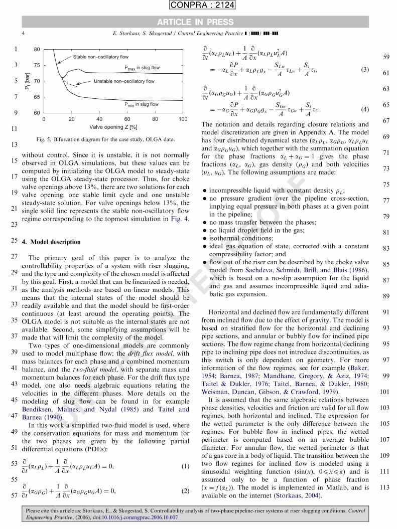
Fig. 6. Verification of tuned model for: (a) inlet pressure PI and (b)

pressure drop over choke valve DP.


ORRECT

5. Model tuning and verification

The model described above is similar, but significantlysimplified, compared to the one used in OLGA. For thepurpose of this work, the OLGA model is assumed toaccurately describe the (imaginary) real system, and datafrom the OLGA simulations are used to tune the model byfitting its parameters.

The level of tuning required for any mathematical modeldepends on the assumptions and simplifications made. Inthis case, it is assumed that the liquid density is constant. Infact, the density varies weakly with pressure, and a densitythat is representative for the current problem is needed.The same can be said about the equation of state; the idealgas law is used for simplicity, and some tuning on the gasmolecular weight and/or compressibility factor is needed asthese change throughout the system. Other importanttuning parameters are the proportionality constants in thefriction correlations and the average bubble diameter forbubbly flow in the riser (for determining wetted perimeterin inter-phase friction).

Still, even with all these tuning factors, obtaining a goodfit to the data for all valve openings is difficult. The systemis distributed, and the effect of each tuning parameter is notalways clear. The focus has been to achieve a goodqualitative fit to the data, as the main interest is to studythe general behavior of such a system. Also, for stabilizingcontrol, the main focus is studying the unstable stationaryoperating points (dashed line in Fig. 5) rather than thestable, undesired slug flow. Thus, the model is fitted mainlyto the stationary (unstable) operating line, and lessemphasis is put on the open-loop (uncontrolled) riserslugging behavior.

The tuning was done by manually adjusting the modelparameters using the bifurcation diagrams as tuning aids.The resulting fit is illustrated in Fig. 6, where the bold linesare the reference data (OLGA) and the thin lines arecomputed from the simple two-fluid model. The fit for thestable non-oscillatory flow regime (at low valve openings)is excellent, especially for the risertop pressure (Fig. 6(b)),whereas there are some deviations for the slug flow regime.Since the slug flow regime is undesirable, these deviationsare, as mentioned above, of less importance for controlpurposes.
C
103

105

107

109

111

113

UN6. Controllability analysis

The riser slugging case is interesting and challenging forcontrol because it turns out to contain many conflictingcontrollability limitations. The riser slugging phenomena isoscillatory, and it is found, as expected, that the unstable(RHP) poles pi are complex. The most serious challenge forstabilizing control (avoiding riser slugging), is that there,for some measurement alternatives, also are unstable(RHP) zeros z located close to the unstable (RHP) polespi. To motivate the controllability analysis, some of the



controllability problems will be illustrated by simulationsbefore some control theory is reviewed.

6.1. Introductory open-loop simulations

The main objective for anti-slug control is to stabilize thenon-oscillatory flow regime using the valve position Z as amanipulated variable. In theory, for linear systems, anymeasurement where the instability is observable may beused (Skogestad & Postlethwaite, 1996). However, inpractice input saturation (in magnitude or rate) or unstablezero dynamics (RHP-zeros) may prevent stabilization. Togain some insight into the dynamic properties, Fig. 7 showsthe simulated response to a step change in Z at t ¼ 0 forfour alternative measurements: inlet pressure (PI ), riserbase pressure (PRb), pressure drop over topside choke valve(DP) and volumetric flow out of the riser (Q). Theresponses are shown both for the simple two-fluid model(thin lines) and OLGA (bold lines).The valve position prior to the step is Z ¼ 10%, and a

2% step increase is applied, so this it at a point close toinstability. The simulations show that the step changeinduces oscillations, but because the step is made at a stable



skoge

Note

There seems to be some problems with Figure 6 - when I printed the file some solid lines became dotted, etc. Also, the solid (thick) lines are not as thick as they should be. I am therefore enclosing eps-files for Figure 6.

TED PROOF

ARTICLE IN PRESS

CONPRA : 2124

1

3

5

7

9

11

13

15

17

19

21

23

25

27

29

31

33

35

37

39

41

43

45

47

49

51

53

55

57

59

61

63

65

67

69

71

73

75

77

79

81

83

85

87

89

91

93

95

97

99

101

103

105

107

109

111

113

−1 0 1 2 3 4 570

71

72

73

74

0 20 40 60 80 100 12070

71

72

73

74

75

PI [B

ar]

Full Step response

0 20 40 60 80 100 12068

70

72

74

PR

b [B

ar]

−1 0 1 2 3 4 571

72

73

74

Initial response to step

0 20 40 60 80 100 120

3

4

5

6

DP

[B

ar]

−1 0 1 2 3 4 5

5

5.5

6

0 20 40 60 80 100 1200.015

0.02

0.025

Q [m

3/s

]

Time [min]

−1 0 1 2 3 4 50.015

0.02

0.025

Time [min]

Fig. 7. Open-loop responses with the simple two-fluid model (thin lines) and OLGA (bold lines) for a step in valve opening Z.


UNCORRECoperating point, these eventually die out. The oscillationsfor the OLGA simulation have a period of a 25min,corresponding to a frequency ofp ¼ 2p=ð25260 sÞ ¼ 0:004 s�1. The oscillations are a bitfaster for the two-fluid model, with a period of about17min corresponding to a frequency p ¼ 0:006 s�1.

For the three pressures, the main difference is for theinitial response shown at the right. The PRb, there is animmediate decreasing initial response and no problemswith stabilization are expected. For PI , there is an effectivedelay of about 10 s, which will make stabilization a bitmore difficult, but the time delay is probably not largeenough to cause major problems. For DP there is also aneffective delay of about 2min with the two-fluid model and4min with OLGA, caused by inverse response. Finally, forthe flow Q, the response is immediate, it is noted that thesteady-state gain is close to zero as Q eventually returns toits original value. This means that control of Q cannot beused to affect the steady-state behavior of the system. Thesmall steady-state gain for Q is easily explained because theinflow to the system is given, and the outflow must atsteady-state equal the inflow.



The inverse responses in the time domain for themeasurement y ¼ DP correspond to RHP-zeros in thetransfer function model (Skogestad & Postlethwaite, 1996).Also, the shape of the inverse response, with the initialresponse is in the ‘‘right’’ direction followed by a correctionin the ‘‘wrong’’ direction, indicate a complex pair of RHP-zeros. The transfer functions can be used to derive moreexact expressions for the deteriorating effect the RHP-zeroshave on control performance. Such expressions arediscussed next.

6.2. Controllability analysis: Theoretical background

6.2.1. Transfer functions

Consider a process y ¼ GðsÞuþ Gd ðsÞd and a feedbackcontroller u ¼ KðsÞðr� y� nÞ where d represents distur-bances and n the noise. The closed-loop response is

y ¼ Trþ SGdd � Tn, (5)

where S ¼ ðI þ GKÞ�1 and T ¼ GKðI þ GKÞ�1 ¼ I � S

are the sensitivity and complementary sensitivity function,respectively. The closed-loop input to the plant is



ARTICLE IN PRESS

CONPRA : 2124

1

3

5

7

9

11

13

15

17

19

21

23

25

27

29

31

33

35

37

39

41

43

45

47

49

51

53

55

57

59

61

63

65

67

69

71

73

75

77

79


u ¼ KSðr� Gdd � nÞ. (6)

In addition to the closed-loop transfer functions in (5) and(6), the transfer function SG gives the effect of inputdisturbances on the output y (set Gd ¼ G in (6)). Thetransfer functions S; T ; KS and SG can also be inter-preted as robustness to various kinds of uncertainty, wheresmall magnitudes for the closed-loop transfer functionsindicates good robustness properties. For example, S is thesensitivity toward inverse relative uncertainty, which is agood model of uncertainty in the pole locations (Skogestad& Postlethwaite, 1996).

Thus, by calculating the lower bounds for the closed-loop transfer functions S, T, KS, SG, KSGd and SGd ,information can be obtained regarding both achievableperformance and possible robustness problems. Thebounds on the H1 norm, kMk1 ¼ maxojMðjoÞj, whichis simply the peak value of the transfer function, will beconsidered. The bounds presented below are all indepen-dent of the controller K, and are thus a property of theprocess itself. The bounds are, however, dependent on asystematic and correct scaling of the process, which will beaddressed after the bounds has been introduced.

E

81

83

85

87

89

91

93

95

97

99

101

103

105

107

109

111

113

UNCORRECT

6.2.2. Lower bound on S and T

The lowest achievable peaks in sensitivity and comple-mentary functions, denoted MS;min and MT ;min, are closelyrelated to the distance between the unstable poles (pi) andzeros (zi). For SISO systems (Skogestad & Postlethwaite,1996) show that for any unstable (RHP) zero z:

kSk1XMS;min ¼YNp

i¼1

jzþ p̄ij

jz� pij. (7)

Note that the bound approaches infinity as z approaches pi.For systems with only one unstable zero, the bound

holds with equality. Chen (2000) shows that the bound in(7) also applies to kTk1, and generalizes the bound toapply for MIMO systems with any number of unstablepoles and zeros:

MS;min ¼MT ;min

¼

ffiffiffiffiffiffiffiffiffiffiffiffiffiffiffiffiffiffiffiffiffiffiffiffiffiffiffiffiffiffiffiffiffiffiffiffiffiffiffiffiffiffiffiffiffiffiffiffi1þ s̄2ðQ�1=2p QT

zpQ�1=2z Þ;q

ð8Þ

where the elements of the matrices Qz;Qp and Qzp are givenby

½Qz�ij ¼yH

z;iyz;j

zi þ z̄j

; ½Qp�ij ¼yH

p;iyp;j

p̄i þ pj

; ½Qzp�ij ¼yH

z;iyp;j

zi � pj

. (9)

The vectors yz;i and yp;i are the (unit) output directionvectors associated with the zero zi and pole pi, respectively.For SISO systems, these direction vectors all equal 1.

Time delays pose additional limitations. For example,Chen (2000) shows that the bound for kTk1 is increased bya factor jepyj for a single RHP-pole.



D PROOF

6.2.3. Lower bound on KS

The transfer function KS from measurement noise n toplant inputs u is at low frequencies closely related to theinverse of the process transfer function G. This can be seenby rewriting KS ¼ G�1T (using GKS ¼ T) and recallingthat with integral action, Tð0Þ ¼ I . Unstable plantsrequires control and a connection between KS and G�1 isalso found in the bound (Havre & Skogestad, 1997, 2001)

kKSk1XjGsðpÞ�1j, (10)

where Gs is the stable version of G with the RHP-poles of G

mirrored into the LHP. The bound is tight (with equality)for one real unstable pole p. For multiple and complexunstable poles pi (Glover, 1986), gives the tight bound

kKSk1X1=sH ðUðGÞÞ, (11)

where sHðUðGÞÞ is the smallest Hankel singular value ofthe antistable part of G.

6.2.4. Lower bound on SG and SGd

Chen (2000) reports that for any unstable zero z in G:

kSGk1XjGmsðzÞjYNp

i¼1

jzþ p̄ij

jz� pij, (12)

kSGdk1XjGd ;msðzÞjYNp

i¼1

jzþ p̄ij

jz� pij, (13)

where the subscript ms denotes the stable, minimum-phaseversion of the transfer function (both RHP-poles andRHP-zeros mirrored into the LHP). These bounds are onlytight for one unstable zero z, but since they are valid forany RHP-zero z, they can also be applied for systems withmultiple unstable zeros.

6.2.5. Lower bound on KSGd

The stable, minimum phase part Gd ;ms of Gd can beregarded as a weight on KS. Thus, for any unstable pole p

(Havre & Skogestad, 1997; Skogestad & Postlethwaite,2005):

kKSGdk1 ¼ jG�1s ðpÞj � jGd ;msðpÞj. (14)

The bound is only tight for one real unstable pole p. Formultiple and complex unstable poles pi, the followingbound is tight (Skogestad & Postlethwaite, 2005):

kKSGdk1X1=sH ðUðG�1d;msGÞÞ. (15)

6.2.6. Pole vectors

For a plant GðsÞ with state space realization (A;B;C;D),the output pole vector yp;i for a pole pi is defined by Havreand Skogestad (2003)

yp;i ¼ Cti, (16)

where ti is the right (normalized) eigenvector correspond-ing to pi (Ati ¼ piti). Havre and Skogestad (2003) finds,based on minimum input usage for stabilization, that themeasurement corresponding to the largest element in the



ARTICLE IN PRESS

CONPRA : 2124

1

3

5

7

9

11

13

15

17

19

21

23

25

27

29

31

33

35

37

39

41

43

45

47

49

51

53

55

57

59

61

63

65

67


output pole vectors should be used for stabilizing control.Correspondingly, for input selection, the input that has thelargest element in the input pole vector up;i ¼ BHqi, whereqi is the left eigenvector of A (qH

i A ¼ piqHi ), should be

selected. One limitation on the use of pole vectors is thatthe relationship between the magnitude of the input usageand the magnitude of the pole vectors elements only holdsfor plants with a single unstable pole p. In this case, there isa pair of complex conjugate unstable poles pi, but it will beshown that the pole vectors still give some informationabout measurement selection.

69

71

73

75

77

79

6.2.7. Low frequency performance

Disturbance rejection is not strictly required for stabiliz-ing control. However, to avoid the possible destabilizingeffect of nonlinearity, the system should not ‘‘drift’’ too faraway from its nominal operating point. To achieve low-frequency performance, the low-frequency gain must besufficiently large. Specifically, for perfect low-frequencydisturbance rejection, it is required that jGðjoÞjXjGdðjoÞjat frequencies o4od where jGd j41.

UNCORRECT

Table 2

Controllability data for the operating point Z ¼ 30%

Measurement Value Scaling Dy Smallest RHP-zerob Pole

PI [bar] 68.7 1 98.1c 0.30

PRb [bar] 68.2 1 1140c 0.31

DP [bar] 0.66 0.5 0:01� 0:01i 0.17

rT ½kg=m3� 427 50 0.015 9.27

W ½kg=s� 9 1 –c 0.63

Q ½m3=s� 0.0211 0.002 –c 0.59

Unstable poles at p ¼ 0:0045� 0:0108i.aWant these small.bWant these large.cRHP-zeros that are not important for the control problem.

Table 1

Controllability data for the operating point Z ¼ 17:5%

Measurement Value Scaling Dy Smallest RHP-zerob Pole

PI [bar] 70 1 99c 0.36

PRb [bar] 69.5 1 1155c 0.37

DP [bar] 1.92 1 0:01� 0:01i 0.21

rT ½kg=m3� 432 50 0.016 0.28

W ½kg=s� 9 1 –c 0.59

Q ½m3=s� 0.0208 0.002 –c 0.51

Unstable poles at p ¼ 0:0014� 0:0085i.aWant these small.bWant these large.cRHP-zeros that are not important for the control problem.



OF

6.3. Scaling

The models are scaled as outlined in Skogestad andPostlethwaite (1996), such that all signals in the systemshould be less than one in magnitude. This is both toinclude saturation effects and to be able to compare signalsof different magnitude.The outputs are scaled with respect to the maximum

allowed deviation given in Tables 1 and 2. These alloweddeviations are set such that they are of equal magnitudecompared to the expected variations, and should thus allowfor direct comparison between the different measurementwith respect to stabilizing control. Nonlinear effects causethe process gain to vary with valve opening, and in thiscase, the gain is smallest for large valve openings. There-fore, the input is scaled with the maximum allowed positivedeviation in valve opening. For example, with a nominalvalve opening of Z ¼ 30%, the input scaling is Du ¼ 70%.There are several different sources for uneven flow into

the riser in a pipeline-riser system. First, the feed into thepipeline itself can vary, caused by upstream events (e.gchanged production rate, routing of a different subset ofwells into the pipeline or unstable wells). Second, hydro-

ED PRO 81

83

85

87

89

91

93

95

97

99

101

103

105

107

109

111

113

Minimum bound on peaksa

vectorb jGð0Þjb jSj ¼ jT j jKSj jSGj jKSGd j jSGd j

3.3 1.0 0.30 0.0 0.35 0.005

3.3 1.0 0.28 0.0 0.33 0.004

6.1 4.3 0.62 16.8 0.97 5.5

0.27 2.6 0.64 14.6 0.55 4.7

0 1 0.17 0 0.32 0

0.33 1 0.17 0 0.32 0.002

Minimum bound on peaks a

vectorb jGð0Þjb jSj ¼ jT j jKSj jSGj jKSGd j jSGd j

18.9 1.0 0.03 0.0 0.06 0.0

19.0 1.0 0.03 0.0 0.06 0.0

17.6 1.6 0.04 17.1 0.08 0.95

1.5 1.4 0.03 28.6 0.07 1.60

0 1 0.02 0 0.06 0

1.8 1 0.02 0 0.06 0



ARTICLE IN PRESS

CONPRA : 2124

1

3

5

7

9

11

13

15

17

19

21

23

25

27

29

31

33

35

37

39

41

43

45

47

49

51

53

55

57

59

61

63

65

67

69

71

73

75

77

79

81

83

−2 0 2 4 6 8 10

x 10−3

−0.015

−0.01

−0.005

0

0.005

0.01

0.015

Re(p)

Imag(p

)

Z = 13%Z = 5% Z = 100%

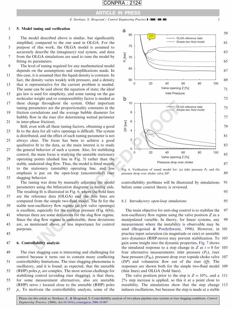
Fig. 9. Open-loop root-locus plot with valve opening Z as independent

parameter. Instability occurs at for ZX13%:


dynamic slugging, caused by the velocity differencebetween the liquid and the gas, can occur in the pipelineand give rise to uneven flow. Finally, terrain slugs, causedby accumulation of liquid in local low-points in thepipeline, can create small or medium-sized slugs in thepipeline. Flow variations into the pipeline are easilyrepresented as weighted feed disturbances. To include theeffect of hydrodynamic and terrain slugging in thecontrollability analysis without having to include thephysical effects that cause these phenomena in the model,it is assumed that the effect of hydrodynamic and terraininduced slugging can be approximated as sinusoidal feeddisturbances. Thus, it is assumed that the feed disturbancesW L and W G are frequency-dependent. The disturbanceweight

D ¼ 0:22p180

sþ 1� �

2p160

sþ 1� �

2p90

sþ 1� �

2p30

sþ 1� �2 , (17)

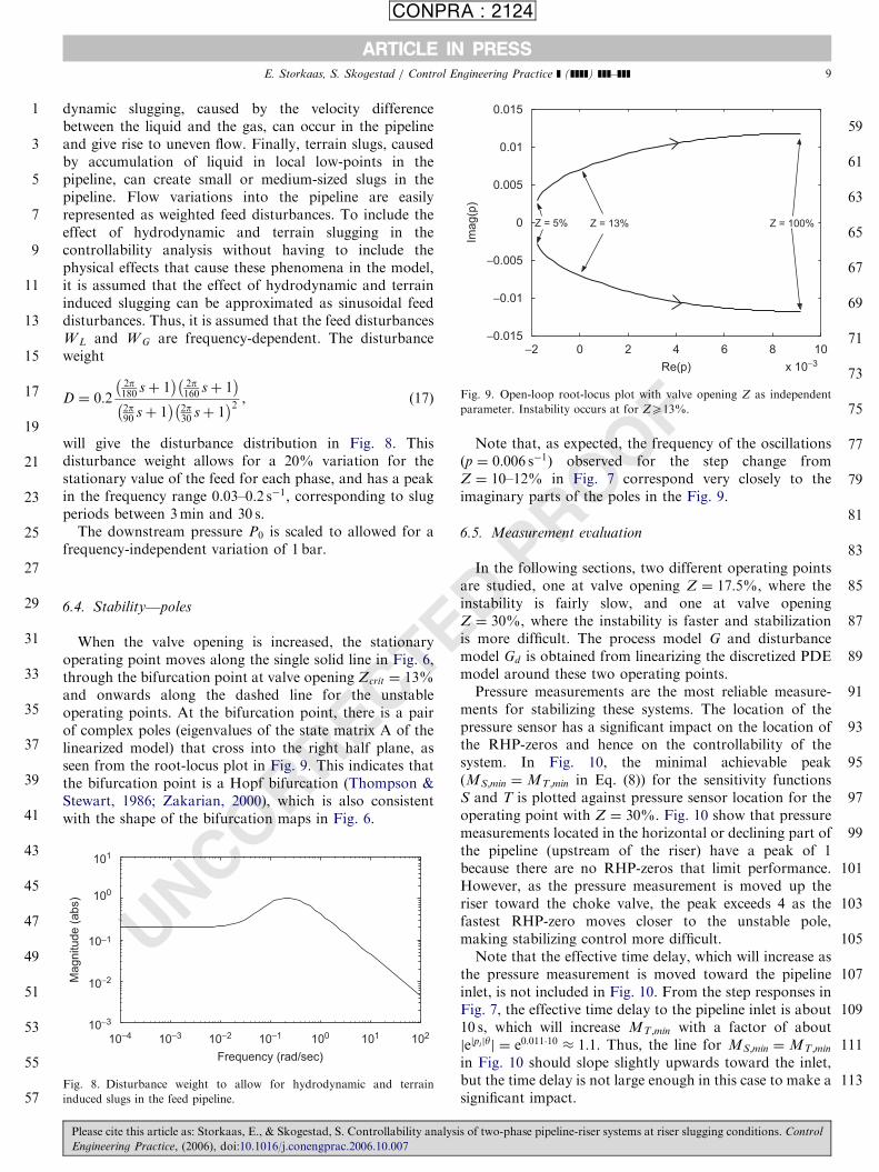
will give the disturbance distribution in Fig. 8. Thisdisturbance weight allows for a 20% variation for thestationary value of the feed for each phase, and has a peakin the frequency range 0.03–0:2 s�1, corresponding to slugperiods between 3min and 30 s.

The downstream pressure P0 is scaled to allowed for afrequency-independent variation of 1 bar.

E85

87

89

91

93

95

97
RRECT6.4. Stability—poles
When the valve opening is increased, the stationaryoperating point moves along the single solid line in Fig. 6,through the bifurcation point at valve opening Zcrit ¼ 13%and onwards along the dashed line for the unstableoperating points. At the bifurcation point, there is a pairof complex poles (eigenvalues of the state matrix A of thelinearized model) that cross into the right half plane, asseen from the root-locus plot in Fig. 9. This indicates thatthe bifurcation point is a Hopf bifurcation (Thompson &Stewart, 1986; Zakarian, 2000), which is also consistentwith the shape of the bifurcation maps in Fig. 6.

UNCO 99

101

103

105

107

109

111

113

10−4 10−3 10−2 10−1 100 101 10210−3

10−2

10−1

100

101

Magnitude (

abs)

Frequency (rad/sec)

Fig. 8. Disturbance weight to allow for hydrodynamic and terrain

induced slugs in the feed pipeline.



D PROOF

Note that, as expected, the frequency of the oscillationsðp ¼ 0:006 s�1Þ observed for the step change fromZ ¼ 10–12% in Fig. 7 correspond very closely to theimaginary parts of the poles in the Fig. 9.

6.5. Measurement evaluation

In the following sections, two different operating pointsare studied, one at valve opening Z ¼ 17:5%, where theinstability is fairly slow, and one at valve openingZ ¼ 30%, where the instability is faster and stabilizationis more difficult. The process model G and disturbancemodel Gd is obtained from linearizing the discretized PDEmodel around these two operating points.Pressure measurements are the most reliable measure-

ments for stabilizing these systems. The location of thepressure sensor has a significant impact on the location ofthe RHP-zeros and hence on the controllability of thesystem. In Fig. 10, the minimal achievable peak(MS;min ¼MT ;min in Eq. (8)) for the sensitivity functionsS and T is plotted against pressure sensor location for theoperating point with Z ¼ 30%. Fig. 10 show that pressuremeasurements located in the horizontal or declining part ofthe pipeline (upstream of the riser) have a peak of 1because there are no RHP-zeros that limit performance.However, as the pressure measurement is moved up theriser toward the choke valve, the peak exceeds 4 as thefastest RHP-zero moves closer to the unstable pole,making stabilizing control more difficult.Note that the effective time delay, which will increase as

the pressure measurement is moved toward the pipelineinlet, is not included in Fig. 10. From the step responses inFig. 7, the effective time delay to the pipeline inlet is about10 s, which will increase MT ;min with a factor of aboutjejpijyj ¼ e0:011�10 � 1:1. Thus, the line for MS;min ¼MT ;min

in Fig. 10 should slope slightly upwards toward the inlet,but the time delay is not large enough in this case to make asignificant impact.



ARTICLE IN PRESS

CONPRA : 2124

1

3

5

7

9

11

13

15

17

19

21

23

25

27

29

31

33

35

37

39

41

43

45

47

49

51

53

55

57

59

61

63

65

67

69

71

73

75

77

79

81

83

85

87

89

91

0 1000 2000 3000 4000 50001

1.5

2

2.5

3

3.5

4

4.5

Pressure sensor location (axial length form inlet [m])

MS

,min

= M

T,m

in

Bottom of riser

(PRb)

Choke Valve

(PT)

Inlet (PI)

Fig. 10. Minimum peaks on jSj and jT j (as given by the relative distance

between RHP-poles p and RHP-zeros z) as function of pressure sensor

location in pipeline.


CT

For practical reasons, the pressure sensors are usuallylocated at the pipeline inlet (PI ) and at the choke valve(PT ). For some pipelines, there is also a pressuremeasurement at the riser base (PRb). Since it is assumedthat the pressure P0 behind (downstream) the choke valveis constant, the pressure drop (DP ¼ PT � P0) over thechoke and the pressure in front of the choke (PT ) areequivalent. In addition to these pressure measurements, thedensity at the top of the riser (rT ), the mass flow throughthe choke (W) and the volumetric flow through the choke(Q) is included as measurement candidates for stabilizingcontrol.

Tables 1 and 2 summarizes the controllability results forthe two operating points. The tables give the nominal valuefor each measurement, scaling factor, the location of thesmallest unstable (RHP) zero, pole vector elements,nominal value, stationary gain as well as the lower boundson all the closed-loop transfer functions. The followingconclusions can be drawn from the tables:

93

95
�
97

99

102

P

E

RREIt is theoretically possible (with no model error) tostabilize the system with all the measurement candidatessince the input magnitude given by kKSk1 andkKSGdk1 are less than unity for all measurementcandidates.
�
101100

abs)
COUpstream pressure measurements (PI and PRb) are
particularly well suited for stabilizing control with alarge steady-state gain and all peaks small.

10310−2e (
�
105

107

10910−6

10−4Mag

nitu

d

GGd1 (WL)

Gd2 (WG)

Gd3 (P0)

UNIn practice, the pressure drop over the valve (DP) anddensity at the top of the riser (rT ) should not be used forstabilizing control because of the high peaks for jSj andjT j (about 4), indicating robustness problems. The peakfor jSGj is also large (about 20). The high peaks forthese transfer function are caused by RHP-zeros z closeto the RHP-poles p.
�
111

113

Frequency (rad/sec)

10−4 10−3 10−2 10−1 100 101 102

Fig. 11. Frequency dependent gain for y ¼ Q at operating point

Z ¼ 30%.

Flow measurements at the pipeline outlet (W or Q) canbe used for stabilizing control, also in practice.However, they both suffer from a close-to zerostationary gain (jGð0Þj ¼ 0 and 0:33, respectively), whichmeans that good low-frequency (steady-state) perfor-

lease cite this article as: Storkaas, E., & Skogestad, S. Controllability analysis of

ngineering Practice, (2006), doi:10.1016/j.conengprac.2006.10.007

mance is not possible. Note that the mass flow W haszero stationary gain because we assume that the feedrate is constant. For real systems, the feed rate ispressure dependent, and there would be a non-zero low-frequency gain, but it would probably still be too smallto allow for acceptable low-frequency performance.
� The pole vectors give the same general conclusions as
the closed-loop peaks, but since the link between polevectors and measurement selection only holds for plantswith a single unstable pole, the difference between thepole vector elements for the good and the bad controlvariables is not very large.

ED PROOF

6.6. Controllability analysis of flow control (y ¼ Q)

From Table 2, the potential problem with flow control(y ¼ Q) is a low steady-state gain. This is confirmed in Fig.11 the Bode magnitude plot of the linear scaled processmodel GðsÞ obtained at the operating point Z ¼ 30%,together with the models GdðsÞ for the three disturbances.The disturbance gain for the flow disturbances are high forlow frequencies and drops off sharply above abouto ¼ 0:2. Above o ¼ 0:2, flow disturbances are effectivelydampened through the pipeline. The downstream pressuredisturbance P0 does not pose a problem for control. Notethat the high-frequency gain for this disturbance isunrealistic, and stems from the fact that a constant scalingover all frequencies is used.Thus, if the volumetric flow ðy ¼ QÞ is chosen as the

primary controlled variable, the controller will not be ableto suppress low-frequency disturbances because the dis-turbance gain is higher that the process gain, jGd j4jGj.This may cause a disturbance to drive the operation into apoint where the controller no longer manages to stabilizethe process. This implies that this measurement is bestsuited to use in an inner loop in a cascade controller, ratherthan for independent stabilizing control.



E

ARTICLE IN PRESS

CONPRA : 2124

1

3

5

7

9

11

13

15

17

19

21

23

25

27

29

31

33

35

37

39

41

43

45

47

49

51

53

55

57

59

61

63

65

67

69

71

73

75

77

79

81

83

85

87

89

91

93

95


RECT

6.7. Controllability analysis of upstream pressure control

(y ¼ PI or y ¼ PRb)

From Tables 1 and 2, the upstream pressure measure-ments PI and PRb both seem to be very promisingcandidates for control. The Bode magnitude plot of thelinear scaled process model GðsÞ for the inlet pressurey ¼ PI , obtained at the operating point Z ¼ 30%, is shownin Fig. 12 together with the three disturbance models. Thecorresponding Bode plot for the riser base pressure(y ¼ PRb) is almost identical. The process gain is higherthat the disturbances, jGj4jGd j, for frequencies up toabout o ¼ 0:15. Above this frequency, the disturbance gainis lower than unity, and disturbance rejection is not strictlyneeded. However, the next section will show that the peakin the disturbance magnitude at o � 0:2 can, even if it isbelow 1, cause oscillatory flow out of the system andexcessive valve movement for the stabilized system.

The analysis has so far not considered the maindifference between the measurements PI and PRb, whichis the effective time delay due to pressure wave propagationin the pipeline. The simulations (both with OLGA and withthe simple two-fluid model) in Section 6 showed that thereare virtually no time delay through the riser to the riserbase measurement PRb, whereas the pressure wave takesabout 10 s to propagate back to the measurement PI . Thisimposes an upper bound on the closed-loop bandwidth ofthe system, as the crossover frequency oc needs to be lessthan the inverse of the time delay y, oco1=y. On the otherhand, the instability requires a bandwidth of approxi-mately oXjpj for complex unstable poles (Skogestad &Postlethwaite, 1996). With jpj � 0:01, this means that, forthis operating point, a closed-loop crossover frequency inthe range 0:015ooco0:1 is needed when using y ¼ PI . Foreven longer pipelines than the one studied in this example,the time delay may be too high for the inlet pressure to beused for stabilizing control.

Thus, the analysis shows that the riser base pressure PRb

and the inlet pressure PRb are good candidates for

UNCOR 97

99

101

103

105

107

109

111

113

10−4 10−3 10−2 10−1 100 101 102

10−6

10−4

10−2

100

102

Mag

nitu

de (

abs)

Frequency (rad/sec)

GGd1 (WL)

Gd2 (WG)

Gd3 (P0)

Fig. 12. Frequency dependent gain for y ¼ PI at operating point

Z ¼ 30%.



D PROOF

stabilizing control of these systems. With either of thesemeasurements, it should be possible to design a controllerthat stabilize the system with little input usage, is able toeffectively suppress (low-frequency) disturbances, and hasgood setpoint tracking properties. The main concern wouldbe to suppress flow disturbances in the medium-to-highfrequency range (flow disturbances with o � 0:2 s�1,corresponding to waves and/or hydrodynamic sluggingwith a period of about 30 s).

6.8. Additional remarks

So far, the main topic has been single input-single output(SISO) control, but from the above discussion, themeasurements have advantages in different frequencyranges. An upstream pressure measurement (PI or PRb)has excellent low-frequency properties, while a measure-ment of the flow through the choke valve (Q or W) hasgood high-frequency properties. Combining these twomeasurements in a cascade controller or a similar controlscheme that can utilize the benefits of both the measure-ment candidates would probably be a good way toapproach the problem. Such a scheme has indeed alreadybeen reported by Skofteland and Godhavn (2003) andGodhavn, Mehrdad, and Fuchs (2005). However, analysisof such systems is outside the scope of this work.It should also be mentioned that the operating point at

Z ¼ 30%, used in the above analysis, is a fairly aggressiveoperating point with relatively fast instability and lowprocess gain. If the same analysis were to be perform at themore conservative operating point (Z ¼ 17:5%), thecontrollability of the system would be significantlyimproved to a relatively minor cost in terms of pressuredrop.

7. Simulations

Since direct design of model-based optimal controllersare complicated due to the complexity of the model, simplePI-controllers are used to illustrate and confirm the resultsfrom the controllability analysis in Section 6. The simula-tions use the simple two-fluid model described in Section 4.One reason for not using the OLGA model is that it isdifficult with OLGA to impose the type of disturbancesthat is considered in this paper.

7.1. Stabilizing pressure control (y ¼ PI )

A simple feedback PI controller with controller gainKc ¼ �0:3 bar

�1 and integral time tI ¼ 500 s stabilizes thesystem and give a crossover frequency of oc ¼ 0:033 s�1 forthe operating point with Z ¼ 30%. The control system isillustrated in the left part of Fig. 13. However, nonlineareffects may make it difficult to stabilize the process directlyat this operating point starting from initial severe sluggingbehavior. A possible solution to this problem is to initiallystabilize the process at a less aggressive operating point and



ED PROOF

ARTICLE IN PRESS

CONPRA : 2124

1

3

5

7

9

11

13

15

17

19

21

23

25

27

29

31

33

35

37

39

41

43

45

47

49

51

53

55

57

59

61

63

65

67

69

71

73

75

77

79

81

83

85

87

89

91

93

95

97

99

101

103

105

107

109

111

113

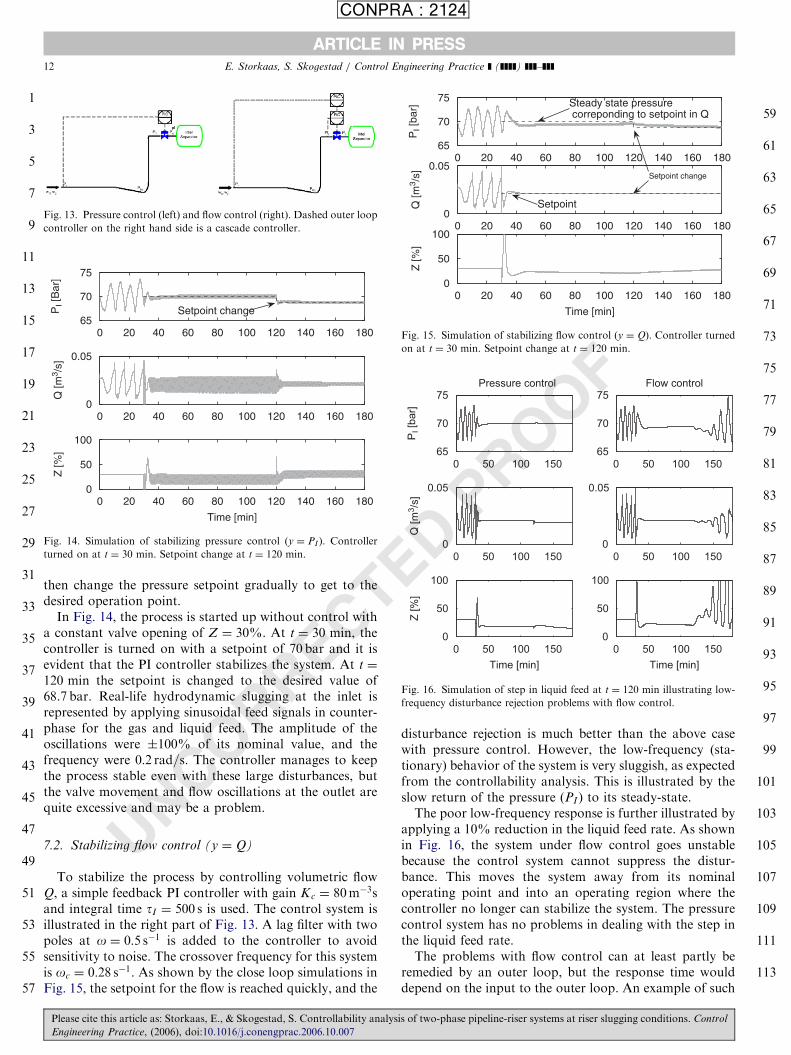
Fig. 13. Pressure control (left) and flow control (right). Dashed outer loop

controller on the right hand side is a cascade controller.

0 20 40 60 80 100 120 140 160 18065

70

75

PI [

Bar

]

0 20 40 60 80 100 120 140 160 1800

0.05

Q [m

3 /s]

0 20 40 60 80 100 120 140 160 1800

50

100

Time [min]

Z [%

]

Setpoint change

Fig. 14. Simulation of stabilizing pressure control (y ¼ PI ). Controller

turned on at t ¼ 30 min. Setpoint change at t ¼ 120 min.

0 20 40 60 80 100 120 140 160 18065

70

75

PI [

bar]

0 20 40 60 80 100 120 140 160 1800

0.05

Q [m

3 /s]

0 20 40 60 80 100 120 140 160 1800

50

100

Time [min]

Z [%

]

Setpoint

Steady state pressure correponding to setpoint in Q

Setpoint change

Fig. 15. Simulation of stabilizing flow control ðy ¼ QÞ. Controller turned

on at t ¼ 30 min. Setpoint change at t ¼ 120 min.

0 50 100 15065

70

75Flow control

0 50 100 1500

0.05

0 50 100 1500

50

100

Time [min]

0 50 100 15065

70

75

PI [b

ar]

Pressure control

0 50 100 1500

0.05

Q [m

3/s

]

0 50 100 1500

50

100

Time [min]

Z [%

]

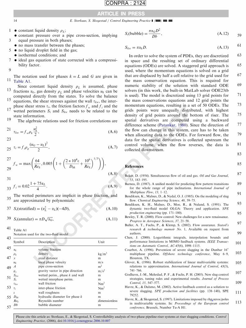
Fig. 16. Simulation of step in liquid feed at t ¼ 120 min illustrating low-

frequency disturbance rejection problems with flow control.


UNCORRECTthen change the pressure setpoint gradually to get to thedesired operation point.

In Fig. 14, the process is started up without control witha constant valve opening of Z ¼ 30%. At t ¼ 30 min, thecontroller is turned on with a setpoint of 70 bar and it isevident that the PI controller stabilizes the system. At t ¼

120 min the setpoint is changed to the desired value of68.7 bar. Real-life hydrodynamic slugging at the inlet isrepresented by applying sinusoidal feed signals in counter-phase for the gas and liquid feed. The amplitude of theoscillations were �100% of its nominal value, and thefrequency were 0:2 rad=s. The controller manages to keepthe process stable even with these large disturbances, butthe valve movement and flow oscillations at the outlet arequite excessive and may be a problem.

7.2. Stabilizing flow control (y ¼ Q)

To stabilize the process by controlling volumetric flowQ, a simple feedback PI controller with gain Kc ¼ 80m�3sand integral time tI ¼ 500 s is used. The control system isillustrated in the right part of Fig. 13. A lag filter with twopoles at o ¼ 0:5 s�1 is added to the controller to avoidsensitivity to noise. The crossover frequency for this systemis oc ¼ 0:28 s�1. As shown by the close loop simulations inFig. 15, the setpoint for the flow is reached quickly, and the



disturbance rejection is much better than the above casewith pressure control. However, the low-frequency (sta-tionary) behavior of the system is very sluggish, as expectedfrom the controllability analysis. This is illustrated by theslow return of the pressure (PI ) to its steady-state.The poor low-frequency response is further illustrated by

applying a 10% reduction in the liquid feed rate. As shownin Fig. 16, the system under flow control goes unstablebecause the control system cannot suppress the distur-bance. This moves the system away from its nominaloperating point and into an operating region where thecontroller no longer can stabilize the system. The pressurecontrol system has no problems in dealing with the step inthe liquid feed rate.The problems with flow control can at least partly be

remedied by an outer loop, but the response time woulddepend on the input to the outer loop. An example of such



E

ARTICLE IN PRESS

CONPRA : 2124

1

3

5

7

9

11

13

15

17

19

21

23

25

27

29

31

33

35

37

39

41

43

45

47

49

51

53

55

57

59

61

63

65

67

69

71

73

75

77

79

81

83

85

87

89

91

93

95

97

99

101

103

105

107

109

111

113

10−4 10−3 10−2 10−1 100 101 102

−1800

−1440

−1080

−720

−360

0

Phase (

deg)

10−10

100

Magnitude (

abs)

Fig. 17. Bode diagram for process model GðsÞ, y ¼ PI at Z ¼ 30%.


UNCORRECT

a control system is shown with the dashed outer loop onthe right side of Fig. 13.

8. Comments on model complexity

The PDE-model used in this paper is discretized in spaceto transform it into a system of ODE’s that is needed forconventional controllability analysis and controller design.The drawback of this model structure is that the modelorder (state dimension) of the resulting system of ODE’s ishigh (about 50 states), and the direct numerical optimiza-tion needed for design of (optimal) model based controllersgets complicated. Additionally, due to high model order,any controller based on a systematic design procedure,such as LQG control, will have a high number of states.This may be partly remedied by model reduction, but othersolutions may also be conceivable.

The Bode diagram for the linear process model obtainedaround the operating point Z ¼ 30% with y ¼ PI asmeasurement is given in Fig. 17. Both the phase and themagnitude are relatively smooth, and resemble a signifi-cantly simpler model than the one used in this work. Thisleads one to suspect that the underlying mechanics of thisprocess can be described using a greatly simplified model.This suspicion is further strengthened by physical argu-ments. The severe slugging is mainly a process driven bythe competing effects of the pressure in the upstream(horizontal/declining) part of the pipeline and the weight ofthe liquid in the riser. Since both pressure and gravity arebulk quantities, it should be possible to describe the processusing greatly simplified model based on bulk quantitiesrather than the distributed model used in this paper. Such asimplified model is presented in Storkaas (2005) andStorkaas, Skogestad, and Godhavn (2003).

9. Conclusions

In this paper, it is shown that riser slugging in pipelinescan be stabilized with simple control systems, but that thetype and location of the measured input to the controller is



D PROOF

critical. Of the possible candidates studied in this work,only an upstream (inlet or riser base) pressure measure-ment and a flow measurement at the outlet are viablecandidates for stabilizing control.Use of an upstream pressure measurement works well

for stabilization, but is less suited for suppressing high-frequency flow disturbances such as small hydrodynamicslugs that might be formed in the pipeline. It might also bea problem using the inlet pressure as a primary controlvariable for long pipelines due to the time delay associatedwith pressure wave propagation.Use of an outlet flow measurement is effective for

suppressing high-frequency flow disturbances. However,the low-frequency disturbance rejection and setpointtracking properties are poor, and this makes a stabilizingcontroller based on a topside flow measurement a viableoption only if it is used in combination with anothermeasurement (for example cascade or SIMO control).The analysis of the properties of this system reveals that

the underlying mechanics of the system probably can bedescribed by a simpler model than the PDE-based modelused in this work.

Acknowledgment

Thanks to Vidar Alstad, who participated in thedevelopment and implementation of the simplified two-fluid model used in this paper.

Appendix A. Modeling details

The PDE-based two-fluid model consist of massbalances (Eqs. (A.1) and (A.2)) and momentum balances(Eqs. (A.3) and (A.4)) for the liquid and gas phase. Thebalance equations combined with the summation equationfor the phase fraction (Eq. (A.5)) will give the four statesaLrL, aGrG, aLrLuL and aGrGuG:

qqtðaLrLÞ þ

1

A

qqxðaLrLuLAÞ ¼ 0, (A.1)

qqtðaGrGÞ þ

1

A

qqxðaGrGuGAÞ ¼ 0, (A.2)

qqtðaLrLuLÞ þ

1

A

qqxðaLrLu2

LAÞ

¼ �aLqP

qxþ aLrLgx �

SLw

AtLw þ

Si

Ati, ðA:3Þ

qqtðaGrGuGÞ þ

1

A

qqxðaGrGu2

GAÞ

¼ �aG

qP

qxþ aGrGgx �

SGw

AtGw þ

Si

Ati, ðA:4Þ

aL þ aG ¼ 1. (A.5)

The following assumptions form the basis for the model:

�

s of

one-dimensional flow;



ARTICLE IN PRESS

CONPRA : 2124

1

3

5

7

9

11

13

15

17

19

21

23

25

27

29

31

33

35

37

39

41

43

45

47

49

51

53

55

57


�

Ta

No

Sym

ak

rk

x

uk

A

gx

Skw

Si

tkw

ti

�Dhk

Rek

Db

P

E

constant liquid density rL;
59 � constant pressure over a pipe cross-section, implying
equal pressure in both phases;
61 � no mass transfer between the phases;
�
no liquid droplet field in the gas; 63 � isothermal conditions; and
�
65
67

69

71

73

75

77

79

81

83

85

87

89

91

93

95
RECT
ideal gas equation of state corrected with a compressi-bility factor.

The notation used for phases k ¼ L and G are given inTable A1.

Since constant liquid density rL is assumed, phasefractions ak, gas density rL and phase velocities uk can becomputed directly from the states. To solve the balanceequations, the shear stresses against the wall tkw, the inter-phase shear stress ti, the friction factors f w and f i and thewetted perimeters Si and Skw needs to be related to thestate information.

The algebraic relations used for friction correlations are

tkw ¼ f wrk

u2k

2, (A.6)

ti ¼ f irg

ðuG � uLÞ2

2, (A.7)

f w ¼ max64

Rek

; 0:005 1þ2 � 104�

Dhk

þ106

Rek

� �1=3 ! !

,

(A.8)

f i ¼ 0:021þ 75aL

4. (A.9)

The wetted perimeters are implicit in phase fraction, andare approximated by polynomials:

SiðstratifiedÞ ¼ ða2L � aLÞð�4DÞ, (A.10)

SiðannularÞ ¼ pDffiffiffiffiffiffiaG

p, (A.11)

UNCORble A1

tation used for the two-fluid model

bol Description Unit

volume fraction

density kg=m3

axial distance m

local phase velocity m/s

pipe cross-section m2

gravity vector in pipe direction m=s2

wetted perim., phase k and wall m

wetted interphase perim. m

wall friction Nm2

inter-phase friction Nm2

wall roughness m

hydraulic diameter for phase k m

Reynolds number dimensionless

bubble diameter m

lease cite this article as: Storkaas, E., & Skogestad, S. Controllability analys

ngineering Practice, (2006), doi:10.1016/j.conengprac.2006.10.007

ROOF

SiðbubbleÞ ¼paGD2

Db, (A.12)

Skw ¼ pakD. (A.13)

In order to solve the system of PDEs, they are discretizedin space and the resulting set of ordinary differentialequations (ODEs) are solved. A staggered grid approach isused, where the momentum equations is solved on a gridthat are displaced by half a cell relative to the grid used forthe mass conservation equation. This is required fornumeric stability of the solution with standard ODEsolvers (in this work, the built-in MatLab solver ODE23tbis used). The model is discretized using 13 grid points forthe mass conservations equations and 12 grid points themomentum equations, resulting in a set of 50 ODEs. Thegrids points were unequally distributed, with highestdensity of grid points around the bottom of riser. Thespatial derivatives are computed using a backwarddifference scheme (Patankar, 1980). Since the direction ofthe flow can change in this system, care has to be takenwhen allocating data to the ODEs. For forward flow, thedata for the spatial derivatives is collected upstream thecontrol volume, when the flow reverses, the data iscollected downstream.

97

99

101

103

105

107

109

111

113

ED PReferences

Baker, D. (1954). Simultaneous flow of oil and gas. Oil and Gas Journal,

53, 183–195.

Barnea, D. (1987). A unified model for predicting flow pattern transitions

for the whole range of pipe inclinations. International Journal of

Multiphase Flow, 13, 1–12.

Bendiksen, K., Malnes, D., & Nydal, O. J. (1985). On the modeling of slug

flow. Chemical Engineering Science, 40, 59–75.

Bendiksen, K. H., Malnes, D., Moe, R., & Nuland, S. (1991). The

dynamic two-fluid model OLGA: Theory and application. SPE

production engineering (pp. 171–180).

Bewley, T. R. (2000). Flow control: New challenges for a new renaissance.

Progress in Aerospace Sciences, 37, 21–58.

Buller, A. T., Fuchs, P., & Klemp, S. (2002). Flow assurance. Statoil’s

research & technology memoir No. 1, Available on request from

authors.

Chen, J. (2000). Logarithmic integrals, interpolation bounds and

performance limitations in MIMO feedback systems. IEEE Transac-

tions on Automatic Control, AC-45(6), 1098–1115.

Courbot, A. (1996). Prevention of severe slugging in the Dunbar 1600

multiphase pipeline. Offshore technology conference, May 6–9,

Houston, TX.

Glover, K. (1986). Robust stabilization of linear multivariable systems:

relations to approximation. International Journal of Control, 43(3),

741–766.

Godhavn, J.-M., Mehrdad, P. F., & Fuchs, P. H. (2005). New slug control

strategies, tuning rules and experimental results. Journal of Process

Control, 15, 547–577.

Havre, K., & Dalsmo, M. (2002). Active feedback control as a solution to

severe slugging. SPE production and facilities (pp. 138–148), SPE

79252.

Havre, K., & Skogestad, S. (1997). Limitations imposed by rhp zeros/poles

in multivariable systems. In: Proceedings of the European control

conference, Brussels, Number Tu-A H1.



skoge

Cross-Out

skoge

Replacement Text

RHP

ARTICLE IN PRESS

CONPRA : 2124

1

3

5

7

9

11

13

15

17

19

21

23

25

27

29

31

33

35

37

39

41

43

45

47

49

51

53

55

57

59


Havre, K., & Skogestad, S. (2001). Achievable performance of multi-

variable systems with unstable zeros and poles. International Journal of

Control, 48, 1131–1139.

Havre, K., & Skogestad, S. (2003). Selection of variables for stabilizing

control using pole vectors. IEEE Transaction on Automatic Control,

74(8), 1393–1398.

Havre, K., Stornes, K. O., & Stray, H. (2000). Taming slug flow in

pipelines. ABB Review, 4, 55–63.

Hedne, P., & Linga, H. (1990). Suppression of terrain slugging with

automatic and manual riser choking. Advances in Gas–Liquid Flows

(pp. 453–469).

Henriot, V., Courbot, A., Heintze, E., & Moyeux, L. (1999). Simulation of

process to control severe slugging: Application to the Dunbar pipeline.

SPE annual conference and exhibition, Houston, TX, SPE 56461.

Hollenberg, J. F., de Wolf, S., Meiring, & W. J. (1995). A method to

supress severe slugging in flow line riser systems. Proceedings of the

seventh international conference on multiphase technology conference.

Kovalev, K., Cruickshank, A., & Purvis, J. (2003). The slug suppression

system in operation. Offshore Europe 2003, Aberdeen, UK, SPE 84947.

Mandhane, J. M., Gregory, G. A., & Aziz, K. (1974). A flow pattern map

for gas-liquid flow in horizontal pipes. International Journal of

Multiphase Flow, 1, 537–553.

Patankar, S.V. (1980). Numerical heat transfer and fluid flow. Series in

computational methods in mechanics and thermal sciences. Washing-

ton, DC: Hemisphere Publishing Company.

Sachdeva, R., Schmidt, Z., Brill, J. P., & Blais, R. M. (1986). Two phase

flow through chokes, SPE 15657.

Sarica, C., & Tengesdal, J. Ø. (2000). A new technique to eliminating

severe slugging in pipeline/riser systems. SPE annual technical

conference and exhibition, Dallas, TX, SPE 63185.

Schmidt, Z., Brill, J. P., & Beggs, H. D. (1979). Choking can eliminate

severe slugging. Oil and Gas Journal, 230–238.

Skofteland, G., & Godhavn, J.-M. (2003). Suppression of slugs in

multiphase flow lines by active use of topside choke—field experience

UNCORRECTE



PROOF

and experimental results. In: Proceedings of multiphase ’03, San Remo,

Italy, 11–13 June 2003.

Skogestad, S., & Postlethwaite, I. (1996). Multivariable feedback control.

New York: Wiley.

Skogestad, S., & Postlethwaite, I. (2005). Multivariable feedback control

(2nd ed.). New York: Wiley.

Storkaas, E. (2004). Matlab source code for nonlinear PDE model.

Available at the homepage of Sigurd Skogestad: hwww.nt.ntnu.no/

users/skoge/software/i.

Storkaas, E. (2005). Stabilizing control and controllability: Control

solutions to avoid slug flow in pipeline-riser systems. Ph.D. thesis,

Norwegian University of Science and Technology.

Storkaas, E., Skogestad, S., & Godhavn, J.-M. (2003). A low-dimensional

model of severe slugging for controller design and analysis. In:

Proceedings of multiphase ’03, San Remo, Italy, 11–13 June 2003.

Taitel, Y. (1986). Stability of severe slugging. International Journal of

Multiphase Flow, 12(2), 203–217.

Taitel, Y., & Barnea, D. (1990). Two phase slug flow. Advances in Heat

Transfer, 20, 71–103.

Taitel, Y., Barnea, D., & Dukler, A. E. (1980). Modeling flow pattern

transitions for steady upward gas–liquid flow in vertical tubes. AIChE

Journal, 26, 345–354.

Taitel, Y., & Dukler, A. E. (1976). A model for predicting flow regime

transitions in horizontal and near horizontal gas–liquid flow. AIChE

Journal, 22, 47–55.

Thompson, J. M. T., & Stewart, H. B. (1986). Nonlinear dynamics and

chaos. New York: Wiley.

Weisman, J., Duncan, D., Gibson, J., & Crawford, T. (1979). Effect of

fluid properties and pipe diameter on two-phase flow patterns in

horizontal lines. International Journal of Multiphase Flow, 5, 437–460.

Zakarian, E. (2000). Analysis of two-phase flow instabilities in pipe-riser

systems. In: Proceedings of the ASME pressure vessels and piping

conference, Seattle.

D 61

63


http://www.nt.ntnu.no/users/skoge/software/

http://www.nt.ntnu.no/users/skoge/software/


W Þ Prod Type:FTP ED:SwarnaR model pp col fig :NILÞ PAGN ...

Documents

Transcript of W Þ Prod Type:FTP ED:SwarnaR model pp col fig :NILÞ PAGN ...