CONTRIBUTED RESEARCH ARTICLES 19

VSURF: An R Package for VariableSelection Using Random Forestsby Robin Genuer, Jean-Michel Poggi and Christine Tuleau-Malot

Abstract This paper describes the R package VSURF. Based on random forests, and for both regressionand classification problems, it returns two subsets of variables. The first is a subset of importantvariables including some redundancy which can be relevant for interpretation, and the second oneis a smaller subset corresponding to a model trying to avoid redundancy focusing more closely onthe prediction objective. The two-stage strategy is based on a preliminary ranking of the explanatoryvariables using the random forests permutation-based score of importance and proceeds using astepwise forward strategy for variable introduction. The two proposals can be obtained automaticallyusing data-driven default values, good enough to provide interesting results, but strategy can alsobe tuned by the user. The algorithm is illustrated on a simulated example and its applications to realdatasets are presented.

Introduction

Variable selection is a crucial issue in many applied classification and regression problems (seee.g. Hastie et al., 2001). It is of interest for statistical analysis as well as for modelisation or predictionpurposes to remove irrelevant variables, to select all important ones or to determine a sufficient subsetfor prediction. These main different objectives from a statistical learning perspective involve variableselection to simplify statistical problems, to help diagnosis and interpretation, and to speed up dataprocessing.

Genuer et al. (2010b) proposed a variable selection method based on random forests (Breiman,2001), and the aim of this paper is to describe the associated R package called VSURF and to illustrateits use on real datasets. The stable version of the package is available from the Comprehensive RArchive Network (CRAN) at http://CRAN.R-project.org/package=VSURF.1 In order to make thepaper self-contained, the description of the variable selection method is provided. A simulated toyexample and a classical real dataset are processed using VSURF. In addition, two real examples in ahigh-dimensional setting, not previously addressed by the authors, are used to illustrate the value ofthe strategy and the effectiveness of the R package.

Introduced by Breiman (2001), random forests (abbreviated RF in the sequel) are an attractivenonparametric statistical method to deal with these problems, since they require only mild conditionson the model supposed to have generated the observed data. Indeed, since RF are based on decisiontrees and use aggregation ideas, they allow us to consider in an elegant and versatile frameworkdifferent models and problems, namely regression, two-class and multiclass classifications.

Considering a learning set L = {(X1, Y1), . . . , (Xn, Yn)}, supposed to consist of independentobservations of the random vector (X, Y), we distinguish as usual the predictors (or explanatoryvariables), collected in the vector X = (X1, . . . , Xp) where X ∈ Rp, from the explained variableY ∈ Y where Y is either a class label for classification problems or a numerical response for regressionones. Let us recall that a classifier t is a mapping t : Rp → Y while the regression function naturallycorresponds to the function s when we suppose that Y = s(X) + ε with E[ε|X] = 0. Then randomforests provide estimators of either the Bayes classifier, which minimizes the classification errorP(Y 6= t(X)), or the regression function.

The CART (Classification and Regression Trees) method defined by Breiman et al. (1984) is awell-known way to design optimal single binary decision trees. It proceeds by performing first agrowing step and then a pruning one. The principle of random forests is to aggregate many binarydecision trees coming from two random perturbation mechanisms: the use of bootstrap samples ofL instead of L and the random choice of a subset of explanatory variables at each node instead ofall of them. There are two main differences with respect to CART trees: first, in the growing step, ateach node, a fixed number of input variables are randomly chosen and the best split is calculated onlyamong them and, second, no pruning step is performed so all the trees of the forest are maximal trees.The RF algorithm is a very popular machine learning algorithm and appears to be powerful in a lotof different applications, see for example Verikas et al. (2011) and Boulesteix et al. (2012) for recentsurveys.

Several implementations of these methods are available. Focusing on R packages we must mentionrpart (Therneau et al., 2015) for CART, randomForest (Liaw and Wiener, 2002) for RF, party (Hothorn

1The current development version of the package is also available at https://github.com/robingenuer/VSURF.

The R Journal Vol. 7/2, December 2015 ISSN 2073-4859

CONTRIBUTED RESEARCH ARTICLES 20

et al., 2006) for CART and RF (through the function cforest) and ipred (Peters et al., 2002) for bagging(Breiman, 1996), a closely related method cited here for the sake of completeness. In this paper, we usethe randomForest procedure, which is based on the initial contribution of Breiman and Cutler (2004).We will concentrate on the prediction performance of RF focusing on the out-of-bag (OOB) error (seeBreiman, 2001) and on the quantification of the variable importance (VI in the sequel) which are keyingredients for our variable selection strategy. For a general discussion about variable importance, seeAzen and Budescu (2003). In the random forests framework, one of the most widely used scores ofimportance of a given variable is the increase in mean of the error of a tree (mean square error (MSE)for regression and misclassification rate for classification) in the forest when the observed values ofthis variable are randomly permuted in the OOB samples (see Archer and Kimes, 2008).

Strobl et al. (2007) showed that VI scores are biased towards correlated variables, and Stroblet al. (2008) proposed an alternative permutation scheme as a solution, which, however, increases thecomputation cost. This seems to be especially critical for high-dimensional problems with stronglycorrelated predictors. Nevertheless, our previous experiments (Genuer et al., 2010b) on variableselection and, more recently, the theoretical study of Gregorutti et al. (2013) show that, in somesituations, the VI scores are biased towards uncorrelated variables. Additional theoretical results andexperiments are needed to more deeply understand these phenomenons, but this is out of the scope ofthe paper.

A lot of variable selection procedures are based on the combination of variable importance forranking and model estimation to generate, evaluate and compare a family of models, i.e., in particularin the family of “wrapper” methods (Kohavi and John, 1997; Guyon and Elisseeff, 2003) which includethe prediction performance in the score calculation, for which a lot of methods can be cited. We chooseto highlight one of them which is widely used and close to our procedure. Díaz-Uriarte and AlvarezDe Andres (2006) propose a strategy based on recursive elimination of variables. At the beginning,they compute RF variable importance and then, at each step, eliminate iteratively the 20% of thevariables having the smallest importance and build a new forest with the remaining variables. Thefinal set of variables is selected by minimizing over the obtained forests, the OOB error rate definedby:

errOOB =

{1n Card {i ∈ {1, . . . , n} | yi 6= yi} in the classification framework1n ∑i∈{1,...,n} (yi − yi)

2 in the regression framework

where yi is the aggregation of the predicted values by trees t for which (xi, yi) belongs to the associatedOOB sample (data not included in the bootstrap sample used to construct t). The proportion ofvariables to eliminate is an arbitrary parameter of their method and does not depend on the data. Letus remark that we propose an heuristic strategy which does not depend on specific model hypotheses,but which is based on data-driven thresholds to take decisions.

This topic of variable selection still continues to be of interest. Indeed recently Hapfelmeier andUlm (2012) propose a new variable selection approach using random forests and, more generally,Cadenas et al. (2013) describe and compare different approaches in a survey paper.

Some packages are available to cope with variable selection problems. Let us cite, for classificationproblems the R package Boruta, described in Kursa and Rudnicki (2010), which aims at findingall relevant variables using a random forest classification algorithm which iteratively removes thevariables using a statistical test. The R package varSelRF, described in Díaz-Uriarte (2007), implementsthe previously described method for selecting very small sets of genes in the context of classification.The R package ofw (Lê Cao and Chabrier, 2008), also dedicated to the context of classification, selectsrelevant variables based on the application of supervised multiclass classifiers such as CART orsupport vector machines. The R package spikeSlabGAM implements Bayesian variable selectionvia regularized estimation in additive mixed models (Scheipl, 2011). Dedicated to the biomarkeridentification in the life sciences, the R package BioMark implements two meta-statistics for variableselection (Wehrens et al., 2012): the first sets a data-dependent selection threshold for significance,which is useful when two groups are compared, and the second, more general one, uses repeatedsubsampling and selects the model coefficients remaining consistently important.

The paper is organized as follows. After this introduction, we present the general variable selectionstrategy. We then describe how to use package VSURF on a simple simulated dataset. Finally, weexamine three real-life examples to illustrate the method in action in high-dimensional situations aswell as in a standard one.

The R Journal Vol. 7/2, December 2015 ISSN 2073-4859

CONTRIBUTED RESEARCH ARTICLES 21

The strategy

Objectives

In Genuer et al. (2010b) we distinguished two variable selection objectives referred to as interpretationand prediction.

Even if this distinction can be a little bit confusing since we use for both objectives the samecriterion related to prediction performance, the idea is the following. The first objective, calledinterpretation, is to find important variables highly related to the response variable, even with someredundancy, possibly high. The second one, namely prediction, is to find a smaller number of variableswith very low redundancy and sufficient for a good enough prediction of the response variable. Theterminology used here can be misunderstood since usually for interpretation, one usually looks forparsimony but in many situations one may often want to identify all predictor variables associatedwith the response to interpret correctly the relation. We thank one anonymous reviewer for raisingthis issue and we detail an example in the next paragraph to clarify the difference.

A typical situation illustrates the distinction between the two kinds of variable selection. Let usconsider a high-dimensional (n � p) classification problem for which the predictor variables areassociated to a pixel in an image or a voxel in a 3D-image as in fMRI brain activity classificationproblems (see e.g. Genuer et al., 2010a). In such situations, it is supposed that a lot of variables areuseless and that there exist unknown groups of highly correlated predictors corresponding to brainregions involved in the response to a given stimulation. The two distinct objectives about variableselection can be of interest. Finding all the important variables highly related to the response variableis useful for interpretation, since it corresponds to the determination of entire regions in the brain or afull parcel in an image. By contrast, finding a small number of variables sufficient for good predictionallows to get the most discriminant variables within the previously highlighted regions. For a moreformal approach to this distinction, see also the interesting paper Nilsson et al. (2007).

Principle

The principle of the two-steps algorithm is the following. First, we rank the variables according toa variable importance measure and the unimportant ones are eliminated. Second, we provide twodifferent subsets obtained either by considering a collection of nested RF models and selecting thevariables of the most accurate one, or by introducing sequentially the sorted variables.

Since the quantification of the variable importance is crucial for our procedure, let us recall thedefinition of RF variable importance. For each tree t of the forest, consider the associated OOBt sample(data not included in the bootstrap sample used to construct t). Denote by errOOBt the error (MSE forregression and misclassification rate for classification) of a single tree t on this OOBt sample. Now,

randomly permute the values of X j in OOBt to get a perturbed sample denoted by OOBtj

and compute

errOOBtj, the error of predictor t on the perturbed sample. Variable importance of X j is then equal to:

VI(X j) =1

ntree ∑t

(errOOBt

j− errOOBt

),

where the sum is over all trees t of the RF and ntree denotes the number of trees of the RF. Notice thatwe use this definition of importance and not the normalized one. Indeed, instead of considering (asmentioned in Breiman and Cutler, 2004) that the raw VI are independent replicates, normalizing themand assuming normality of these scores, we prefer a fully data-driven solution. This is a key point ofour strategy: we prefer to estimate directly the variability of importance across repetitions of forestsinstead of using normality when ntree is sufficiently large, which is only valid under some specificconditions. Those conditions are difficult to check since their validity depends heavily on tuningparameters and problem peculiarities, so data-driven normalization prevents some misspecifiedasymptotic behavior.

Another useful argument, which provides the rationale for this kind of variable selection procedurebased on a classical stepwise method combined with the use of a VI measure, is that a variable notincluded in the underlying true model has a null “theoretical” importance. In a recent paper Gregoruttiet al. (2013) theoretically state that, in the case of additive models, irrelevant variables have null“theoretical” VI. A similar result for the mean decrease impurity index (not used in this paper) hasbeen proven by Louppe et al. (2013).

The R Journal Vol. 7/2, December 2015 ISSN 2073-4859

CONTRIBUTED RESEARCH ARTICLES 22

Detailed strategy

Let us now describe more precisely our two-steps procedure. Note that each RF is typically built usingntree = 2000 trees.

• Step 1. Preliminary elimination and ranking:

– Rank the variables by sorting the VI (averaged over typically 50 RF runs) in descendingorder.

– Eliminate the variables of small importance (let m denote the number of remaining vari-ables).More precisely, starting from this order, consider the ordered sequence of the correspond-ing standard deviations (sd) of VI and use it to estimate a threshold value for VI. Sincevariability of VI is larger for true variables compared to useless ones, the threshold value isgiven by an estimation of the VI standard deviation of the useless variables. This thresholdis set to the minimum prediction value given by a CART model where the Y are the sd ofthe VI and the X are the ranks.Then only the variables with an averaged VI exceeding this threshold are retained.

• Step 2. Variable selection:

– For interpretation: construct the nested collection of RF models involving the k first vari-ables, for k = 1 to m and select the variables involved in the model leading to the smallestOOB error. This leads to consider m′ variables.More precisely, we compute OOB error rates of RF (averaged typically over 25 runs) of thenested models starting from the one with only the most important variable, and endingwith the one including all important variables previously kept. Ideally, the variables ofthe model leading to the smallest OOB error are selected. In fact, in order to deal withinstability, we use a classical trick: we select the smallest model with an OOB error lessthan the minimal OOB error augmented by its standard deviation (based on the same 25runs).

– For prediction: starting with the ordered variables retained for interpretation, construct anascending sequence of RF models, by invoking and testing the variables in a stepwise way.The variables of the last model are selected.More precisely, the sequential variable introduction is based on the following test: avariable is added only if the error decrease is larger than a threshold. The idea is that theOOB error decrease must be significantly greater than the average variation obtained byadding noisy variables. The threshold is set to the mean of the absolute values of the firstorder differentiated OOB errors between the model with m′ variables and the one with mvariables:

1m−m′

m−1

∑j=m′| errOOB(j + 1)− errOOB(j), | (1)

where errOOB(j) is the OOB error of the RF built using the j most important variables.

Comments

In addition to the detailed strategy, let us give some additional comments. Regarding the first step ofour procedure, our previous simulation study in Genuer et al. (2010b) shows that both VI level andvariability are larger for relevant variables.

We assume that the stabilized ranking performed in the first step of our procedure will not changeafter the elimination step.

The use of CART to find the threshold is of course not strictly necessary and can be replaced bymany other strategies but it is interesting in our case because the idea is typically to find a constant ona large interval. Since CART fits a piece-wise constant function, this desired constant is the thresholdfor VI and is defined as the minimum prediction value given by a CART model fitting the curve ofVI standard deviations. It is obtained automatically by the CART strategy whereas the user needs toselect some window parameter if, for example, a simple smoothing method is used.

Note that the threshold value is based on VI standard deviations while the effective thresholdingis performed on the VI mean. In general, this rule is conservative and leads to keep more variablesthan necessary, postponing to the next step a more parsimonious choice.

In addition, we note that several implementation choices have been made: randomForest for RFfitting and VI calculation (repeated 50 times to quantify variability) and rpart for estimating the VI

The R Journal Vol. 7/2, December 2015 ISSN 2073-4859

CONTRIBUTED RESEARCH ARTICLES 23

variability level associated with irrelevant variables leading to a convenient threshold value. Of courseother choices would be possible, for example, using the function cforest of the package party toimplement the same scheme of variable selection.

The next section describes the use of the package VSURF together with a complete illustration ofthe strategy which is not supported by specific model hypotheses but based on data-driven thresholdsto take decisions.

But before entering in this description, let us emphasize that the objects of interest here are thesubsets of important variables and not precisely the corresponding models. Thus OOB errors from thefigures (or from the fitted objects) cannot be used or reported as the prediction error estimation of thefinal model because this would need a proper cross-validation scheme.

Using the package VSURF

From data to final results

We illustrate the use of the VSURF package on a simple simulated moderately high-dimensionaldataset (n = 100 < p = 200) called toys data, introduced by Weston et al. (2003). It comes from anequiprobable two-class problem, Y ∈ {−1, 1}, with 6 influential variables and with the others beingnoise variables. Let us define the simulation model by giving the conditional distribution of the Xi forY = y:

• For the six first variables: with probability 0.7, Xi ∼ N (yi, 1) for i = 1, 2, 3 and Xi ∼ N (0, 1)for i = 4, 5, 6; with probability 0.3, Xi ∼ N (0, 1) for i = 1, 2, 3 and Xi ∼ N (y(i− 3), 1) fori = 4, 5, 6.

• The remaining variables are noise: Xi ∼ N (0, 1) for i = 7, . . . , p.

The variables obtained in the simulation are standardized before further analysis.

First, we load the VSURF package and the toys data (and fix the random number generation seedfor reproducibility):

> library("VSURF")> data("toys")> set.seed(3101318)

The standard way to use the VSURF package is to use the VSURF function. This function executesthe complete procedure, and is just a wrapper for the three intermediate functions VSURF_thres,VSURF_interp and VSURF_pred which are described in the next section. Typical use of the VSURFfunction is as follows:

> toys.vsurf <- VSURF(x = toys$x, y = toys$y, mtry = 100)

The only mandatory inputs are x, an object containing input variables, and y, the output variable.

In this example, we also choose a specific value for mtry (default is p/3 for classification andregression problems in VSURF), which only affects RF runs in the first step of the procedure. In addition,we stress that the default value for ntree is 2000 in VSURF. Those values were considered as welladapted for VI calculations (see Genuer et al., 2010b, Section 2.2) and these two arguments are passedto the randomForest function (we kept the same name for consistency).

The function outputs a list containing all results.

> names(toys.vsurf)

[1] "varselect.thres" "varselect.interp" "varselect.pred"[4] "nums.varselect" "imp.varselect.thres" "min.thres"[7] "imp.mean.dec" "imp.mean.dec.ind" "imp.sd.dec"[10] "mean.perf" "pred.pruned.tree" "err.interp"[13] "sd.min" "err.pred" "mean.jump"[16] "nmin" "nsd" "nmj"[19] "overall.time" "comput.times" "ncores"[22] "clusterType" "call"

The most important objects are varselect.thres, varselect.interp and varselect.pred, whichcontain the set of variables selected after the thresholding, interpretation and prediction step respec-tively.

The summary method gives a short summary of the results: numbers of selected variables andcomputation times.

The R Journal Vol. 7/2, December 2015 ISSN 2073-4859

CONTRIBUTED RESEARCH ARTICLES 24

0 50 100 150 200

0.00

0.05

0.10

0.15

variables

VI m

ean

0 50 100 150 200

0.00

000.

0015

0.00

30

variables

VI s

tand

ard

devi

atio

n0 5 10 15 20 25 30 35

0.05

0.10

0.15

nested models

OO

B e

rror

1.0 1.5 2.0 2.5 3.0

0.02

0.06

0.10

predictive models

OO

B e

rror

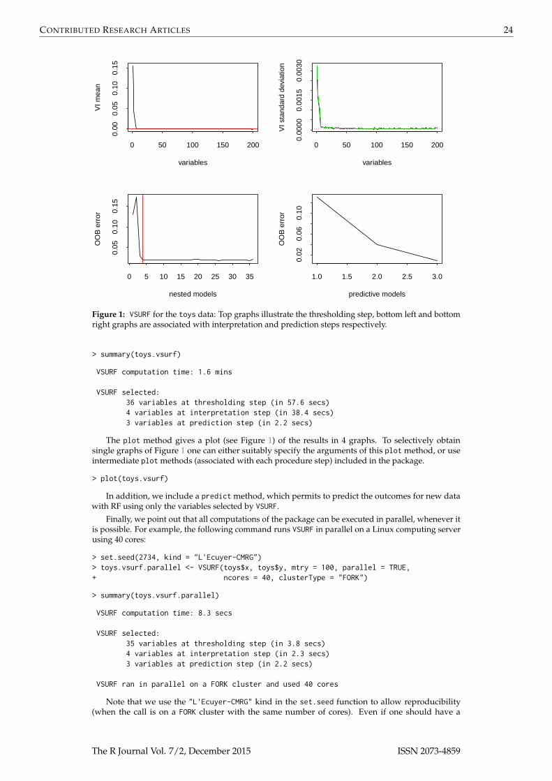
Figure 1: VSURF for the toys data: Top graphs illustrate the thresholding step, bottom left and bottomright graphs are associated with interpretation and prediction steps respectively.

> summary(toys.vsurf)

VSURF computation time: 1.6 mins

VSURF selected:36 variables at thresholding step (in 57.6 secs)4 variables at interpretation step (in 38.4 secs)3 variables at prediction step (in 2.2 secs)

The plot method gives a plot (see Figure 1) of the results in 4 graphs. To selectively obtainsingle graphs of Figure 1 one can either suitably specify the arguments of this plot method, or useintermediate plot methods (associated with each procedure step) included in the package.

> plot(toys.vsurf)

In addition, we include a predict method, which permits to predict the outcomes for new datawith RF using only the variables selected by VSURF.

Finally, we point out that all computations of the package can be executed in parallel, whenever itis possible. For example, the following command runs VSURF in parallel on a Linux computing serverusing 40 cores:

> set.seed(2734, kind = "L'Ecuyer-CMRG")> toys.vsurf.parallel <- VSURF(toys$x, toys$y, mtry = 100, parallel = TRUE,+ ncores = 40, clusterType = "FORK")

> summary(toys.vsurf.parallel)

VSURF computation time: 8.3 secs

VSURF selected:35 variables at thresholding step (in 3.8 secs)4 variables at interpretation step (in 2.3 secs)3 variables at prediction step (in 2.2 secs)

VSURF ran in parallel on a FORK cluster and used 40 cores

Note that we use the "L'Ecuyer-CMRG" kind in the set.seed function to allow reproducibility(when the call is on a FORK cluster with the same number of cores). Even if one should have a

The R Journal Vol. 7/2, December 2015 ISSN 2073-4859

CONTRIBUTED RESEARCH ARTICLES 25

0 50 100 150 200

0.00

000

0.00

010

0.00

020

variables

VI s

tand

ard

devi

atio

n

Figure 2: Zoom of the top right graph of Figure 1.

computing server with 40 cores to benefit from this execution time reduction, the resulting ‘VSURF’object from this call will be the same on a computer with fewer cores available. Parallel calls of VSURFwill be used to deal with the two high-dimensional datasets at the end of the paper.

How to get intermediate results

Let us now detail the main stages of the procedure together with the results obtained on the toys data.Note that unless explicitly stated otherwise, all graphs refer to Figure 1.

• Step 1.

– Variable ranking.The result of variable ranking is drawn on the top left graph. True variables are significantlymore important than the noisy ones.

– Variable elimination.Starting from this order, the plot of the corresponding standard deviations of VI is usedto estimate a threshold value for VI. This threshold (figured by the dotted horizontal redline in Figure 2, which is a zoom of the top right graph of Figure 1) is set to the minimumprediction value given by a CART model fitting this curve (see the green piece-wiseconstant function on the same graph).Then only the variables with an averaged VI exceeding this level (i.e. above the horizontalred line in the top left graph of Figures 1) are retained.The computation of the 50 forests, the ranking and elimination steps are obtained with theVSURF_thres function:

> set.seed(3101318)> toys.thres <- VSURF_thres(toys$x, toys$y, mtry = 100)

The VSURF_thres function outputs a list containing all results of this step. The mainoutputs are: varselect.thres which contains the indices of variables selected by this step,imp.mean.dec and imp.sd.dec which hold the VI mean and standard deviation (the orderaccording to decreasing VI mean can be found in imp.mean.dec.ind).

> toys.thres$varselect.thres

[1] 3 2 6 5 1 4 184 37 138 159 81 17 180 131 52 191[17] 96 192 165 94 198 25 21 109 64 12 29 188 107 157 70 46[33] 54 143 186 111

Finally, Figure 2 can be obtained with the following command:

> plot(toys.vsurf, step = "thres", imp.mean = FALSE, ylim = c(0, 2e-4))

We can see in the plot of the VI standard deviations (top right graph of Figure 1) that thetrue variables’ standard deviations are large compared to those of the noisy variables,which are close to zero.

The R Journal Vol. 7/2, December 2015 ISSN 2073-4859

CONTRIBUTED RESEARCH ARTICLES 26

• Step 2.

– Variable selection procedure for interpretation.We use VSURF_interp for this step. Note that we have to specify the indices of variablesselected at the previous step. So we set argument vars to toys.thres$varselect.thres:

> toys.interp <- VSURF_interp(toys$x, toys$y,+ vars = toys.thres$varselect.thres)

The list resulting from the VSURF_interp function mainly contains varselect.interp: thevariables selected by this step, and err.interp: OOB error rates of RF nested models.

> toys.interp$varselect.interp

[1] 3 2 6 5

In the bottom left graph, we see that the error decreases quickly. It reaches its (almost)minimum when the first four true variables are included in the model (see the vertical redline) and then it remains nearly constant. The selected model contains variables V3, V2,V6, V5, which are four of the six true variables, while the actual minimum is reached for35 variables.Note that, to ensure quality of OOB error estimations (e.g. Genuer et al., 2008, Section 2)along embedded RF models, the mtry parameter of the randomForest function is here setto its default value if k (the number of variables involved in the current RF model) is notgreater than n, while it is set to k/3 otherwise.

– Variable selection procedure for prediction.We use the VSURF_pred function for this step. We need to specify the error rates andthe variables selected in the interpretation step in the err.interp and varselect.interparguments:

> toys.pred <- VSURF_pred(toys$x, toys$y,+ err.interp = toys.interp$err.interp,+ varselect.interp = toys.interp$varselect.interp)

The main outputs of the VSURF_pred function are the variables selected by this final step,varselect.pred, and the OOB error rates of RF models, err.pred.

> toys.pred$varselect.pred

[1] 3 6 5

For the toys data, the final model for prediction purpose involves only variables V3, V6,V5 (see the bottom right graph). The threshold is set to the mean of the absolute values ofthe first order differentiated OOB errors between the model with m′ = 4 variables and theone with m = 36 variables.

Finally, we mention that VSURF_thres and VSURF_interp can be executed in parallel with the samesyntax as VSURF (setting parallel = TRUE), while VSURF_pred cannot be parallelized.

Tuning the different steps of the procedure

We provide two additional functions for tuning the thresholding and interpretation steps withouthaving to rerun all computations.

• First, a tune method which, applied to the result of VSURF_thres, can be used to tune thethresholding step. We can use the nmin parameter (which has default value 1) in order to set thethreshold to the minimum prediction value given by the CART model times nmin.

> toys.thres.tuned <- tune(toys.thres, nmin = 3)> toys.thres.tuned$varselect.thres

[1] 3 2 6 5 1 4 184 37 138 159 81 17 180 131 52 191

We get 16 selected variables instead of 36 previously.

• Secondly, a tune method which, applied to the result of VSURF_interp, is of the same kind andallows to tune the interpretation step. If we now want to be more restrictive in our selectionin the interpretation step, we can select the smallest model with an OOB error less than theminimal OOB error augmented by its empirical standard deviation times nsd (with nsd ≥ 1).

> toys.interp.tuned <- tune(toys.interp, nsd = 5)> toys.interp.tuned$varselect.interp

The R Journal Vol. 7/2, December 2015 ISSN 2073-4859

CONTRIBUTED RESEARCH ARTICLES 27

[1] 3 2 6

We get 3 selected variables instead of 4 previously.

We did not write a tuning method for the prediction step because it is a recursive step and needs torecompute the sequence. Hence, to adjust the parameter for this step, we have to rerun the VSURF_predfunction with a different value of nmj (which has default value 1). This multiplicative constant allowsto modulate the threshold defined in (1).

For example, increasing the value of nmj leads to selection of fewer variables:

> toys.pred.tuned <- VSURF_pred(toys$x, toys$y, err.interp = toys.interp$err.interp,+ varselect.interp = toys.interp$varselect.interp,+ nmj = 70)> toys.pred.tuned$varselect.pred

[1] 3 6

Remark

Thanks to one of the three anonymous reviewers, we would like to give a warning followinga remark made by Svetnik et al. (2004). Indeed, this work considers a situation where there is nolink between X and Y and for which they use OOB errors in a recursive strategy, different but nottoo far from our procedure, to select variables. Their results show that this kind of strategy can beseriously biased and can overfit the data. To illustrate explicitly this phenomenon, let us start with theoriginal dataset toys for which our procedure performs quite well (see the paper Genuer et al., 2010b,containing an extensive study of the operating characteristics of the algorithm including no overfittingin presence of many additional dummy variables). Then, modify it by scrambling the Y values thusremoving the link between X and Y. Applying VSURF on this modified dataset leads to an OOB errorrate, in the interpretation step, starting from 50% (which is correct) and exhibiting a minimum for 10variables corresponding to 37%. So, in this situation for which there is no optimal solution and thedesirable behavior is to find a constant OOB error rate along the sequence, the procedure still providesa solution. So, the conclusion is that even when there is no link between X and Y the procedure canhighlight a set of variables.

Of course, using an external 5-fold cross-validation of our entire procedure leads to the correctestimate of 51% error rate for both interpretation and prediction steps and the correct conclusion: thereis nothing to find in the data. Alternatively, if we simulate a second sample coming from the samesimulation model and use it only to rank the variables, the interpretation step exhibits an OOB errorrate curve oscillating around 50%, which leads to the correct conclusion.

Three illustrative examples

In this section we apply the proposed procedure on three real-life examples: two high-dimensionaldatasets (associated with a regression problem and a classification one respectively) and, before that, astandard one to illustrate the versatility of the procedure.

Let us mention that the VSURF stability is a natural issue to investigate (see e.g. Meinshausen andBühlmann, 2010) and is considered in Genuer et al. (2010b) Sections 3 and 4.

Ozone data

The Ozone dataset consists of n = 366 observations for 12 independent variables and 1 dependentvariable. These variables are numbered as in the R package mlbench (Leisch and Dimitriadou, 2010):1 – Month, 2 – Day of month, 3 – Day of week, 5 – Pressure height, 6 – Wind speed, 7 – Humidity,8 – Temperature (Sandburg), 9 – Temperature (El Monte), 10 – Inversion base height, 11 – Pressuregradient, 12 – Inversion base temperature, 13 – Visibility, for independent variables and 4 – Dailymaximum one-hour-average ozone, for the dependent variable.

What makes the use of this dataset interesting, is that it has already been extensively studied andthat even though it is a real one, it is possible to a priori know which variables are expected to beimportant. Moreover, this dataset, which is not a high-dimensional one, includes some missing data,allowing us to give an example of how to handle such data using VSURF.

To begin, we load the data:

> data("Ozone", package = "mlbench")> set.seed(221921186)

The R Journal Vol. 7/2, December 2015 ISSN 2073-4859

CONTRIBUTED RESEARCH ARTICLES 28

05

1015

20

variables

VI m

ean

V9 V8 V12 V1 V11 V5 V10 V7 V13 V6 V3 V2

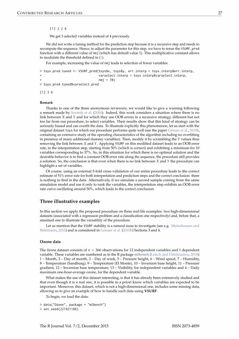
Figure 3: Sorted VI mean associated with the 12 explanatory variables of the Ozone data, with variablenames on the x-axis.

Then, we apply the complete procedure via VSURF. Note that the following formula-type call isnecessary to handle missing values (as in randomForest).

> vozone <- VSURF(V4 ~ ., data = Ozone, na.action = na.omit)> summary(vozone)

VSURF computation time: 1.7 mins

VSURF selected:9 variables at thresholding step (in 1.1 mins)5 variables at interpretation step (in 26.3 secs)5 variables at prediction step (in 12.4 secs)

In the first step, we look at the variable importance associated with each of the explanatory variables.

> plot(vozone, step = "thres", imp.sd = FALSE, var.names = TRUE)

In Figure 3, and as noticed in previous studies, three very sensible groups of variables can bediscerned ranging from the most to the least important. The first group contains the two temperatures(8 and 9), the inversion base temperature (12) known to be the best ozone predictors, and the month(1), which is an important predictor since ozone concentration exhibits an heavy seasonal component.The second group of clearly less important meteorological variables consists of: pressure height (5),humidity (7), inversion base height (10), pressure gradient (11) and visibility (13). Finally the lastgroup contains three unimportant variables: day of month (2), day of week (3) of course and moresurprisingly wind speed (6). This last fact is classical: wind enters in the model only when ozonepollution arises, otherwise wind and pollution are weakly correlated (see for example Chèze et al.,2003, who highlight this phenomenon using partial estimators).

Let us now examine the results of the selection procedures. To reflect the order used in thedefinition of the variables, we reorder the output variables of the procedure.

> number <- c(1:3, 5:13)> number[vozone$varselect.thres]

[1] 9 8 12 1 11 5 10 7 13

After the first elimination step, the 3 variables of negative importance (variables 6, 3 and 2) areeliminated, as expected.

> number[vozone$varselect.interp]

[1] 9 8 12 1 11

Then the interpretation procedure leads to select the model with 5 variables, which contains all ofthe most important variables.

The R Journal Vol. 7/2, December 2015 ISSN 2073-4859

CONTRIBUTED RESEARCH ARTICLES 29

> number[vozone$varselect.pred]

[1] 9 8 12 1 11

With the default settings, the prediction step does not remove any additional variable.

Remark

Even though the comparison with other variable selection strategies is out of the scope of the paper,one of the three anonymous reviewers has kindly compared the results of the VSURF package withthe results of the R package Boruta, described in Kursa and Rudnicki (2010), on the two datasets toysand Ozone.

Let us recall that this module directly aims at selecting all-relevant features. Hence the comparisonwith the interpretation set delivered by VSURF is of interest. In the toys dataset, the number of trulyrelevant variables is 6. VSURF finds 4 out of 6 variables in the interpretation stage while Borutafinds all six truly relevant variables and one more false positive variable. In the case of the Ozonedata set VSURF finds 5 variables in the interpretation stage, while Boruta finds 9. So, this seems toconfirm that the heuristic proposed by VSURF is prediction oriented (the price to pay is a risk offalse negatives) and suggests that the strategy proposed by Boruta is more accurate to recover weakredundant correlations between predictors and decision variable (the price to pay seems to be a risk offalse positives).

In fact our strategy assumes more or less that there are unnecessary variables in the set of allavailable variables initially, which is not really the case in the Ozone dataset. However, it is the case inthe following two high-dimensional examples.

Toxicity data

This second dataset is also a regression framework, however, unlike before, this case is a high-dimensional problem. The liver.toxicity dataset, available in the R package mixOmics (Lê Caoet al., 2015), is a real dataset from a study by Heinloth et al. (2004). In this study, 4 male rats ofthe inbred strain Fisher 344 were exposed to different doses of acetaminophen (non toxic dose (50or 150 mg/kg), moderate toxic dose (1500 mg/kg), severe toxic dose (2000 mg/kg)) in a controlledexperiment. Necropsies were performed at different hours after exposure (6, 18, 24 and 48 hours)and the mRNA from the liver was extracted. In the original study, 10 clinical chemistry variablescontaining markers for the liver injury were measured. Those variables are numerical variables sincethey measure the serum enzymes level. For our analysis, the dataset extracted from this study contains:

• a data frame, called gene, with 64 rows representing the subjects and 3116 columns repre-senting explanatory variables which are the gene expression levels after normalization andpreprocessing due to Bushel et al. (2007),

• a vector, called clinic, with 64 rows and 1 column, one of the 10 clinical variables for the same64 subjects: more precisely, the variable named ALB.g.dL., which corresponds to the albuminlevel and which is the one considered in González et al. (2012).

As in previous studies (Gidskehaug et al., 2007; Lê Cao et al., 2008), our aim is, using VSURF, topredict our clinical variable by the genes.

First, we load the data as follows:

> data("liver.toxicity", package = "mixOmics")> clinic <- liver.toxicity$clinic$ALB.g.dL.> set.seed(7162013, "L'Ecuyer-CMRG")

Now we apply our procedure and analyze the results.

> vtoxicity <- VSURF(liver.toxicity$gene, clinic, parallel = TRUE, ncores = 40,+ clusterType = "FORK")

> summary(vtoxicity)

VSURF computation time: 5.9 mins

VSURF selected:550 variables at thresholding step (in 1.1 mins)5 variables at interpretation step (in 4.8 mins)5 variables at prediction step (in 3.4 secs)

VSURF ran in parallel on a FORK cluster and used 40 cores

The R Journal Vol. 7/2, December 2015 ISSN 2073-4859

CONTRIBUTED RESEARCH ARTICLES 30

0 500 1500 2500

0.00

000.

0010

variables

VI m

ean

0 500 1500 2500

0.00

000

0.00

015

variables

VI s

tand

ard

devi

atio

n0 100 200 300 400 500

0.03

00.

040

0.05

0

nested models

OO

B e

rror

1 2 3 4 5

0.03

00.

040

0.05

0predictive models

OO

B e

rror

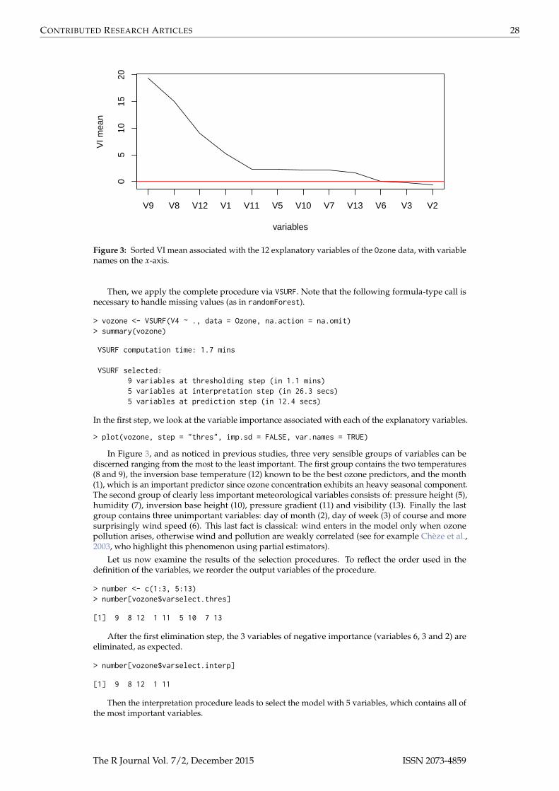
Figure 4: VSURF for the toxicity data.

We notice that after the elimination step, only 550 variables remain, thus the number of variableshas been reduced by a factor of six. This ratio is not surprising since we know that there exists extremeredundancy in the gene expression data together with a lot of irrelevant variables.

> plot(vtoxicity)

By considering the top left graph of Figure 4, it seems quite obvious to keep just a few variables.Indeed, the procedure leads to 5 variables, after both interpretation and prediction steps. Even if thenumbers of selected variables are very small, they are not surprisingly low if we refer to the studyin González et al. (2012), where 12 variables were selected. It would be noted that, in general, ourmethod failed to deliver all the variables related to the response variable in the case of numerousstrongly correlated predictors. In addition, we do not select the same genes but our set of selectedvariables and the one in González et al. (2012) exhibit strong correlations.

Even if the results are quite similar, an advantage of using VSURF is that this procedure does notinvolve tuning parameters unlike the procedure developed in González et al. (2012). This difference isthe main reason for the gap in computation time: several minutes with 40 cores for VSURF compared toseveral minutes with 1 core for González et al. (2012).

SRBCT data

The dataset we consider here will allow us to apply our procedure in a classification framework. Thereal classification dataset is a small version of the small round blue cell tumors of childhood data andcontains the expression measure of genes measured on 63 samples. This set is composed of:

• a data frame, called gene, of size 63 × 2308 which contains the 2308 gene expressions;

• a response factor of length 63, called class, indicating the class of each sample (4 classes intotal).

These data, presented in details in Khan et al. (2001), available in the R package mixOmics, havebeen widely studied but in most cases only 200 genes were considered and data have been transformedto reduce the problem to a regression problem (see e.g. Lê Cao and Chabrier, 2008). As in Díaz-Uriarteand Alvarez De Andres (2006), we consider the 2308 genes and we deal directly with the classificationproblem, using VSURF.

> data("srbct", package = "mixOmics")> set.seed(10131419, "L'Ecuyer-CMRG")

The R Journal Vol. 7/2, December 2015 ISSN 2073-4859

CONTRIBUTED RESEARCH ARTICLES 31

> vSRBCT <- VSURF(srbct$gene, srbct$class, parallel = TRUE, ncores = 40,+ clusterType = "FORK")

> summary(vSRBCT)

VSURF computation time: 3.6 mins

VSURF selected:676 variables at thresholding step (in 22.6 secs)25 variables at interpretation step (in 3 mins)13 variables at prediction step (in 13.6 secs)

VSURF ran in parallel on a FORK cluster and used 40 cores

On this dataset, the procedure leads to 25 and 13 selected variables after the interpretation andprediction step respectively, and the selected variable sets are stable.

We can compare these results with those obtained in Díaz-Uriarte and Alvarez De Andres (2006)where the authors select 22 genes on the original dataset and their number of selected variables isquite stable.

To get an idea of the performance of our procedure on the dataset, we perform an error rateestimation using an external 5-fold cross-validation scheme (meaning that we apply VSURF on eachfold of the cross-validation). We obtain the following error rates2 for interpretation and prediction setsrespectively:

interp pred0.01587302 0.07936508

The comparison with error rates evaluated using 200 bootstrap samples in Díaz-Uriarte andAlvarez De Andres (2006) suggests that our selections are reasonable.

Acknowledgements

We thank the editor and the three anonymous referees for their thorough comments and suggestionswhich really helped to improve the clarity of the paper.

Bibliography

K. J. Archer and R. V. Kimes. Empirical characterization of random forest variable importance measures.Computational Statistics & Data Analysis, 52(4):2249–2260, 2008. [p20]

R. Azen and D. V. Budescu. The dominance analysis approach for comparing predictors in multipleregression. Psychological Methods, 8(2):129–148, 2003. [p20]

A.-L. Boulesteix, S. Janitza, J. Kruppa, and I. R. König. Overview of random forest methodology andpractical guidance with emphasis on computational biology and bioinformatics. Wiley Interdisci-plinary Reviews: Data Mining and Knowledge Discovery, 2(6):493–507, 2012. [p19]

L. Breiman. Bagging predictors. Machine Learning, 24(2):123–140, 1996. [p20]

L. Breiman. Random forests. Machine Learning, 45(1):5–32, 2001. [p19, 20]

L. Breiman and A. Cutler. Random forest manual. 2004. URL http://www.stat.berkeley.edu/~breiman/RandomForests/cc_manual.htm. [p20, 21]

L. Breiman, J. Friedman, R. Olshen, and C. Stone. Classification and Regression Trees. Chapman & Hall,New York, 1984. [p19]

P. Bushel, R. Wolfinger, and G. Gibson. Simultaneous clustering of gene expression data with clinicalchemistry and pathological evaluations reveals phenotypic prototypes. BMC Systems Biology, 1(1):15, 2007. [p29]

J. M. Cadenas, M. Carmen Garrido, and R. Martínez. Feature subset selection filter-wrapper based onlow quality data. Expert Systems with Applications, 40(16):6241–6252, 2013. [p20]

2The script is available at https://github.com/robingenuer/VSURF/blob/master/Example/srbct_cv.R

The R Journal Vol. 7/2, December 2015 ISSN 2073-4859

CONTRIBUTED RESEARCH ARTICLES 32

N. Chèze, J.-M. Poggi, and B. Portier. Partial and recombined estimators for nonlinear additive models.Statistical Inference for Stochastic Processes, 6(2):155–197, 2003. [p28]

R. Díaz-Uriarte. GeneSrF and varSelRF: A web-based tool and R package for gene selection andclassification using random forest. BMC Bioinformatics, 8(1):328, 2007. [p20]

R. Díaz-Uriarte and S. Alvarez De Andres. Gene selection and classification of microarray data usingrandom forest. BMC Bioinformatics, 7(1):3, 2006. [p20, 30, 31]

R. Genuer, J.-M. Poggi, and C. Tuleau. Random forests: Some methodological insights. 2008.arXiv:0811.3619. [p26]

R. Genuer, V. Michel, E. Eger, and B. Thirion. Random forests based feature selection for decoding fMRIdata. In Proceedings of COMPSTAT’2010 – 19th International Conference on Computational Statistics,pages 1071–1078, 2010a. [p21]

R. Genuer, J.-M. Poggi, and C. Tuleau-Malot. Variable selection using random forests. PatternRecognition Letters, 31(14):2225–2236, 2010b. [p19, 20, 21, 22, 23, 27]

L. Gidskehaug, E. Anderssen, A. Flatberg, and B. K. Alsberg. A framework for significance analysis ofgene expression data using dimension reduction methods. BMC Bioinformatics, 8(1):346, 2007. [p29]

I. González, K.-A. Lê Cao, M. J. Davis, and S. Déjean. Visualising associations between paired ’omics’data sets. BioData Mining, 5(1):1–23, 2012. [p29, 30]

B. Gregorutti, B. Michel, and P. Saint-Pierre. Correlation and variable importance in random forests.2013. arXiv:1310.5726. [p20, 21]

I. Guyon and A. Elisseeff. An introduction to variable and feature selection. Journal of Machine LearningResearch, 3:1157–1182, 2003. [p20]

A. Hapfelmeier and K. Ulm. A new variable selection approach using random forests. ComputationalStatistics & Data Analysis, 60:50–69, 2012. [p20]

T. Hastie, R. Tibshirani, and J. H. Friedman. The Elements of Statistical Learning. Springer-Verlag, NewYork, 2001. [p19]

A. N. Heinloth, R. D. Irwin, G. A. Boorman, P. Nettesheim, R. D. Fannin, S. O. Sieber, M. L. Snell, C. J.Tucker, L. Li, G. S. Travlos, G. Vansant, P. E. Blackshear, R. W. Tennant, M. L. Cunningham, andR. S. Paules. Gene expression profiling of rat livers reveals indicators of potential adverse effects.Toxicological Sciences, 80(1):193–202, 2004. [p29]

T. Hothorn, K. Hornik, and A. Zeileis. Unbiased recursive partitioning: A conditional inferenceframework. Journal of Computational and Graphical Statistics, 15(3):651–674, 2006. [p19]

J. Khan, J. S. Wei, M. Ringner, L. H. Saal, M. Ladanyi, F. Westermann, F. Berthold, M. Schwab, C. R.Antonescu, C. Peterson, and P. S. Meltzer. Classification and diagnostic prediction of cancers usinggene expression profiling and artificial neural networks. Nature Medicine, 7(6):673–679, 2001. [p30]

R. Kohavi and G. H. John. Wrappers for feature subset selection. Artificial Intelligence, 97(1):273–324,1997. [p20]

M. B. Kursa and W. R. Rudnicki. Feature selection with the Boruta package. Journal of StatisticalSoftware, 36(11):1–13, 2010. [p20, 29]

K.-A. Lê Cao and P. Chabrier. ofw: An R package to select continuous variables for multiclassclassification with a stochastic wrapper method. Journal of Statistical Software, 28(9):1–16, 2008. [p20,30]

K.-A. Lê Cao, D. Rossouw, C. Robert-Granié, and P. Besse. A sparse PLS for variable selection whenintegrating omics data. Statistical Applications in Genetics and Molecular Biology, 7(1), 2008. [p29]

K.-A. Lê Cao, I. Gonzalez, and S. Dejean. mixOmics: Omics Data Integration Project, 2015. URLhttps://CRAN.R-project.org/package=mixOmics. R package version 5.0-4, with key contributionsfrom F. Rohart and B. Gautier and contributions from P. Monget, J. Coquery, F. Yao and B. Liquet.[p29]

F. Leisch and E. Dimitriadou. mlbench: Machine Learning Benchmark Problems, 2010. URL https://CRAN.R-project.org/package=mlbench. R package version 2.1-1. [p27]

The R Journal Vol. 7/2, December 2015 ISSN 2073-4859

CONTRIBUTED RESEARCH ARTICLES 33

A. Liaw and M. Wiener. Classification and regression by randomForest. R News, 2(3):18–22, 2002. [p19]

G. Louppe, L. Wehenkel, A. Sutera, and P. Geurts. Understanding variable importances in forests ofrandomized trees. In Advances in Neural Information Processing Systems, pages 431–439, 2013. [p21]

N. Meinshausen and P. Bühlmann. Stability selection. Journal of the Royal Statistical Society B, 72(4):417–473, 2010. [p27]

R. Nilsson, J. M. Peña, J. Björkegren, and J. Tegnér. Consistent feature selection for pattern recognitionin polynomial time. Journal of Machine Learning Research, 8:589–612, 2007. [p21]

A. Peters, T. Hothorn, and B. Lausen. ipred: Improved predictors. R News, 2(2):33–36, 2002. [p20]

F. Scheipl. spikeSlabGAM: Bayesian variable selection, model choice and regularization for generalizedadditive mixed models in R. Journal of Statistical Software, 43(14):1–24, 2011. [p20]

C. Strobl, A.-L. Boulesteix, A. Zeileis, and T. Hothorn. Bias in random forest variable importancemeasures: Illustrations, sources and a solution. BMC Bioinformatics, 8(1):25, 2007. [p20]

C. Strobl, A.-L. Boulesteix, T. Kneib, T. Augustin, and A. Zeileis. Conditional variable importance forrandom forests. BMC Bioinformatics, 9(1):307, 2008. [p20]

V. Svetnik, A. Liaw, C. Tong, and T. Wang. Application of Breiman’s random forest to modelingstructure-activity relationships of pharmaceutical molecules. In Multiple Classifier Systems, pages334–343. Springer, 2004. [p27]

T. Therneau, B. Atkinson, and B. Ripley. rpart: Recursive Partitioning and Regression Trees, 2015. URLhttps://CRAN.R-project.org/package=rpart. R package version 4.1-9. [p19]

A. Verikas, A. Gelzinis, and M. Bacauskiene. Mining data with random forests: A survey and resultsof new tests. Pattern Recognition, 44(2):330–349, 2011. [p19]

H. R. Wehrens, M. Johan, and P. Franceschi. Meta-statistics for variable selection: The R packageBioMark. Journal of Statistical Software, 51(10):1–18, 2012. [p20]

J. Weston, A. Elisseeff, B. Schölkopf, and M. Tipping. Use of the zero norm with linear models andkernel methods. Journal of Machine Learning Research, 3:1439–1461, 2003. [p23]

Robin GenuerUniversity of BordeauxISPED, Centre INSERM U-897-Epidemiologie-Biostatistique33000 Bordeaux, FranceandINRIA Bordeaux Sud Ouest, SISTM team33400 Talence, FranceRobin.Genuer@isped.u-bordeaux2.fr

Jean-Michel PoggiUniversity of OrsayLab. Mathematicsbat 42591405 Orsay, FranceJean-Michel.Poggi@math.u-psud.fr

Christine Tuleau-MalotUniversity of Nice Sophia AntipolisCNRS, LJAD, UMR 735106100 Nice, FranceMalot@unice.fr

The R Journal Vol. 7/2, December 2015 ISSN 2073-4859