Vsh or Element to Mineral Methods: Take your Best Shot. · Robert V. Everett Petrophysics, Inc....
26
GeoConvention 2018 1 Vsh or Element to Mineral Methods: Take your Best Shot. Robert V. Everett Robert V. Everett Petrophysics, Inc. Summary Today’s most exact log interpretation relies on an Element-Mineral method, correcting resistivity in shale using Cation Exchange Capacity. Most commercial programs rely on the more traditional Vsh method, correcting for non-permeable zones with a volume of shale. The EM method, has been relevant for thirty years, thanks to ongoing refinements with new tool measurements. When do we choose the EM method? Also pointed out, is a need for a Dielectric measurement (Ref. 14), since incorrect formation water resistivity (Rw) is the bane of all interpretation programs. Considerations 1) Element-Mineral derived CEC is an upgrade to Vsh, because more information is available; For example, sandclass from elements, grain density from elements, Rw from SP [because CEC corrects the Ro for clay conductivity]. 2) When elements are not recorded, they can be predicted from offset wells to make full use of the element to mineral method. Predicted data has caveats: one assumes the depositional environments are similar. This means the elements associated with the minerals are similar. For example, in reducing environments like the Montney, sulphur is present and is associated with pyrite. Hence, sulphur and some iron is bound in the pyrite and the program would calculate pyrite. Whereas, the association of sulphur in a non-reducing carbonate environment is more likely anhydrite. Hence, one should not predict elements from a shale gas environment and use the predicted element in a lithic Mannville environment. One can manually reduce the predicted sulphur and the program will work satisfactorily but one must be aware of the element-to-mineral association. No problem for log-recorded element-tools like ECS TM , Litho_Scanner TM , GEM TM and Flex TM ; I am just referring to predicted elements. 3) Comparisons of Vsh and EM methods can be made. Sometimes they agree and sometimes they do not. Four examples are shown from tar (bitumen, heavy oil), lithic-Mannville, unconventional Montney and complex Milk River environments. 4) Which method is "best"? Both methods can be "locally" adjusted to fit core in a well. So, fitting to core is the best method. It is easier to fit core to the EM method than the Vsh method (apples to apples). What if core is not available? The software one has available will probably determine what one routinely uses. What is "best" is whatever works for you. 5) Software is available for the element to mineral method. One can treat it as shareware by joining a user group if one desires to do that. Contact the author.
Transcript of Vsh or Element to Mineral Methods: Take your Best Shot. · Robert V. Everett Petrophysics, Inc....
GeoConvention 2018 1
Vsh or Element to Mineral Methods: Take your Best Shot. Robert V. Everett
Robert V. Everett Petrophysics, Inc.
Summary
Today’s most exact log interpretation relies on an Element-Mineral method, correcting resistivity in shale using Cation Exchange Capacity. Most commercial programs rely on the more traditional Vsh method, correcting for non-permeable zones with a volume of shale. The EM method, has been relevant for thirty years, thanks to ongoing refinements with new tool measurements. When do we choose the EM method?
Also pointed out, is a need for a Dielectric measurement (Ref. 14), since incorrect formation water resistivity (Rw) is the bane of all interpretation programs.
Considerations
1) Element-Mineral derived CEC is an upgrade to Vsh, because more information is available; For example, sandclass from elements, grain density from elements, Rw from SP [because CEC corrects the Ro for clay conductivity].
2) When elements are not recorded, they can be predicted from offset wells to make full use of the element to mineral method. Predicted data has caveats: one assumes the depositional environments are similar. This means the elements associated with the minerals are similar. For example, in reducing environments like the Montney, sulphur is present and is associated with pyrite. Hence, sulphur and some iron is bound in the pyrite and the program would calculate pyrite.
Whereas, the association of sulphur in a non-reducing carbonate environment is more likely anhydrite. Hence, one should not predict elements from a shale gas environment and use the predicted element in a lithic Mannville environment. One can manually reduce the predicted sulphur and the program will work satisfactorily but one must be aware of the element-to-mineral association. No problem for log-recorded element-tools like ECSTM, Litho_ScannerTM, GEMTM and FlexTM; I am just referring to predicted elements.
3) Comparisons of Vsh and EM methods can be made. Sometimes they agree and sometimes they do not. Four examples are shown from tar (bitumen, heavy oil), lithic-Mannville, unconventional Montney and complex Milk River environments.
4) Which method is "best"? Both methods can be "locally" adjusted to fit core in a well. So, fitting to core is the best method. It is easier to fit core to the EM method than the Vsh method (apples to apples). What if core is not available? The software one has available will probably determine what one routinely uses. What is "best" is whatever works for you.
5) Software is available for the element to mineral method. One can treat it as shareware by joining a user group if one desires to do that. Contact the author.

GeoConvention 2018 2
Introduction
We illustrate the Vsh and EM methods, commenting on their attributes. In practice, the method chosen depends on software availability. Since the Vsh method has been available longer than the EM method, most software is based on the Vsh method. However, all major service companies that offer measurements of elements also have programs to use elements. In addition, some petrophysicists have built their own programs, such as the “Petrophysics Designed to Honour Core” (PDHC) available through the author.
Theory and/or Method
The Vsh method depends on a shale correction applied to an empirical-saturation model and porosity to obtain effective saturation and porosity. Historically, Vsh is derived from almost any curve that responds to shale: GR, SP, N_D, resistivity etc. On the other hand, the EM method converts elements to minerals. Then uses the clay minerals to provide a combined cation exchange capacity and clay water which is used in a scientifically-derived saturation model.
Inputs and Methods Used
The Vsh methods are standard in many commercial programs.
See Ref. 3, 4, 5, and 6 for EM at work. In addition, the EM method has been taught at CWLS schools since 2010. An outline is available from the author ([email protected]) (Ref. 13).
Examples
There are four examples shown with plots of Sw, porosity and permeability from Tar (bitumen, heavy oil) sands, Lithic Mannville, Unconconventional Montney and Milk River. Vsh and EM have been used in every environment. Here are what they look like.
GeoConvention 2018 3
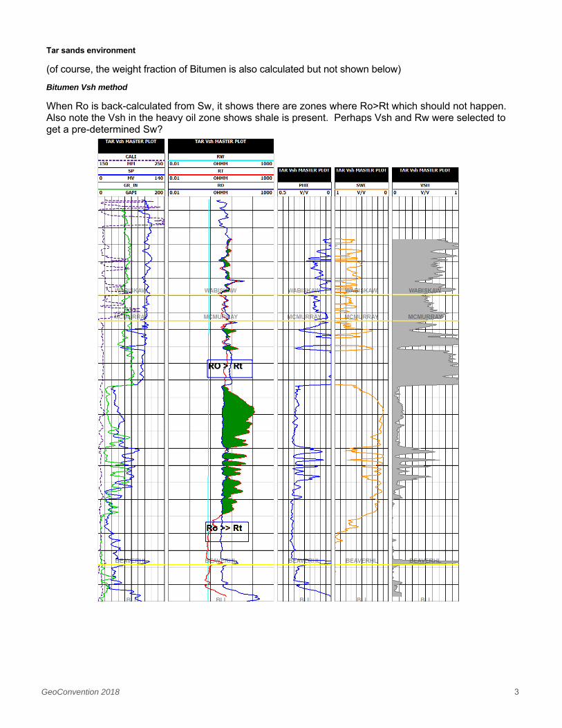
Tar sands environment
(of course, the weight fraction of Bitumen is also calculated but not shown below)
Bitumen Vsh method
When Ro is back-calculated from Sw, it shows there are zones where Ro>Rt which should not happen. Also note the Vsh in the heavy oil zone shows shale is present. Perhaps Vsh and Rw were selected to get a pre-determined Sw?

GeoConvention 2018 4
Bitumen, heavy oil, EM method
Here, Ro ~ Rt in shales. Also, the heavy oil zone has no clay. The Free porosity shows oil is moveable, even though measurements show very high viscosity.

GeoConvention 2018 5
Lithic Mannville environment
Vsh method
Note that Rw (0.2@FT) and Vsh (~30%) are ‘manipulated’ to obtain an “acceptable” Sw of about 30%. No perm is presented as there was no core to calibrate to. Ro ~ Rt, but there is no continuity in the Ro curve, due to abrupt changes in Rw.

GeoConvention 2018 6
EM method
Pass 1
The addition of predicted NMR curves enhances the output, providing permeability (KSDR), bound fluid volume for irreducible saturation (S_BFV) and an estimate of producibility from the F_logs (formation_factors * Rw) (i.e. Ro_TCMR, Ro_CMRP).
The right-most mineral plot shows a more complex mineralogy, with traces of pyrite and small fractions of dolomite and calcite, as well as muscovite (mica). Incidentally, discontinuous pyrite does not affect resistivity.
Rw is ~ 0.1@25C, according to Susan Johnson, Opus Engineering, [salinity expert]. Our Rw matches hers. Note the Ro matches on the lowest values to Rt, due to vertical resolution differences between density and IDPH.
Free porosity is shown in the resistivity track, comparing Ro_CMRP to Rt. Well should flow.
Invasion shows that SFLU>IDPH, agrees with free porosity.

GeoConvention 2018 7

GeoConvention 2018 8
Pass 2
However, a higher Rw, 0.1@FT, was used to obtain similar Sw (~30%) as the Vsh model. This was accomplished by multiplying the SP by 0.5.
Also note the clay in the pay zone is almost zero (~ 5%). There is some dolomite (~5%).
Note the free porosity is no longer seen. This is an indication that the Rw is too high (use 0.246@25C, rather than 0.1@25C).
This example is a clear case for a Dielectric tool to provide the correct Rw, without question. (Ref. 14)

GeoConvention 2018 9

GeoConvention 2018 10
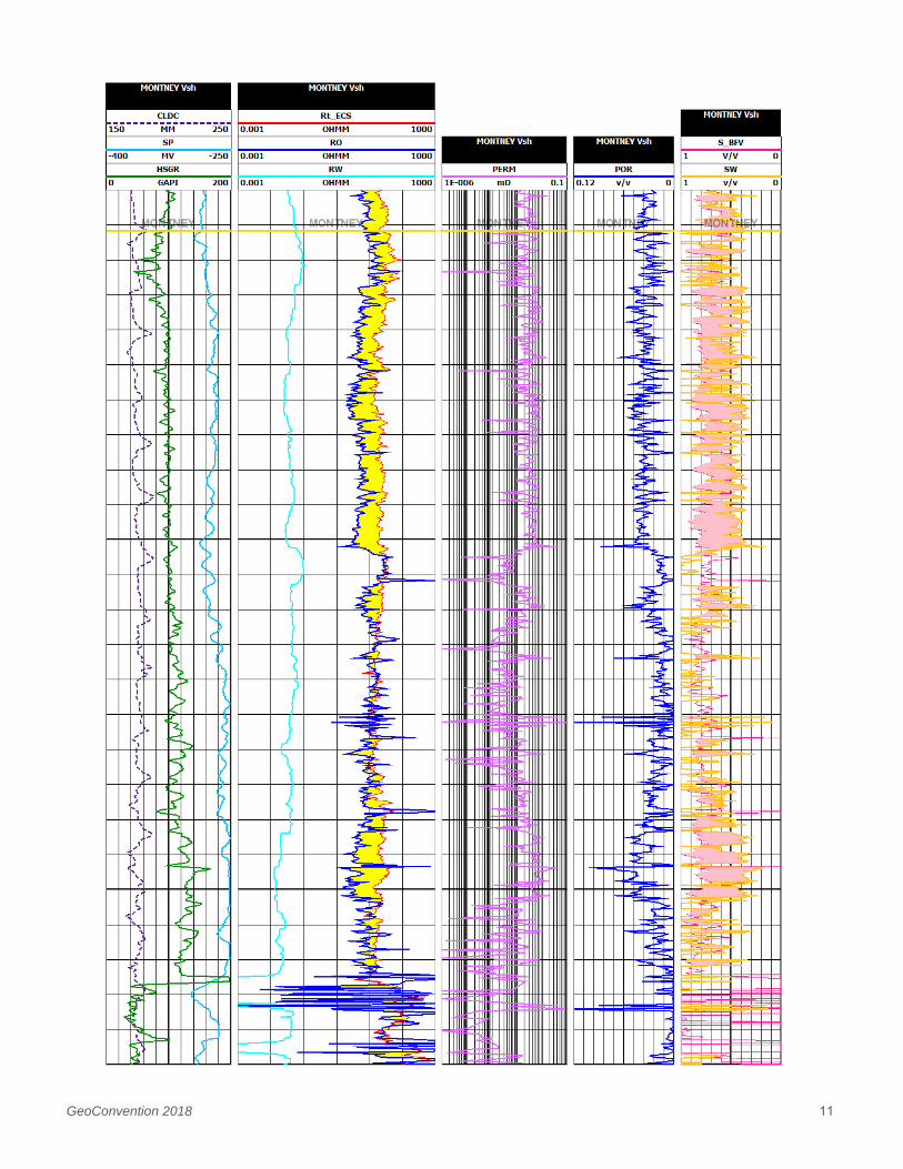
Unconventional shale, Montney environment
Offset-core method
This is not really a Vsh method nor an EM method. It is an offset-core method from another well. The curves were computed relying heavily on core using Dean Stark methods. Core was carefully preserved. Note also the Sw is higher than the Sw from the EM method: the back-calculated Rw is higher for the offset-core method. There are a couple of caveats:
1) The Sw was computed from a formula (Ref. 12) that does not involve Rw. The Dean Stark core work was not on this well. Question, does the offset-core analysis on another well, apply to this well? RCA core Sw is much lower (Appendix 3), so that answers the question: the transform does not necessarily apply for Sw, or permeability on a different well. However, it does apply for porosity. Hence, using core does not result in a transportable interpretation. That is why we use the EM methods. EM methods are transportable.
2) The Ro and Rw shown are a reverse-calculation of Sw, using an Archie formula with m=n=M_ZERO and a Ghanbarian formation factor (Ref. 9).
3) The mineralogy has to be imagined from offset-core on another well. Vsh was not used in the computation. Offset-core analysis was.
GeoConvention 2018 11
GeoConvention 2018 12
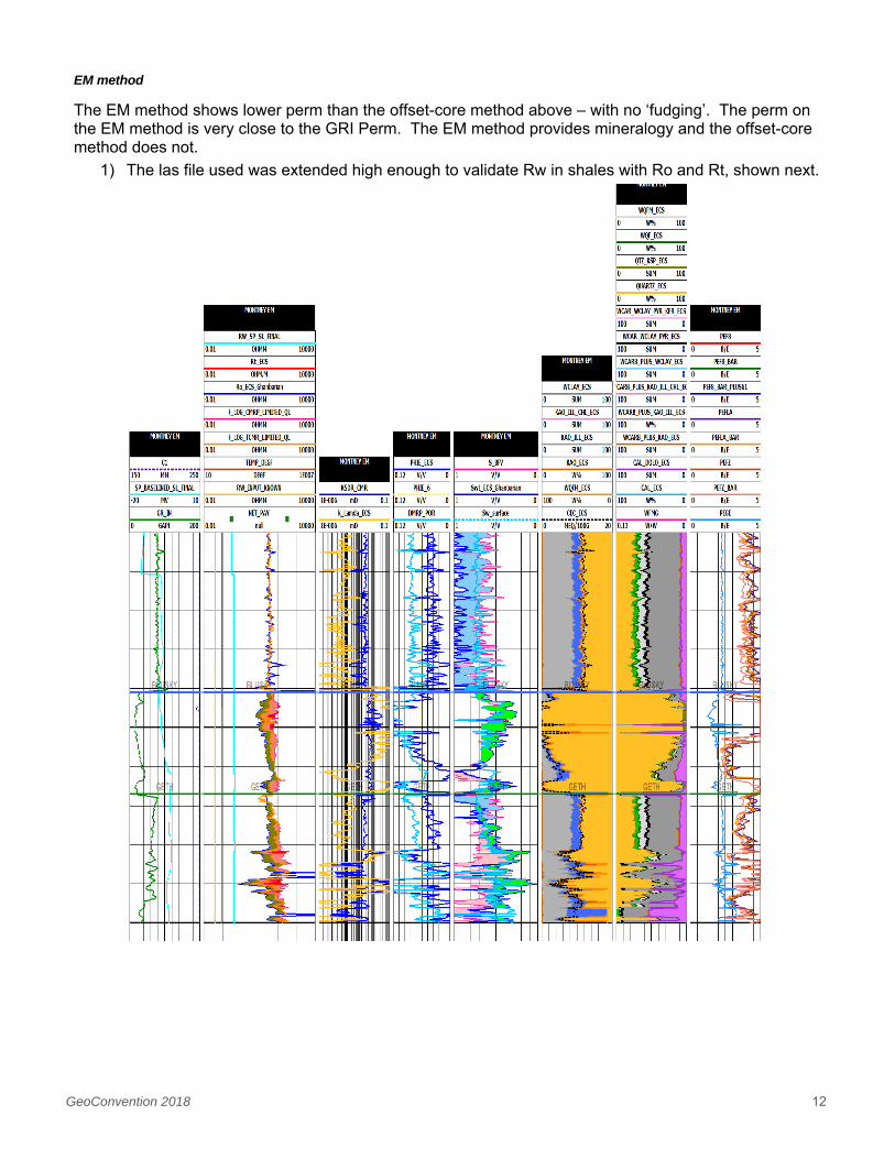
EM method
The EM method shows lower perm than the offset-core method above – with no ‘fudging’. The perm on the EM method is very close to the GRI Perm. The EM method provides mineralogy and the offset-core method does not.
1) The las file used was extended high enough to validate Rw in shales with Ro and Rt, shown next.
GeoConvention 2018 13
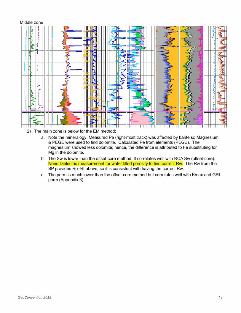
Middle zone
2) The main zone is below for the EM method;
a. Note the mineralogy: Measured Pe (right-most track) was affected by barite so Magnesium & PEGE were used to find dolomite. Calculated Pe from elements (PEGE). The magnesium showed less dolomite; hence, the difference is attributed to Fe substituting for Mg in the dolomite.
b. The Sw is lower than the offset-core method. It correlates well with RCA Sw (offset-core). Need Dielectric measurement for water filled porosity to find correct Rw. The Rw from the SP provides Ro=Rt above, so it is consistent with having the correct Rw.
c. The perm is much lower than the offset-core method but correlates well with Kmax and GRI perm (Appendix 3).

GeoConvention 2018 14

GeoConvention 2018 15
Milk River Alderson -- distal to foreshore environment
Vsh method.
Note the shifted neutron of -15 pu is used to find the gas zones. Porosity and Permeability using the Nieto formula works nicely. Vsh was derived by an “expert” Vsh Consultant: Vsh is the minimum of GR, N-D and conductivity. Rw and Ro were back-calculated. The Buckles formula was used for Sw to avoid having to know Rw. However, note that Ro and RESD do not match above Milk River, as they should, if the clay compensation was correct.
GeoConvention 2018 16
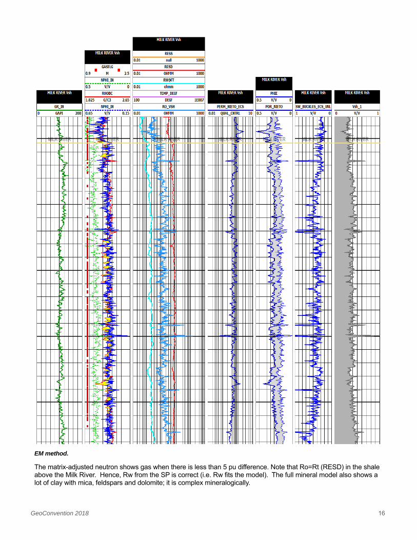
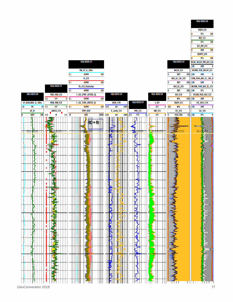
EM method.
The matrix-adjusted neutron shows gas when there is less than 5 pu difference. Note that Ro=Rt (RESD) in the shale above the Milk River. Hence, Rw from the SP is correct (i.e. Rw fits the model). The full mineral model also shows a lot of clay with mica, feldspars and dolomite; it is complex mineralogically.
GeoConvention 2018 17
GeoConvention 2018 18
In summary, the key to finding pay zones in the Milk River (and Alderson) is to shift the field neutron by -15 porosity units and look for cross-over with the density porosity. In the EM model, gas occurs when the matrix adjusted curves separate by less than 5 pu. Note the CEC falls close to the WCLAY, because the clay is computed as mainly illite with a CEC of 25 meq/l; hence, on the scale selected of 0-20 meq/l, the CEC happens to fall near the Wclay.
Appendix 1 has a Cretaceous sand environment to illustrate how to obtain the formation water resistivity from the spontaneous potential. This method differs from past practice, where deflection was measured from a shale baseline. Now, the SP deflection is measured from a calculated zero. Furthermore, the SP is corrected for drift usually caused by the casing that short-circuits the return to the mud fish. All the EM examples utilize this method to determine Rw. The reason is, when the resistivity has been corrected by CEC, the Ro can be compared to Rt and in a shale [with no organic carbon]; the Ro must equal Rt, thus ensuring that the correct Rw has been implemented. The Vsh method makes this verification very difficult, since the Vsh does not exactly correct the Ro in shales.
Conclusions
The EM method is an updated method from the Vsh method. As such, there are additional routines available that result in a more complete computation, resulting in improved water saturation, porosity, permeability and net to gross results.
The Vsh and EM methodologies are just different methods to do the same thing: correct for clay effects on water saturation, porosity and permeability. Science has yielded formulas like Shell’s Waxman-Smits-Thomas and Schlumberger’s Dual Water; empiricism has provided Simandoux, Indonesian and modified Dual Water plus localized adaptations. Universal models only [seem to] exist when one applies EM. Any model can be improved with localized adaptations to core measurements.
When should one use Vsh instead of element to mineral methods?
1) If 6000 wells, use Vsh and check key wells with EM. One probably only wants to find sweet spots. The preparation involved in estimating missing data when only triple combo logs have been run, is too time consuming for more than 10-30 wells at a time.
2) If no prediction of missing curves is possible, use Vsh. I use Geological Analysis by Maximum Likehood Systems (GAMLS, Ref. 1) to predict missing data as it is easy and accurate.
3) If no knowledge of ECS/Flex/Gem nor of NMR, use Vsh. There is a learning curve to EM methods. Contact author.
4) If Vsh is “good enough”, use Vsh.
5) If Vsh software is all you have, use Vsh.
6) If there is core with excellent measurements, derive equations directly from the core (as John Nieto, Canbriam Energy Inc., does, Ref. 12; “We were very careful with our core acquisition for D-S. OBM, Sleeved core, end capped, Shipped chilled to Lab (not frozen), Immediate plug cutting (2am!), Immediate immersion in Soxhlet extractors, Dummy plugs, Clean toluene. Months of cleaning , then drying. (per AAPG))”
7) One can think of the EM method as just a way to get the equivalent of Vsh in units that are more related to the rock and can be cross-checked with core. In summary, we use what is available and do the best we can. For me, that is EM. For others it is core or Vsh.

GeoConvention 2018 19
The addition of a Dielectric measurement to assist with Rw would be useful in all cases, when seeking the truth.
Acknowledgements
Aminex PLC has graciously provided permission to publish using some of their data. “I am more than happy for you to publish your findings and I am always happy to further the technical abilities of our industry. A nice mention or acknowledgement of Aminex .... doesn't hurt either!”
The rest of the data was obtained via sources that provide released information.
References
1) Eslinger, E., and R. V. Everett, 2012, ‘Petrophysics in gas shales’, in J. A. Breyer, ed., Shale Reservoirs—Giant resources for the 21st century: AAPG Memoir 97, p. 419–451.
2) Eslinger, E., and Boyle, F., ‘Building a Multi-Well Model for Partitioning Spectroscopy Log Elements into Minerals Using Core Mineralogy for Calibration’, SPWLA 54th Annual Logging Symposium, June 22-26, 2013.
3) M. M. Herron, SPE, D. L. Johnson and L. M. Schwartz, Schlumberger-Doll Research, ‘A Robust Permeability Estimator for Siliciclastics’, SPE 49301, 1998 SPE Annual Technical Conference and Exhibition held in New Orleans, Louisiana, 27–30 September 1968.
4) Susan L. Herron and Michael M. Herron, ‘APPLICATION OF NUCLEAR SPECTROSCOPY LOGS TO THE DERIVATION OF FORMATION MATRIX DENSITY’ Paper JJ Presented at the 41st Annual Logging Symposium of the Society of Professional Well Log Analysts, June 4-7, 2000, Dallas, Texas.
5) Clavier, C., Coates, G., Dumanoir, J., ‘Theoretical and Experimental Basis for the Dual-Water Model for interpretation of Shaly Sands’, SPE Journal Vol 24 #2, April 1984.
6) Herron, M.M, ‘Geochemical Classification of Terrigenous Sands and Shales from Core or Log Data’, Journal of Sedimentary Petrology, Vol. 58, No. 5 September 1988, p. 820-829.
7) Everett, R.V., Berhane, M, Euzen, T., Everett, J.R., Powers, M, ‘Petrophysics Designed to Honour Core – Duvernay & Triassic’ Geoconvention Focus May 2014.
8) Everett, R. V. ‘London Petrophysical Society June Newsletter 2017’.
9) Ghanbarian, B, Hunt, A. g., Ewing, R. P. Skinner, T. E., ‘Universal scaling of the formation factor in porous media derived by combining percolation and effective medium theories’ Geophysical Research letters, 10./2014GL060180, [email protected]
10) Herron, S. L., Herron, M. M., Pirie, Iain, Saldungaray, Craddock, Paul, Charsky, Alyssa, Polyakov, Marina, Shray, Frank, Li, Ting, ‘Application and Quality Control of Core Data for the Development and Validation of Elemental Spectroscopy Log Interpretation’, SPWLA, 55th Annual Logging Symposium, Abu Dhabi, United Arab Emirates, May 18-22, 2014.
11) Freedman, R., Min, C. C., Gubelin, G., Freeman, J. J., McGuiness, T., Terry, R., Rawlence, D., ’Combining NMR and Density Logs for Petrophysical Analysis in Gas-Bearing Formations’. SPWLA 1998.
12) Nieto, J., Bercha, R., Chan, J., ‘Shale Gas petrophysics – Montney and Muskwa, are they Barnett look-alikes?’ SPWLA JUNE 21-24, 2009
13) Everett, R. V. ‘Steps to compute using PDHC’ CWLS Advanced Interpretation School May, 2017-2018 notes.
GeoConvention 2018 20
14) Decoster, E., Faivre, O., Carmona, R., ‘Application of a New Array Dielectric Tool to the Characterization of Orinoco Belt Heavy Oil Reservoirs’. IAPG, 2008.
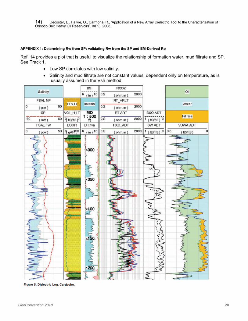
APPENDIX 1: Determining Rw from SP: validating Rw from the SP and EM-Derived Ro
Ref. 14 provides a plot that is useful to visualize the relationship of formation water, mud filtrate and SP. See Track 1.
Low SP correlates with low salinity.
Salinity and mud filtrate are not constant values, dependent only on temperature, as is usually assumed in the Vsh method.

GeoConvention 2018 21
What can we do without a Dielectric log to obtain an Rw? Follow this procedure. We assume the RMF is constant changing only with temperature. Then we find a variable Rw based on SP deflections.
Step 1
A value for the “known Rw” is calculated. A known Rw can come from an estimate, water catalog, DST, formation tester, etc. It represents an Rw at only one depth in the well that samples were taken from. Our estimate for this well is to solve for Rw assuming 100% Sw in a zone below the gas/water contact. Remember this value will be cross-checked later so we do not have to be precisely accurate at this stage. For Rw_known, use 0.2 at formation temperature (~ 110C (230F)). In the formulas, “TEMP_DEGF” is some version of 0.0198*DEPTHFT+42.805, that provides a bottom hole reservoir temperature that is estimated about 10 to 20 degrees F above the highest log-recorded temperature [the hole temperature is less because of mud circulation, of course].
Then Rw_known=0.2*(230+6.77)/(TEMP_DEGF+6.77).
Also calculate Rmf from a temperature gradient, [RMF]*([measured temperature] +6.77)/(TEMP_DEGF+6.77).
Also, Rw of 0.05@308F, 0.05*(308+6.77)/(TEMP_DEGF+6.77); this value is a “ballpark” for all reservoirs and happens to be the value for the Cardium, by serendipity. We will use it only to get an approximate zero line, rather than using a shale baseline.
Step 2
The next step is to find SP_ZERO. You solve for it from SP_ZERO_CALC=-k*log(RMF/RW_05). This will not give an exact zero average over the interval but will get you into the ballpark. Note we do not use a shale baseline for a zero line; we want a non-zero Rw in shales as well as sands. The first attempt is:

GeoConvention 2018 22
Note the above calculated value does not average at zero as the left and right values are 42 and 56. Now, add a constant until the left and right average values are the same. i.e. the average is zero over the interval selected, such as -3 and +3 averages.
The plot above shows the left and right values on the plot are the same, so the average is zero. This is where you want to be. Now plot Rw_05, RW_KNOWN and Rt on the log track; plus, SP [SPDL], SP_ZERO_CALC and temperature in the left, linear track.
Now plot an initial Rw_SP_CALC and see how close it comes to the Rw_KNOWN_POINT2. Keep changing SP_SHIFT_CALC until Rw_SP_CALC just touches Rw_KNOWN_POINT2. The formulas are:
We apply another "ADD" to SP_SHIFT_CALC to move the RW_SP_CALC to the right. This is trial and error until we get the two curves to agree at the arrow. Using 0.2, we must apply a shift to the right. By trial and error, we find that a shift of +245mv seems to work OK. Arrow shows where we match.
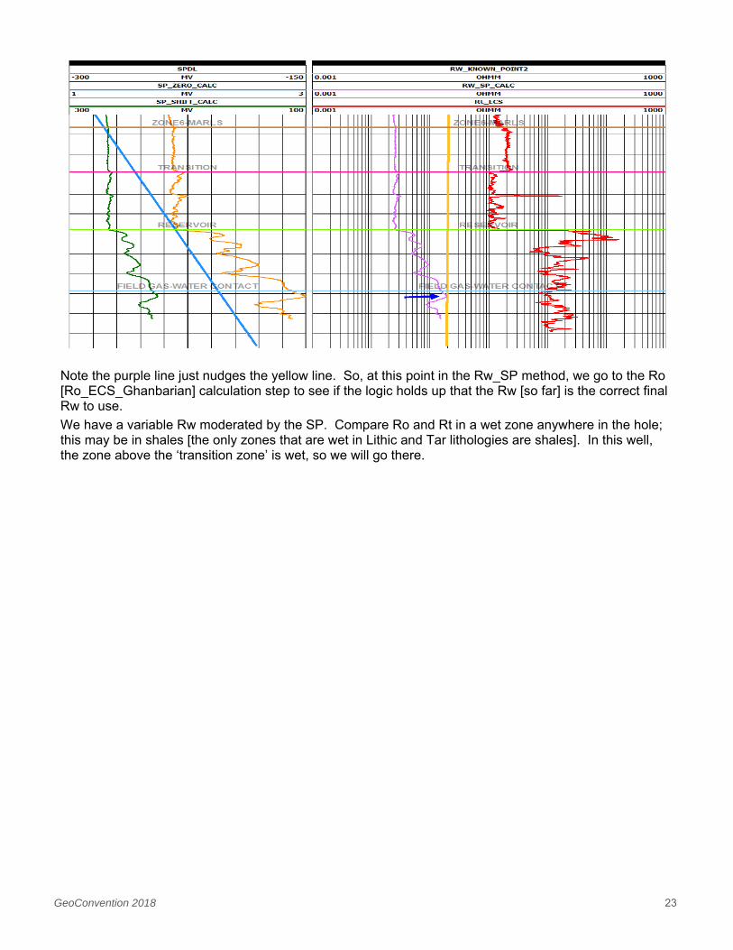
GeoConvention 2018 23
Note the purple line just nudges the yellow line. So, at this point in the Rw_SP method, we go to the Ro [Ro_ECS_Ghanbarian] calculation step to see if the logic holds up that the Rw [so far] is the correct final Rw to use.
We have a variable Rw moderated by the SP. Compare Ro and Rt in a wet zone anywhere in the hole; this may be in shales [the only zones that are wet in Lithic and Tar lithologies are shales]. In this well, the zone above the ‘transition zone’ is wet, so we will go there.

GeoConvention 2018 24
Our result shows that Ro is too low compared to Rt in the wet Marl zone; therefore, the Rw must be too low. Note that the water saturation is not 100% (i.e. Ro<Rt) at the field gas water contact, even though water is produced. The reason the field produces water from this zone is that [NMR, CMRTM] “free porosity” is greater than the hydrocarbon filled porosity (CMRP>HCPV). Hence, there is free water. In addition, the free water is fresher than water in the gas zone. The fresh water probably comes from meteoric water since the higher the Sw, the higher the relative perm is to water. Having meteoric water appears to be common in a rift basin. Also, meteoric water is common in the Belly River, Mannville and Milk River of the Western Canadian Sedimentary Basin.
Now cycle, try SP_SHIFT_CALC have a value added to them. Not “rocket science”, just paste an "add" and try:
1) SP_SHIFT_CALC, ADD 10 (Rw too low)
keep cycling...2, 3, 4, etc., until you get Rw acceptable:
1) SP_SHIFT_CALC, ADD an amount to make Rw acceptable. Our check that we have the correct Rw, is to ensure that in the resistivity of the entire interval, Ro <= Rt. Note the transition zone has Ro<Rt as we would expect since there are hydrocarbons in the transition zone. Immediately above the transition zone, we have Ro very close to Rt indicating the zone is wet. The point of the exercise is that one should review the entire well that one has available. One must allow for SP drift, especially as one approaches casing. One can see that the correct Rw is not 0.2 but rather 0.08 at formation temperature at the blue arrow. In the pay zone, Rw is about 0.02 at temperature.
2) If one is convinced the RW_KNOWN is correct, then one may have to squeeze the amplitude of the SP deflection to obtain a fit. In cases of the Lithic environment, muds are very fresh, and the SP deflection is huge, but the SP equation is beyond its limit of a dilute NaCl environment, custom analysis may be needed. The same methodology applies. Just reduce the deflection amplitude to fit the data.
Result looks like:

GeoConvention 2018 25
In summary, this is a powerful method. We are privileged to have it coded.
APPENDIX 2 Ghanbarian code
For utility of readers familiar with code who may like to update, the Ghanbarian formation factor is presented in coding language, since the formulas may not be as clear in the paper. One can just cut and paste or modify to suit one’s code (Ref. 9). In summary, the Ghanbarian formation factor provides an improved formation factor relationship, based on Percolation theory, so we have chosen to use it. The variable “ba5” is total porosity determined from the EM-derived grain density.
The variable “$c$501” is an option to use the formation factor or not.

GeoConvention 2018 26
Readers who want more detail are advised to contact James Everett, MSc., jamie@everett-energy_software.com