Vortex_Khwaja Saleem a
30
1 Vortex Shedding from a Cylinder & Data Acquisition Research Methods (MACE 61078) Khwaja Saleem Fathimulla (8281580) Group ‘B’ 11 th November 2011 MSc Aerospace Engineering School of Mechanical, Aerospace and Civil Engineering The University of Manchester
-
Upload
khwaja-saleem -
Category
Documents
-
view
224 -
download
0
Transcript of Vortex_Khwaja Saleem a
8/3/2019 Vortex_Khwaja Saleem a
http://slidepdf.com/reader/full/vortexkhwaja-saleem-a 1/30
1
Vortex Shedding from a Cylinder & Data Acquisition
Research Methods (MACE 61078)
Khwaja Saleem Fathimulla (8281580)
Group ‘B’
11th
November 2011
MSc Aerospace Engineering
School of Mechanical, Aerospace and Civil Engineering
The University of Manchester

8/3/2019 Vortex_Khwaja Saleem a
http://slidepdf.com/reader/full/vortexkhwaja-saleem-a 2/30
2
LIST OF CONTENTS
Objectives………………………………………………………… 5
Introduction……………………………………………………….. 5
Experimental Apparatus…………………………………………... 7
Experimental Procedure…………………………………………... 11
Presentation of results…………………………………………….. 12
Calculations……………………………………………………….. 22
Discussion of Results……………………………………………... 27
Conclusion……………………………………………………….... 28
Acknowledgements………………………………………………... 28
References………………………………………………………… 28
Appendix A………………………………………………………... 29

8/3/2019 Vortex_Khwaja Saleem a
http://slidepdf.com/reader/full/vortexkhwaja-saleem-a 3/30
3
LIST OF FIGURES:
Figure 1: Von Karman vortex street behind a cylinder…………………… 6
Figure 2: The wind tunnel………………………………………………….7
Figure 3: Circular cylinder…………………………………………………7
Figure 4: Hotwire Anemometer……………………………………………8
Figure 5: The Micromanometer……………………………………………8
Figure 6: Personal Computer………………………………………………8
Figure 7: The rotary regavolt………………………………………………9
Figure 8: The traverse gears……………………………………………….. 9
Figure 9: The spectrum analyser…………………………………………...10
LIST OF TABLES:
Table 1: Sample data set (at 700 Hz with 1024 samples)…………………12
Table 2: Vortex shedding measurements………………………………….22
Table 3: Calibration table………………………………………………… 23

8/3/2019 Vortex_Khwaja Saleem a
http://slidepdf.com/reader/full/vortexkhwaja-saleem-a 4/30
4
NOMENCLATURE
d Diameter of the cylinder, m
f Vortex shedding frequency,Hz
f s Sampling frequency,Hz
n Number of samples
PDF probability distribution function
RMS root mean square,m/s
RTI relative turbulence intensity
St Strouhal number
T time,sec
Density, kg/m3
Dynamic viscosity, kg/(m.s)
U Total instantaneous velocity,m/s
U1 Mean velocity,m/s
u’ Fluctuating velocity,m/s
8/3/2019 Vortex_Khwaja Saleem a
http://slidepdf.com/reader/full/vortexkhwaja-saleem-a 5/30
5
Objectives:
• To obtain an optimum sample frequency from Von Karman vortex data produced by a
circular cylinder.
• To compare optimum sample frequency with under and over sampling frequencies.
Introduction:
The flow field over the cylinder is symmetric at low values of Reynolds number. As the
Reynolds number increases, flow begins to separate behind the cylinder causing vortex shedding
which is an unsteady phenomenon. The Reynolds number is given as the ratio of inertial force to
viscous forces:
=
Where,
is density in, kg/m3;
free stream velocity, in m/s;
d diameter of the cylinder, in m;
viscosity, in kg/(m.s).
When we consider a circular cylinder under a turbulent flow the pressure increases past the
cylinder and the unsteady boundary layer breaks away on the downstream side to form a pair of travelling vortices. These vortices have different frequencies and shed alternately from the
surface. This is called a Von Karman Vortex Street. The relation between the vortex shedding
frequency and Reynolds number(Re) is :
= 0.198(1− . )
Where the Strouhal number is: St =
(f is the vortex shedding frequency).

8/3/2019 Vortex_Khwaja Saleem a
http://slidepdf.com/reader/full/vortexkhwaja-saleem-a 6/30
6
t
t/2
There are two types of frequencies produced near to the centre line because of alternate vortices
are given as: f and 2f (corresponding to 1/t and 1/(t/2), respectively).
For the data analysis: velocity from Hotwire Anemometer is given as:
U = U1 + u’
Where U1 is the total instantaneous velocity, U1 is the mean velocity and u ’ is the fluctuation
component of velocity.
Mean velocity id given as:
U1 =
To calculate the RMS(root mean square) we need to subtract the mean velocity component U1
from each instantaneous velocity value, Ui, square the result and add such results. Now take the
square root of the sum of all such terms divided by n.
RMS (u’) = ( − 1) 2 = − ( ) 2
Lastly, the relative turbulence intensity (RTI) is given as:
RTI =()
×100%

8/3/2019 Vortex_Khwaja Saleem a
http://slidepdf.com/reader/full/vortexkhwaja-saleem-a 7/30
7
Experimental Apparatus:
1) Wind Tunnel
The wind tunnel we used was a bench wind tunnel; the test section was around 300mm long and
300 width in dimensions.
2) Circular Cylinder (test specimen)
Figure shows a horizontal circular cylinder which is our test section.
3) Hotwire Anemometer
This is placed behind the cylinder. Hotwire Anemometer is made of tungsten with a
length of 2mm and diameter of 5 . As shown in the figure below.

8/3/2019 Vortex_Khwaja Saleem a
http://slidepdf.com/reader/full/vortexkhwaja-saleem-a 8/30
8
4) Micromanometer
5) Computer
The velocity histogram was produced by the help of software which was installed in the
computer. Software helped to calibrate and receive signal.

8/3/2019 Vortex_Khwaja Saleem a
http://slidepdf.com/reader/full/vortexkhwaja-saleem-a 9/30
9
6) The Rotary Regavolt
This is used to vary the voltage, it is located below the wind tunnel.
7) The traverse gears
This is used to change the position of the Hotwire Anemometer across the vertical axis of the
cylinder.
8/3/2019 Vortex_Khwaja Saleem a
http://slidepdf.com/reader/full/vortexkhwaja-saleem-a 10/30
10
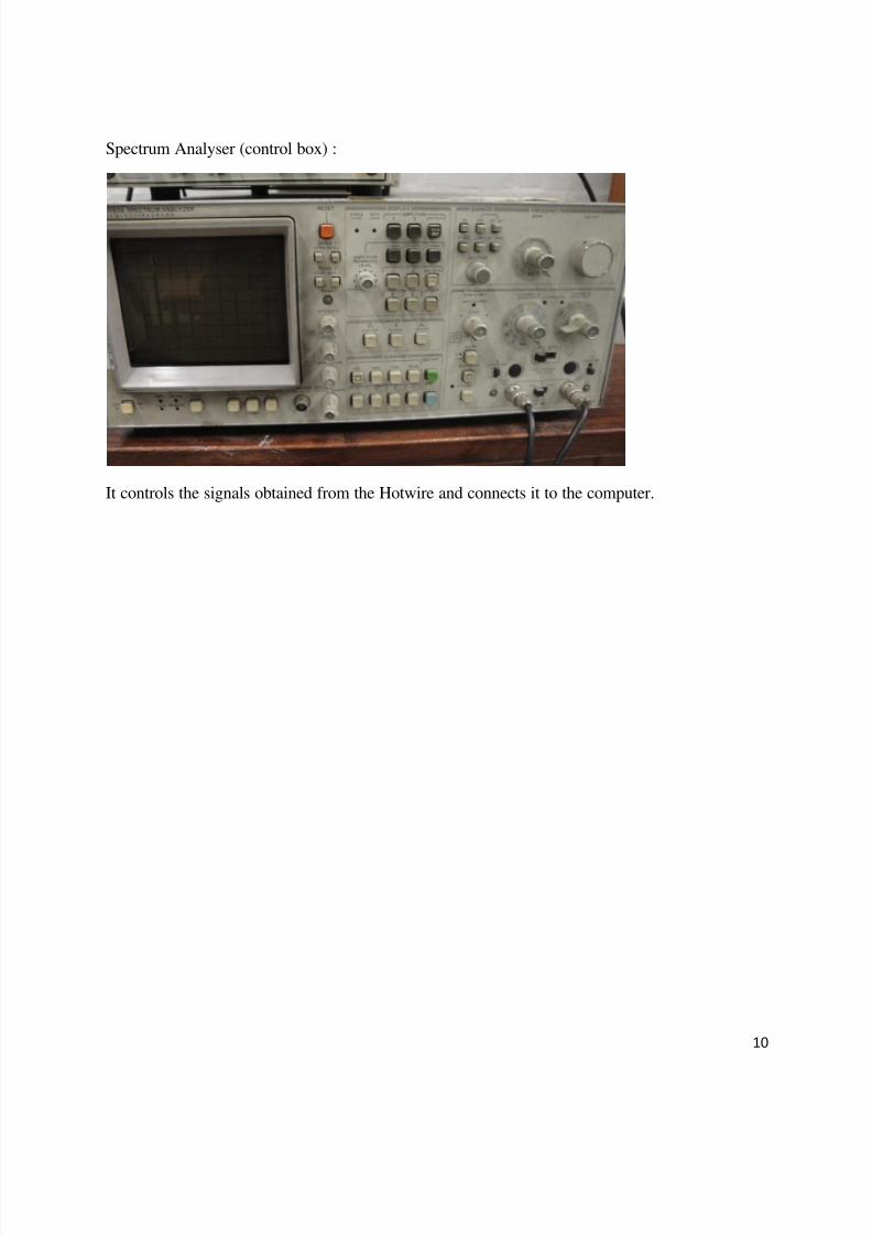
Spectrum Analyser (control box) :
It controls the signals obtained from the Hotwire and connects it to the computer.

8/3/2019 Vortex_Khwaja Saleem a
http://slidepdf.com/reader/full/vortexkhwaja-saleem-a 11/30
11
Experimental Procedure:
First we calibrate the hot-wire anemometer over a suitable velocity range(10m/s) , note down the
initial voltage of the hot-wire probe which corresponds to ‘0’ velocity. Then regularly increase
the velocity of air inside the wind tunnel we obtain different pressure values which are later
initialized in lab-view software. The lab-view software in return provides the velocity and
voltage of that pressure at every interval. We know that: the relation between voltage output
generated (E) and the velocity (U) is given below:
(E-Eo)2
= BUn
Where E(volts) is the voltage corresponding to the velocity U(m/s), Eo is the voltage at zero
velocity and B,n are constants.
The software produce a graph that shows the variation of velocities across the square of the
voltage differences (E-Eo)2.
After calibration, the optimum , under and over sampling frequencies must be calculated. For
this the hot wire is placed at the centre of the cylinder. The frequency is obtained by using the
Strouhal number equation. After which the maximum frequency and sampling frequency is
calculated similarly. The sampling rate should be 2.5 times the maximum frequency present in
the signal and the number of samples per second should be of order 2n. Optimum sampling rate is
is 700(appox.) and set number of samples collected per second to 1024 at the closest power of 2
for 700. (Calculations in next section). Similarly we record date for over and under sampling.
Keeping the sampling rate at 1400 Hz with 211
samples per second and 350 Hz with 29
samples
per second for over and under sampling frequency respectively.
We use the traverse gear to change the position of the hotwire probe. For each 10 mm
displacement the software measures and record the instantaneous velocity. At 100 mm the
readings were declined.
Finally note all data required using Microsoft Excel to analysis over and under sampling; to view
the variation of the frequency spectra, mean and RMS velocities and RTI across wake.

8/3/2019 Vortex_Khwaja Saleem a
http://slidepdf.com/reader/full/vortexkhwaja-saleem-a 12/30
12
Presentation of Results:
Table 1: Sample data (at centre of the cylinder, taken at 700hz with 1024 samples per second
Voltage
E(volts)
E-Eo
(volts)
(E-Eo)2
(volts)2
Velocity
(m/s)
3.637695 1.021945 1.044373 9.675407
3.635254 1.019504 1.039389 9.622973
3.564453 0.948703 0.900038 8.183571
3.554687 0.938938 0.881604 7.997011
3.620605 1.004856 1.009735 9.312362
3.566895 0.951145 0.904676 8.230654
3.535156 0.919406 0.845308 7.632313
3.505859 0.89011 0.792295 7.105908
3.422852 0.807102 0.651413 5.743165
3.708496 1.092746 1.194094 11.281222
3.654785 1.039035 1.079594 10.047832
3.505859 0.89011 0.792295 7.105908
3.530273 0.914524 0.836353 7.542872
3.686523 1.070774 1.146556 10.764926
3.701172 1.085422 1.178141 11.107291
3.664551 1.048801 1.099983 10.264921
3.688965 1.073215 1.15179 10.821481
8/3/2019 Vortex_Khwaja Saleem a
http://slidepdf.com/reader/full/vortexkhwaja-saleem-a 13/30
13
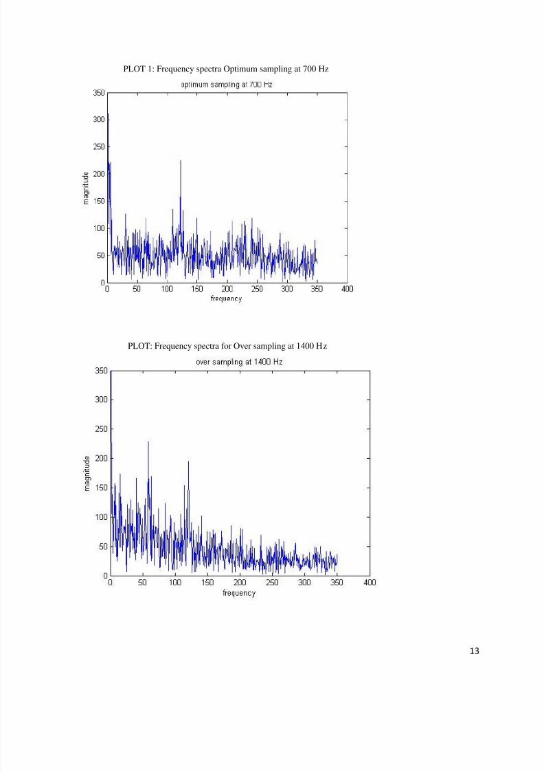
PLOT 1: Frequency spectra Optimum sampling at 700 Hz
PLOT: Frequency spectra for Over sampling at 1400 Hz

8/3/2019 Vortex_Khwaja Saleem a
http://slidepdf.com/reader/full/vortexkhwaja-saleem-a 14/30
14
PLOT 3: Frequency Spectra for under sampling at 350 Hz
The following graphs represent Frequency spectra across the wake:

8/3/2019 Vortex_Khwaja Saleem a
http://slidepdf.com/reader/full/vortexkhwaja-saleem-a 15/30
15

8/3/2019 Vortex_Khwaja Saleem a
http://slidepdf.com/reader/full/vortexkhwaja-saleem-a 16/30
16
8/3/2019 Vortex_Khwaja Saleem a
http://slidepdf.com/reader/full/vortexkhwaja-saleem-a 17/30
17
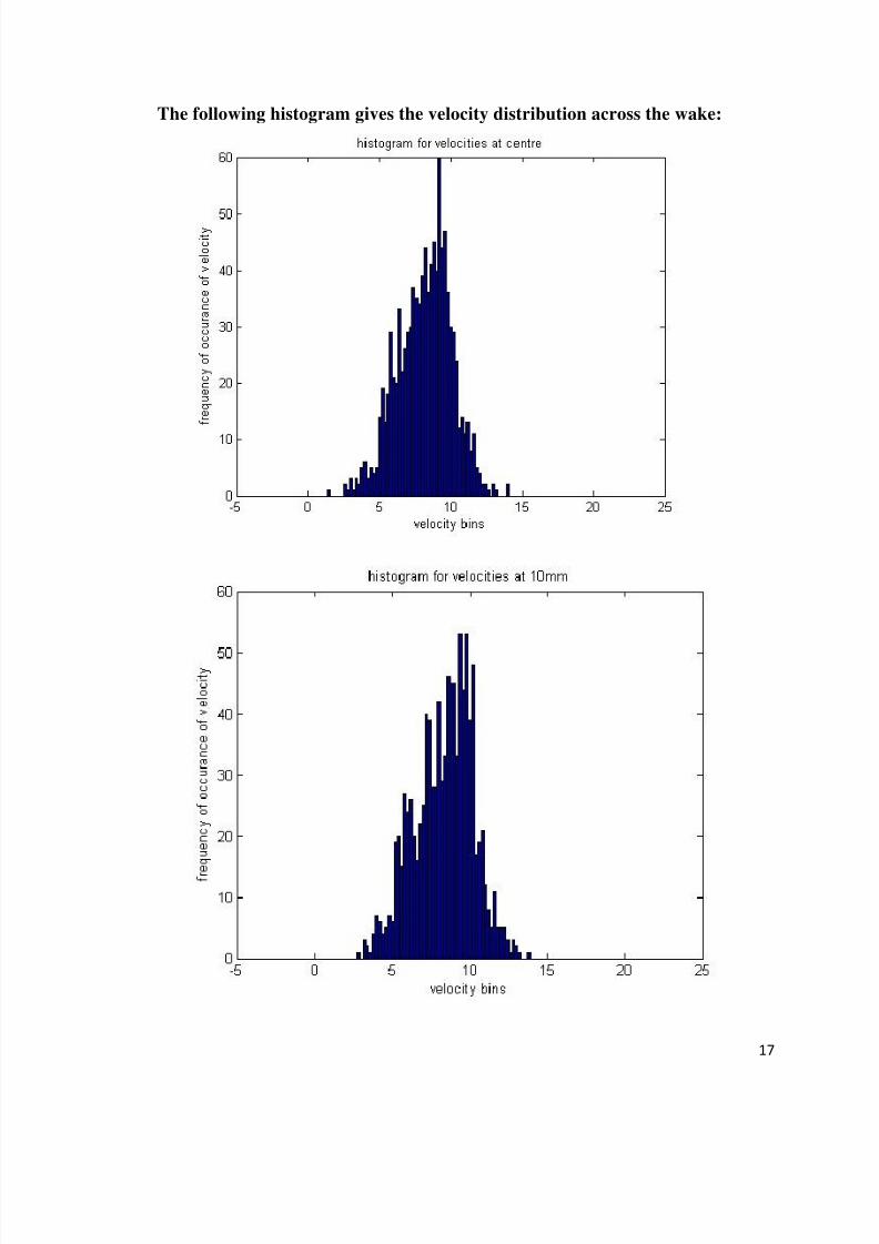
The following histogram gives the velocity distribution across the wake:

8/3/2019 Vortex_Khwaja Saleem a
http://slidepdf.com/reader/full/vortexkhwaja-saleem-a 18/30
18

8/3/2019 Vortex_Khwaja Saleem a
http://slidepdf.com/reader/full/vortexkhwaja-saleem-a 19/30
19

8/3/2019 Vortex_Khwaja Saleem a
http://slidepdf.com/reader/full/vortexkhwaja-saleem-a 20/30
20

8/3/2019 Vortex_Khwaja Saleem a
http://slidepdf.com/reader/full/vortexkhwaja-saleem-a 21/30
21
PLOT 6: Umean and Urms profile across the wake:
8/3/2019 Vortex_Khwaja Saleem a
http://slidepdf.com/reader/full/vortexkhwaja-saleem-a 22/30
22
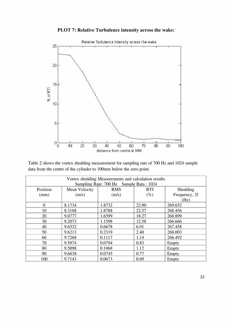
PLOT 7: Relative Turbulence intensity across the wake:
Table 2 shows the vortex shedding measurement for sampling rate of 700 Hz and 1024 sample
data from the centre of the cylinder to 100mm below the zero point.
Vortex shedding Measurements and calculation resultsSampling Rate: 700 Hz Sample Bata : 1024
Position
(mm)
Mean Velocity
(m/s)
RMS
(m/s)
RTI
(%)
Shedding
Frequency, 2f
(Hz)
0 8.1734 1.8732 22.90 269.652
10 8.3168 1.8788 22.57 268.456
20 9.0777 1.6599 18.27 268.899
30 9.2073 1.1598 12.58 266.666
40 9.6532 0.6678 6.91 267.458
50 9.6213 0.2319 2.40 268.003
60 9.7268 0.1117 1.14 266.492
70 9.5974 0.0794 0.83 Empty
80 9.5098 0.1068 1.12 Empty
90 9.6638 0.0745 0.77 Empty
100 9.7143 0.0673 0.69 Empty
8/3/2019 Vortex_Khwaja Saleem a
http://slidepdf.com/reader/full/vortexkhwaja-saleem-a 23/30
23
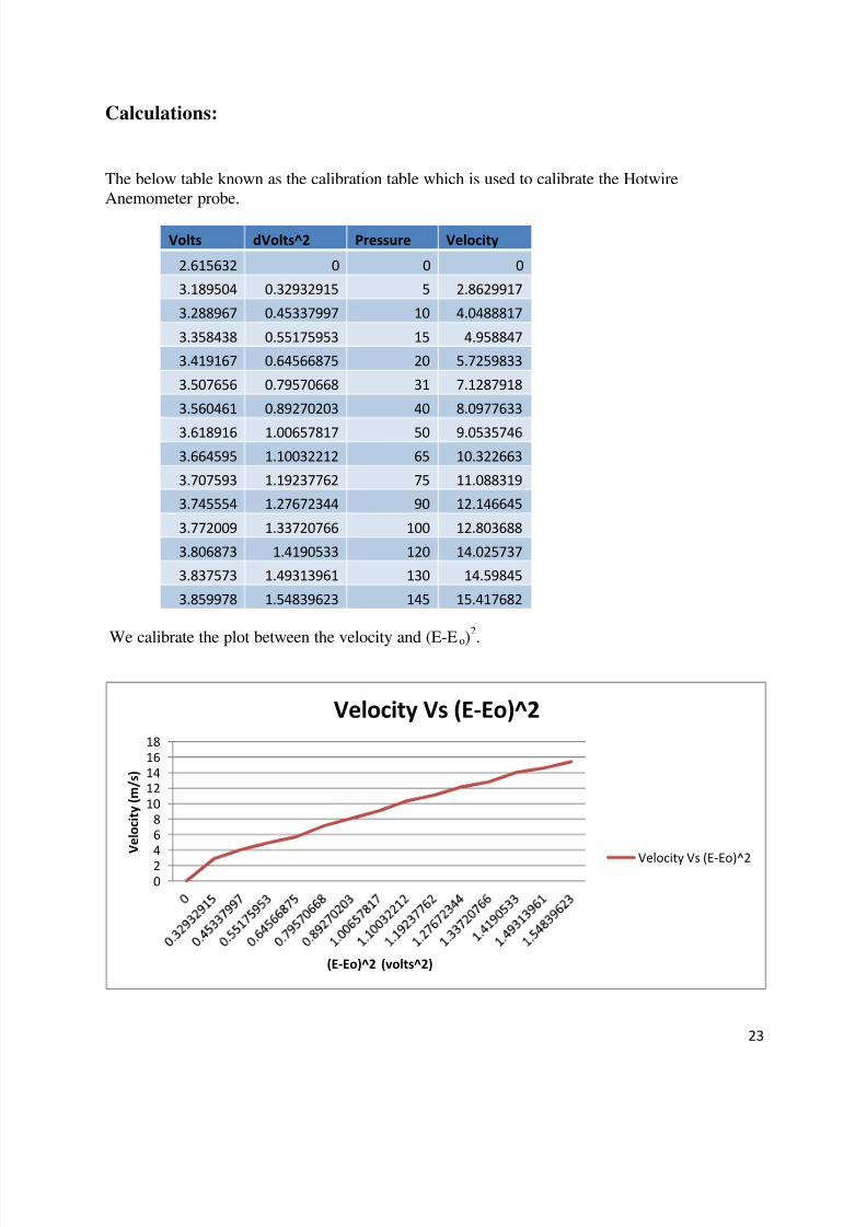
Calculations:
The below table known as the calibration table which is used to calibrate the Hotwire
Anemometer probe.
Volts dVolts^2 Pressure Velocity
2.615632 0 0 0
3.189504 0.32932915 5 2.8629917
3.288967 0.45337997 10 4.0488817
3.358438 0.55175953 15 4.958847
3.419167 0.64566875 20 5.7259833
3.507656 0.79570668 31 7.1287918
3.560461 0.89270203 40 8.0977633
3.618916 1.00657817 50 9.0535746
3.664595 1.10032212 65 10.322663
3.707593 1.19237762 75 11.088319
3.745554 1.27672344 90 12.146645
3.772009 1.33720766 100 12.803688
3.806873 1.4190533 120 14.025737
3.837573 1.49313961 130 14.59845
3.859978 1.54839623 145 15.417682
We calibrate the plot between the velocity and (E-Eo)
2
.
0
2
4
6
8
10
12
14
16
18
V e l o c i t y ( m / s )
(E-Eo)^2 (volts^2)
Velocity Vs (E-Eo)^2
Velocity Vs (E-Eo)^2

8/3/2019 Vortex_Khwaja Saleem a
http://slidepdf.com/reader/full/vortexkhwaja-saleem-a 24/30
24
Given that:
Diameter of the Cylinder, d = 15.0mm
Free Stream Velocity, U0 = 10.0 m/s
Strouhal Number, St = 0.2
• Verifying weather the flow is laminar or turbulent as per Reynolds Number
Reynolds number:
Re =ρ
µ ……………………………………………………[1]
Where ρ = Fluid Density (Kg/m3)
Uo = Free Stream Velocity (m/s)
d = Diameter of the cylinder (m)
µ = Dynamic Viscosity of the Fluid (N.s/m2)
Using standard temperature and pressure of 20°C
ρ = 1.2047 kg/m3
µ = 1.8205E-5N.s/m2
Re =.∗∗.
.= 9128
As explained earlier shedding occurs in the range between 102<Re<107, with an average Strouhal
Number ~ 0.21.
Hence, the fluid flow of the experiment is a turbulent flow.
• Calculating Strouhal Number
Strouhal Number in terms of Reynolds number (Re) is given by:
St = 0.198 (1 – . )
i.e, 0.198 (1 –.) = 0.2
St = 0.2
Hence the calculated Strouhal number is same as the estimated experimental data.

8/3/2019 Vortex_Khwaja Saleem a
http://slidepdf.com/reader/full/vortexkhwaja-saleem-a 25/30
25
• Estimating the frequency of Vortex Shedding
Where St =
………………………………………………….[2]
f= Vortex Shedding Frequency (Hz)
d = Diameter of the Cylinder (m)
U0 = Free Stream Velocity (m/s)
f =∗.. = 133.33Hz
Maximum frequency due to two vortices 2f = 2/t
i.e., f = 2 * (133.33)
Max Frequency = 266.66Hz
• Calculating Ideal Sampling rate:
Ideal sampling rate is obtained by multiplying max frequency by 2.5 according to Nyquist theory
Ideal sampling rate: 2.5 * Max Fre = 2.5 * 266.66
666.65
Adjusted Ideal sampling frequency = 700Hz
a) Calculating the number of ideal sampling data:
Number of sample data = 2n
For n = 10, the number of sample data
i.e., 210
= 1024

8/3/2019 Vortex_Khwaja Saleem a
http://slidepdf.com/reader/full/vortexkhwaja-saleem-a 26/30
26
b) Calculating Mean Velocity:
=
……………………………………………………..[3]
= Mean Velocity (m/s)
Ui = Velocity of Each Individual Data (m/s)
n = Number of Sample
i.e., =
(.⋯.)
= 8.174 m/s
c) Root Mean Square (RMS):
RMS value is obtained by using 0mmset1024700.csv file and is executed is the Matlab script.
RMS (Root-Mean-Square) value of the Fluctuation Component of Velocity:
………………………………… [4]
RMS = ((.)⋯(.))
− (8.174)2
RMS (ú) = 1.8724 m/s
The Relative Turbulence Intensity (RTI):
RTI =(ú)
× 100% ……………………………………………..[5]
=.. * 100= 22.90%
RTI = 22.90%

8/3/2019 Vortex_Khwaja Saleem a
http://slidepdf.com/reader/full/vortexkhwaja-saleem-a 27/30
27
Discussion of Results:
In the first phase of results, where we find the optimum, over and under sampling rate we
can make the following observations. When we consider the optimum sampling rate i.e.
700 Hz with 1024 samples per second the data we receive from the plot is sufficiently
enough. And we can obtain clear and correct results. Both f and 2f are present in von
Karman Vortex Street. In case of over sampling rate we acquire data greater than the
optimum sampling rate that is 1024 Hz with 2048 samples per second. In this case the f
and 2f values are clear but there are other energy sources within the plot which disturbs
the plot and unwanted memory is lost. Though there is always a high quality result
available for a over sampling rate.
The under sampling case is rather different from the earlier two. The sampling rate is 350
Hz with 512 samples per second. The data acquired from the plot is not sufficient to
predict the f and 2f frequencies in the spectrum. Hence under sampling gives a low
frequency output.
When we consider the frequency spectra at any 3 position ex. At 0mm, 50mm, and
100mm and their respectively graphs shows different results. The 0mm grapg shows the
highest fluctuation velocity when compared to the other two. Similarly when we consider
the velocity histogram the plot of 0mm is wider when compared to 50mm or 100mm.this
all depends on the position of the hotwire anemometer. The graph also show a wider
RMS range due to the velocity fluctuation compared to smaller RMS of the other two
positions.
Consider the velocity probability distribution across the wake, due to the turbulent natureof the flow the velocities that are occurring in the wake flow are more. As we go down
the wake the range gets narrow to few velocities which is around 10m/s.
The RMS velocity is measure of the turbulent in the flow, so we can see that as we go
down across the wake the RMS component reduces and goes almost to unity. The RTI
also reduces across the wake.
Velocity histories graph indicates the variation in the RMS and RTI values as well as the
mean velocity. The RMS and RTI variations are considerable criteria to investigate the
nature of the flow. Decreasing in both the RMS and RTI produces more laminarflow.Moreover, the optimum sampling mode has the most obvious velocity history
compared to two other sampling modes.
8/3/2019 Vortex_Khwaja Saleem a
http://slidepdf.com/reader/full/vortexkhwaja-saleem-a 28/30
28
Conclusions:
• We obtain the optimum sampling rate i.e. 700Hz with 1024 samples per second. This is
achieved with the help of Nyquist sampling theory and also acquired the data from vonKarman Vortex street produced by circular cylinder.
• The position of the probe effects the frequency spectra graph and on the PDF. As increasein distance of probe from the centre of the test section decrease the PDF.
• The RTI and RMS are very important to find the nature of the flow.
• Magnitude of energy at vortex shedding reduces across the wake.
Acknowledgement:
My sincere thanks to Mr. Dennis Cooper and Dr. Andrew Kennaugh who taught and guided
me to carry out this experiment.
References:
Cooper.D., 2011, Vortex shedding from a cylinder and data acquisition, MACE61078
Research methods. The University of Manchester.
Cooper.D., 2011, Lecture #- Data analysis, Research methods, The University of
Manchester.
Von Karman vortex street image from:
http://panoramix.ift.uni.wroc.pl/~maq/eng/cfdthesis.php
White F.M., Fluid Mechanics, McGraw-Hill,1999.

8/3/2019 Vortex_Khwaja Saleem a
http://slidepdf.com/reader/full/vortexkhwaja-saleem-a 29/30
29
Appendix A
%optimum sampling at 700 Hz
rawdata_opti=importdata('0mmset1024700.csv');
velocity_opti=rawdata_opti(:,4);fft_opti= fft_opti= fft(velocity_opti,1024);
magnitude_opti=abs(fft_opti(1:513,:));
frequency_opti=[0:1:512].*(700/1024);
subplot(3,1,1),plot(frequency_opti,magnitude_opti);
xlabel('frequency');
ylabel('magnitude');
title('optimum sampling at 700 Hz');
axis([0 400 0 350]);
%over sampling rate at 1400 Hz
rawdata_over=importdata('0mmset10241400.csv');velocity_over=rawdata_over(:,4);
fft_over= fft(velocity_over,1024);
magnitude_over=abs(fft_over(1:513,:));
frequency_over=[0:1:512].*(700/1024);
subplot(3,1,2),plot(frequency_over,magnitude_over);
xlabel('frequency');
ylabel('magnitude');
title('over sampling at 1400 Hz');
axis([0 400 0 350]);
%under sampling rate at 350 Hz
rawdata_under=importdata('0mmset512350.csv');
velocity_under=rawdata_under(:,4);
fft_under= fft(velocity_under,512);
magnitude_under=abs(fft_under(1:257,:));
frequency_under=[0:1:256].*(350/512);
subplot(3,1,3),plot(frequency_under,magnitude_under);
xlabel('frequency');
ylabel('magnitude');
title('under sampling at 350 Hz');
axis([0 200 0 350]);
%frequency spectra at centre
rawdata_opti=importdata('0mmset1024700.csv');
velocity_opti=rawdata_opti(:,4);
fft_opti= fft(velocity_opti,1024);
magnitude_opti=abs(fft_opti(1:513,:));
frequency_opti=[0:1:512].*(700/1024);
subplot(3,4,1),plot(frequency_opti,magnitude_opti);

8/3/2019 Vortex_Khwaja Saleem a
http://slidepdf.com/reader/full/vortexkhwaja-saleem-a 30/30
xlabel('frequency (Hz)');
ylabel('magnitude (Hz/W^2)');
title('Frequency spectra at centre of cylinder');
axis([0 400 0 350]);
%histogram for velocities at the center
rawdata_0mm= importdata('0mmset1024700.csv');
u_0mm=rawdata_0mm(:,4);
bins=[0:0.2:20]';
subplot(4,3,1),hist(u_0mm,bins);
title('histogram for velocities at centre');
xlabel('velocity bins');
ylabel('frequency of occurance of velocity');
%%%%%%%%mean velocity and rms velocities%%%%%%%%%%
rawdata_0mm=importdata('0mmset1024700.csv');
u_0mm=rawdata_0mm(:,4);
u_mean_0mm=mean(u_0mm);
u_rms_0mm=std(u_0mm);
Umean= [ u_mean_0mm]';
Urms= [u_rms_0mm]';
wake= [ 0:10:100]';
RTI = (Urms./Umean)*(100);
plot(wake,Umean,'--');
hold on
ploy(wake,Urms);
xlabel('distance from centre in mm')ylabel('velocity (m/s)')
axis([0 100 -1 15])
legend('Umean across the wake','Urms across the wake')
title('Umean and Urms profile across the wake')
%%%%%%%%%relative turbulence intensity across the wake%%%%%%%%%%
rawdata_0mm=importdata('0mmset1024700.csv');
u_0mm=rawdata_0mm(:,4);
u_mean_0mm=mean(u_0mm);
u_rms_0mm=std(u_0mm);
Umean= [ u_mean_0mm]';Urms= [u_rms_0mm]';
wake= [ 0:10:100]';
RTI = (Urms./Umean)*(100);
plot(wake,RTI);
xlabel('distance from centre in MM')
ylabel('% of RTI');
title('Relative Turbulence intensity across the wake');