Voronoi Diagrams and Delaunay Triangulations...Voronoi Diagrams and Delaunay Triangulations...
72
Voronoi Diagrams and Delaunay Triangulations Jean-Daniel Boissonnat MPRI, Lecture 1, September 20, 2012 Computational Geometric Learning Voronoi Diagrams and Delaunay Triangulations
Transcript of Voronoi Diagrams and Delaunay Triangulations...Voronoi Diagrams and Delaunay Triangulations...

Voronoi Diagrams and DelaunayTriangulations
Jean-Daniel Boissonnat
MPRI, Lecture 1, September 20, 2012
Computational Geometric Learning Voronoi Diagrams and Delaunay Triangulations
Outline
I Euclidean Voronoi diagramsI Delaunay triangulationsI Convex hulls
Computational Geometric Learning Voronoi Diagrams and Delaunay Triangulations
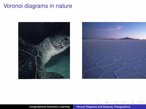
Voronoi diagrams in nature
Computational Geometric Learning Voronoi Diagrams and Delaunay Triangulations
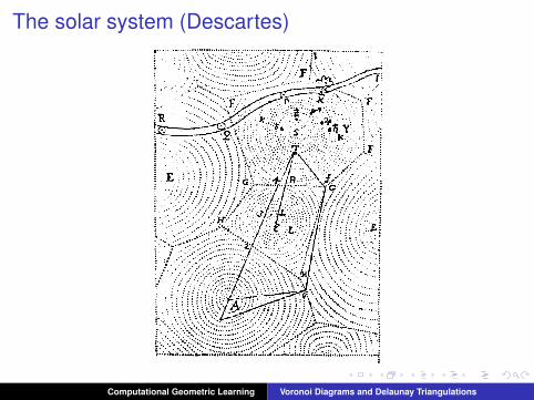
The solar system (Descartes)
Computational Geometric Learning Voronoi Diagrams and Delaunay Triangulations
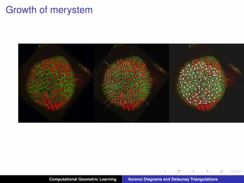
Growth of merystem
Computational Geometric Learning Voronoi Diagrams and Delaunay Triangulations
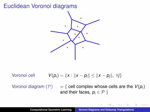
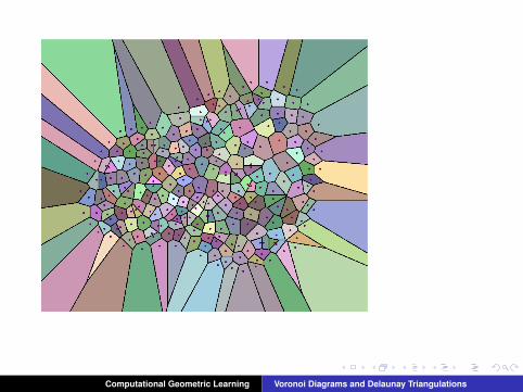
Euclidean Voronoi diagrams
Voronoi cell V (pi) = x : ‖x − pi‖ ≤ ‖x − pj‖, ∀j
Voronoi diagram (P) = cell complex whose cells are the V (pi)and their faces, pi ∈ P
Computational Geometric Learning Voronoi Diagrams and Delaunay Triangulations
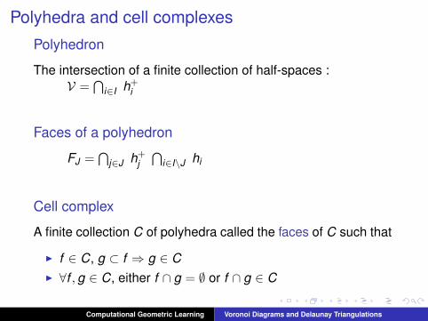
Polyhedra and cell complexes
Polyhedron
The intersection of a finite collection of half-spaces :V =
⋂i∈I h+
i
Faces of a polyhedron
FJ =⋂
j∈J h+j⋂
i∈I\J hi
Cell complex
A finite collection C of polyhedra called the faces of C such that
I f ∈ C, g ⊂ f ⇒ g ∈ CI ∀f ,g ∈ C, either f ∩ g = ∅ or f ∩ g ∈ C
Computational Geometric Learning Voronoi Diagrams and Delaunay Triangulations
Computational Geometric Learning Voronoi Diagrams and Delaunay Triangulations
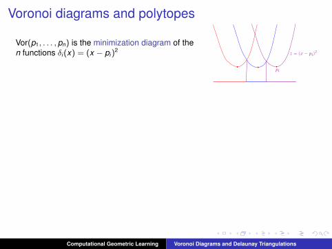
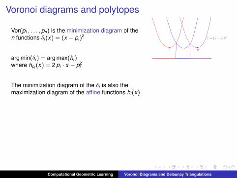
Voronoi diagrams and polytopes
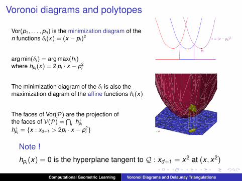
Vor(p1, . . . , pn) is the minimization diagram of then functions δi(x) = (x − pi)
2
arg min(δi) = arg max(hi)where hpi (x) = 2 pi · x − p2
i
The minimization diagram of the δi is also themaximization diagram of the affine functions hi(x)
The faces of Vor(P) are the projection ofthe faces of V(P) =
⋂i h+
pi
h+pi= x : xd+1 > 2pi · x − p2
i
pi
z = (x− pi)2
Note !
hpi (x) = 0 is the hyperplane tangent to Q : xd+1 = x2 at (x , x2)
Computational Geometric Learning Voronoi Diagrams and Delaunay Triangulations
Voronoi diagrams and polytopes
Vor(p1, . . . , pn) is the minimization diagram of then functions δi(x) = (x − pi)
2
arg min(δi) = arg max(hi)where hpi (x) = 2 pi · x − p2
i
The minimization diagram of the δi is also themaximization diagram of the affine functions hi(x)
The faces of Vor(P) are the projection ofthe faces of V(P) =
⋂i h+
pi
h+pi= x : xd+1 > 2pi · x − p2
i
pi
z = (x− pi)2
Note !
hpi (x) = 0 is the hyperplane tangent to Q : xd+1 = x2 at (x , x2)
Computational Geometric Learning Voronoi Diagrams and Delaunay Triangulations
Voronoi diagrams and polytopes
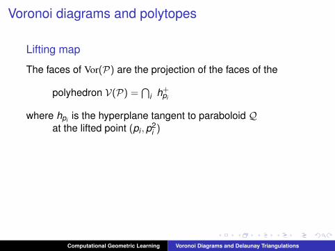
Lifting map
The faces of Vor(P) are the projection of the faces of the
polyhedron V(P) =⋂
i h+pi
where hpi is the hyperplane tangent to paraboloid Qat the lifted point (pi ,p2
i )
Corollaries
I The size of Vor(P) is the same as the size of V(P)
I Computing Vor(P) reduces to computing V(P)
Computational Geometric Learning Voronoi Diagrams and Delaunay Triangulations

Voronoi diagrams and polytopes
Lifting map
The faces of Vor(P) are the projection of the faces of the
polyhedron V(P) =⋂
i h+pi
where hpi is the hyperplane tangent to paraboloid Qat the lifted point (pi ,p2
i )
Corollaries
I The size of Vor(P) is the same as the size of V(P)
I Computing Vor(P) reduces to computing V(P)
Computational Geometric Learning Voronoi Diagrams and Delaunay Triangulations

Delaunay Triangulations
Computational Geometric Learning Voronoi Diagrams and Delaunay Triangulations
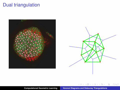
Dual triangulation
Computational Geometric Learning Voronoi Diagrams and Delaunay Triangulations
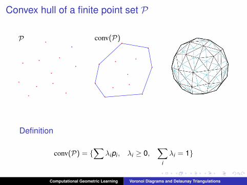
Convex hull of a finite point set P
P conv(P)
Definition
conv(P) = ∑
λipi , λi ≥ 0,∑
i
λi = 1
Computational Geometric Learning Voronoi Diagrams and Delaunay Triangulations
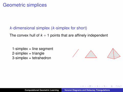
Geometric simplices
k -dimensional simplex (k -simplex for short)
The convex hull of k + 1 points that are affinely independent
1-simplex = line segment2-simplex = triangle3-simplex = tetrahedron
Computational Geometric Learning Voronoi Diagrams and Delaunay Triangulations
Geometric simplicial complexes
Definition
A finite collection of simplices C called the faces of C such that
I ∀f ∈ C, f is a simplexI f ∈ C, f ⊂ g ⇒ g ∈ CI ∀f ,g ∈ C, either f ∩ g = ∅ or f ∩ g ∈ C
The dimension of the complex is the max dimension of itssimplices
Computational Geometric Learning Voronoi Diagrams and Delaunay Triangulations
Abstract simplicial complexes
Given a finite set of points P (not necessarily from a Euclideanspace) a subset C = σ1, ..., σm is a simplicial complex if
1. ∀i , σi ⊂ P2. ∀i , all the subsets of σi are in C3. ∀i , j , σi ∩ σj ∈ C
Theorem
Any simplicial complex of dimension k can be embedded inR2k+1
Computational Geometric Learning Voronoi Diagrams and Delaunay Triangulations
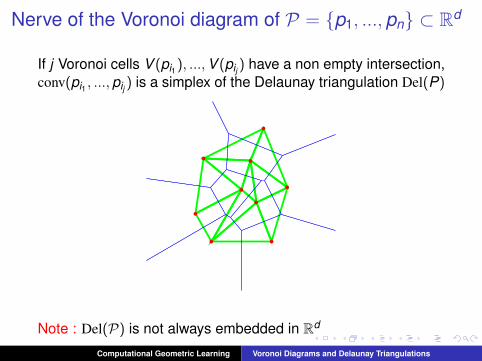
Nerve of the Voronoi diagram of P = p1, ...,pn ⊂ Rd
If j Voronoi cells V (pi1), ...,V (pij ) have a non empty intersection,conv(pi1 , ...,pij ) is a simplex of the Delaunay triangulation Del(P)
Note : Del(P) is not always embedded in Rd
Computational Geometric Learning Voronoi Diagrams and Delaunay Triangulations
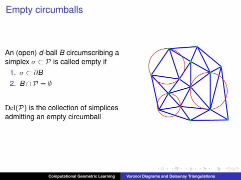
Empty circumballs
An (open) d-ball B circumscribing asimplex σ ⊂ P is called empty if
1. σ ⊂ ∂B2. B ∩ P = ∅
Del(P) is the collection of simplicesadmitting an empty circumball
Computational Geometric Learning Voronoi Diagrams and Delaunay Triangulations
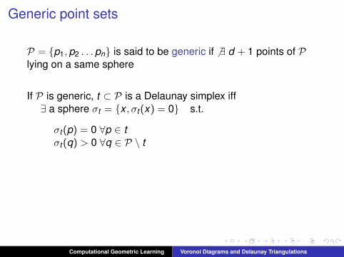
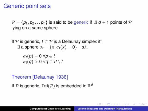
Generic point sets
P = p1,p2 . . . pn is said to be generic if 6 ∃ d + 1 points of Plying on a same sphere
If P is generic, t ⊂ P is a Delaunay simplex iff∃ a sphere σt = x , σt (x) = 0 s.t.
σt (p) = 0 ∀p ∈ tσt (q) > 0 ∀q ∈ P \ t
Theorem [Delaunay 1936]
If P is generic, Del(P) is embedded in Rd
Computational Geometric Learning Voronoi Diagrams and Delaunay Triangulations
Proof of Delaunay’s theorem
σ
h(σ)
P
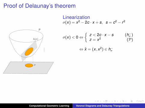
Linearizationσ(x) = x2 − 2c · x + s, s = c2 − r2
σ(x) < 0⇔
z < 2c · x − s (h−σ )z = x2 (P)
⇔ x = (x , x2) ∈ h−σ
Proof of Delaunay’s th.t a simplex, σt its circumscribing sphere
t ∈ Del(P)⇔ ∀i , pi ∈ h+σt
⇔ t is a face of conv−(P)
Del(P) = proj(conv−(P))
Computational Geometric Learning Voronoi Diagrams and Delaunay Triangulations
Proof of Delaunay’s theorem
σ
h(σ)
P
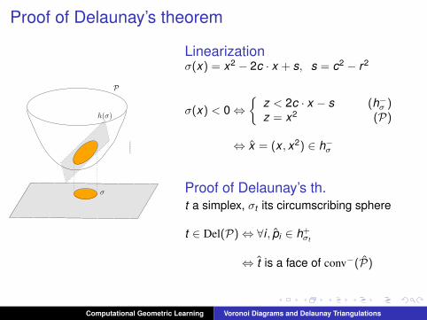
Linearizationσ(x) = x2 − 2c · x + s, s = c2 − r2
σ(x) < 0⇔
z < 2c · x − s (h−σ )z = x2 (P)
⇔ x = (x , x2) ∈ h−σ
Proof of Delaunay’s th.t a simplex, σt its circumscribing sphere
t ∈ Del(P)⇔ ∀i , pi ∈ h+σt
⇔ t is a face of conv−(P)
Del(P) = proj(conv−(P))
Computational Geometric Learning Voronoi Diagrams and Delaunay Triangulations
Proof of Delaunay’s theorem
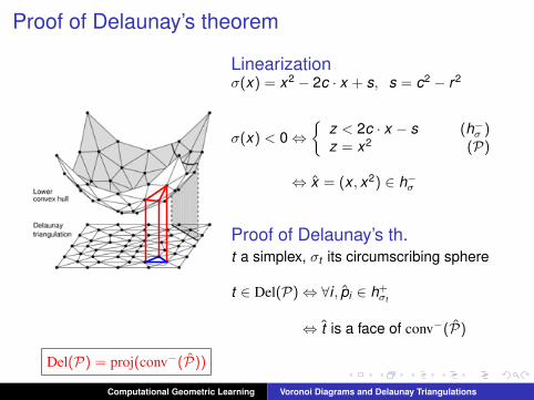
Linearizationσ(x) = x2 − 2c · x + s, s = c2 − r2
σ(x) < 0⇔
z < 2c · x − s (h−σ )z = x2 (P)
⇔ x = (x , x2) ∈ h−σ
Proof of Delaunay’s th.t a simplex, σt its circumscribing sphere
t ∈ Del(P)⇔ ∀i , pi ∈ h+σt
⇔ t is a face of conv−(P)
Del(P) = proj(conv−(P))
Computational Geometric Learning Voronoi Diagrams and Delaunay Triangulations
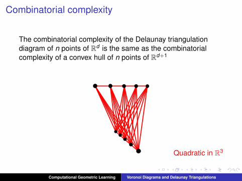
Combinatorial complexity
The combinatorial complexity of the Delaunay triangulationdiagram of n points of Rd is the same as the combinatorialcomplexity of a convex hull of n points of Rd+1
Quadratic in R3
Computational Geometric Learning Voronoi Diagrams and Delaunay Triangulations
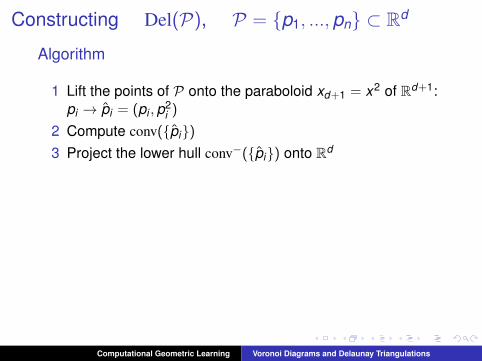
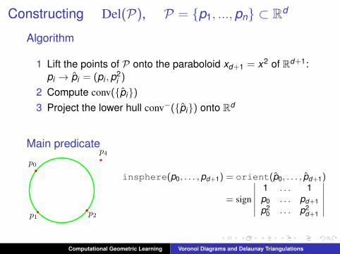
Constructing Del(P), P = p1, ...,pn ⊂ Rd
Algorithm
1 Lift the points of P onto the paraboloid xd+1 = x2 of Rd+1:pi → pi = (pi ,p2
i )
2 Compute conv(pi)3 Project the lower hull conv−(pi) onto Rd
Main predicate
p0
p1 p2
p4
insphere(p0, . . . ,pd+1) = orient(p0, . . . , pd+1)
= sign
∣∣∣∣∣∣1 . . . 1p0 . . . pd+1p2
0 . . . p2d+1
∣∣∣∣∣∣
Computational Geometric Learning Voronoi Diagrams and Delaunay Triangulations
Constructing Del(P), P = p1, ...,pn ⊂ Rd
Algorithm
1 Lift the points of P onto the paraboloid xd+1 = x2 of Rd+1:pi → pi = (pi ,p2
i )
2 Compute conv(pi)3 Project the lower hull conv−(pi) onto Rd
Main predicate
p0
p1 p2
p4
insphere(p0, . . . ,pd+1) = orient(p0, . . . , pd+1)
= sign
∣∣∣∣∣∣1 . . . 1p0 . . . pd+1p2
0 . . . p2d+1
∣∣∣∣∣∣Computational Geometric Learning Voronoi Diagrams and Delaunay Triangulations
Convex Hulls
Computational Geometric Learning Voronoi Diagrams and Delaunay Triangulations
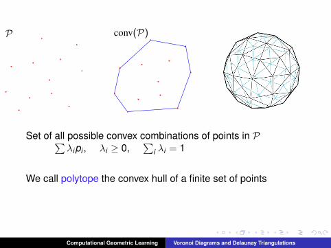
P conv(P)
Set of all possible convex combinations of points in P∑λipi , λi ≥ 0,
∑i λi = 1
We call polytope the convex hull of a finite set of points
Computational Geometric Learning Voronoi Diagrams and Delaunay Triangulations
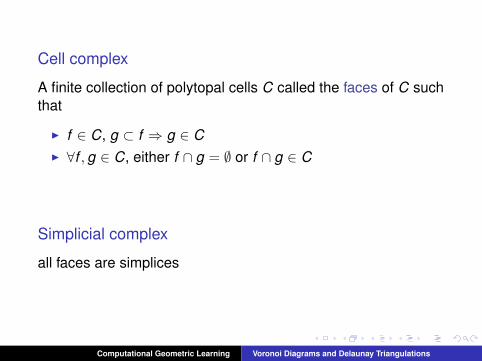
Cell complex
A finite collection of polytopal cells C called the faces of C suchthat
I f ∈ C, g ⊂ f ⇒ g ∈ CI ∀f ,g ∈ C, either f ∩ g = ∅ or f ∩ g ∈ C
Simplicial complex
all faces are simplices
Computational Geometric Learning Voronoi Diagrams and Delaunay Triangulations
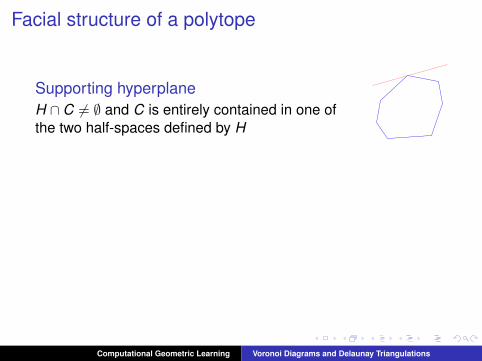
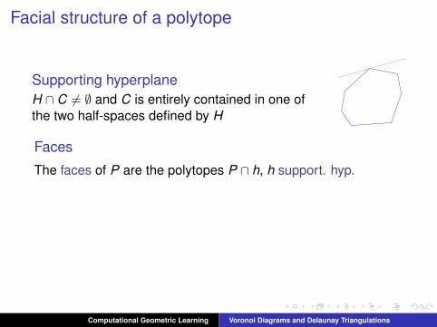
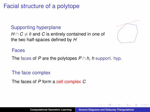
Facial structure of a polytope
Supporting hyperplaneH ∩ C 6= ∅ and C is entirely contained in one ofthe two half-spaces defined by H
Faces
The faces of P are the polytopes P ∩ h, h support. hyp.
The face complex
The faces of P form a cell complex C
Computational Geometric Learning Voronoi Diagrams and Delaunay Triangulations
General position
General position
A point set P is said to be in general position iff no subset ofk + 2 points lie in a k -flat
Boundary complex
If P is in general position, all the faces of conv(P) are simplices
The boundary of conv(P) is a simplicial complex
Computational Geometric Learning Voronoi Diagrams and Delaunay Triangulations
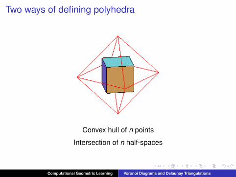
Two ways of defining polyhedra
Convex hull of n points
Intersection of n half-spaces
Computational Geometric Learning Voronoi Diagrams and Delaunay Triangulations
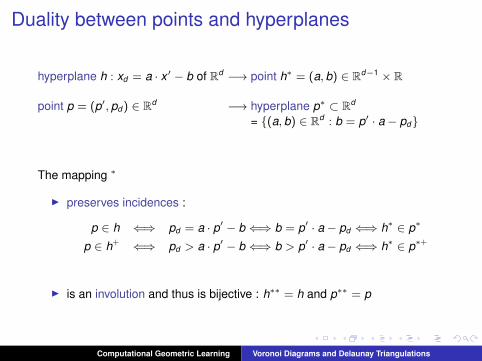
Duality between points and hyperplanes
hyperplane h : xd = a · x ′ − b of Rd −→ point h∗ = (a, b) ∈ Rd−1 × R
point p = (p′, pd) ∈ Rd −→ hyperplane p∗ ⊂ Rd
= (a, b) ∈ Rd : b = p′ · a− pd
The mapping ∗
I preserves incidences :
p ∈ h ⇐⇒ pd = a · p′ − b ⇐⇒ b = p′ · a− pd ⇐⇒ h∗ ∈ p∗
p ∈ h+ ⇐⇒ pd > a · p′ − b ⇐⇒ b > p′ · a− pd ⇐⇒ h∗ ∈ p∗+
I is an involution and thus is bijective : h∗∗ = h and p∗∗ = p
Computational Geometric Learning Voronoi Diagrams and Delaunay Triangulations
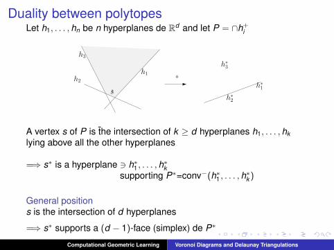
Duality between polytopesLet h1, . . . ,hn be n hyperplanes de Rd and let P = ∩h+
i
ss
h1h2 *
h3
h∗3
h∗2
h∗1
A vertex s of P is the intersection of k ≥ d hyperplanes h1, . . . ,hklying above all the other hyperplanes
=⇒ s∗ is a hyperplane 3 h∗1 , . . . ,h∗k
supporting P∗=conv−(h∗1 , . . . ,h∗k )
General positions is the intersection of d hyperplanes
=⇒ s∗ supports a (d − 1)-face (simplex) de P∗
Computational Geometric Learning Voronoi Diagrams and Delaunay Triangulations
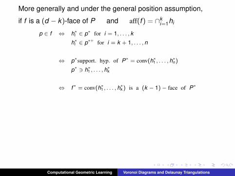
More generally and under the general position assumption,
if f is a (d − k)-face of P and aff(f ) = ∩ki=1hi
p ∈ f ⇔ h∗i ∈ p∗ for i = 1, . . . , k
h∗i ∈ p∗+ for i = k + 1, . . . , n
⇔ p∗support. hyp. of P∗ = conv(h∗1 , . . . , h∗n )
p∗ 3 h∗1 , . . . , h∗k
⇔ f ∗ = conv(h∗1 , . . . , h∗k ) is a (k − 1)− face of P∗
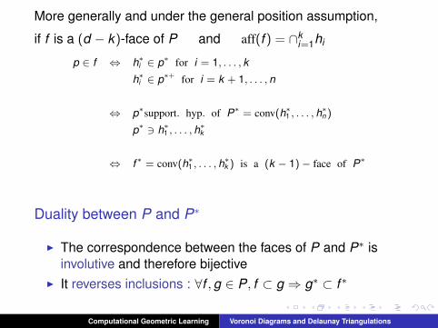
Duality between P and P∗
I The correspondence between the faces of P and P∗ isinvolutive and therefore bijective
I It reverses inclusions : ∀f ,g ∈ P, f ⊂ g ⇒ g∗ ⊂ f ∗
Computational Geometric Learning Voronoi Diagrams and Delaunay Triangulations
More generally and under the general position assumption,
if f is a (d − k)-face of P and aff(f ) = ∩ki=1hi
p ∈ f ⇔ h∗i ∈ p∗ for i = 1, . . . , k
h∗i ∈ p∗+ for i = k + 1, . . . , n
⇔ p∗support. hyp. of P∗ = conv(h∗1 , . . . , h∗n )
p∗ 3 h∗1 , . . . , h∗k
⇔ f ∗ = conv(h∗1 , . . . , h∗k ) is a (k − 1)− face of P∗
Duality between P and P∗
I The correspondence between the faces of P and P∗ isinvolutive and therefore bijective
I It reverses inclusions : ∀f ,g ∈ P, f ⊂ g ⇒ g∗ ⊂ f ∗
Computational Geometric Learning Voronoi Diagrams and Delaunay Triangulations
Algorithmic consequences
I Computing the intersection of n upper half-spaces or thelower convex hull of n points are equivalent problems
I Depending on the application, the primal or the dual settingmay be more appropriate
Computational Geometric Learning Voronoi Diagrams and Delaunay Triangulations
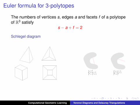
Euler formula for 3-polytopes
The numbers of vertices s, edges a and facets f of a polytopeof R3 satisfy
s − a + f = 2
Schlegel diagram
s = s′a′ = a + 1f ′ = f + 1
a′ = a + 1f ′ = f
s′ = s + 1
Computational Geometric Learning Voronoi Diagrams and Delaunay Triangulations
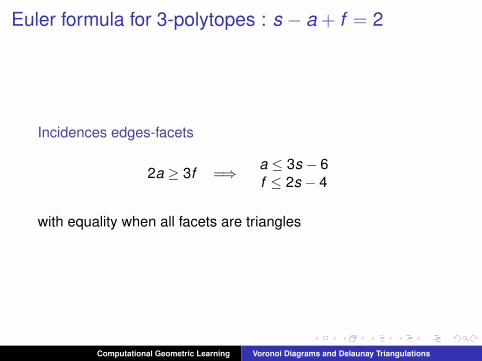
Euler formula for 3-polytopes : s − a + f = 2
Incidences edges-facets
2a ≥ 3f =⇒ a ≤ 3s − 6f ≤ 2s − 4
with equality when all facets are triangles
Computational Geometric Learning Voronoi Diagrams and Delaunay Triangulations
Beyond the 3rd dimensionUpper bound theorem [McMullen 1970]
If P is the intersection of n half-spaces of Rd
nb faces of P = Θ(nb d2 c)
General position
I all vertices of P are incident to d edges (in the worst-case)and have distinct xd
I the convex hull of k < d edges incident to a vertex pis a k -face of P
I any k -face is the intersection of d − k hyperplanesdefining P
Computational Geometric Learning Voronoi Diagrams and Delaunay Triangulations
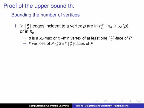
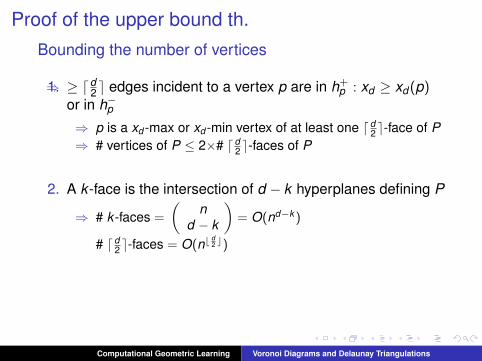
Proof of the upper bound th.Bounding the number of vertices
1. ≥ dd2 e edges incident to a vertex p are in h+
p : xd ≥ xd (p)or in h−p⇒ p is a xd -max or xd -min vertex of at least one d d
2 e-face of P⇒ # vertices of P ≤ 2×# d d
2 e-faces of P
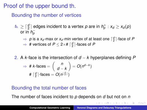
2. A k -face is the intersection of d − k hyperplanes defining P
⇒ # k -faces =
(n
d − k
)= O(nd−k )
# d d2 e-faces = O(nb
d2 c)
Bounding the total number of faces
The number of faces incident to p depends on d but not on n
Computational Geometric Learning Voronoi Diagrams and Delaunay Triangulations
Proof of the upper bound th.Bounding the number of vertices
⇒1. ≥ dd2 e edges incident to a vertex p are in h+
p : xd ≥ xd (p)or in h−p⇒ p is a xd -max or xd -min vertex of at least one d d
2 e-face of P⇒ # vertices of P ≤ 2×# d d
2 e-faces of P
2. A k -face is the intersection of d − k hyperplanes defining P
⇒ # k -faces =
(n
d − k
)= O(nd−k )
# d d2 e-faces = O(nb
d2 c)
Bounding the total number of faces
The number of faces incident to p depends on d but not on n
Computational Geometric Learning Voronoi Diagrams and Delaunay Triangulations
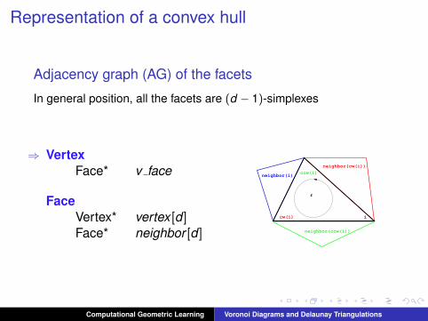
Representation of a convex hull
Adjacency graph (AG) of the facets
In general position, all the facets are (d − 1)-simplexes
⇒ VertexFace* v face
FaceVertex* vertex [d ]Face* neighbor [d ]
i
f
neighbor(ccw(i))
cw(i)
neighbor(i) ccw(i)neighbor(cw(i))
Computational Geometric Learning Voronoi Diagrams and Delaunay Triangulations
Incremental algorithm
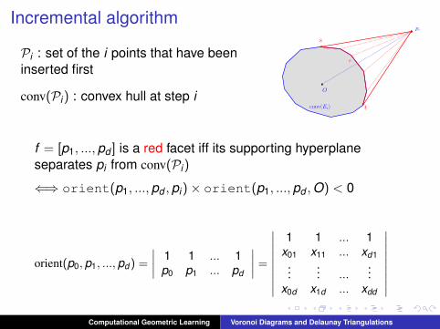
Pi : set of the i points that have beeninserted first
conv(Pi) : convex hull at step iO
pi
conv(Ei)
e
s
t
f = [p1, ...,pd ] is a red facet iff its supporting hyperplaneseparates pi from conv(Pi)
⇐⇒ orient(p1, ...,pd ,pi)× orient(p1, ...,pd ,O) < 0
orient(p0,p1, ...,pd ) =
∣∣∣∣ 1 1 ... 1p0 p1 ... pd
∣∣∣∣ =
∣∣∣∣∣∣∣∣∣1 1 ... 1
x01 x11 ... xd1...
... ......
x0d x1d ... xdd
∣∣∣∣∣∣∣∣∣Computational Geometric Learning Voronoi Diagrams and Delaunay Triangulations
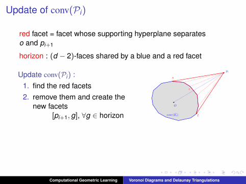
Update of conv(Pi)
red facet = facet whose supporting hyperplane separateso and pi+1
horizon : (d − 2)-faces shared by a blue and a red facet
Update conv(Pi) :1. find the red facets2. remove them and create the
new facets[pi+1,g], ∀g ∈ horizon
O
pi
conv(Ei)
e
s
t
Complexity
proportional to the nb of red facets
Computational Geometric Learning Voronoi Diagrams and Delaunay Triangulations
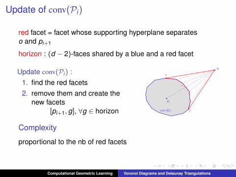
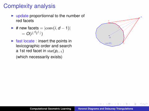
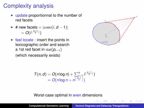
Complexity analysisI update proportionnal to the number of
red facets
I # new facets = |conv(i ,d − 1)|= O(ib
d−12 c)
I fast locate : insert the points inlexicographic order and searcha 1st red facet in star(pi−1)
(which necessarily exists)
O
pi
conv(Ei)
e
s
t
T (n,d) = O(n log n) +∑n
i=1 ibd−1
2 c)
= O(n log n + nb d+12 c)
Worst-case optimal in even dimensions
Computational Geometric Learning Voronoi Diagrams and Delaunay Triangulations
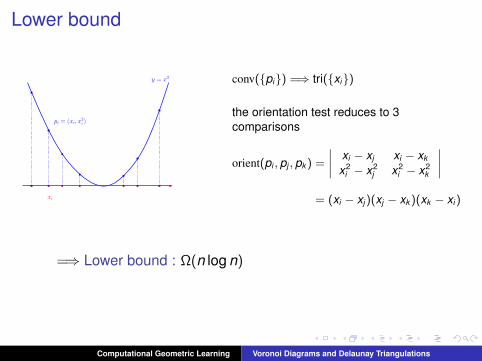
Lower bound
xi
pi = (xi, x2i )
y = x2 conv(pi) =⇒ tri(xi)
the orientation test reduces to 3comparisons
orient(pi , pj , pk ) =
∣∣∣∣ xi − xj xi − xk
x2i − x2
j x2i − x2
k
∣∣∣∣= (xi − xj)(xj − xk )(xk − xi)
=⇒ Lower bound : Ω(n log n)
Computational Geometric Learning Voronoi Diagrams and Delaunay Triangulations
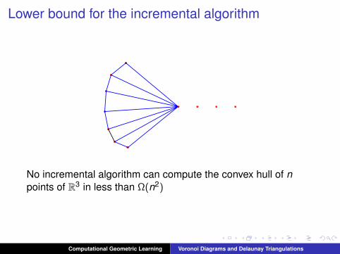
Lower bound for the incremental algorithm
No incremental algorithm can compute the convex hull of npoints of R3 in less than Ω(n2)
Computational Geometric Learning Voronoi Diagrams and Delaunay Triangulations
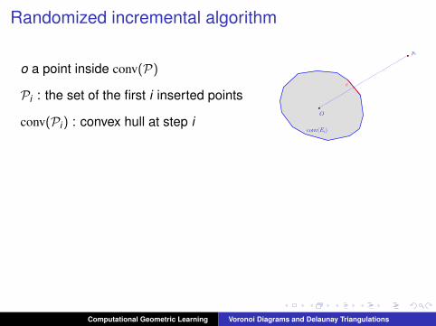
Randomized incremental algorithm
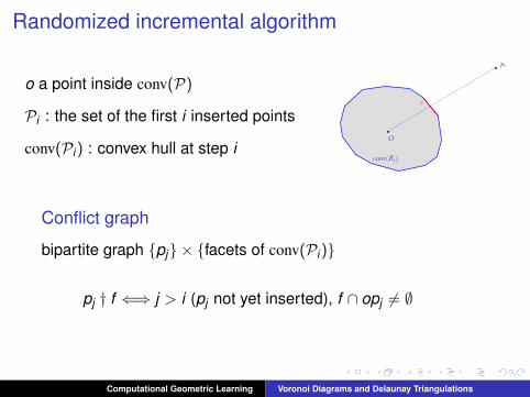
o a point inside conv(P)
Pi : the set of the first i inserted points
conv(Pi) : convex hull at step iO
pi
conv(Ei)
e
Conflict graph
bipartite graph pj × facets of conv(Pi)
pj † f ⇐⇒ j > i (pj not yet inserted), f ∩ opj 6= ∅
Computational Geometric Learning Voronoi Diagrams and Delaunay Triangulations
Randomized incremental algorithm
o a point inside conv(P)
Pi : the set of the first i inserted points
conv(Pi) : convex hull at step iO
pi
conv(Ei)
e
Conflict graph
bipartite graph pj × facets of conv(Pi)
pj † f ⇐⇒ j > i (pj not yet inserted), f ∩ opj 6= ∅
Computational Geometric Learning Voronoi Diagrams and Delaunay Triangulations
Randomized analysis
Hyp. : points are inserted in random order
Notations
R : random sample of size r of P
F (R) = subsets of d points of RF0(R) = elements of F (R) with 0 conflict in R
(i.e. ∈ conv(R))
F1(R) = elements of F (R) with 1 conflict in R
Ci(r ,P) = E(|Fi(R)|)(expectation over all random samples R ⊂ P of size r )
Lemma
C1(r ,P) = C0(r ,P) = O(rb d2 c)
Computational Geometric Learning Voronoi Diagrams and Delaunay Triangulations
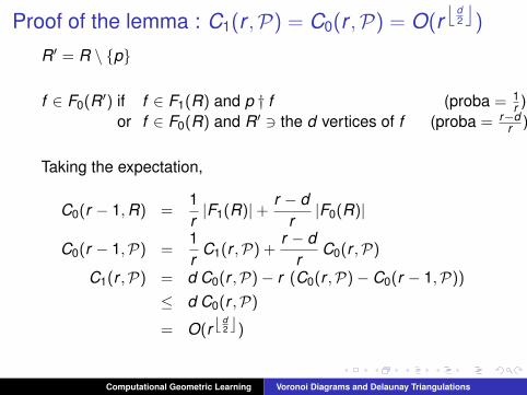
Proof of the lemma : C1(r ,P) = C0(r ,P) = O(rb d2c)
R′ = R \ p
f ∈ F0(R′) if f ∈ F1(R) and p † f (proba = 1r )
or f ∈ F0(R) and R′ 3 the d vertices of f (proba = r−dr )
Taking the expectation,
C0(r − 1,R) =1r|F1(R)|+ r − d
r|F0(R)|
C0(r − 1,P) =1r
C1(r ,P) +r − d
rC0(r ,P)
C1(r ,P) = d C0(r ,P)− r (C0(r ,P)− C0(r − 1,P))
≤ d C0(r ,P)
= O(rb d2 c)
Computational Geometric Learning Voronoi Diagrams and Delaunay Triangulations
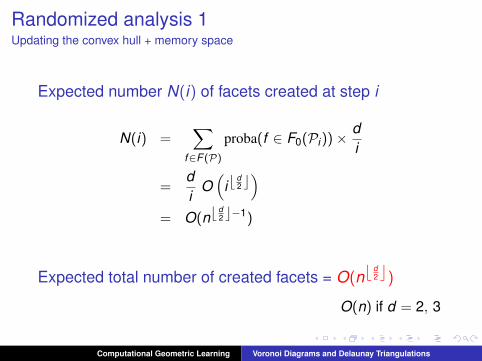
Randomized analysis 1Updating the convex hull + memory space
Expected number N(i) of facets created at step i
N(i) =∑
f∈F (P)
proba(f ∈ F0(Pi))× di
=di
O(
ib d2 c)
= O(nb d2 c−1)
Expected total number of created facets = O(nb d2c)
O(n) if d = 2, 3
Computational Geometric Learning Voronoi Diagrams and Delaunay Triangulations
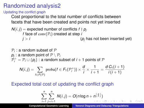
Randomized analysis2Updating the conflict graph
Cost proportional to the total number of conflicts betweenfacets that have been created and points not yet inserted
N(i , j) = expected number of conflicts f † pjf face of conv(Pi ) created at step ij > i (pj has not been inserted yet)
Pi : a random subset of Ppj : a random point of P \ PiP+
i = Pi ∪ pj : a random subset of i + 1 points of P
N(i , j) =∑
f∈F (P)
proba(f ∈ F1(P+i ))× d
i× 1
i + 1=
d C1(i + 1)
i (i + 1)
Expected total cost of updating the conflict graphn∑
i=1
n∑j=i+1
N(i , j) = O(n log n + nb d2 c)
Computational Geometric Learning Voronoi Diagrams and Delaunay Triangulations
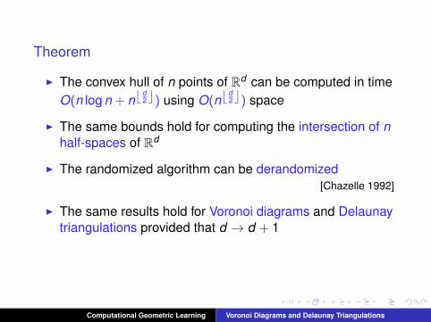
Theorem
I The convex hull of n points of Rd can be computed in timeO(n log n + nb d
2 c) using O(nb d2 c) space
I The same bounds hold for computing the intersection of nhalf-spaces of Rd
I The randomized algorithm can be derandomized[Chazelle 1992]
I The same results hold for Voronoi diagrams and Delaunaytriangulations provided that d → d + 1
Computational Geometric Learning Voronoi Diagrams and Delaunay Triangulations
You know my methods. Apply them !
Sherlock Holmes
Computational Geometric Learning Voronoi Diagrams and Delaunay Triangulations


![Speaker: Tom Gur, 26.4.10 Seminar on Voronoi Diagrams and Delaunay Triangulations Material: [AK] Sections 3.4, 4.1, 4.2, 4.3.1.](https://static.fdocuments.in/doc/165x107/56649d2d5503460f94a037d0/speaker-tom-gur-26410-seminar-on-voronoi-diagrams-and-delaunay-triangulations.jpg)