![Adaptive Cube Tessellation for Topologically Correct ... · Adaptive Cube Tessellation for Topologically Correct Isosurfaces ... [PT90]. This method is ... Tessellation for Topologically](https://static.fdocuments.in/doc/165x107/5adfba127f8b9a5a668ca39b/adaptive-cube-tessellation-for-topologically-correct-cube-tessellation-for-topologically.jpg)
Voronoi diagram: An adaptive spatial tessellation for processes
14
Voronoi diagram: An adaptive spatial tessellation for processes simulation 41 X Voronoi diagram: An adaptive spatial tessellation for processes simulation Leila Hashemi Beni, Mir Abolfazl Mostafavi, Jacynthe Pouliot Laval University Canada 1. Introduction Modelling and simulation of spatial processes is increasingly used for a wide variety of applications including water resources protection and management, meteorological prevision and forest fire monitoring. As an example, an accurate spatial modelling of a hydrological system can assist hydrologists to answer questions such as: "where does ground water come from?", “how does it travel through a complex geological system?" and “how is water pollution behaviour in an aquifer?” It also allows users and decision-makers to better understand, analyze and predict the groundwater behaviour. In this chapter, we briefly present an overview of spatial modelling and simulating of a dynamic continuous process such as a fluid flow. Most of the research in this area is based on the numerical modelling and approximation of the dynamic behaviour of a fluid flow. Dynamic continuous process is typically described by a set of partial differential equations (PDE) and their numerical solution is carried out using a spatial tessellation that covers the domain of interest. An efficient solution of the PDE requires methods that are adaptive in both space and time. The existing numerical methods are applied in either a static manner from the Eulerian point of view, where the equations are solved using a fixed tessellation during a simulation process, or in a dynamic manner from the Lagrangian point of view, where the tessellation moves. Some methods are also based on the mixed Eulerian- Lagrangian point of view. However, our literature review reveals that, unfortunately, these methods are unable to efficiently handle the spatial-dynamic behaviour of phenomenon. Therefore, in this chapter, we investigate spatial tessellation based on Voronoi diagram (VD) and its dual Delaunay tessellation (DT) which is good candidate to deal with dynamics behaviour of fluid flow. Voronoi diagram is a topological data structure that discretizes the dynamic phenomenon to a tessellation adaptive in space and time. 2. Numerical modelling methods In computational fluid dynamics, there are two fundamental approaches to simulate fluid flow: Eulerian and Lagrangian flow formulations (Price, 2005). The former is based on a fixed tessellation while the latter uses a moving tessellation. Eulerian methods offer the advantage of a fixed tessellation that is easier to generate, and they can efficiently handle 3 www.intechopen.com
Transcript of Voronoi diagram: An adaptive spatial tessellation for processes
Voronoi diagram: An adaptive spatial tessellation for processes simulation 41
Voronoi diagram: An adaptive spatial tessellation for processes simulation
Leila Hashemi Beni, Mir Abolfazl Mostafavi, Jacynthe Pouliot
X
Voronoi diagram: An adaptive spatial tessellation for processes simulation
Leila Hashemi Beni, Mir Abolfazl Mostafavi, Jacynthe Pouliot
Laval University Canada
1. Introduction
Modelling and simulation of spatial processes is increasingly used for a wide variety of applications including water resources protection and management, meteorological prevision and forest fire monitoring. As an example, an accurate spatial modelling of a hydrological system can assist hydrologists to answer questions such as: "where does ground water come from?", “how does it travel through a complex geological system?" and “how is water pollution behaviour in an aquifer?” It also allows users and decision-makers to better understand, analyze and predict the groundwater behaviour. In this chapter, we briefly present an overview of spatial modelling and simulating of a dynamic continuous process such as a fluid flow. Most of the research in this area is based on the numerical modelling and approximation of the dynamic behaviour of a fluid flow. Dynamic continuous process is typically described by a set of partial differential equations (PDE) and their numerical solution is carried out using a spatial tessellation that covers the domain of interest. An efficient solution of the PDE requires methods that are adaptive in both space and time. The existing numerical methods are applied in either a static manner from the Eulerian point of view, where the equations are solved using a fixed tessellation during a simulation process, or in a dynamic manner from the Lagrangian point of view, where the tessellation moves. Some methods are also based on the mixed Eulerian-Lagrangian point of view. However, our literature review reveals that, unfortunately, these methods are unable to efficiently handle the spatial-dynamic behaviour of phenomenon. Therefore, in this chapter, we investigate spatial tessellation based on Voronoi diagram (VD) and its dual Delaunay tessellation (DT) which is good candidate to deal with dynamics behaviour of fluid flow. Voronoi diagram is a topological data structure that discretizes the dynamic phenomenon to a tessellation adaptive in space and time.
2. Numerical modelling methods
In computational fluid dynamics, there are two fundamental approaches to simulate fluid flow: Eulerian and Lagrangian flow formulations (Price, 2005). The former is based on a fixed tessellation while the latter uses a moving tessellation. Eulerian methods offer the advantage of a fixed tessellation that is easier to generate, and they can efficiently handle
3
www.intechopen.com
Modeling, Simulation and Optimization – Tolerance and Optimal Control42
dispersion dominated transport problems. Eulerian methods are therefore used for a majority of numerical modelling of fluids flow. However, in these methods, the time step size and the tessellation size have to be selected to ensure realistic solutions and avoid overshoot and undershoot of concentrations. However, since a uniformly fine tessellation is computationally costly, these methods are generally not well suited to handle of moving concentration fronts and advection-dominated and tracking problems. Lagrangian methods model the processes by tracking the changing location, shape and values of particles over space and provide an accurate and efficient solution to advection-dominated problems with steep concentration gradients. For Lagrangian methods, the tessellation movement softens the solution behaviour in time, such that larger time steps can be taken compared to a fixed spatial tessellation (Whitehurst, 1995). However, the connectivity between tessellation elements remains unchanged during simulation, which may cause difficulties such as tessellation tangling and deformation that become especially acute in non-uniform media with multiple sources and complex boundary conditions (Neuman 1984)]. In addition, due to the relative nodal motion, the tessellation used for Lagrangian methods becomes distorted over time and complete re-tessellating is frequently required (Malcevic, 2002). Development of mixed Eulerian-Lagrangian methods has led to the class of arbitrary Lagrangian-Eulerian (ALE) codes (Whitehurst, 1995). These codes reduce tessellation distortion by continuous “remapping” or “reconnecting” of the mesh. Tessellation remapping can be regarded as an Eulerian process, because mass is transported across tessellation cell boundaries. The principle of continual remapping led to the Free- Lagrange method. The difference between the Free-Lagrange and the classical Lagrange methods is that the latter attempt to maintain the initial tessellation connectivity during simulation. The Free-Lagrange method allows updating the tessellation connectivity as part of the problem to be solved. Simulation of free-surface flow and variable-density flow and transport are two examples that are well-suited for dynamic modelling. For example, for a hydrogeological system, the free surface or water table is an imaginary surface below ground where the absolute groundwater pressure is atmospheric. The water table moves and dynamic modelling could be used to track its temporal and spatial evolution by using a moving tessellation that conforms to the motion of the free surface. One complexity of using a moving tessellation is to maintain the tessellation alignment with stratigraphic layers or with geological formations having different hydraulic properties. The tessellation alignment can be maintained by continuously updating physical parameters, such as hydraulic conductivity, porosity, storage coefficient, as the tessellation moves. Density-variable flow and transport is another application well-suited for a moving tessellation. A classical example is given by salt-rock formations, where groundwater may become very rich in salt. Zegeling et al. (1992) applied a moving tessellation to simulate 1D brine transport in porous media. They used a dynamic Lagrangian approach to track the sharp fresh-salt water interface and state that, when high concentrations prevail, fixed tessellation methods are inefficient. Moving tessellations have not been efficiently used in 3D since three-dimensionality adds several complexities for simulations. To minimize the problems, the Lagrangian algorithm presented by Knupp (1996) only moves the upper part of the tessellation and movement is restricted to the vertical direction to avoid tessellation deformation.
To solve the tessellation deformation problem and also to avoid the problems involving fixed time-step methods, we propose a new 3D Free-Lagrangian method based on dynamic 3D Voronoi diagram. Voronoi diagram (VD) and its dual, Delaunay triangulation (DT), have been shown to provide an adequate discretization of the space for fluid flow simulation, ensuring that physically realistic results are obtained. The next section describes the Voronoi and Delaunay tessellation with a brief review of their definitions, structures and relevant spatial properties in the context of spatial modelling and simulation of continuous processes.
3. Voronoi and Delaunay tessellation
Fluid flow is continuous and it is practically impossible to measure it anywhere and anytime. Therefore, this continuous phenomenon must be represented using a set of observations in given locations and time which are usually a set of unconnected points. Each point is defined by its position in 2D or 3D space and its attribute at a given time. Voronoi tessellation for this finite set of points is a division of the simulation space based on nearest neighbor rule where every location in the space is assigned to the closet member in the point set. Formally, let S be a set of points in the d-dimensional Euclidean space, the Voronoi tessellation of S associates to each point Sp a Voronoi cell (element) )(pV such that (Okabe et al. 2000, Edelsbrunner 2001): SqqxpxRxpV d ,)( (1)
where px denotes the Euclidean distance between points x , p . Therefore, a Voronoi
element is defined as the set of points dRx that are at least as close to p as to any other point in S . Therefore, a Voronoi tessellation of S is the collection of all Voronoi elements (Okabe et al. 2000): V(q) ..., V(p),v (2) Voronoi tessellation v covers the domain of interest due to the fact that each point
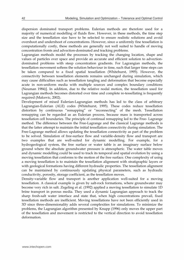
dRx has at least one nearest point in S and it, thus, lies in at least one Voronoi cell. Fig. 1 shows an example of a Voronoi tessellation in 2D and 3D which is a polygonal subdivision of a space consisting of vertices, edges, polygonal faces and cells.
(a) (b) Fig. 1. An example of a Voronoi tessellation a) in 2D, b) in 3D and its components A Delaunay tessellation )(SDT is a collection of d-dimensional simplexes where a simplex is the convex hull of a set of (d + 1) points and no point in S is inside the circum-ball of any
www.intechopen.com
Voronoi diagram: An adaptive spatial tessellation for processes simulation 43
dispersion dominated transport problems. Eulerian methods are therefore used for a majority of numerical modelling of fluids flow. However, in these methods, the time step size and the tessellation size have to be selected to ensure realistic solutions and avoid overshoot and undershoot of concentrations. However, since a uniformly fine tessellation is computationally costly, these methods are generally not well suited to handle of moving concentration fronts and advection-dominated and tracking problems. Lagrangian methods model the processes by tracking the changing location, shape and values of particles over space and provide an accurate and efficient solution to advection-dominated problems with steep concentration gradients. For Lagrangian methods, the tessellation movement softens the solution behaviour in time, such that larger time steps can be taken compared to a fixed spatial tessellation (Whitehurst, 1995). However, the connectivity between tessellation elements remains unchanged during simulation, which may cause difficulties such as tessellation tangling and deformation that become especially acute in non-uniform media with multiple sources and complex boundary conditions (Neuman 1984)]. In addition, due to the relative nodal motion, the tessellation used for Lagrangian methods becomes distorted over time and complete re-tessellating is frequently required (Malcevic, 2002). Development of mixed Eulerian-Lagrangian methods has led to the class of arbitrary Lagrangian-Eulerian (ALE) codes (Whitehurst, 1995). These codes reduce tessellation distortion by continuous “remapping” or “reconnecting” of the mesh. Tessellation remapping can be regarded as an Eulerian process, because mass is transported across tessellation cell boundaries. The principle of continual remapping led to the Free- Lagrange method. The difference between the Free-Lagrange and the classical Lagrange methods is that the latter attempt to maintain the initial tessellation connectivity during simulation. The Free-Lagrange method allows updating the tessellation connectivity as part of the problem to be solved. Simulation of free-surface flow and variable-density flow and transport are two examples that are well-suited for dynamic modelling. For example, for a hydrogeological system, the free surface or water table is an imaginary surface below ground where the absolute groundwater pressure is atmospheric. The water table moves and dynamic modelling could be used to track its temporal and spatial evolution by using a moving tessellation that conforms to the motion of the free surface. One complexity of using a moving tessellation is to maintain the tessellation alignment with stratigraphic layers or with geological formations having different hydraulic properties. The tessellation alignment can be maintained by continuously updating physical parameters, such as hydraulic conductivity, porosity, storage coefficient, as the tessellation moves. Density-variable flow and transport is another application well-suited for a moving tessellation. A classical example is given by salt-rock formations, where groundwater may become very rich in salt. Zegeling et al. (1992) applied a moving tessellation to simulate 1D brine transport in porous media. They used a dynamic Lagrangian approach to track the sharp fresh-salt water interface and state that, when high concentrations prevail, fixed tessellation methods are inefficient. Moving tessellations have not been efficiently used in 3D since three-dimensionality adds several complexities for simulations. To minimize the problems, the Lagrangian algorithm presented by Knupp (1996) only moves the upper part of the tessellation and movement is restricted to the vertical direction to avoid tessellation deformation.
To solve the tessellation deformation problem and also to avoid the problems involving fixed time-step methods, we propose a new 3D Free-Lagrangian method based on dynamic 3D Voronoi diagram. Voronoi diagram (VD) and its dual, Delaunay triangulation (DT), have been shown to provide an adequate discretization of the space for fluid flow simulation, ensuring that physically realistic results are obtained. The next section describes the Voronoi and Delaunay tessellation with a brief review of their definitions, structures and relevant spatial properties in the context of spatial modelling and simulation of continuous processes.
3. Voronoi and Delaunay tessellation
Fluid flow is continuous and it is practically impossible to measure it anywhere and anytime. Therefore, this continuous phenomenon must be represented using a set of observations in given locations and time which are usually a set of unconnected points. Each point is defined by its position in 2D or 3D space and its attribute at a given time. Voronoi tessellation for this finite set of points is a division of the simulation space based on nearest neighbor rule where every location in the space is assigned to the closet member in the point set. Formally, let S be a set of points in the d-dimensional Euclidean space, the Voronoi tessellation of S associates to each point Sp a Voronoi cell (element) )(pV such that (Okabe et al. 2000, Edelsbrunner 2001): SqqxpxRxpV d ,)( (1)
where px denotes the Euclidean distance between points x , p . Therefore, a Voronoi
element is defined as the set of points dRx that are at least as close to p as to any other point in S . Therefore, a Voronoi tessellation of S is the collection of all Voronoi elements (Okabe et al. 2000): V(q) ..., V(p),v (2) Voronoi tessellation v covers the domain of interest due to the fact that each point
dRx has at least one nearest point in S and it, thus, lies in at least one Voronoi cell. Fig. 1 shows an example of a Voronoi tessellation in 2D and 3D which is a polygonal subdivision of a space consisting of vertices, edges, polygonal faces and cells.
(a) (b) Fig. 1. An example of a Voronoi tessellation a) in 2D, b) in 3D and its components A Delaunay tessellation )(SDT is a collection of d-dimensional simplexes where a simplex is the convex hull of a set of (d + 1) points and no point in S is inside the circum-ball of any
www.intechopen.com
Modeling, Simulation and Optimization – Tolerance and Optimal Control44
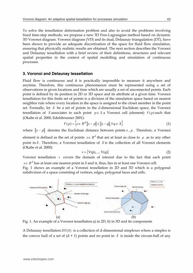
other simplex in )(SDT (okabe et. al 2000, Edelsbrunner 2001). A simplex is the convex hull of a set of (d + 1) points. For example, a 0D simplex is a point, a 1D simplex is a line segment, a 2D simplex is a triangle, and a 3D simplex is a tetrahedron (fig. 2).
(a) (b) (c) (d) Fig. 2. Simplex in a) 0D, b) 1D, c) 2D and d) 3D
)(SDT is unique, if S is a set of points in general position. This means no (d + 1) points are on the same hyperplane and no (d + 2) points are on the same ball. Therefore, a 2D Delaunay tessellation or Delaunay triangulation is a non-overlapping triangular subdivision of the space where each triangle has an empty circumcircle. The triangulation is unique, if no three (or more) points are collinear and no four (or more) points are on the same circumcircle. Similarity, a 3D Delaunay tessellation or Delaunay tetrahedralization is a non-overlapping tetrahedral subdivision of the space where each tetrahedron has an empty circumsphere. The tetrahedralization is unique, if no four (or more) points are coplanar and no five (or more) points are on the same circumsphere. Fig. 3 illustrates a 2D Delaunay triangulation and its components such as vertices, edges, triangles (elements).
(a) (b) Fig. 3. Delaunay tessellation a) in 2D and b) in 3D space and its components
3.1 Properties of Voronoi and Delaunay tessellations Voronoi and Delaunay tessellations have several interesting properties that make them attractive for numerical simulation methods: Duality between DT and VD: There is a connection between the Delaunay and the Voronoi tessellations called duality. The duality means that VD and DT are closely related graphs. The duality between VD and DT is based on some specific correspondences between geometric elements of the two data structures. This allows extracting the Voronoi tessellation from the Delaunay tessellation and vice versa. For a set of S points in a d-dimensional space, Delaunay tessellation can be obtained by joining all of pairs of points in
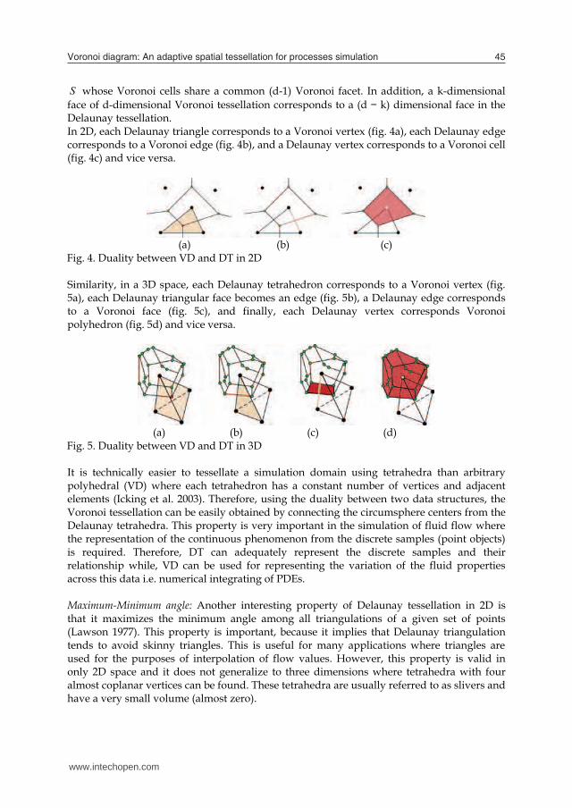
S whose Voronoi cells share a common (d-1) Voronoi facet. In addition, a k-dimensional face of d-dimensional Voronoi tessellation corresponds to a (d − k) dimensional face in the Delaunay tessellation. In 2D, each Delaunay triangle corresponds to a Voronoi vertex (fig. 4a), each Delaunay edge corresponds to a Voronoi edge (fig. 4b), and a Delaunay vertex corresponds to a Voronoi cell (fig. 4c) and vice versa.
(a) (b) (c)
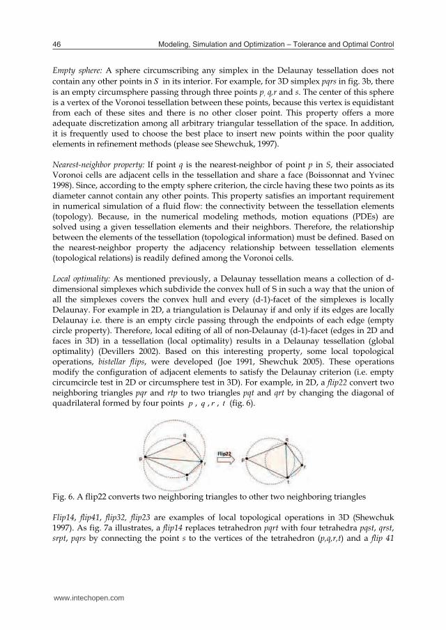
Fig. 4. Duality between VD and DT in 2D Similarity, in a 3D space, each Delaunay tetrahedron corresponds to a Voronoi vertex (fig. 5a), each Delaunay triangular face becomes an edge (fig. 5b), a Delaunay edge corresponds to a Voronoi face (fig. 5c), and finally, each Delaunay vertex corresponds Voronoi polyhedron (fig. 5d) and vice versa.
(a) (b) (c) (d) Fig. 5. Duality between VD and DT in 3D It is technically easier to tessellate a simulation domain using tetrahedra than arbitrary polyhedral (VD) where each tetrahedron has a constant number of vertices and adjacent elements (Icking et al. 2003). Therefore, using the duality between two data structures, the Voronoi tessellation can be easily obtained by connecting the circumsphere centers from the Delaunay tetrahedra. This property is very important in the simulation of fluid flow where the representation of the continuous phenomenon from the discrete samples (point objects) is required. Therefore, DT can adequately represent the discrete samples and their relationship while, VD can be used for representing the variation of the fluid properties across this data i.e. numerical integrating of PDEs. Maximum-Minimum angle: Another interesting property of Delaunay tessellation in 2D is that it maximizes the minimum angle among all triangulations of a given set of points (Lawson 1977). This property is important, because it implies that Delaunay triangulation tends to avoid skinny triangles. This is useful for many applications where triangles are used for the purposes of interpolation of flow values. However, this property is valid in only 2D space and it does not generalize to three dimensions where tetrahedra with four almost coplanar vertices can be found. These tetrahedra are usually referred to as slivers and have a very small volume (almost zero).
www.intechopen.com
Voronoi diagram: An adaptive spatial tessellation for processes simulation 45
other simplex in )(SDT (okabe et. al 2000, Edelsbrunner 2001). A simplex is the convex hull of a set of (d + 1) points. For example, a 0D simplex is a point, a 1D simplex is a line segment, a 2D simplex is a triangle, and a 3D simplex is a tetrahedron (fig. 2).
(a) (b) (c) (d) Fig. 2. Simplex in a) 0D, b) 1D, c) 2D and d) 3D
)(SDT is unique, if S is a set of points in general position. This means no (d + 1) points are on the same hyperplane and no (d + 2) points are on the same ball. Therefore, a 2D Delaunay tessellation or Delaunay triangulation is a non-overlapping triangular subdivision of the space where each triangle has an empty circumcircle. The triangulation is unique, if no three (or more) points are collinear and no four (or more) points are on the same circumcircle. Similarity, a 3D Delaunay tessellation or Delaunay tetrahedralization is a non-overlapping tetrahedral subdivision of the space where each tetrahedron has an empty circumsphere. The tetrahedralization is unique, if no four (or more) points are coplanar and no five (or more) points are on the same circumsphere. Fig. 3 illustrates a 2D Delaunay triangulation and its components such as vertices, edges, triangles (elements).
(a) (b) Fig. 3. Delaunay tessellation a) in 2D and b) in 3D space and its components
3.1 Properties of Voronoi and Delaunay tessellations Voronoi and Delaunay tessellations have several interesting properties that make them attractive for numerical simulation methods: Duality between DT and VD: There is a connection between the Delaunay and the Voronoi tessellations called duality. The duality means that VD and DT are closely related graphs. The duality between VD and DT is based on some specific correspondences between geometric elements of the two data structures. This allows extracting the Voronoi tessellation from the Delaunay tessellation and vice versa. For a set of S points in a d-dimensional space, Delaunay tessellation can be obtained by joining all of pairs of points in
S whose Voronoi cells share a common (d-1) Voronoi facet. In addition, a k-dimensional face of d-dimensional Voronoi tessellation corresponds to a (d − k) dimensional face in the Delaunay tessellation. In 2D, each Delaunay triangle corresponds to a Voronoi vertex (fig. 4a), each Delaunay edge corresponds to a Voronoi edge (fig. 4b), and a Delaunay vertex corresponds to a Voronoi cell (fig. 4c) and vice versa.
(a) (b) (c)
Fig. 4. Duality between VD and DT in 2D Similarity, in a 3D space, each Delaunay tetrahedron corresponds to a Voronoi vertex (fig. 5a), each Delaunay triangular face becomes an edge (fig. 5b), a Delaunay edge corresponds to a Voronoi face (fig. 5c), and finally, each Delaunay vertex corresponds Voronoi polyhedron (fig. 5d) and vice versa.
(a) (b) (c) (d) Fig. 5. Duality between VD and DT in 3D It is technically easier to tessellate a simulation domain using tetrahedra than arbitrary polyhedral (VD) where each tetrahedron has a constant number of vertices and adjacent elements (Icking et al. 2003). Therefore, using the duality between two data structures, the Voronoi tessellation can be easily obtained by connecting the circumsphere centers from the Delaunay tetrahedra. This property is very important in the simulation of fluid flow where the representation of the continuous phenomenon from the discrete samples (point objects) is required. Therefore, DT can adequately represent the discrete samples and their relationship while, VD can be used for representing the variation of the fluid properties across this data i.e. numerical integrating of PDEs. Maximum-Minimum angle: Another interesting property of Delaunay tessellation in 2D is that it maximizes the minimum angle among all triangulations of a given set of points (Lawson 1977). This property is important, because it implies that Delaunay triangulation tends to avoid skinny triangles. This is useful for many applications where triangles are used for the purposes of interpolation of flow values. However, this property is valid in only 2D space and it does not generalize to three dimensions where tetrahedra with four almost coplanar vertices can be found. These tetrahedra are usually referred to as slivers and have a very small volume (almost zero).
www.intechopen.com
Modeling, Simulation and Optimization – Tolerance and Optimal Control46
Empty sphere: A sphere circumscribing any simplex in the Delaunay tessellation does not contain any other points in S in its interior. For example, for 3D simplex pqrs in fig. 3b, there is an empty circumsphere passing through three points p, q,r and s. The center of this sphere is a vertex of the Voronoi tessellation between these points, because this vertex is equidistant from each of these sites and there is no other closer point. This property offers a more adequate discretization among all arbitrary triangular tessellation of the space. In addition, it is frequently used to choose the best place to insert new points within the poor quality elements in refinement methods (please see Shewchuk, 1997). Nearest-neighbor property: If point q is the nearest-neighbor of point p in S, their associated Voronoi cells are adjacent cells in the tessellation and share a face (Boissonnat and Yvinec 1998). Since, according to the empty sphere criterion, the circle having these two points as its diameter cannot contain any other points. This property satisfies an important requirement in numerical simulation of a fluid flow: the connectivity between the tessellation elements (topology). Because, in the numerical modeling methods, motion equations (PDEs) are solved using a given tessellation elements and their neighbors. Therefore, the relationship between the elements of the tessellation (topological information) must be defined. Based on the nearest-neighbor property the adjacency relationship between tessellation elements (topological relations) is readily defined among the Voronoi cells. Local optimality: As mentioned previously, a Delaunay tessellation means a collection of d-dimensional simplexes which subdivide the convex hull of S in such a way that the union of all the simplexes covers the convex hull and every (d-1)-facet of the simplexes is locally Delaunay. For example in 2D, a triangulation is Delaunay if and only if its edges are locally Delaunay i.e. there is an empty circle passing through the endpoints of each edge (empty circle property). Therefore, local editing of all of non-Delaunay (d-1)-facet (edges in 2D and faces in 3D) in a tessellation (local optimality) results in a Delaunay tessellation (global optimality) (Devillers 2002). Based on this interesting property, some local topological operations, bistellar flips, were developed (Joe 1991, Shewchuk 2005). These operations modify the configuration of adjacent elements to satisfy the Delaunay criterion (i.e. empty circumcircle test in 2D or circumsphere test in 3D). For example, in 2D, a flip22 convert two neighboring triangles pqr and rtp to two triangles pqt and qrt by changing the diagonal of quadrilateral formed by four points p , q , r , t (fig. 6).
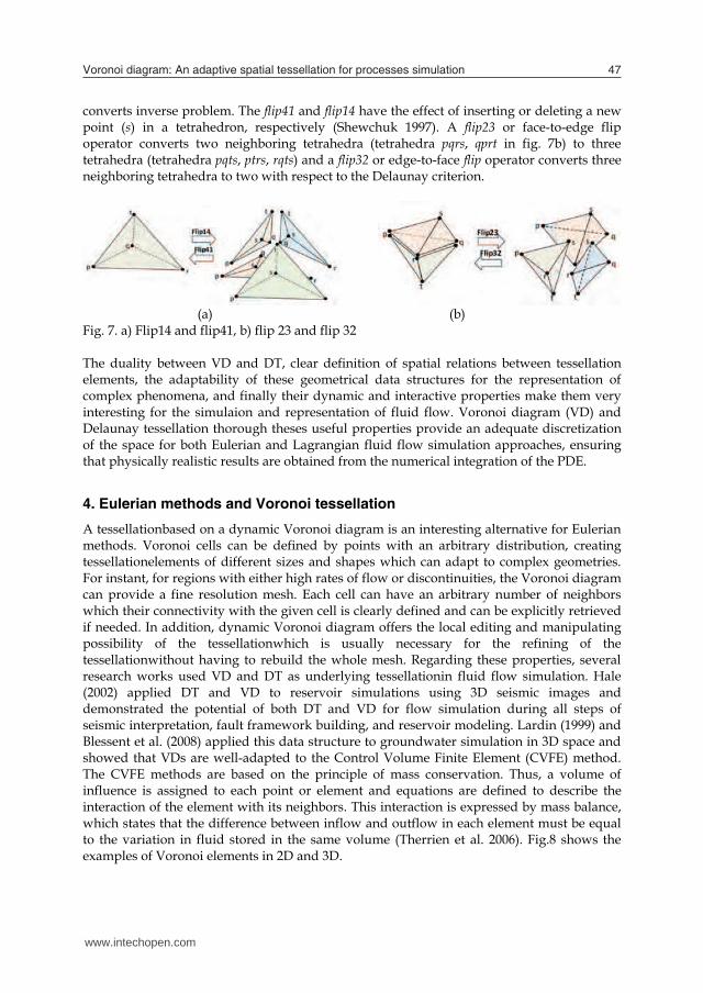
Fig. 6. A flip22 converts two neighboring triangles to other two neighboring triangles Flip14, flip41, flip32, flip23 are examples of local topological operations in 3D (Shewchuk 1997). As fig. 7a illustrates, a flip14 replaces tetrahedron pqrt with four tetrahedra pqst, qrst, srpt, pqrs by connecting the point s to the vertices of the tetrahedron (p,q,r,t) and a flip 41
converts inverse problem. The flip41 and flip14 have the effect of inserting or deleting a new point (s) in a tetrahedron, respectively (Shewchuk 1997). A flip23 or face-to-edge flip operator converts two neighboring tetrahedra (tetrahedra pqrs, qprt in fig. 7b) to three tetrahedra (tetrahedra pqts, ptrs, rqts) and a flip32 or edge-to-face flip operator converts three neighboring tetrahedra to two with respect to the Delaunay criterion.
(a) (b) Fig. 7. a) Flip14 and flip41, b) flip 23 and flip 32 The duality between VD and DT, clear definition of spatial relations between tessellation elements, the adaptability of these geometrical data structures for the representation of complex phenomena, and finally their dynamic and interactive properties make them very interesting for the simulaion and representation of fluid flow. Voronoi diagram (VD) and Delaunay tessellation thorough theses useful properties provide an adequate discretization of the space for both Eulerian and Lagrangian fluid flow simulation approaches, ensuring that physically realistic results are obtained from the numerical integration of the PDE.
4. Eulerian methods and Voronoi tessellation
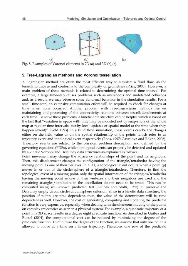
A tessellationbased on a dynamic Voronoi diagram is an interesting alternative for Eulerian methods. Voronoi cells can be defined by points with an arbitrary distribution, creating tessellationelements of different sizes and shapes which can adapt to complex geometries. For instant, for regions with either high rates of flow or discontinuities, the Voronoi diagram can provide a fine resolution mesh. Each cell can have an arbitrary number of neighbors which their connectivity with the given cell is clearly defined and can be explicitly retrieved if needed. In addition, dynamic Voronoi diagram offers the local editing and manipulating possibility of the tessellationwhich is usually necessary for the refining of the tessellationwithout having to rebuild the whole mesh. Regarding these properties, several research works used VD and DT as underlying tessellationin fluid flow simulation. Hale (2002) applied DT and VD to reservoir simulations using 3D seismic images and demonstrated the potential of both DT and VD for flow simulation during all steps of seismic interpretation, fault framework building, and reservoir modeling. Lardin (1999) and Blessent et al. (2008) applied this data structure to groundwater simulation in 3D space and showed that VDs are well-adapted to the Control Volume Finite Element (CVFE) method. The CVFE methods are based on the principle of mass conservation. Thus, a volume of influence is assigned to each point or element and equations are defined to describe the interaction of the element with its neighbors. This interaction is expressed by mass balance, which states that the difference between inflow and outflow in each element must be equal to the variation in fluid stored in the same volume (Therrien et al. 2006). Fig.8 shows the examples of Voronoi elements in 2D and 3D.
www.intechopen.com
Voronoi diagram: An adaptive spatial tessellation for processes simulation 47
Empty sphere: A sphere circumscribing any simplex in the Delaunay tessellation does not contain any other points in S in its interior. For example, for 3D simplex pqrs in fig. 3b, there is an empty circumsphere passing through three points p, q,r and s. The center of this sphere is a vertex of the Voronoi tessellation between these points, because this vertex is equidistant from each of these sites and there is no other closer point. This property offers a more adequate discretization among all arbitrary triangular tessellation of the space. In addition, it is frequently used to choose the best place to insert new points within the poor quality elements in refinement methods (please see Shewchuk, 1997). Nearest-neighbor property: If point q is the nearest-neighbor of point p in S, their associated Voronoi cells are adjacent cells in the tessellation and share a face (Boissonnat and Yvinec 1998). Since, according to the empty sphere criterion, the circle having these two points as its diameter cannot contain any other points. This property satisfies an important requirement in numerical simulation of a fluid flow: the connectivity between the tessellation elements (topology). Because, in the numerical modeling methods, motion equations (PDEs) are solved using a given tessellation elements and their neighbors. Therefore, the relationship between the elements of the tessellation (topological information) must be defined. Based on the nearest-neighbor property the adjacency relationship between tessellation elements (topological relations) is readily defined among the Voronoi cells. Local optimality: As mentioned previously, a Delaunay tessellation means a collection of d-dimensional simplexes which subdivide the convex hull of S in such a way that the union of all the simplexes covers the convex hull and every (d-1)-facet of the simplexes is locally Delaunay. For example in 2D, a triangulation is Delaunay if and only if its edges are locally Delaunay i.e. there is an empty circle passing through the endpoints of each edge (empty circle property). Therefore, local editing of all of non-Delaunay (d-1)-facet (edges in 2D and faces in 3D) in a tessellation (local optimality) results in a Delaunay tessellation (global optimality) (Devillers 2002). Based on this interesting property, some local topological operations, bistellar flips, were developed (Joe 1991, Shewchuk 2005). These operations modify the configuration of adjacent elements to satisfy the Delaunay criterion (i.e. empty circumcircle test in 2D or circumsphere test in 3D). For example, in 2D, a flip22 convert two neighboring triangles pqr and rtp to two triangles pqt and qrt by changing the diagonal of quadrilateral formed by four points p , q , r , t (fig. 6).
Fig. 6. A flip22 converts two neighboring triangles to other two neighboring triangles Flip14, flip41, flip32, flip23 are examples of local topological operations in 3D (Shewchuk 1997). As fig. 7a illustrates, a flip14 replaces tetrahedron pqrt with four tetrahedra pqst, qrst, srpt, pqrs by connecting the point s to the vertices of the tetrahedron (p,q,r,t) and a flip 41
converts inverse problem. The flip41 and flip14 have the effect of inserting or deleting a new point (s) in a tetrahedron, respectively (Shewchuk 1997). A flip23 or face-to-edge flip operator converts two neighboring tetrahedra (tetrahedra pqrs, qprt in fig. 7b) to three tetrahedra (tetrahedra pqts, ptrs, rqts) and a flip32 or edge-to-face flip operator converts three neighboring tetrahedra to two with respect to the Delaunay criterion.
(a) (b) Fig. 7. a) Flip14 and flip41, b) flip 23 and flip 32 The duality between VD and DT, clear definition of spatial relations between tessellation elements, the adaptability of these geometrical data structures for the representation of complex phenomena, and finally their dynamic and interactive properties make them very interesting for the simulaion and representation of fluid flow. Voronoi diagram (VD) and Delaunay tessellation thorough theses useful properties provide an adequate discretization of the space for both Eulerian and Lagrangian fluid flow simulation approaches, ensuring that physically realistic results are obtained from the numerical integration of the PDE.
4. Eulerian methods and Voronoi tessellation
A tessellationbased on a dynamic Voronoi diagram is an interesting alternative for Eulerian methods. Voronoi cells can be defined by points with an arbitrary distribution, creating tessellationelements of different sizes and shapes which can adapt to complex geometries. For instant, for regions with either high rates of flow or discontinuities, the Voronoi diagram can provide a fine resolution mesh. Each cell can have an arbitrary number of neighbors which their connectivity with the given cell is clearly defined and can be explicitly retrieved if needed. In addition, dynamic Voronoi diagram offers the local editing and manipulating possibility of the tessellationwhich is usually necessary for the refining of the tessellationwithout having to rebuild the whole mesh. Regarding these properties, several research works used VD and DT as underlying tessellationin fluid flow simulation. Hale (2002) applied DT and VD to reservoir simulations using 3D seismic images and demonstrated the potential of both DT and VD for flow simulation during all steps of seismic interpretation, fault framework building, and reservoir modeling. Lardin (1999) and Blessent et al. (2008) applied this data structure to groundwater simulation in 3D space and showed that VDs are well-adapted to the Control Volume Finite Element (CVFE) method. The CVFE methods are based on the principle of mass conservation. Thus, a volume of influence is assigned to each point or element and equations are defined to describe the interaction of the element with its neighbors. This interaction is expressed by mass balance, which states that the difference between inflow and outflow in each element must be equal to the variation in fluid stored in the same volume (Therrien et al. 2006). Fig.8 shows the examples of Voronoi elements in 2D and 3D.
www.intechopen.com
Modeling, Simulation and Optimization – Tolerance and Optimal Control48
(a) (b) (c) Fig. 8. Examples of Voronoi elements in 2D (a) and 3D (b),(c).
5. Free-Lagrangian methods and Voronoi tessellation
A Lagrangian method are often the most efficient way to simulate a fluid flow, as the tessellationmoves and conforms to the complexity of geometries (Price, 2005). However, a main problem of these methods is related to determining the optimal time interval. For example, a large time-step causes problems such as overshoots and undetected collisions and, as a result, we may observe some abnormal behavior in the simulation results. For a small time-step, an extensive computation effort will be required to check for changes at time when none occurred. Another problem with Free-Lagrangian methods lies on maintaining and processing of the connectivity relations between tessellationelements at each time. To solve these problems, a kinetic data structure can be helpful which is based on the fact that “variation in space with time may be modeled not by snap-shots of the whole map at regular time intervals, but by local updates of spatial model at the time when they happen (event)” (Gold 1993). In a fluid flow simulation, these events can be the changes either on the field value or on the spatial relationship of the points which refer to as trajectory event and topological event respectively (Roos, 1997; Gavrilova and Rokne, 2003). Trajectory events are related to the physical problem description and defined by the governing equations (PDEs), while topological events can properly be detected and updated by a kinetic Voronoi and Delaunay data structures as explained in follows. Point movement may change the adjacency relationships of the point and its neighbors. Then, this displacement changes the configuration of the triangle/tetrahedra having the moving point as one of their vertexes. In a DT, a topological event occurs when a point (p) moves in or out of the circle/sphere of a triangle/tetrahedron. Therefore, to find the topological event of a moving point, only the spatial information of the triangles/tetrahedra having the moving point as one of their vertexes and their neighbors are used and the remaining triangles/tetrahedra in the tessellation do not need to be tested. This can be computed using well-known predicted test (Guibas and Stolfi, 1985) to preserve the Delaunay empty circumcircle/circumsphere criterion. Since in a kinetic data structure, the position of points are time dependent, then, the value of the determinant will be time dependent as well. However, the cost of generating, computing and updating the predicate function is very expensive, especially when dealing with simultaneous moving of the points on complex trajectories as seen in a physical system. For example, a quadratic trajectory of a point in a 3D space results in a degree eight predicate function. As described in Guibas and Russel (2004), the computational cost can be reduced by minimizing the degree of the predicate function. To minimize the degree of the function, we assume that only one point is allowed to move at a time on a linear trajectory. Therefore, one row of the predicate
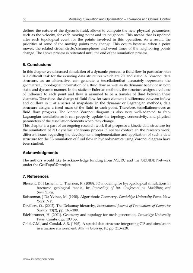
determinant must be allowed to vary linearly. Equation 1 shows the predicted function for a moving point in 3D Delaunay triangulation. According to this equation, a topological event for point p occurs when p moves in or moves out of the circumsphere of the tetrahedron, i.e. the value of the predicate function is 0.
0
1
1
1
1
1)()()()()()(
222
222
222
222
222
zyxzyx
zyxzyx
zyxzyx
zyxzyx
zyxzyx
dddddd
cccccc
bbbbbb
aaaaaa
tptptptptptp
(4)
Mostafavi and Gold (2003) have implemented a similar algorithm on the plan that minimizes the number of triangles which must be tested to detect the closest topological event of a moving point using a simple geometrical test. To do so, the algorithm computes the intersection between the trajectory of moving point p (a line segment) and some of the neighboring circumcircles cut the trajectory between the origin and the destination of the moving point. In fact, the triangles that the orthogonal projection of their circumcenter on the trajectory of p are behind the point p , with respect to the moving direction, are not considered. Then, every topological event which is the distance required for the moving point to cut the first circle on its trajectory is computed. Ledoux (2006) extended this algorithm to 3D for managing one moving point in 3D tessellation. However, there is a large number of moving points and topological events in a deforming kinetic spatial tessellation which must be managed in order to preserve the validity of the 3D tessellation. The sequence of the management of these events has an important impact on the simulation results. The topological events of all the moving points in the tessellation can be managed simultaneously using a priority queue data structure, where the moving points are organized with respect to their priority. This priority is defined based on the value of the simulation time (tsimulation) for each moving point. The simulation time is the total time that takes for each point to reach from its origin to its new location on the trajectory. Therefore, first, all the topological events of the moving points are computed. Next, the time taken for each point to reach its closest topological event eventt is obtained. This time depends on the velocity ( v ) of the moving point and the distance ( d ) between its current position and the location of its next closest topological event on its trajectory. We define the local time ( localt ) as the time that it takes for each point to move from its origin to its current position. The relation between these times is:
eventlocalsimulation ttt (5)
To facilitate the management of the topological events, we used a priority queues data structure by organizing the moving points based on the increasing value of simulationt . Therefore, the first member of the queue which has the smallest simulation time is processed first i.e. the moving point is moved to its new location and a local update is carried out for in the tessellation for the moving point and its neighbors. Following the topological changes in the tessellation, we need to update the physical parameters of the affected points. In a fluid flow simulation, the governing equation that
www.intechopen.com
Voronoi diagram: An adaptive spatial tessellation for processes simulation 49
(a) (b) (c) Fig. 8. Examples of Voronoi elements in 2D (a) and 3D (b),(c).
5. Free-Lagrangian methods and Voronoi tessellation
A Lagrangian method are often the most efficient way to simulate a fluid flow, as the tessellationmoves and conforms to the complexity of geometries (Price, 2005). However, a main problem of these methods is related to determining the optimal time interval. For example, a large time-step causes problems such as overshoots and undetected collisions and, as a result, we may observe some abnormal behavior in the simulation results. For a small time-step, an extensive computation effort will be required to check for changes at time when none occurred. Another problem with Free-Lagrangian methods lies on maintaining and processing of the connectivity relations between tessellationelements at each time. To solve these problems, a kinetic data structure can be helpful which is based on the fact that “variation in space with time may be modeled not by snap-shots of the whole map at regular time intervals, but by local updates of spatial model at the time when they happen (event)” (Gold 1993). In a fluid flow simulation, these events can be the changes either on the field value or on the spatial relationship of the points which refer to as trajectory event and topological event respectively (Roos, 1997; Gavrilova and Rokne, 2003). Trajectory events are related to the physical problem description and defined by the governing equations (PDEs), while topological events can properly be detected and updated by a kinetic Voronoi and Delaunay data structures as explained in follows. Point movement may change the adjacency relationships of the point and its neighbors. Then, this displacement changes the configuration of the triangle/tetrahedra having the moving point as one of their vertexes. In a DT, a topological event occurs when a point (p) moves in or out of the circle/sphere of a triangle/tetrahedron. Therefore, to find the topological event of a moving point, only the spatial information of the triangles/tetrahedra having the moving point as one of their vertexes and their neighbors are used and the remaining triangles/tetrahedra in the tessellation do not need to be tested. This can be computed using well-known predicted test (Guibas and Stolfi, 1985) to preserve the Delaunay empty circumcircle/circumsphere criterion. Since in a kinetic data structure, the position of points are time dependent, then, the value of the determinant will be time dependent as well. However, the cost of generating, computing and updating the predicate function is very expensive, especially when dealing with simultaneous moving of the points on complex trajectories as seen in a physical system. For example, a quadratic trajectory of a point in a 3D space results in a degree eight predicate function. As described in Guibas and Russel (2004), the computational cost can be reduced by minimizing the degree of the predicate function. To minimize the degree of the function, we assume that only one point is allowed to move at a time on a linear trajectory. Therefore, one row of the predicate
determinant must be allowed to vary linearly. Equation 1 shows the predicted function for a moving point in 3D Delaunay triangulation. According to this equation, a topological event for point p occurs when p moves in or moves out of the circumsphere of the tetrahedron, i.e. the value of the predicate function is 0.
0
1
1
1
1
1)()()()()()(
222
222
222
222
222
zyxzyx
zyxzyx
zyxzyx
zyxzyx
zyxzyx
dddddd
cccccc
bbbbbb
aaaaaa
tptptptptptp
(4)
Mostafavi and Gold (2003) have implemented a similar algorithm on the plan that minimizes the number of triangles which must be tested to detect the closest topological event of a moving point using a simple geometrical test. To do so, the algorithm computes the intersection between the trajectory of moving point p (a line segment) and some of the neighboring circumcircles cut the trajectory between the origin and the destination of the moving point. In fact, the triangles that the orthogonal projection of their circumcenter on the trajectory of p are behind the point p , with respect to the moving direction, are not considered. Then, every topological event which is the distance required for the moving point to cut the first circle on its trajectory is computed. Ledoux (2006) extended this algorithm to 3D for managing one moving point in 3D tessellation. However, there is a large number of moving points and topological events in a deforming kinetic spatial tessellation which must be managed in order to preserve the validity of the 3D tessellation. The sequence of the management of these events has an important impact on the simulation results. The topological events of all the moving points in the tessellation can be managed simultaneously using a priority queue data structure, where the moving points are organized with respect to their priority. This priority is defined based on the value of the simulation time (tsimulation) for each moving point. The simulation time is the total time that takes for each point to reach from its origin to its new location on the trajectory. Therefore, first, all the topological events of the moving points are computed. Next, the time taken for each point to reach its closest topological event eventt is obtained. This time depends on the velocity ( v ) of the moving point and the distance ( d ) between its current position and the location of its next closest topological event on its trajectory. We define the local time ( localt ) as the time that it takes for each point to move from its origin to its current position. The relation between these times is:
eventlocalsimulation ttt (5)
To facilitate the management of the topological events, we used a priority queues data structure by organizing the moving points based on the increasing value of simulationt . Therefore, the first member of the queue which has the smallest simulation time is processed first i.e. the moving point is moved to its new location and a local update is carried out for in the tessellation for the moving point and its neighbors. Following the topological changes in the tessellation, we need to update the physical parameters of the affected points. In a fluid flow simulation, the governing equation that
www.intechopen.com
Modeling, Simulation and Optimization – Tolerance and Optimal Control50
defines the nature of the dynamic fluid, allows to compute the new physical parameters, such as the velocity, for each moving point and its neighbors. This means that is updated after each topological event for the points involved in this operation. As a result, the priorities of some of the moving points may change. This occurs because, when a point moves, the related circumcircle/circumspheres and event times of the neighboring points change. The above process is reiterated until the end of the simulation process.
6. Conclusions
In this chapter we discussed simulation of a dynamic process , a fluid flow in particular, that is a difficult task for the exsisting data structures which are 2D and static. A Voronoi data structure, as an alternative, can generate a tessellationthat accurately represents the geometrical, topological information of a fluid flow as well as its dynamic behavior in both static and dynamic manner. In the static or Eulerian methods, the structure assigns a volume of influence to each point and flow is assumed to be a transfer of fluid between these elements. Therefore, the change of fluid flow for each element is difference between inflow and outflow in it at a series of snapshots. In the dynamic or Lagrangian methods, data structure assigns a fixed mass of the fluid to each point. Therefore, tessellationmoves as fluid flow progress. The kinetic Voronoi diagram is also very well-adapted to free-Lagrangian tessellationas it can properly update the topology, connectivity, and physical parameters of the tessellationelements when they change. This chapter is a part of an ongoing research work that proposes a kinetic data structure for the simulation of 3D dynamic contionus process in spatial context. In the research work, different issues regarding the development, implementation and application of such a data structure for the 3D simulation of fluid flow in hydrodynamics using Voronoi diagram have been studied. Acknowledgments
The authors would like to acknowledge funding from NSERC and the GEOIDE Network under the GeoTopo3D project.
7. References
Blessent, D.; Hashemi, L.; Therrien, R. (2008). 3D modeling for hyrogeological simulations in fractured geological media, In: Proceeding of Int. Conference on Modelling and Simulation.
Boissonnat, J.D.; Yvinec, M. (1998). Algorithmic Geometry, Cambridge University Press, New York, NY.
Devillers, O., (2002). The Delaunay hierarchy, International Journal of Foundations of Computer Science, 13(2), pp. 163–180.
Edelsbrunner, H. (2001). Geometry and topology for mesh generation, Cambridge University Press, Cambridge, 190 pp.
Gold, C.M., and Condal, A.R. (1995). A spatial data structure integrating GIS and simulation in a marine environment, Marine Geodesy, 18, pp. 213–228.
Gold, C.M. (1993). An outline of an event-driven spatial data structure for managing time varying maps, In: Proceeding: Canadian conference on GIS, pp.880-888.
Guibas, LJ., and Russel, D. (2004). An empirical comparison of techniques for updating Delaunay triangulations, Symposium on Computational Geometry, pp.170-179.
Guibas, L.J., Stolfi, J. (1985). Primitives for the manipulation of general subdivisions and the computation of Voronoi diagrams, ACM Transactions on Graphics, 4, 74–123.
Hale, D. (2002). Atomic meshes: from seismic imaging to reservoir simulation, In: Proceedings of the 8th European Conference on the Mathematics of Oil Recovery.
Hashemi, L., and Mostafavi, M.A. (2008). A kinetic spatial data structure in support of a 3D Free Lagrangian hydrodynamics algorithm, In: Proceeding of Int. Conference on Applied Modeling and Simulation.
Icking, C.; Klein, R.; Köllner, P.; Ma, L. (2003). Java applets for the dynamic visualization of Voronoi diagrams, in: Lecture Notes in Computer Science, pp. 191 – 205.
Joe, B. (1991). Construction of three-dimensional Delaunay triangulations using local transformations, Computer Aided Geometric Design, 8(2), pp. 123-142.
Knupp, P.(1996). A moving mesh algorithm for 3D regional groundwater flow with water table and seepage face, International Journal for Numerical Methods in Fluids 19(2), pp. 83-95.
Lawson, C.L.(1977), Software for C1 Surface Interpolation, in: Rive, J. (Ed.) Mathematical Software III, Academic Press, New York, pp. 161-194.
Ledoux, H. (2006). Modelling Three-dimensional Fields in Geosciences with the Voronoi Diagram and its Dual, Ph.D. thesis, University of Glamorgan.
Malcevic, O. G. (2002). Dynamic-mesh finite element method for Lagrangian computational fluid dynamics, Advances in Water Resources 38, pp. 965-982.
Mostafavi, M.A. (2002). Development of a global dynamic data structure, PhD thesis, university of Laval, Canada.
Mostafavi, M.A., and Gold, C. M. (2004). A Global Spatial Data Structure for Marine Simulation, Intl J Geographical Information Science, 18, pp. 211-227.
Neuman, S.P., (1984). Adaptive Eulerian-Lagrangian finite element method for advection-dispersion, International Journal for Numerical Methods in Engineering, 20, pp. 321-337.
Okabe, A.; Boots, B.; Sugihara, K. and Chiu, S.N. (2000). Spatial tessellations: concepts and applications of Voronoi Diagrams, John Wiley & Sons, Chichester, West Sussex, England.
Price, J.F., (2005). Lagrangian and Eulerian representations of fluid flow: Part I, kinematics and the equations of Motion.
Roos, T. (1997). New upper bounds on Voronoi diagrams of moving points, Nordic J Computing, 4, pp. 167-171.
Shewchuk, R. (1997). Delaunay refinement mesh generation, PhD Thesis, Carnegie Mellon University.
Shewchuk, R. (2005). Star splaying: an algorithm for repairing Delaunay triangulation and convexhulls, In: Proceeding of the Twenty-First Annual ACM symposium on Computational Geometry, ACM Press New York, pp.237-246.
Therrien, R.; McLaren, R.G.; Sudicky, E.A.; Panday, S.M. (2006). HydroSphere: A three-dimensional numerical model describing fully-integrated subsurface and surface Flow and solute Transport, User’s manual.
www.intechopen.com
Voronoi diagram: An adaptive spatial tessellation for processes simulation 51
defines the nature of the dynamic fluid, allows to compute the new physical parameters, such as the velocity, for each moving point and its neighbors. This means that is updated after each topological event for the points involved in this operation. As a result, the priorities of some of the moving points may change. This occurs because, when a point moves, the related circumcircle/circumspheres and event times of the neighboring points change. The above process is reiterated until the end of the simulation process.
6. Conclusions
In this chapter we discussed simulation of a dynamic process , a fluid flow in particular, that is a difficult task for the exsisting data structures which are 2D and static. A Voronoi data structure, as an alternative, can generate a tessellationthat accurately represents the geometrical, topological information of a fluid flow as well as its dynamic behavior in both static and dynamic manner. In the static or Eulerian methods, the structure assigns a volume of influence to each point and flow is assumed to be a transfer of fluid between these elements. Therefore, the change of fluid flow for each element is difference between inflow and outflow in it at a series of snapshots. In the dynamic or Lagrangian methods, data structure assigns a fixed mass of the fluid to each point. Therefore, tessellationmoves as fluid flow progress. The kinetic Voronoi diagram is also very well-adapted to free-Lagrangian tessellationas it can properly update the topology, connectivity, and physical parameters of the tessellationelements when they change. This chapter is a part of an ongoing research work that proposes a kinetic data structure for the simulation of 3D dynamic contionus process in spatial context. In the research work, different issues regarding the development, implementation and application of such a data structure for the 3D simulation of fluid flow in hydrodynamics using Voronoi diagram have been studied. Acknowledgments
The authors would like to acknowledge funding from NSERC and the GEOIDE Network under the GeoTopo3D project.
7. References
Blessent, D.; Hashemi, L.; Therrien, R. (2008). 3D modeling for hyrogeological simulations in fractured geological media, In: Proceeding of Int. Conference on Modelling and Simulation.
Boissonnat, J.D.; Yvinec, M. (1998). Algorithmic Geometry, Cambridge University Press, New York, NY.
Devillers, O., (2002). The Delaunay hierarchy, International Journal of Foundations of Computer Science, 13(2), pp. 163–180.
Edelsbrunner, H. (2001). Geometry and topology for mesh generation, Cambridge University Press, Cambridge, 190 pp.
Gold, C.M., and Condal, A.R. (1995). A spatial data structure integrating GIS and simulation in a marine environment, Marine Geodesy, 18, pp. 213–228.
Gold, C.M. (1993). An outline of an event-driven spatial data structure for managing time varying maps, In: Proceeding: Canadian conference on GIS, pp.880-888.
Guibas, LJ., and Russel, D. (2004). An empirical comparison of techniques for updating Delaunay triangulations, Symposium on Computational Geometry, pp.170-179.
Guibas, L.J., Stolfi, J. (1985). Primitives for the manipulation of general subdivisions and the computation of Voronoi diagrams, ACM Transactions on Graphics, 4, 74–123.
Hale, D. (2002). Atomic meshes: from seismic imaging to reservoir simulation, In: Proceedings of the 8th European Conference on the Mathematics of Oil Recovery.
Hashemi, L., and Mostafavi, M.A. (2008). A kinetic spatial data structure in support of a 3D Free Lagrangian hydrodynamics algorithm, In: Proceeding of Int. Conference on Applied Modeling and Simulation.
Icking, C.; Klein, R.; Köllner, P.; Ma, L. (2003). Java applets for the dynamic visualization of Voronoi diagrams, in: Lecture Notes in Computer Science, pp. 191 – 205.
Joe, B. (1991). Construction of three-dimensional Delaunay triangulations using local transformations, Computer Aided Geometric Design, 8(2), pp. 123-142.
Knupp, P.(1996). A moving mesh algorithm for 3D regional groundwater flow with water table and seepage face, International Journal for Numerical Methods in Fluids 19(2), pp. 83-95.
Lawson, C.L.(1977), Software for C1 Surface Interpolation, in: Rive, J. (Ed.) Mathematical Software III, Academic Press, New York, pp. 161-194.
Ledoux, H. (2006). Modelling Three-dimensional Fields in Geosciences with the Voronoi Diagram and its Dual, Ph.D. thesis, University of Glamorgan.
Malcevic, O. G. (2002). Dynamic-mesh finite element method for Lagrangian computational fluid dynamics, Advances in Water Resources 38, pp. 965-982.
Mostafavi, M.A. (2002). Development of a global dynamic data structure, PhD thesis, university of Laval, Canada.
Mostafavi, M.A., and Gold, C. M. (2004). A Global Spatial Data Structure for Marine Simulation, Intl J Geographical Information Science, 18, pp. 211-227.
Neuman, S.P., (1984). Adaptive Eulerian-Lagrangian finite element method for advection-dispersion, International Journal for Numerical Methods in Engineering, 20, pp. 321-337.
Okabe, A.; Boots, B.; Sugihara, K. and Chiu, S.N. (2000). Spatial tessellations: concepts and applications of Voronoi Diagrams, John Wiley & Sons, Chichester, West Sussex, England.
Price, J.F., (2005). Lagrangian and Eulerian representations of fluid flow: Part I, kinematics and the equations of Motion.
Roos, T. (1997). New upper bounds on Voronoi diagrams of moving points, Nordic J Computing, 4, pp. 167-171.
Shewchuk, R. (1997). Delaunay refinement mesh generation, PhD Thesis, Carnegie Mellon University.
Shewchuk, R. (2005). Star splaying: an algorithm for repairing Delaunay triangulation and convexhulls, In: Proceeding of the Twenty-First Annual ACM symposium on Computational Geometry, ACM Press New York, pp.237-246.
Therrien, R.; McLaren, R.G.; Sudicky, E.A.; Panday, S.M. (2006). HydroSphere: A three-dimensional numerical model describing fully-integrated subsurface and surface Flow and solute Transport, User’s manual.
www.intechopen.com

Modeling, Simulation and Optimization – Tolerance and Optimal Control52
Whitehurst, R. (1995). A Free-lagrangian method for gas dynamics, Mon. Not. R. Astron. Soc. 277, pp. 655-680.
Zegeling, A.; Verwer, J.G. and Eijkeren, J.C.H. (1992). Application of a moving grid method to a class of 1D brine transport problems in porous media, International Journal for Numerical Methods in Fluids, 15, pp. 175-191.
www.intechopen.com
Modeling Simulation and Optimization - Tolerance and OptimalControlEdited by Shkelzen Cakaj
ISBN 978-953-307-056-8Hard cover, 304 pagesPublisher InTechPublished online 01, April, 2010Published in print edition April, 2010
InTech EuropeUniversity Campus STeP Ri Slavka Krautzeka 83/A 51000 Rijeka, Croatia Phone: +385 (51) 770 447 Fax: +385 (51) 686 166www.intechopen.com
InTech ChinaUnit 405, Office Block, Hotel Equatorial Shanghai No.65, Yan An Road (West), Shanghai, 200040, China
Phone: +86-21-62489820 Fax: +86-21-62489821
Parametric representation of shapes, mechanical components modeling with 3D visualization techniques usingobject oriented programming, the well known golden ratio application on vertical and horizontal displacementinvestigations of the ground surface, spatial modeling and simulating of dynamic continuous fluid flow process,simulation model for waste-water treatment, an interaction of tilt and illumination conditions at flight simulationand errors in taxiing performance, plant layout optimal plot plan, atmospheric modeling for weather prediction,a stochastic search method that explores the solutions for hill climbing process, cellular automata simulations,thyristor switching characteristics simulation, and simulation framework toward bandwidth quantization andmeasurement, are all topics with appropriate results from different research backgrounds focused on toleranceanalysis and optimal control provided in this book.
How to referenceIn order to correctly reference this scholarly work, feel free to copy and paste the following:
Leila Hashemi Beni, Mir Abolfazl Mostafavi and Jacynthe Pouliot (2010). Voronoi diagram: An adaptive spatialtessellation for processes simulation, Modeling Simulation and Optimization - Tolerance and Optimal Control,Shkelzen Cakaj (Ed.), ISBN: 978-953-307-056-8, InTech, Available from:http://www.intechopen.com/books/modeling-simulation-and-optimization-tolerance-and-optimal-control/voronoi-diagram-an-adaptive-spatial-tessellation-for-processes-simulation

© 2010 The Author(s). Licensee IntechOpen. This chapter is distributedunder the terms of the Creative Commons Attribution-NonCommercial-ShareAlike-3.0 License, which permits use, distribution and reproduction fornon-commercial purposes, provided the original is properly cited andderivative works building on this content are distributed under the samelicense.


![Generalized Voronoi Tessellation as a Model of Two ...dynamics, evolving multicellular tissue was represented by Voronoi tessellations [18]. In particular, growth instabilities, blastula](https://static.fdocuments.in/doc/165x107/5fa935791fdd165b3a3ba749/generalized-voronoi-tessellation-as-a-model-of-two-dynamics-evolving-multicellular.jpg)