Volumetric Guidance for Handling Triple Products in ...

Volumetric Guidance for Handling Triple Productsin Spatial Branch-and-Bound

by

Emily E. Speakman

A dissertation submitted in partial fulfillmentof the requirements for the degree of

Doctor of Philosophy(Industrial and Operations Engineering)

in The University of Michigan2017

Doctoral Committee:

Professor Jon Lee, ChairAssociate Professor Kevin J. ComptonAssociate Professor Marina A. EpelmanAssistant Professor Siqian M. Shen

Emily E. Speakman

ORCID iD: 0000-0002-7352-1355

c© Emily E. Speakman 2017

All Rights Reserved

ACKNOWLEDGEMENTS

First, I would like to thank my advisor, Professor Jon Lee. His guidance and

direction have been invaluable throughout this journey, and I truly can’t imagine

having undertaken this process without his mentorship. Any amount of success I

may have, either now or in the future, also belongs to him.

Secondly, thank you to Mr. Harris, who made me want to pursue mathematics,

and to all my teachers, advisors, and professors after that, who prepared me for my

studies at Michigan. In particular, I owe much gratitude to Jill Hardin Wilson. She

believed I could do this well before it even occurred to me to believe in myself. I

wouldn’t be here without her.

Thank you to my committee members, Professor Marina Epelman, Professor

Siqian Shen, and Professor Kevin Compton, not only for participating in my de-

fense, but for your courses and input throughout my time here. Between the three of

you, I have learned an enormous amount. Thank you as well to all the faculty, staff,

and students in the IOE department, for being there throughout the past five years.

This experience would not have been all that it was without you.

I would certainly never have made it to this point without my friends and family.

I will avoid using names in the fear that I may miss someone out, but to those of

you far away: thank you. You have supported me, cheered for me and visited me

despite the distance. It is impossible for me to overstate my appreciation for you. To

my friends in Ann Arbor: you have kept me encouraged even during the low points.

Thank you for making this place a second home.

To mum and dad, with more love and gratitude than I can ever express, no one

could ask for more supportive parents than the two of you.

Finally, I give thanks to God, who holds all things together.

In addition, I gratefully acknowledge partial support from NSF grant CMMI1160915, ONR grant

N00014-14-1-0315, a Rackham Summer Award, and the Dwight F. Benton Fellowship.

ii

TABLE OF CONTENTS

ACKNOWLEDGEMENTS . . . . . . . . . . . . . . . . . . . . . . . . . . ii

LIST OF FIGURES . . . . . . . . . . . . . . . . . . . . . . . . . . . . . . . v

LIST OF TABLES . . . . . . . . . . . . . . . . . . . . . . . . . . . . . . . . vii

ABSTRACT . . . . . . . . . . . . . . . . . . . . . . . . . . . . . . . . . . . viii

CHAPTER

1. Introduction . . . . . . . . . . . . . . . . . . . . . . . . . . . . . . 1

1.1 Thesis overview . . . . . . . . . . . . . . . . . . . . . . . . . 7

2. Preliminaries . . . . . . . . . . . . . . . . . . . . . . . . . . . . . . 8

2.1 Double McCormick . . . . . . . . . . . . . . . . . . . . . . . . 82.1.1 Convexification . . . . . . . . . . . . . . . . . . . . 92.1.2 Hull . . . . . . . . . . . . . . . . . . . . . . . . . . . 10

2.2 Alternatives . . . . . . . . . . . . . . . . . . . . . . . . . . . . 12

3. Volume Formulae . . . . . . . . . . . . . . . . . . . . . . . . . . . 14

3.1 Introduction . . . . . . . . . . . . . . . . . . . . . . . . . . . 143.2 Theorems . . . . . . . . . . . . . . . . . . . . . . . . . . . . . 143.3 Proof of Thm. 3.1 . . . . . . . . . . . . . . . . . . . . . . . . 17

3.3.1 An interesting note about Ph . . . . . . . . . . . . . 243.4 Proof of Thm. 3.4 . . . . . . . . . . . . . . . . . . . . . . . . 25

3.4.1 Keeping track of facets . . . . . . . . . . . . . . . . 323.5 Proof of Thm. 3.2 . . . . . . . . . . . . . . . . . . . . . . . . 37

3.5.1 Keeping track of facets . . . . . . . . . . . . . . . . 463.6 Proof of Thm. 3.3 . . . . . . . . . . . . . . . . . . . . . . . . 543.7 Concluding remarks and future work . . . . . . . . . . . . . . 543.8 Technical lemmas . . . . . . . . . . . . . . . . . . . . . . . . 55

3.8.1 Useful lemmas . . . . . . . . . . . . . . . . . . . . . 56

iii

3.8.2 Proving non-negativity . . . . . . . . . . . . . . . . 56

4. Experimental Justification of Volume . . . . . . . . . . . . . . . 64

4.1 Introduction . . . . . . . . . . . . . . . . . . . . . . . . . . . 644.2 Measuring relaxations via volume in mathematical optimization 644.3 Box cubic programming problems . . . . . . . . . . . . . . . . 654.4 From volume to objective function gap . . . . . . . . . . . . . 664.5 Computational experiments . . . . . . . . . . . . . . . . . . . 67

4.5.1 Box cubic programming problems and four relaxations 674.5.2 Three scenarios for the hypergraph H . . . . . . . . 684.5.3 Quality of relaxations . . . . . . . . . . . . . . . . . 694.5.4 Validating the relationship between volume and ob-

jective gap . . . . . . . . . . . . . . . . . . . . . . . 704.5.5 A worst case . . . . . . . . . . . . . . . . . . . . . . 71

4.6 Concluding remarks and future work . . . . . . . . . . . . . . 81

5. Using Volume to Guide Branching-Point Selection . . . . . . 82

5.1 Introduction . . . . . . . . . . . . . . . . . . . . . . . . . . . 825.2 Current branching practice . . . . . . . . . . . . . . . . . . . 825.3 Results . . . . . . . . . . . . . . . . . . . . . . . . . . . . . . 84

5.3.1 The convex-hull convexification . . . . . . . . . . . 855.3.2 The best double-McCormick convexification . . . . . 99

5.4 Concluding remarks and future work . . . . . . . . . . . . . . 1025.5 Technical propositions, lemmas, and theorems . . . . . . . . . 103

5.5.1 Convex-hull convexification . . . . . . . . . . . . . . 1035.5.2 Double-McCormick convexification . . . . . . . . . . 107

BIBLIOGRAPHY . . . . . . . . . . . . . . . . . . . . . . . . . . . . . . . . 114

iv

LIST OF FIGURES

1.1 An example of a DAG for the function f =x31e

x2

sin(x2x3). . . . . . . . . 3

1.2 Convexifying and reconvexifying after branching in sBB . . . . . . . 4

3.1 Difference in volume between P3 and P1

(3a3(b3−a3)2

24b3

)vs. parameters

a3 and b3 (a1 = a2 = 0 and b1 = b2 = 1) . . . . . . . . . . . . . . . . 18

3.2 Visual representation of the convex-hull extreme points . . . . . . . 19

3.3 Visual representation of adding point v8 to simplex S . . . . . . . . 20

3.4 Visual representation of adding points v3 and v7 to polytope Q . . . 22

3.5 The line segment between v3 and v7 intersects polytope Q . . . . . 23

3.6 Visual representation of the convex-hull polytope . . . . . . . . . . 25

3.7 Visual representation of the convex-hull polytope (blue) and the four‘extra’ extreme points of P3 . . . . . . . . . . . . . . . . . . . . . . 26

3.8 For Table 3.1 . . . . . . . . . . . . . . . . . . . . . . . . . . . . . . 27

3.9 For Table 3.2 . . . . . . . . . . . . . . . . . . . . . . . . . . . . . . 38

4.1 Quasi-mean-width differences . . . . . . . . . . . . . . . . . . . . . 73

4.2 Quasi-mean-width performance profiles . . . . . . . . . . . . . . . . 74

4.3 Idealized radius predicting quasi mean width . . . . . . . . . . . . . 76

4.4 Idealized radial distance predicting quasi mean width difference . . 78

4.5 Worst-case analysis for a3 (a1 = a2 = 0, b1 = b2 = 1) . . . . . . . . . 80

v

5.1 Variable labeling as the branching point varies in Case 0 . . . . . . 86

5.2 Variable labeling as the branching point varies in Case 1 and Case 2 86

5.3 Illustration of a continuous piecewise-quadratic function . . . . . . . 88

5.4 Picture to illustrate the possible outcomes of Algorithm 1 in Case 1 93

5.5 Plot of the total volume function for parameter values: (a1 = 0, b1 =1, a2 = 0, b2 = 1, a3 = 0, b3 = 1) . . . . . . . . . . . . . . . . . . . . . 94

5.6 Illustration of a globally convex piecewise-quadratic function . . . . 95

5.7 Case analysis for P3 . . . . . . . . . . . . . . . . . . . . . . . . . . . 100

vi

LIST OF TABLES

3.1 Summary of midpoint substitutions for Thm. 3.4 . . . . . . . . . . 27

3.2 Summary of midpoint substitutions for Thm. 3.2 . . . . . . . . . . 38

5.1 Default parameter settings . . . . . . . . . . . . . . . . . . . . . . . 83

vii

ABSTRACT

Volumetric Guidance for Handling Triple Products in Spatial Branch-and-Bound

by

Emily E. Speakman

Chair: Jon Lee

Spatial branch-and-bound (sBB) is the workhorse algorithmic framework used to

globally solve mathematical mixed-integer non-linear optimization (MINLO) prob-

lems. Formulating a problem using this paradigm allows both the non-linearities

of a system and any discrete design choices to be modeled effectively. Because of

the generality of this approach, MINLO is used in a wide variety of applications,

from chemical engineering problems and network design, to medical applications and

problems in the airline industry.

Due in part to their generality (and therefore wide applicability), MINLO prob-

lems are very difficult in general, and consequently, the best ways to implement many

details of sBB are not wholly understood. In this work, we provide analytic results

guiding the implementation of sBB for a simple but frequently occurring function

building block. As opposed to computationally demonstrating that our techniques

work only for a particular set of test problems, we analytically establish results that

hold for all problems of the given form. In this way, we also demonstrate that analytic

results are indeed obtainable for certain sBB implementation decisions.

In particular, we use volume as a geometric measure to compare different con-

vex relaxations for functions involving trilinear monomials (or any three quantities

viii

multiplied together). We consider different choices for convexifying the graph of a

triple product (i.e. f = x1x2x3), and obtain formulae for the volume (in terms of the

variable upper and lower bounds) for each of these convexifications. We are then able

to order the convexifications with regard to their volume. We also provide computa-

tional evidence to support our choice of volume as an effective comparison measure,

and show that in the context of triple products, volume is an excellent predictor of

the objective function gap. Finally, we use the volume measure to provide guidance

regarding branching-point selection in the implementation of sBB.

ix

CHAPTER 1

Introduction

Mathematical optimization is a commonly used and powerful paradigm for model-

ing and solving a variety of important applied problems. The inherent non-linearities

and discrete decisions in many aspects of the real world mean that numerous im-

portant problems can be solved by globally optimizing a mixed-integer non-linear

optimization (MINLO) problem. Therefore, it is important that we understand how

to simultaneously deal with both the discrete and the non-linear aspects of these

problems to design efficient algorithms.

To quote R. T. Rockafellar ([43]) “...the great watershed in optimization isn’t

between linearity and non-linearity, but convexity and non-convexity.” This is what

makes MINLO problems especially hard — they can contain non-convexity in the

form of integer variables, and also in the structure of the objective and constraint

functions themselves. Seeking to handle broad classes of non-convex functions im-

plies that state-of-the-art software can only hope to routinely succeed on relatively

small problem instances, and that research has great potential to achieve significant

improvements on current performance. A well-studied example where these non-

convexities occur is the pooling problem, an important application arising from chem-

ical engineering (see [38] for a survey), but non-convex functions feature in many other

formulations including the network design of gas ([28]), energy ([21]), and transporta-

tion ([16]) networks. For a survey of important applications in non-convex MINLO,

see §2 of [9]. Many of these applications require us to find good solutions quickly,

and to react to new data as we obtain it. By harnessing both growing computational

power and theoretical insights to improve solution methods, we can hope for a great

impact on the tractability of a host of applied problems.

1

A MINLO problem has the form:

minx∈Zn, y∈Rm

f(x, y) : (x, y) ∈ F

,

where f : Zn × Rm → R and F ⊆ Zn × Rm. The only assumptions we make on the

function f and the functions that describe F are that they are factorable (see [32]).

A function is factorable with respect to a library of low-dimensional functions, e.g.,

sin(x), ln(x), arctan(x), xy, xyz, xy, ..., if it can be composed from these functions in

a finite number of steps by introducing an appropriate number of auxiliary variables.

For example:

f =x31e

x2

sin(x2x3)→ f = y1y2y5, y5 =

1

y4, y4 = sin(y3), y3 = x2x3, y2 = ex2 , y1 = x31.

The assumption that our functions are factorable is quite unrestrictive, and many

functions of interest meet this requirement. We note that the determinant of a matrix

is a factorable function, but the factorization is unreasonable. ‘Finite’ could clearly

be very large, so in practice we require that our functions can be computed in a ‘rea-

sonable’ number of steps; how we define reasonable can depend on the problem, but

could mean, for example, logarithmic in the number of model variables. Additionally,

we assume that we have convexification methods for the graphs of the functions in our

library (often linearizations), and that we can combine them to build convexifications

of the graphs of the functions in the optimization problem.

Spatial branch-and-bound (sBB) (see [1, 45, 53]) is the workhorse general-purpose

algorithm in the area of global optimization. It works by using additional variables

to reformulate every function of the formulation as a (labeled) directed acyclic graph

(DAG). Root nodes can be very complicated functions, and leaves are variables that

appear in the input formulation, each labeled with its interval domain. Intermedi-

ate nodes are labeled with auxiliary variables together with operators from a small

dictionary of basic functions of few (often one, two, or three) variables. See Fig-

ure 1.1 for an example of a DAG for the factorable function we considered above,

f =x31e

x2

sin(x2x3). As noted, we assume that we have a method for convexifying the graph

of each dictionary function. sBB algorithms work by composing convex relaxations

of the dictionary functions, according to the DAG, to get relaxations of the root

functions. Bounds on the leaves propagate to other nodes and conversely. Branch-

ing (subdividing the domain interval of a variable) creates subproblems, which are

treated recursively. Objective bounds for subproblems are appropriately combined to

2

f =x31e

x2

sin(x2x3)

(·)× (·)× (·)

x1

x1 ∈ [a1, b1]

y1 = x31

(·)3y2 = ex2

e(·)

y5 = 1sin(x2x3)

1(·)

x2

x2 ∈ [a2, b2]

y4 = sin (x2x3)

sin (·)

y3 = x2x3

(·)× (·)

x3

x3 ∈ [a3, b3]

Figure 1.1: An example of a DAG for the function f =x31e

x2

sin(x2x3)

achieve a global-optimization algorithm.

Figure 1.2 illustrates an example of a univariate function. Here, the sBB algorithm

obtains a lower bound for the non-convex blue function by convexifying its graph.

The red region is a convexification of the graph of the blue function over the whole

domain shown, and the minimum over this set is a lower bound on the value of the

blue function over the domain. However, by branching, reconvexifying, and obtaining

the two green convex regions, we obtain a tighter lower bound on the blue function

(the minimum of the respective minimums over the two green convex regions).

Much of the research on sBB has focused on developing tight convexifications

for basic functions of few variables (many references can be found in [11]). Other

research has focused on how bounds can be efficiently propagated and how branching

can be judiciously be carried out (see [6], for example). From the viewpoint of good

convexifications, much less attention has been paid to how the DAGs are created,

but this can have a strong impact on the quality of the resulting convex relaxation of

the input formulation; see [29, 30, 50, 62] for some key papers with other viewpoints

concerning constructing DAGs.

3

Figure 1.2: Convexifying and reconvexifying after branching in sBB

For basic multilinear monomials f(x1, . . . , xn) := x1 · · ·xn, with xi ∈ [ai, bi],

there is already a lot of flexibility which can have a significant impact on the over-

all convexification of the graph of f(x1, . . . , xn) := x1 · · ·xn on the box domain

[a1, b1] × · · · × [an, bn]. For n = 2, we have the classic McCormick inequalities, see

[32], which simply describe the tetrahedron that is the convex hull of the four points

(f, x1, x2) := (a1a2, a1, a2), (a1b2, a1, b2), (b1a2, b1, a2), (b1b2, b1, b2),

see [3]. The inequalities can be derived from the four inequalities

(x1 − a1)(x2 − a2) ≥ 0, (x1 − a1)(b2 − x2) ≥ 0,

(b1 − x1)(x2 − a2) ≥ 0, (b1 − x1)(b2 − x2) ≥ 0,

by multiplying out and then replacing all occurrences of x1x2 by the variable f . This

4

gives the following linear inequalities:

f − a2x1 − a1x2 + a1a2 ≥ 0,

−f + b2x1 + a1x2 − a1b2 ≥ 0,

−f + a2x1 + b1x2 − b1a2 ≥ 0,

f − b2x1 − b1x2 + b1b2 ≥ 0.

For general n, there are 2n points to consider (i.e., all choices of each variable at

a bound), and the inequality descriptions in the space of (f, x1, . . . , xn) ∈ Rn+1 get

rather complicated. This is true even for n = 3, where the exact inequality description

for the convex hull is known (see [34, 33]). It is frequent practice, both in modeling

and software, to repeatedly use the McCormick inequalities when n > 2. Already the

trilinear case, n = 3, is an interesting one for analysis. Here, we have three choices,

which can be thought of as f = (x1x2)x3, f = (x1x3)x2 and f = (x2x3)x1. Because

the domain of each variable is its own interval [ai, bi], the grouping can affect the

quality of the convexification. In Chapter 3, we analytically quantify the quality of

these different convexification possibilities, in addition to the trilinear convex hull

itself.

There are many implementations of sBB, both commercial and open-source. For

example, BARON [49], Couenne [6], SCIP [61], ANTIGONE [37], and αBB [1]. Both BARON

and ANTIGONE use the complete linear-inequality description of the trilinear convex

hull, while Couenne, SCIP and αBB use an arbitrary double-McCormick relaxation.

Our results in Chapter 3 indicate that there are situations where the choice of BARON

and ANTIGONE may be too heavy, and certainly even restricting to double-McCormick

relaxations, Couenne, SCIP and αBB do not systematically choose the best one.

Trilinear monomials appear in many important models, for example, varied stochas-

tic optimization problems such as: probabilistic facility location with random demand,

pooling system problems where the quality of reservoirs is uncertain, and probabilis-

tic response models for the propagation of epidemics ([27]). They also arise in pho-

tolithography models ([44]). However, our results are not just relevant to trilinear

monomials in formulations. With the sBB approach for factorable formulations, our

results are relevant whenever three quantities are multiplied. That is, as an expres-

sion DAG is created and auxiliary variables are introduced, a trilinear monomial will

arise whenever three quantities (which can be complicated functions themselves) are

multiplied.

In this thesis, we use (n + 1)-dimensional volume to compare different natural

5

convexifications of graphs of functions of n variables on the box domain [a1, b1] ×· · · × [an, bn]. We present a complete analytic analysis of the case of n = 3, for all

choices of 0 ≤ ai < bi. It is perhaps surprising that this can be carried out, and

probably less surprising that the analysis is quite complicated.

Computing the volume of a polytope is well known to be strongly #P-hard (see

[8]). But in fixed dimension, or, in celebrated work, by seeking an approximation via

a randomized algorithm (see [15]), positive results are available. Our work though is

motivated not by algorithms for volume calculation, but rather in certain situations

where analytic formulae can be derived.

There have been a few papers on analytic formulae for volumes of polytopes

that naturally arise in mathematical optimization; see [23], [59], [10], [4], [58], [26].

But none of these works has attempted to apply their ideas to the low-dimensional

polytopes that naturally arise in sBB. One notable exception is [11], which is a mostly-

computational precursor to our work, focusing on quadrilinear functions (i.e., f =

x1x2x3x4).

Motivated by two well-studied applications (the Molecular Distance Geometry

Problem and the Hartree-Fock Problem), [11] first proposed volume in the context of

sBB and monomials, but they leapfrogged to the case of n = 4 and took a mostly

experimental approach. They demonstrated that there can be a significant difference

in performance depending on grouping, and they offered some guidance based on

computational experiments. However, there was no firm theoretical result grounding

the choice of repeated-McCormick relaxation and at the time of that work, it appeared

that developing precise formulae for volumes relevant to repeated McCormick was not

tractable. In contrast, we establish firm theoretical grounding (in Chapter 3), and

we go a step further to see that the theory can be used to rather accurately predict

the quality (as measured by objective gap) of an aggregate relaxation built from

the different relaxations of individual trilinear monomials (in Chapter 4). With our

present work on n = 3, it now seems possible that the case of n = 4 could be carried

out.

Volume as a measure for comparing relaxations was first proposed in [25]. In fact,

the practical use of volume as a measure for comparing relaxations in the context of

non-linear mixed-integer optimization, foreshadowed by [25], was later validated com-

putationally for a non-linear version of the uncapactitated facility-location problem

(see [24]). Specifically, using volume calculations, a main mathematical result of [25]

is that weak formulations of facility-location problems are very close to strong formu-

lations when the number of facilities is small compared to the number of customers.

6

Then [24] showed that in this scenario, with a convex objective function, the weak

formulation computationally out performs the strong formulation in the context of

branch-and-bound.

The emphasis in [25, 23, 59] was not on sBB nor on low-dimensional functions.

Because those results pertained to varying dimension and related asymptotics, exactly

how volumes are compared and scaled was important (in particular, see [25] which

defines the “idealized radial distance”). Because we now focus on low-dimensional

polytopes, the exact manner of comparison and scaling is much less relevant. Using

volume as a measure corresponds to a uniform distribution of the optimal solution

across a relaxation. This is justified in the context of non-linear optimization if we

want a measure that is robust across all formulations. One can well find situations

where the volume measure is misleading. It would not make sense for evaluating

polyhedral relaxations of the integer points in a polytope, if we were only concerned

with linear objectives — in such a case, solutions are concentrated on the boundary

and there are better measures available (see [25]). But if we are interested in a

mathematically-tractable measure that robustly makes sense in the context of global

optimization, volume is quite natural.

There has been considerable research on multilinear monomials and generaliza-

tions in the context of global optimization, notably [42, 31, 5, 46, 22, 35]. Most

relevant to our work are: the polyhedral nature of the convexification of the graphs of

multilinear functions on box domains (see [42]); the McCormick inequalities describ-

ing giving the complete linear-inequality description for bilinear functions on a box

domain (see [32]); the complete linear-inequality description of the trilinear convex

hull (see [34] and [33]). Our work adds to this literature.

1.1 Thesis overview

In Chapter 2, we discuss the possible convexification methods for trilinear mono-

mials in more detail, and introduce some notation that will be helpful throughout

this thesis. In Chapter 3, we compute volume formulae for these alternative con-

vexification methods, and draw some important conclusions regarding the choice of

convexification in the implementation of sBB. In Chapter 4, we present experimen-

tal work justifying the use of volume as a comparison measure in this context. The

computational work for Chapter 4 was completed with the assistance of Han Yu,

a University of Michigan masters student. In Chapter 5, we use our knowledge of

volume from Chapter 3 to analyze the optimal choice of branching point.

7

CHAPTER 2

Preliminaries

Throughout this thesis, much of our analysis involves considering the three pos-

sible “double-McCormick” convexifications for trilinear monomials, alongside the

convex-hull convexification. In this section, we formally define the mathematics be-

hind these objects and set our notation.

2.1 Double McCormick

When using the double-McCormick technique to convexify trilinear monomials,

a modeling/algorithmic choice is involved: we must choose which pair of variables

we will apply the first iteration of McCormick. Assume that we have the variables

xi ∈ [ai, bi], i = 1, 2, 3, and that the following conditions hold:

0 ≤ ai < bi for i = 1, 2, 3, and

a1b2b3 + b1a2a3 ≤ b1a2b3 + a1b2a3 ≤ b1b2a3 + a1a2b3.(Ω)

To see this is without loss of generality, let Oi := ai(bjbk) + bi(ajak). Then we

can label the variables such that O1 ≤ O2 ≤ O3. Note that because we are only

considering non-negative bounds, the latter part of this condition is equivalent to:

a1b1≤ a2b2≤ a3b3.

Given the trilinear monomial f := x1x2x3, there are three choices of convexifica-

tions depending on the bilinear submonomial we convexify first. We could first group

x1 and x2 and convexify w = x1x2; after this, we are left with the monomial f = wx3,

which we can also convexify using McCormick. Alternatively, we could first group

variables x1 and x3, or variables x2 and x3.

8

2.1.1 Convexification

To see how to perform these convexifications in general, we show the double-

McCormick convexification that first groups the variables xi and xj. Therefore, we

have f = xixjxk, and we let wij = xixj, so f = wijxk.

Convexifying wij = xixj, we obtain the inequalities:

wij − ajxi − aixj + aiaj ≥ 0,

−wij + bjxi + aixj − aibj ≥ 0,

−wij + ajxi + bixj − biaj ≥ 0,

wij − bjxi − bixj + bibj ≥ 0.

Convexifying f = wijxk, we obtain the inequalities:

f − akwij − aiajxk + aiajak ≥ 0,

−f + bkwij + aiajxk − aiajbk ≥ 0,

−f + akwij + bibjxk − bibjak ≥ 0,

f − bkwij − bibjxk + bibjbk ≥ 0.

Using Fourier-Motzkin elimination, we then eliminate the variable wij to obtain the

following system in our original variables f, xi, xj and xk. We are able to eliminate

wij without any case analysis because we assume that our interval bounds are non-

negative, and therefore we know the signs of all the variable coefficients. If we wanted

to relax the assumption of non-negative bounds, we could perform a similar analysis,

but we would have to carefully check each case because Fourier-Motzkin elimination

relies on knowing the sign of every coefficient of the variable we are eliminating.

xi − ai ≥ 0, (2.1)

xj − aj ≥ 0, (2.2)

f − ajakxi − aiakxj − aiajxk + 2aiajak ≥ 0, (2.3)

f − ajbkxi − aibkxj − bibjxk + aiajbk + bibjbk ≥ 0, (2.4)

− xj + bj ≥ 0, (2.5)

− xi + bi ≥ 0, (2.6)

f − bjakxi − biakxj − aiajxk + aiajak + bibjak ≥ 0, (2.7)

9

f − bjbkxi − bibkxj − bibjxk + 2bibjbk ≥ 0, (2.8)

− f + bjbkxi + aibkxj + aiajxk − aiajbk − aibjbk ≥ 0, (2.9)

− f + ajbkxi + bibkxj + aiajxk − aiajbk − biajbk ≥ 0, (2.10)

− xk + bk ≥ 0, (2.11)

− f + bjakxi + aiakxj + bibjxk − aibjak − bibjak ≥ 0, (2.12)

− f + ajakxi + biakxj + bibjxk − biajak − bibjak ≥ 0, (2.13)

xk − ak ≥ 0, (2.14)

f − aiajxk ≥ 0, (2.15)

− f + bibjxk ≥ 0. (2.16)

It is easy to see that the inequalities 2.15 and 2.16 are redundant: 2.15 is ajak(2.1)+

aiak(2.2) + (2.3), and 2.16 is bjak(2.6) + aiak(2.5) + (2.12).

We use the following notation in what follows. For i = 1, 2, 3, system Si is defined

to be the system of inequalities obtained by first grouping the pair of variables xj and

xk, with j and k different from i. Pi is defined to be the solution set of this system.

2.1.2 Hull

As we noted earlier, a convex-hull representation for trilinear monomials is known.

From [34], for any labeling that satisfies Ω (or even just: O1 ≤ O2 and O1 ≤ O3),

this inequality system which we refer to as system Sh is:

f − a2a3x1 − a1a3x2 − a1a2x3 + 2a1a2a3 ≥ 0, (2.17)

f − b2b3x1 − b1b3x2 − b1b2x3 + 2b1b2b3 ≥ 0, (2.18)

f − a2b3x1 − a1b3x2 − b1a2x3 + a1a2b3 + b1a2b3 ≥ 0, (2.19)

f − b2a3x1 − b1a3x2 − a1b2x3 + b1b2a3 + a1b2a3 ≥ 0, (2.20)

f − η1b1−a1

x1 − b1a3x2 − b1a2x3 +(

η1a1b1−a1

+ b1b2a3 + b1a2b3 − a1b2b3)≥ 0, (2.21)

f − η2a1−b1

x1 − a1b3x2 − a1b2x3 +(

η2b1a1−b1

+ a1a2b3 + a1b2a3 − b1a2a3)≥ 0, (2.22)

−f + a2a3x1 + b1a3x2 + b1b2x3 − b1b2a3 − b1a2a3 ≥ 0, (2.23)

−f + b2a3x1 + a1a3x2 + b1b2x3 − b1b2a3 − a1b2a3 ≥ 0, (2.24)

−f + a2a3x1 + b1b3x2 + b1a2x3 − b1a2b3 − b1a2a3 ≥ 0, (2.25)

−f + b2b3x1 + a1a3x2 + a1b2x3 − a1b2b3 − a1b2a3 ≥ 0, (2.26)

−f + a2b3x1 + b1b3x2 + a1a2x3 − b1a2b3 − a1a2b3 ≥ 0, (2.27)

10

−f + b2b3x1 + a1b3x2 + a1a2x3 − a1b2b3 − a1a2b3 ≥ 0, (2.28)

x1 − a1 ≥ 0, (2.29)

−x1 + b1 ≥ 0, (2.30)

x2 − a2 ≥ 0, (2.31)

−x2 + b2 ≥ 0, (2.32)

x3 − a3 ≥ 0, (2.33)

−x3 + b3 ≥ 0, (2.34)

where η1 = b1b2a3−a1b2b3−b1a2a3+b1a2b3 and η2 = a1a2b3−b1a2a3−a1b2b3+a1b2a3.

We refer to the polytope defined as the feasible set of system Sh as Ph. The

extreme points of Ph are the 8 points that correspond to the 23 = 8 choices of each

x-variable at its upper or lower bound (see [33] for a proof). We label these 8 points

(all of the form [f = x1x2x3, x1, x2, x3]) as follows:

v1 :=

b1a2a3

b1

a2

a3

, v2 :=

a1a2a3

a1

a2

a3

, v3 :=

a1a2b3

a1

a2

b3

, v4 :=

a1b2a3

a1

b2

a3

,

v5 :=

a1b2b3

a1

b2

b3

, v6 :=

b1b2b3

b1

b2

b3

, v7 :=

b1b2a3

b1

b2

a3

, v8 :=

b1a2b3

b1

a2

b3

.

Each alternative double-McCormick polyhedral convexification leads to a different

system of inequalities (system Si, i = 1, 2, 3) and therefore a different polytope (Pi,i = 1, 2, 3) in R4 — all three contain the convex hull of the solution set of our original

trilinear monomial (on the box domain), i.e. Ph.To establish if one of these three convexifications is better than another, we need

to be able to compare these polytopes in a quantifiable manner. We take the (4-

dimensional) volume as our measure, with the idea that a smaller volume corresponds

to a tighter convexification. See Chapter 4 for our computational validation of using

volume in this context.

For trilinear monomials with domain being a box (in the non-negative orthant), we

derive exact expressions for the (4-dimensional) volume for the convex hull of the set

11

of solutions, and also for each of the three possible double-McCormick convexifications

(see Chapter 3). These volumes are in terms of six parameters (the upper and lower

bounds on each of the three variables), and are rather complicated. By comparing

the volume expressions, we are able to draw conclusions regarding the optimal way

to perform double McCormick for trilinear monomials, and to measure the difference

between the best double-McCormick convexification and the convex hull. In Chapter

5, we go on to use our volume results to approach the problem of calculating the

optimal branching point.

2.2 Alternatives

In practice, there are many possibilities for handling each product of three terms

encountered in a formulation. A good choice, which may well be different for differ-

ent triple products in the same formulation, ultimately depends on trading off the

tightness of a relaxation with the overhead in working with it. For clarity, in the

remainder of this section, we focus on different possible treatments of f = x1x2x3.

One possibility is to use the full trilinear hull Ph. This representation has the

benefit of using no auxiliary variables. Another possibility to use the convex-hull

representation (see [12], for example), writing f =∑8

j=1 λjvj, with

∑8j=1 λj = 1,

λj ≥ 0, for j = 1, 2, . . . , 8. This formulation has the drawback of utilizing eight

auxiliary variables. But noticing that there are 5 linear equations, we can really

reduce to three auxiliary variables. In fact, there is a very structured way to do this,

where none of the λj variables are employed at all, and rather we introduce three

auxiliary variables w12, w13 and w23, which represent the products x1x2, x1x3 and

x2x3, respectively. A strong advantage of this last approach is when terms x1x2,

x1x3 and x2x3 are also in the model under consideration. We wish to emphasize

that projecting any of these convex-hull representations (reduced or not) down to the

space of (f, x1, x2, x3) yields again Ph, and so all of these representations have the

same bounding power.

We are advocating the consideration of double-McCormick relaxations as an alter-

native when warranted. We have identified the best among the double McCormicks

and quantified the error in using it in preference to Ph (and, ipso facto, with any

convex-hull or reduced convex hull representation). A double-McCormick relaxation

involves only one auxiliary variable (and 8 inequalities). This can be particularly

attractive when this particular auxiliary variable already appears in the model under

consideration. Alternatively, especially when this particular auxiliary variable does

12

not appear in the formulation, we can use the formulation with zero auxiliary vari-

ables (2.1-2.14). We have computationally validated such an approach in the context

of “box-cubic programming” or “boxcup” problems (see Chapter 4)

minx∈Rn

∑i,j,k

qijk xi xj xk : xi ∈ [ai, bi], i = 1, 2, . . . , n

.

In this type of problem, we can apply (2.1-2.14) independently for each trinomial, with

no auxiliary variables at all, choosing the best double-McCormick for each trinomial,

whenever the associated volume is close to the volume for Ph. We have documented

that this can happen quite a lot, and so it is a viable approach. It is important to

emphasize that some of the negative experience with double McCormick is related to

choosing the wrong one. Indeed, our mathematical and computational results indicate

that there are many situations where: (i) the worst double McCormick is quite bad

compared to the best one, and (ii) the best one is only slightly worse than Ph (and

its convex-hull representations).

Besides any prescriptive use of double-McCormick relaxations, our results can

simply be seen as quantifying the bounding advantage given by Ph and the various

convex-hull representations (reduced or not) as compared to each of the possible

double-McCormick relaxations.

In some global-optimization software (e.g., BARON and ANTIGONE) the compli-

cated inequality description of the trilinear hull is explicitly used. In other global-

optimization software (e.g., Couenne and SCIP) and as a technique at the formulation

level, repeated McCormick is used for the trilinear case. It is by no means clear that

either approach should be followed all of the time (though this currently seems to be

the case), because of the solution-time tradeoff in using more complicated but stronger

convexifications. This effect can be especially pronounced in the case of non-linear

optimization where solutions may not be on the boundary (see [24], for example). By

quantifying the quality of different convexifications, we offer (i) firm and actionable

means for deciding between them at run time and, (ii) some explanation for differing

behavior of sBB software under different scenarios.

Finally, we note that the double-McCormick approach is often applied at the

modeling level (see [27] and [40], for example). In particular, our results are highly

relevant to modelers who simply use global-optimization software, often through a

modeling language. An uninformed modeler can defeat clever software and therefore,

it is very useful for the user to know which double McCormick to employ.

13

CHAPTER 3

Volume Formulae

3.1 Introduction

In this chapter, we present the volume results upon which the remainder of the

dissertation will build (for the paper presenting these results see [56]). We formally

present the volume formulae and the technical proofs that establish their correctness.

We discuss the important corollaries that are implied by our results, and consider

what impact these results may have on algorithm design. In §3.2, we present our main

results and their consequences and in §§3.3–3.6, we present the proofs. In §3.7, we

make brief concluding remarks and describe some future directions for investigation.

The final section, §3.8, contains technical lemmas and calculations which we refer to

throughout the proof sections.

3.2 Theorems

Theorem 3.1. Given that the upper and lower bound parameters respect the labeling

Ω, we have:

VolPh = (b1 − a1)(b2 − a2)(b3 − a3)×(b1(5b2b3 − a2b3 − b2a3 − 3a2a3) + a1(5a2a3 − b2a3 − a2b3 − 3b2b3)) /24.

Before stating the remaining theorems, we define the following twelve points in

R4, where j := i+ 1 (mod 3) and k := i+ 2 (mod 3):

v91 :=

θ11

θ21

a2

b3

, v101 :=

θ31

θ41

b2

a3

, v111 :=

θ51

θ61

b2

a3

, v121 :=

θ71

θ81

a2

b3

,

14

v92 :=

θ12

b1

θ22

a3

, v102 :=

θ32

a1

θ42

b3

, v112 :=

θ52

a1

θ62

b3

, v122 :=

θ72

b1

θ82

a3

,

v93 :=

θ33

b1

a2

θ43

, v103 :=

θ13

a1

b2

θ23

, v113 :=

θ73

a1

b2

θ83

, v123 :=

θ53

b1

a2

θ63

,

where:

θ1i = aiajak +aj(bk − ak)(bibjbk − aiajak)

bjbk − ajak, θ2i = ai +

aj(bi − ai)(bk − ak)bjbk − ajak

,

θ3i = aiajak +ak(bj − aj)(bibjbk − aiajak)


ak(bj − aj)(bi − ai)bjbk − ajak

,

θ5i =bjak(aibjbk − aiajbk − biajak + biajbk)


bj(bi − ai)(bk − ak)bjbk − ajak

,

θ7i =ajbk(bibjak − biajak − aibjak + aibjbk)


bk(bj − aj)(bi − ai)bjbk − ajak

.

Theorem 3.2. Given that the upper and lower bound parameters respect the label-

ing Ω, we have that the set of extreme points of P1 is v1, . . . , v8 ∪ v91, . . . , v121 .Moreover,

VolP1 = VolPh +(b1 − a1)(b2 − a2)2(b3 − a3)2 ×3(b1b2a3 − a1b2a3 + b1a2b3 − a1a2b3) + 2(a1b2b3 − b1a2a3)

24(b2b3 − a2a3).


ing Ω, we have that the set of extreme points of P2 is v1, . . . , v8 ∪ v92, . . . , v122 .Moreover,

VolP2 = VolPh +(b1 − a1)(b2 − a2)2(b3 − a3)2 (5(a1b1b3 − a1b1a3) + 3(b21a3 − a21b3))

24(b1b3 − a1a3).


ing Ω, we have that the set of extreme points of P3 is v1, . . . , v8 ∪ v93, . . . , v123 .

15

Moreover,

VolP3 = VolPh +(b1 − a1)(b2 − a2)2(b3 − a3)2 (5(a1b1b2 − a1b1a2) + 3(b21a2 − a21b2))

24(b1b2 − a1a2).

From the formulae it is easy to see that the volume of P3 and the volume of P2

are essentially the same, once we take into account a relabeling of variables x2 and

x3. However, the volume of P1 has another form, showing us that something different

really is going on when we leave x1 out of the first round of McCormick. This is

perhaps not all that surprising, looking back at the formula for the volume of Phwe see that variables x2 and x3 are interchangeable. Furthermore, in the complete

characterization of the facets of the convex hull in [33], we see that variables x2 and

x3 are interchangeable again.

Our proofs in §§3.3–3.6 all assume that a1, a2, a3 > 0. Next, we briefly explain

why the theorems hold even when any of the ai are zero. Taking the convex hull of

a compact set is continuous (even 1-Lipschitz) in the Hausdorff metric (see [51, p.

51]). The volume functional is continuous (with respect to the Hausdorff metric) on

the set Kn of convex bodies in Rn (see [52, Theorem 1.8.20; p. 68]). If two sets of

m points in Rn are close as vectors in Rmn, then they are also close in the Hausdorff

metric. Therefore, the volume of the convex hull of a set of m points in Rn is a

continuous function of the coordinates of the points. Also, the coordinates of the

extreme points of our polytopes are all continuous functions (of the six parameters)

at ai = 0. Finally, we note that the volume formulae that we derive are continuous

functions (of the six parameters) at ai = 0. Therefore, those formulae are also correct

when some ai = 0. We do note that we can also modify our constructions to handle

these cases where some of the ai are zero, but our continuity argument is much shorter.

Corollary 3.5. For all values of the parameters a1, b1, a2, b2, a3, b3, meeting the

conditions (Ω), we have: VolPh ≤ VolP3 ≤ VolP2 ≤ VolP1 .

From this we can see that with the variables ordered according to their upper and

lower bounds per (Ω), the least (double-McCormick) volume will always be obtained

by using system S3 (i.e., first grouping variables x1 and x2). In addition, for different

values of the upper and lower bounds, we can precisely quantify the difference in

volume of the alternative convexifications.

16

Moreover, by substituting a1 = a2 = 0 and b1 = b2 = 1 into the conditions (Ω), we

can easily see the following corollary relevant to mixed-integer non-linear optimiza-

tion.

Corollary 3.6. In the special case where ai = aj = 0 and bi = bj = 1, first grouping

the two [0, 1]-variables gives the convexification with the least volume.

In this special case, we only have two parameters a3 and b3 and the volume formu-

lae simplify considerably. In particular, for this special case, P3 is equal to Ph, and P1

and P2 are equivalent (by this we mean that VolP1 = VolP2 , but P1 6= P2). We com-

pute the difference in volume between the two distinct choices of convexification and,

in Figure 3.1, plot this expression as the parameters vary (satisfying 0 ≤ a3 < b3).

The following is easy to establish.

Corollary 3.7. When a1 = a2 = 0 and b1 = b2 = 1, as a3 and b3 increase, the

difference in volumes of P3 and P1 (or P2) becomes arbitrarily large. Additionally,

for a fixed b3, the greatest difference in volume occurs when a3 = b3/3.

Finally, we note that in the special case in which a1 = a2 = a3 = 0, each convexifi-

cation reduces to the convex hull, which is a result of [46]. So in this case, an arbitrary

double-McCormick convexification has the power of the more-complicated inequality

description of the convex hull. In fact, viewed this way, our results provide a quanti-

fied generalization of this result of [46]. We do wish to emphasize that because our

results do not just apply to trilinear monomials on the formulation variables, but may

well involve auxiliary variables, the case of non-zero lower bounds is very relevant.

3.3 Proof of Thm. 3.1

We compute the volume of Ph by constructing a triangulation, and we will re-

peatedly use the fact that the volume of an n-simplex in Rn with vertices (z0, . . . , zn)

is:

| det(z1 − z0 z2 − z0 . . . zn − z0)|/n! .

See Figure 3.2 for a diagram of the 8 extreme points of Ph. Note that v2, which

has all of the variables at their lower bounds, is at the bottom of the “inner cube”,

17

Figure 3.1: Difference in volume between P3 and P1

(3a3(b3−a3)2

24b3

)vs. parameters a3

and b3 (a1 = a2 = 0 and b1 = b2 = 1)

and v6, which has all of the variables at their upper bounds, is at the top of the “outer

cube”.

We will begin with five of the extreme points (a simplex) and ‘add’ the remaining

points, keeping track of the total volume at each step, until we have computed the

total volume of Ph. We begin with the 4-simplex with extreme points v1, v2, v4, v5

and v6, which we define as S := convv1, v2, v4, v5, v6.The volume of the 4-simplex, S, is

(b1 − a1)2(b2 − a2)(b3 − a3)(b2b3 − a2a3)/24.

A 4-simplex has 5 facets, each of which is a 3-simplex and is described by the

hyperplane through a choice of 4 extreme points. To determine the facet-describing

inequalities, we compute each hyperplane and then check the final point to obtain

the direction of the inequality. The 5 facets of S are described as follows:

F 1 (hyperplane through points v1, v2, v4, v6):

−f + a2a3x1 + a1a3x2 +(a1a2a3 − a1b2a3 − b1a2a3 + b1b2b3)

(b3 − a3)x3

− (a1a2a3b3 − a1b2a23 − b1a2a23 + b1b2a3b3)

(b3 − a3)≥ 0

18

v2

v6

v1

v3

v4

v5

v7

v8

Figure 3.2: Visual representation of the convex-hull extreme points


f − a2a3x1 − a1a3x2 − a1b2x3 + a1a2a3 + a1b2a3 ≥ 0


(b3 − a3)x2 − (b2 − a2)x3 + b2a3 − a2b3 ≥ 0


f − b2b3x1 −(a1b2a3 − a1b2b3 − b1a2a3 + b1b2b3)

(b2 − a2)x2 − a1b2x3

+(−a1a2b2b3 + a1b

22a3 − b1a2b2a3 + b1b

22b3)

(b2 − a2)≥ 0


−f + b2b3x1 + a1a3x2 + a1b2x3 − a1b2a3 − a1b2b3 ≥ 0

If a hyperplane H intersects a polytope P on a facet F , then H+ (resp., H−)

denotes the half-space determined by H that contains (does not contain) P . If a

point w is not in H but in H+ (resp., H−), then w is beneath (beyond) F (see [17, p.

78]).

19

v2

v6

v1

v3

v4

v5

v7

v8

Figure 3.3: Visual representation of adding point v8 to simplex S

We now compute the volume of conv(S ∪ v8). See Figure 3.3 for a visual

representation of this. To obtain the additional volume of this polytope compared

with S, we sum the volume of conv(v8 ∪ F ) for each facet, F , of S such that v8

is beyond that facet. To do this, we first check each of the 5 facets to determine if

v8 is beneath or beyond that facet. To do this, we substitute v8 into the relevant

inequality, and if the result is negative then v8 lies beyond that facet.

It is easy to check that v8 satisfies F 1 and F 5 and violates F 3. Using Lemma 3.9,

we also check that v8 satisfies both F 2 and F 4. From this, we have that v8 is beyond

one facet, F 3. Therefore, we need to calculate the volume of conv(F 3 ∪ v8) =

convv1, v2, v5, v6, v8, this a a 4-simplex with volume:

(b1 − a1)2(b2 − a2)(b3 − a3)(b2b3 − a2a3)/24.

We now have a new polytope which is convv1, v2, v4, v5, v6, v8 = conv(S ∪v8).We refer to this polytope as Q. The volume of Q is given by the sum of the volumes

of the two simplices we have computed thus far. The facets of Q are the facets of the

original simplex without F 3, along with the facets of the 4-simplex: conv(F 3 ∪ v8)(again not including F 3 itself). A facet of conv(F 3∪v8) is supported by a hyperplane

through a choice of 4 of the 5 extreme points (points v1, v2, v5, v6 and v8). As before,

to determine these facet inequalities, we compute each hyperplane and then check the

20

final point to obtain the direction of the inequality (note that we exclude the choice

v1, v2, v5, v6 because this corresponds to F 3). The 4 facets are described below:

F 6 (plane through points v1, v2, v5, v8):

f − a2a3x1 −(−a1a2a3 + a1b2b3 + b1a2a3 − b1a2b3)

(b2 − a2)x2

− b1a2x3 +(−a1a22a3 + a1a2b2b3 − b1a22b3 + b1a2b2a3)

(b2 − a2)≥ 0


f − b2b3x1 − b1b3x2 − b1a2x3 + b1a2b3 + b1b2b3 ≥ 0


−f + b2b3x1 + b1b3x2 +(−a1a2a3 + a1b2b3 + b1a2b3 − b1b2b3)

(b3 − a3)x3

− (−a1a2a3b3 + a1b2b23 + b1a2b

23 − b1b2a3b3)

(b3 − a3)≥ 0


−f + a2a3x1 + b1b3x2 + b1a2x3 − b1a2a3 − b1a2b3 ≥ 0

The facets of Q = convv1, v2, v4, v5, v6, v8 are therefore F 1, F 2, F 4, F 5, F 6, F 7,

F 8 and F 9.

To obtain the entire volume of Ph, we need to consider two further extreme points:

v3 and v7 (see Figure 3.4). It would be convenient to add these points separately; i.e.,

compute the additional volume each produces when added to Q, and sum the results.

As the following lemma shows, this will give the correct volume if the intersection of

the line segment between these points and Q is not empty.

Lemma 3.8. Let P be a convex polytope and let w1 and w2 be points not in

P . Let L(w1, w2) be the line segment between w1 and w2. If L(w1, w2) ∩ P 6= ∅,then conv(P,w1) ∪ conv(P,w2) is convex. Moreover, in this case, conv(P,w1, w2) =

conv(P,w1) ∪ conv(P,w2).

Proof. First, we show that conv(P,w1) ∪ conv(P,w2) is convex. If we show that

L(w1, w2) is completely contained in conv(P,w1)∪ conv(P,w2), then we will be done.

Choose z ∈ L(w1, w2) ∩ P . Now consider L(w1, z). Because z ∈ P , this whole line

segment must be in conv(P,w1). Similarly consider L(z, w2); this whole line segment

21

v2

v6

v1

v3

v4

v5

v7

v8

Figure 3.4: Visual representation of adding points v3 and v7 to polytope Q

must be contained in conv(P,w2). Therefore the whole line segment L(w1, w2) must

be contained in conv(P,w1) ∪ conv(P,w2) and therefore this set is convex.

Next, we demonstrate that conv(P,w1, w2) = conv(P,w1) ∪ conv(P,w2). First,

choose y ∈ conv(P,w1) ∪ conv(P,w2); therefore y ∈ conv(P,w1) or y ∈ conv(P,w2)

(or both); in either case it is clear that y ∈ conv(P,w1, w2). In the other direction,

choose y ∈ conv(P,w1, w2); therefore y can be written as a convex combination of the

extreme points of P and w1 and w2. Because conv(P,w1) ∪ conv(P,w2) is convex,

this means y ∈ conv(P,w1) ∪ conv(P,w2). Therefore the sets are equal as required.

We refer to the midpoint of the line between w1 and w2 as M(w1, w2). To show

that the intersection of L(v3, v7) and Q is non-empty, consider the midpoint

M(v3, v7) =[

a1a2b3+b1b2a32

a1+b12

a2+b22

b3+a32

].

We show that this point satisfies each of the inequalities of Q by substituting into

each inequality and checking the result. By showing that each resulting quantity is

non-negative, we conclude that the midpoint intersects Q. It is easy to see that the

midpoint M(v3, v7) satisfies F 1, F 5, F 8 and F 9. Using Lemma 3.9, we also check that

22

v2

v6

v1

v3

v4

v5

v7

v8

Figure 3.5: The line segment between v3 and v7 intersects polytope Q

M(v3, v7) satisfies F 2, F 4, F 6 and F 7. Therefore conv(Q∪v3)∪ conv(Q∪v7) =

conv(Q∪ v3 ∪ v7) = Ph.Intuitively, we can think of this as v3 and v7 being on opposite “sides” of the

polytope, this is illustrated in Figure 3.5.

Computing the (additional) volume of conv(Q ∪ v3). We now compute

the additional volume of conv(Q ∪ v3) compared to the volume of Q. To obtain

this, we sum the volumes of conv(v3 ∪ F ) for each facet, F , of Q such that v3 is

beyond that facet. We substitute v3 into each relevant inequality, and if the result

is negative then v3 lies beyond that facet. It is easy to see that v3 satisfies F 5, F 7

and F 9 and violates F 2, F 6 and F 8. It can then be checked that v3 satisfies F 1 using

Lemma 3.12 (with A = b2, B = a2, C = (b1b3 − a1a3), D = (2a1a3 − a1b3 − b1a3)).

We also check that v3 satisfies F 4 using Lemma 3.12 (with A = b2, B = a2, C =

(a1a3 − 2a1b3 + b1b3), D = (a1b3 − b1a3)) and Lemma 3.9.

From this, we know that v3 is beyond F 2, F 6 and F 8; therefore, we need to

compute the volume of the convex hulls of v3 with each of these facets.

The polytope conv(F 2∪v3) = convv1, v2, v4, v5, v3 is a 4-simplex with volume:

a1(b1 − a1)(b2 − a2)2(b3 − a3)2/24.

23


a2(b1 − a1)2(b2 − a2)(b3 − a3)2/24.


b3(b1 − a1)2(b2 − a2)2(b3 − a3)/24.

Computing the (additional) volume of conv(Q ∪ v7). We now compute

the additional volume of conv(Q ∪ v7) compared to the volume of Q. To obtain

this, we sum the volumes of conv(v7 ∪ F ) for each facet, F , of Q such that v7 is

beyond that facet. We substitute v7 into each relevant inequality, and if the result

is negative then v7 lies beyond that facet. It is easy to see that v7 satisfies F 2, F 5

and F 9 and violates F 1, F 4 and F 7. It can then be checked that v7 satisfies F 6 using

Lemma 3.12 (with A = b2, B = a2, C = (b1a3 − a1b3), D = (a1a3 − 2b1a3 + b1b3)) and

Lemma 3.9. We also check that v7 satisfies F 8 using Lemma 3.12 (with A = b2, B =

a2, C = (2b1b3 − a1b3 − b1a3), D = (a1a3 − b1b3)).From this, we know that v7 is beyond F 1, F 4 and F 7, therefore we need to compute

the volume of the convex hulls of v7 with each of these facets.


a3(b1 − a1)2(b2 − a2)2(b3 − a3)/24.


b2(b1 − a1)2(b2 − a2)(b3 − a3)2/24.


b1(b1 − a1)(b2 − a2)2(b3 − a3)2/24.

To compute the volume of Ph, we sum the volume of the appropriate eight sim-

plices, and we obtain the volume of Ph as stated in Theorem 3.1.

Figure 3.6 gives a visual representation of the convex-hull polytope triangulated

to compute its volume.

3.3.1 An interesting note about Ph

In [18], the authors enumerate the number of different combinatorial types of 4-

dimensional simplicial polytopes with 8 vertices (there are 37 distinct classes). A

simplicial polytope is a polytope such that each of its facets is a simplex. When

24

v2

v6

v1

v3

v4

v5

v7

v8

Figure 3.6: Visual representation of the convex-hull polytope

ai > 0 for all i, the ploytope Ph is a 4-dimensional simplicial polytope with 8 vertices.

Therefore, we are able to establish its combinatorial type. We know that P3 has 18

facets, therefore, in the notation of [18], we know that it must be one of: P 823, P

824,

P 825, P

827, P

828, P

829. With some calculation, we establish that it is type P 8

29.


To compute the volume of polytope P3, we compute the volume of the convex hull

of the 12 extreme points that we claim are exactly the extreme points of system P3.

In computing the volume of this polytope, we also prove that these are the correct

extreme points and therefore that the volume we have computed is indeed the volume

of P3.

The relevant points are the eight extreme points of Ph, plus an additional four

points. Because we have already computed the volume of Ph, to compute the volume

of P3, we need to compute the additional volume, compared with Ph, added by these

four extra extreme points. To show that this is indeed the volume of P3, we keep

track of which facets need to be deleted and added to the system of inequalities as

we go. In §3.4.1 we provide more details concerning this part of the proof. When it

25

v2

v6

v1

v3

v4

v5

v7

v8

v93

v103

v113

v123

Figure 3.7: Visual representation of the convex-hull polytope (blue) and the four‘extra’ extreme points of P3

is complete, we have exactly system S3, and therefore we must also have the correct

extreme points. See Figure 3.7 for a visual representation of the extreme points of

P3.

We begin this proof with system Sh from §2.1.2. As discussed in §3.3, it would

be convenient to add the four new extreme points to Ph separately; i.e., compute

the additional volume each produces when added to Ph, and sum the results. To

show that we can add two points separately and obtain the correct volume, we show

that the intersection of the line segment between these points and Ph is non-empty

(Lemma 3.8).

We show that we can add v93 separately, v103 separately, and then v113 and v123 to-

gether by considering the midpoints of the line segments between the relevant points.

We consider L(v93, v103 ), L(v93, v

113 ), L(v93, v

123 ), L(v103 , v

113 ) and L(v103 , v

123 ). We show

that the midpoint of each line segment satisfies each of the inequalities of Ph by sub-

stituting this point into each inequality and checking the result. See Table 3.1 for a

summary of the resulting substitutions. The table notes whether non-negativity of

the resulting quantity follows immediately (after factoring), or by use of a technical

lemma (after further explanation in the §3.8.2), or after being rewritten in the way

26

referenced in Figure 3.8. Because we have shown that each resulting quantity is non-

negative, we conclude that each of the midpoints intersect Ph, and therefore we can

add v93 separately, v103 separately, and then v113 and v123 together.

Ineq M(v93 , v103 ) M(v93 , v

113 ) M(v93 , v

123 ) M(v103 , v113 ) M(v103 , v123 )

2.17 immediate immediate immediate immediate immediate2.18 immediate immediate immediate immediate immediate2.19 immediate by Lemma 3.9 immediate by Lemma 3.9 by Lemma 3.92.20 immediate by Lemma 3.9 by Lemma 3.9 immediate by Lemma 3.92.21 immediate by Lemma 3.9 immediate by Lemma 3.9 by Lemma 3.92.22 immediate by Lemma 3.9 by Lemma 3.9 immediate by Lemma 3.92.23 immediate immediate immediate immediate immediate2.24 immediate immediate immediate immediate immediate2.25 see 3.1 see §3.8.2.1 immediate see 3.2 see 3.32.26 see 3.4 see 3.5 see 3.2 immediate See §3.8.2.22.27 immediate immediate immediate immediate immediate2.28 immediate immediate immediate immediate immediate2.29 immediate immediate immediate immediate immediate2.30 immediate immediate immediate immediate immediate2.31 immediate immediate immediate immediate immediate2.32 immediate immediate immediate immediate immediate2.33 immediate immediate immediate immediate immediate2.34 immediate immediate immediate immediate immediate

Table 3.1: Summary of midpoint substitutions for Thm. 3.4

(b2 − a2)(b1 − a1) (b1b3(b2 − a2) + a2a3(b1 − a1))

2(b1b2 − a1a2)(3.1)

(b2b3 − a2a3)(b1 − a1) + (b1b3 − a1a3)(b2 − a2)

2(3.2)

(b2 − a2)(b1 − a1) (b1(b2b3 − a2a3) + a2(b1b3 − a1a3))

2(b1b2 − a1a2)(3.3)

(b2 − a2)(b1 − a1)(b2b3(b1 − a1) + a1a3(b2 − a2))

2(b1b2 − a1a2)(3.4)

(b2 − a2)(b1 − a1) (b2(b1b3 − a1a3) + a1(b2b3 − a2a3))

2(b1b2 − a1a2)(3.5)

Figure 3.8: For Table 3.1

27

Computing the (additional) volume of conv(Ph ∪ v93). We now compute

the additional volume of conv(Ph ∪ v93) compared to the volume of Ph. To do this,

we sum the volumes of conv(v93∪F ) for each facet, F , of Ph such that v93 is beyond

that facet. We substitute v93 into each inequality of system Sh, and we immediately

see that it satisfies every inequality except 2.25.

From this, we know that v93 is beyond only one facet. The extreme points that

lie on this facet are points v1, v2, v6 and v8. The polytope convv1, v2, v6, v8, v93 is a

4-simplex with volume:

b1a2(b1 − a1)2(b2 − a2)2(b3 − a3)2/ (24(b1b2 − a1a2)) .

The facets of conv(Ph ∪ v93) are the facets of Ph except inequality 2.25. We see

this by computing the four additional facets that come from adding v93 and noting

they are already contained in system Sh:

• The facet through points v1, v2, v6 and v93 is 2.23.




Computing the (additional) volume of conv(Ph∪v103 ). We now compute

the additional volume of conv(Ph∪v103 ) compared to the volume of Ph. To do this,

we sum the volumes of conv(v103 ∪F ) for each facet, F , of Ph such that v103 is beyond

that facet. We substitute v103 into each inequality of system Sh, and we immediately

see that every inequality is satisfied except 2.26.




a1b2(b1 − a1)2(b2 − a2)2(b3 − a3)2/ (24(b1b2 − a1a2)) .

The facets of conv(Ph ∪v103 ) are the facets of Ph except inequality 2.26. We see


that they are already contained in system Sh:



28



Computing the (additional) volume of conv(Ph∪v113 ∪v12

3 ). We now

compute the additional volume of conv(Ph∪v113 ∪v123 ) compared to the volume of

Ph. Because L(v113 , v123 ) lies entirely outside of P3, we need to add them sequentially.

We first compute the additional volume of conv(Ph ∪ v113 ) compared to the

volume of Ph. As we have done previously, we sum the volumes of conv(v113 ∪ F )

for each facet, F , of Ph such that v113 is beyond that facet. We substitute v113 into each

relevant inequality, and if the result is negative then v113 lies beyond that facet. It is

immediate that v113 violates inequalities 2.19–2.22 and satisfies inequalities 2.17-2.18,

2.23-2.24 and 2.26-2.34. To see that inequality 2.25 is also satisfied see §3.8.2.3.

Therefore, we have that v113 is beyond four facets, and we need to compute the

volume of the convex hulls of v113 with each of these facets.

The extreme points that lie on the first facet are points v1, v3, v5 and v8. The

polytope convv1, v3, v5, v8, v113 is a 4-simplex with volume:

a1b1(b1 − a1)(b2 − a2)3(b3 − a3)2/ (24(b1b2 − a1a2)) .

The extreme points that lie on the second facet are points v1, v4, v5 and v7. The


a1b2(b1 − a1)2(b2 − a2)2(b3 − a3)2/ (24(b1b2 − a1a2)) .

The extreme points that lie on the third facet are points v1, v5, v7 and v8. The


a1b1(b1 − a1)(b2 − a2)3(b3 − a3)2/ (24(b1b2 − a1a2)) .

The extreme points that lie on the fourth facet are points v1, v3, v4 and v5. The


a1b2(b1 − a1)2(b2 − a2)2(b3 − a3)2/ (24(b1b2 − a1a2)) .

We now have a new polytope which is conv(Ph∪v113 ). We refer to this polytope

as T3, and we compute the facets of T3.We begin with the facets of Ph and delete the four facets that v113 violated (2.19-

2.22). Let us call this system T −3 . Now consider the four simplices we dealt with

when computing the additional volume produced with v113 . Each of these simplices

29

has 5 facets; one of which corresponds to a deleted facet of Ph.

The remaining 4 facets of the first simplex are described by the planes through

the following sets of points: v1, v3, v5, v113 , v1, v3, v8, v113 , v1, v5, v8, v113 and v3, v5, v8, v113 .

The remaining 4 facets of the second simplex are described by the planes through


The remaining 4 facets of the third simplex are described by the planes through


The remaining 4 facets of the fourth simplex are described by the planes through


Consider these sixteen facets and exclude the facets that are shared by more than

one simplex. This leaves eight facets.

We can compute these eight facets to obtain the following:

• The facet through points v1, v3, v8 and v113 is

(3.6)

1

b1b2 − a1a2(−a21a22b3 + a21a2b3x2 − a1b1a22a3 + a1b1a

22x3

+a1a22b3x1 + a1b1a2b2a3 + a1b1a2a3x2 − a1b1a2b3x2 − a1b1b2a3x2

+ b21a2b2b3 − b21a2b2x3 − b1a2b2b3x1 − a1a2f + b1b2f)≥ 0.


(3.7)f − a2b3x1 − a1b3x2 − b1b2x3 + a1a2b3 + b1b2b3 ≥ 0.


(3.8)f − b2a3x1 − b1a3x2 − a1a2x3 + a1a2a3 + b1b2a3 ≥ 0.



(3.9)

1

b1b2 − a1a2(−a1b1a22a3 +a1b1a

22x3 +a1b1a2a3x2−a1b1a2b2b3 +

a1a2b2b3x1 + b1a2b2a3x1 + b21a2b2b3− b21a2b2x3− b1a2b2b3x1 +

b21b22a3 − b21b2a3x2 − b1b22a3x1 − a1a2f + b1b2f

)≥ 0.

30




There are four inequalities that are not already contained in system T −3 , we add

these and in doing so obtain the system of inequalities that describes T3 = conv(Ph∪v113 ).

We now compute the additional volume of conv(T3 ∪ v123 ) compared to the

volume of T3. As we have done previously, we sum the volumes of conv(v123 ∪F ) for

each facet, F , of T3 such that v123 is beyond that facet. We substitute v123 into each

relevant inequality (i.e., the system of inequalities that describes T3) and if the result

is negative then v123 lies beyond that facet. It is immediately clear that v123 satisfies

inequalities 2.17-2.18, 2.23-2.25, 2.27-2.34 and 3.7-3.8. We can also see immediately

that v123 violates inequalities 3.6 and 3.9. To see that inequality 2.26 is also satisfied

see §3.8.2.3.

Therefore, we see that v123 is beyond two facets, and we need to compute the

volume of the convex hull of v123 with each of these facets.

The extreme points that lie on the first facet are points v1, v3, v8 and v113 . The

polytope convv1, v3, v8, v113 , v123 is a 4-simplex with volume:

b1a2(b1 − a1)2(b2 − a2)2(b3 − a3)2/ (24(b1b2 − a1a2)) .

The extreme points that lie on the second facet are points v1, v7, v8 and v113 . The


b1a2(b1 − a1)2(b2 − a2)2(b3 − a3)2/ (24(b1b2 − a1a2)) .

We now compute the additional facets; we take the four facets from adding each

simplex and delete the facet that repeats. This leaves us with the following six facets

to compute:






31


By adding and deleting the appropriate facets to and from system Sh, we see that

we arrive at system S3 (see §3.4.1 for a more detailed explanation).

Therefore, to compute the volume of P3, we sum the volume of Ph with that of

the appropriate eight simplices, and we obtain our result.

3.4.1 Keeping track of facets

Here, we briefly describe the details that confirm the 8+4 = 12 extreme points we

conjectured at the beginning of the proof are in fact the extreme points of polytope

P3.

In the proof we start with system Sh, initially given in §2.1.2 and repeated here

for convenience:

f − a2a3x1 − a1a3x2 − a1a2x3 + 2a1a2a3 ≥ 0, (2.17)

f − b2b3x1 − b1b3x2 − b1b2x3 + 2b1b2b3 ≥ 0, (2.18)



f − η1b1−a1

x1 − b1a3x2 − b1a2x3 +(

η1a1b1−a1

+ b1b2a3 + b1a2b3 − a1b2b3)≥ 0, (2.21)

f − η2a1−b1

x1 − a1b3x2 − a1b2x3 +(

η2b1a1−b1

+ a1a2b3 + a1b2a3 − b1a2a3)≥ 0, (2.22)







x1 − a1 ≥ 0, (2.29)

−x1 + b1 ≥ 0, (2.30)

x2 − a2 ≥ 0, (2.31)

−x2 + b2 ≥ 0, (2.32)

x3 − a3 ≥ 0, (2.33)

−x3 + b3 ≥ 0, (2.34)

32


We then add in point v93, and show that in doing this we need to remove the

violated facet 2.25, shown below in red. We know that we do not need to add any

additional facets because the facets that are generated by adding this point are already

contained in system Sh. Namely, facets 2.23, 2.27, 2.30, and 2.31.

f − a2a3x1 − a1a3x2 − a1a2x3 + 2a1a2a3 ≥ 0, (2.17)

f − b2b3x1 − b1b3x2 − b1b2x3 + 2b1b2b3 ≥ 0, (2.18)



f − η1b1−a1

x1 − b1a3x2 − b1a2x3 +(

η1a1b1−a1

+ b1b2a3 + b1a2b3 − a1b2b3)≥ 0, (2.21)

f − η2a1−b1

x1 − a1b3x2 − a1b2x3 +(

η2b1a1−b1

+ a1a2b3 + a1b2a3 − b1a2a3)≥ 0, (2.22)







x1 − a1 ≥ 0, (2.29)

−x1 + b1 ≥ 0, (2.30)

x2 − a2 ≥ 0, (2.31)

−x2 + b2 ≥ 0, (2.32)

x3 − a3 ≥ 0, (2.33)

−x3 + b3 ≥ 0, (2.34)

Removing facet 2.25 leaves us with the system of inequalities shown below. We

then add point v103 , and show that in doing this we need to remove the violated facet

2.26, shown below in red. Again, we note that we do not need to add any additional

facets because the facets that are generated by adding this point are already contained

in the system. Namely, facets 2.24, 2.28, 2.29, and 2.32.

f − a2a3x1 − a1a3x2 − a1a2x3 + 2a1a2a3 ≥ 0, (2.17)

33

f − b2b3x1 − b1b3x2 − b1b2x3 + 2b1b2b3 ≥ 0, (2.18)



f − η1b1−a1

x1 − b1a3x2 − b1a2x3 +(

η1a1b1−a1

+ b1b2a3 + b1a2b3 − a1b2b3)≥ 0, (2.21)

f − η2a1−b1

x1 − a1b3x2 − a1b2x3 +(

η2b1a1−b1

+ a1a2b3 + a1b2a3 − b1a2a3)≥ 0, (2.22)






x1 − a1 ≥ 0, (2.29)

−x1 + b1 ≥ 0, (2.30)

x2 − a2 ≥ 0, (2.31)

−x2 + b2 ≥ 0, (2.32)

x3 − a3 ≥ 0, (2.33)

−x3 + b3 ≥ 0, (2.34)

Removing facet 2.26 leaves us with the inequalities shown below. We then add

point v113 , and show that in doing this we need to remove four violated facets. Namely,

facets 2.19, 2.20, 2.21 and 2.22, shown below in red. We then generate the additional

facets created by adding point v113 , and we note that four of these eight facets are

already contained in the system (namely, facets 2.17, 2.18, 2.29, and 2.32). However,

there are four additional facets that are not yet accounted for, facets 3.6, 3.7, 3.8 and

3.9. We add these to the system, shown below in blue.

f − a2a3x1 − a1a3x2 − a1a2x3 + 2a1a2a3 ≥ 0, (2.17)

f − b2b3x1 − b1b3x2 − b1b2x3 + 2b1b2b3 ≥ 0, (2.18)



f − η1b1−a1

x1 − b1a3x2 − b1a2x3 +(

η1a1b1−a1

+ b1b2a3 + b1a2b3 − a1b2b3)≥ 0, (2.21)

f − η2a1−b1

x1 − a1b3x2 − a1b2x3 +(

η2b1a1−b1

+ a1a2b3 + a1b2a3 − b1a2a3)≥ 0, (2.22)


34




1

b1b2 − a1a2

(− a21a22b3 + a21a2b3x2 − a1b1a22a3 + a1b1a

22x3


+b21a2b2b3 − b21a2b2x3 − b1a2b2b3x1 − a1a2f + b1b2f

)≥ 0, (3.6)

f − a2b3x1 − a1b3x2 − b1b2x3 + a1a2b3 + b1b2b3 ≥ 0, (3.7)

f − b2a3x1 − b1a3x2 − a1a2x3 + a1a2a3 + b1b2a3 ≥ 0, (3.8)

1

b1b2 − a1a2

(− a1b1a22a3 + a1b1a

22x3 + a1b1a2a3x2 − a1b1a2b2b3 + a1a2b2b3x1

+b1a2b2a3x1 + b21a2b2b3 − b21a2b2x3 − b1a2b2b3x1

+b21b22a3 − b21b2a3x2 − b1b22a3x1 − a1a2f + b1b2f

)≥ 0, (3.9)

x1 − a1 ≥ 0, (2.29)

−x1 + b1 ≥ 0, (2.30)

x2 − a2 ≥ 0, (2.31)

−x2 + b2 ≥ 0, (2.32)

x3 − a3 ≥ 0, (2.33)

−x3 + b3 ≥ 0, (2.34)

Adding and removing these facets leaves us with the inequalities shown below.

Finally we add in point v123 , and show that in doing this we need to remove two

violated facets (namely facets 3.6 and 3.9), shown below in red. We generate the

additional facets created by adding point v123 , and note that each one is already

contained in the system. These are facets 2.17, 2.18, 2.30, 2.31, 3.8, and 3.9.

f − a2a3x1 − a1a3x2 − a1a2x3 + 2a1a2a3 ≥ 0, (2.17)

f − b2b3x1 − b1b3x2 − b1b2x3 + 2b1b2b3 ≥ 0, (2.18)





35

1

b1b2 − a1a2

(− a21a22b3 + a21a2b3x2 − a1b1a22a3 + a1b1a

22x3


+b21a2b2b3 − b21a2b2x3 − b1a2b2b3x1 − a1a2f + b1b2f

)≥ 0, (3.6)



1

b1b2 − a1a2

(− a1b1a22a3 + a1b1a

22x3 + a1b1a2a3x2 − a1b1a2b2b3 + a1a2b2b3x1

+b1a2b2a3x1 + b21a2b2b3 − b21a2b2x3 − b1a2b2b3x1

+b21b22a3 − b21b2a3x2 − b1b22a3x1 − a1a2f + b1b2f

)≥ 0, (3.9)

x1 − a1 ≥ 0, (2.29)

−x1 + b1 ≥ 0, (2.30)

x2 − a2 ≥ 0, (2.31)

−x2 + b2 ≥ 0, (2.32)

x3 − a3 ≥ 0, (2.33)

−x3 + b3 ≥ 0, (2.34)

We are therefore left with the system of inequalities displayed below, and it is easy

to check that this is exactly system S3. From this we know that the twelve extreme

points in the statement of Theorem 3.4 are in fact the extreme points of polytope P3,

and that the volume computation is for the correct polytope: P3.

f − a2a3x1 − a1a3x2 − a1a2x3 + 2a1a2a3 ≥ 0, (2.17)

f − b2b3x1 − b1b3x2 − b1b2x3 + 2b1b2b3 ≥ 0, (2.18)







x1 − a1 ≥ 0, (2.29)

−x1 + b1 ≥ 0, (2.30)

36

x2 − a2 ≥ 0, (2.31)

−x2 + b2 ≥ 0, (2.32)

x3 − a3 ≥ 0, (2.33)

−x3 + b3 ≥ 0, (2.34)


To compute the volume of polytope P1, we compute the volume of the convex hull

of the 12 extreme points that we claim are exactly the extreme points of polytope P1.

In computing the volume of this polytope, we also prove that these are the correct

extreme points and that we have therefore computed the volume of P1.

The relevant points are the eight extreme points of Ph, plus an additional four

points. Because we have already computed the volume of Ph, to compute the volume

of P1, we need to compute the additional volume, compared with Ph, added by these

four extra extreme points. To show that this is indeed the volume of P1, we keep

track of which facets need to be deleted and added to the system of inequalities as

we go. When this is complete, we have exactly system S1 and therefore we must also

have the correct extreme points. Similar to in the corresponding section in the proof

of Theorem 3.4, we provide more details concerning this part of the proof in §3.5.1.

We begin with system Sh which can be found in §2.1.2, and we use the same

principles as we used in the previous proof to compute the volume of P3.

First, we argue that we can add v91 to Ph separately, v101 to Ph separately and

then v111 and v121 together. To do this, we show that the midpoint of the line segment

between v91 and all other additional points (v101 , v111 and v121 ) intersects Ph. We also

show this is true for v101 .

As in the previous proof, we refer to the midpoint of the line between vji and vki as

M(vji , vki ), and we show that the midpoint of each line satisfies each of the inequalities

of Ph by substituting this point into each inequality and checking the result. See

Table 3.2 for a summary of the resulting substitutions. The table notes whether non-

negativity of the resulting quantity follows immediately (after factoring), or by using

a technical lemma, after further explanation in §3.8.2, or after being rewritten in the

way referenced in Figure 3.9. Because we have shown that each resulting quantity is

non-negative, we know that the midpoint intersects Ph, and therefore we can add v91

separately, v101 separately, and then v111 and v121 together.

37

Ineq M(v91 , v101 ) M(v91 , v

111 ) M(v91 , v

121 ) M(v101 , v111 ) M(v101 , v121 )

2.17 immediate immediate immediate immediate immediate2.18 immediate immediate immediate immediate immediate2.19 see §3.8.2.4 see 3.10 and immediate see 3.11 and see §3.8.2.10

Lemma 3.9 Lemma 3.92.20 see §3.8.2.5 see §3.8.2.6 see 3.11 and immediate see 3.12 and

Lemma 3.9 Lemma 3.92.21 see §3.8.2.16 see §3.8.2.7 by Lemma 3.9 by Lemma 3.9 see §3.8.2.112.22 see §3.8.2.17 see §3.8.2.8 by Lemma 3.9 by Lemma 3.9 see §3.8.2.122.23 immediate immediate immediate immediate immediate2.24 see 3.13 see 3.14 see 3.15 immediate see §3.8.2.132.25 immediate immediate immediate immediate immediate2.26 immediate immediate immediate immediate immediate2.27 see 3.16 See §3.8.2.9 immediate see 3.15 see 3.172.28 immediate immediate immediate immediate immediate2.29 immediate immediate immediate immediate immediate2.30 immediate immediate immediate immediate immediate2.31 immediate immediate immediate immediate immediate2.32 immediate immediate immediate immediate immediate2.33 immediate immediate immediate immediate immediate2.34 immediate immediate immediate immediate immediate

Table 3.2: Summary of midpoint substitutions for Thm. 3.2

(b3 − a3)(b2 − a2) (b3(b1a2 − a1b2) + a2(b1a3 − a1b3))

2(b2b3 − a2a3)(3.10)

(b1a3 − a1b3)(b2 − a2) + (b1a2 − a1b2)(b3 − a3)

2(3.11)

(b3 − a3)(b2 − a2) (b2(b1a3 − a1b3) + a3(b1a2 − a1b2))

2(b2b3 − a2a3)(3.12)

(b3 − a3)(b2 − a2) (b1b2(b3 − a3) + a1a3(b2 − a2))

2(b2b3 − a2a3)(3.13)

(b3 − a3)(b2 − a2) (b2(b1b3 − a1a3) + a3(b1b2 − a1a2))

2(b2b3 − a2a3)(3.14)

(b1b3 − a1a3)(b2 − a2) + (b1b2 − a1a2)(b3 − a3)

2(3.15)

(b3 − a3)(b2 − a2) (b1b3(b2 − a2) + a1a2(b3 − a3))

2(b2b3 − a2a3)(3.16)

(b3 − a3)(b2 − a2) (b3(b1b2 − a1a2) + a2(b1b3 − a1a3))

2(b2b3 − a2a3)(3.17)

Figure 3.9: For Table 3.2

38

Computing the (additional) volume of conv(Ph ∪ v91). We now compute

the additional volume of conv(Ph ∪ v91) compared to the volume of Ph. To do

this, we sum the volumes of conv(v91 ∪ F ) for each facet, F , of Ph such that v91

is beyond that facet. We substitute v91 into the 18 relevant inequalities (2.17-2.34)

and immediately see that it satisfies 2.17-2.19, 2.23-2.26 and 2.28-2.34. It is also

immediate to see that inequality 2.27 is violated. To show that the remaining three

inequalities are satisfied (2.20, 2.21 and 2.22) see §3.8.2.14, §3.8.2.18 and §3.8.2.19.




a2b3(b1 − a1)2(b2 − a2)2(b3 − a3)2/ (24(b2b3 − a2a3)) .

The facets of conv(Ph ∪ v91) are the facets of Ph except inequality 2.27. We see







Computing the (additional) volume of conv(Ph∪v101 ). We now compute

the additional volume of conv(Ph∪v101 ) compared to the volume of Ph. To do this,

we sum the volumes of conv(v101 ∪F ) for each facet, F , of Ph such that v101 is beyond

that facet. We substitute v101 into the 18 relevant inequalities and immediately see

that it satisfies 2.17, 2.18, 2.20, 2.23 and 2.25-2.34. It is also immediate to see that

inequality 2.24 is violated. To show that the remaining three inequalities are satisfied

(2.19, 2.21 and 2.22) see §3.8.2.14, §3.8.2.20 and §3.8.2.21.




b2a3(b1 − a1)2(b2 − a2)2(b3 − a3)2/ (24(b2b3 − a2a3)) .

The facets of conv(Ph ∪v101 ) are the facets of Ph except inequality 2.24. We see



39





Computing the (additional) volume of conv(Ph∪v111 ∪v12

1 ). We now

compute the additional volume of conv(Ph∪v111 ∪v121 ) compared to the volume of

Ph. Because L(v111 , v121 ) lies entirely outside of P1, we need to add them sequentially.

We first compute the additional volume of conv(Ph ∪ v111 ) compared to the

volume of Ph. As we have done previously, we sum the volumes of conv(v111 ∪ F )

for each facet, F , of Ph such that v111 is beyond that facet. We substitute v111 into

each relevant inequality and if the result is negative then v111 lies beyond that facet.

It is immediate that v111 satisfies inequalities 2.17, 2.18, 2.23-2.26 and 2.28-2.34. In

§3.8.2.15, we show that 2.27 is also satisfied. It is also immediate that v111 violates

the three facets described by 2.20-2.22. We compute the volume of the convex hulls

of v111 with each of these facets.



b2a3(b1 − a1)2(b2 − a2)2(b3 − a3)2/ (24(b2b3 − a2a3)) .

The extreme points that lie on the second facet are points v1, v5, v7 and v8. The


b1a3(b1 − a1)(b2 − a2)3(b3 − a3)2/ (24(b2b3 − a2a3)) .

The extreme points that lie on the third facet are points v1, v3, v4 and v5. The


a1b2(b1 − a1)(b2 − a2)2(b3 − a3)3/ (24(b2b3 − a2a3)) .

Unlike in system S3, we see immediately that there exists a fourth facet (described

by 2.19) which, under certain circumstances, v111 is beyond. In particular, this is true

if and only if a1b2b3 − b1a2a3 > 0. Therefore, we continue with two cases.

40

Case 1: a1b2b3− b1a2a3 > 0 In this case there exists a fourth facet (described

by 2.19) such that v111 is beyond this facet. The extreme points that lie on this fourth

facet are points v1, v3, v5 and v8. The polytope convv1, v3, v5, v8, v111 is a 4-simplex

with volume:

(a1b2b3 − b1a2a3)(b1 − a1)(b2 − a2)2(b3 − a3)2/ (24(b2b3 − a2a3)) .

We now have a new polytope which is conv(Ph ∪ v113 ) (in Case 1). We refer to

this polytope as T 11 , and compute the facets of T 1

1 .

We begin with the facets of Ph and delete the four facets that v111 lies beyond

(2.19-2.22). Let us call this system T 1−1 . Now consider the four simplices we dealt

with when computing the additional volume produced with v111 . Each of these sim-

plices has 5 facets; one of which corresponds to a deleted facet of Ph.







The remaining 4 facets of the fourth simplex are described by the planes through


Consider these sixteen facets and exclude the facets that are shared by more than


We compute these eight facets to obtain the following:


(3.18)

1

b2b3 − a2a3(−a1a22a3b3 + a1a2b2a3b3 + a1a2a3b3x2 − a1b2a3b3x2

− b1a22a23 + b1a22a3x3 + a22a3b3x1 + b1a2a

23x2 − b1a2a3b3x2 +

b1a2b2b23 − b1a2b2b3x3 − a2b2b23x1 − a2a3f + b2b3f

)≥ 0.

41


(3.19)

1

b2b3 − a2a3(−a1a22a3b3 +a1a2a3b3x2 +a1a2b2b3x3 +a1b

22b

23−

a1b22b3x3− a1b2b23x2 + a22a3b3x1− b1a2b2a3b3 + b1a2b2a3x3 +

b1a2b2b23 − b1a2b2b3x3 − a2b2b23x1 − a2a3f + b2b3f

)≥ 0.




(3.20)f − b2b3x1 − b1a3x2 − b1a2x3 + b1a2a3 + b1b2b3 ≥ 0.




(3.21)f − a2a3x1 − a1b3x2 − a1b2x3 + a1a2a3 + a1b2b3 ≥ 0.

There are four inequalities that are not already contained in system T 1−1 , we

add these and in doing so obtain the system of inequalities that describes T 11 =

conv(Ph ∪ v111 ) (in Case 1).

We now compute the additional volume of conv(T 11 ∪ v121 ) compared to the

volume of T 11 . As we have done previously, we sum the volumes of conv(v121 ∪ F )

for each facet, F , of T 11 such that v121 is beyond that facet. We substitute v121 into each

relevant inequality (i.e., the system that describes T 11 ) and if the result is negative

then v121 lies beyond that facet. It is immediately clear that v121 satisfies inequalities

2.17, 2.18, 2.23, 2.25-2.34 and 3.20-3.21. We also see immediately that inequalities

3.18 and 3.19 are violated. To see that inequality 2.24 is also satisfied see §3.8.2.15.

Therefore, we see that v121 is beyond two facets, and we need to compute the


The extreme points that lie on the first facet are points v1, v3, v8 and v111 . The


a2b3(b1 − a1)2(b2 − a2)2(b3 − a3)2/ (24(b2b3 − a2a3)) .

42



a2b3(b1 − a1)2(b2 − a2)2(b3 − a3)2/ (24(b2b3 − a2a3)) .


simplex and delete the facet that repeats. This leaves us with the following six facet

defining inequalities to compute:







By adding and deleting the appropriate facets from system Sh, we see that we

arrive at system S1 (see §3.5.1 for a more detailed explanation).


the appropriate eight simplices, and we obtain our result for Case 1.

Case 2: a1b2b3−b1a2a3 ≤ 0 In this case it is immediate to see that v111 satisfies

2.19 and therefore lies beyond no further facets. This means that we now have a new

polytope which is conv(Ph ∪ v113 ) (in Case 2). We refer to this polytope as T 21 , and

we compute the facets of T 21 .

We begin with the facets of Ph and delete the three facets that v111 lies beyond

(2.20-2.22). Let us call this system T 2−1 . Now consider the four simplices we dealt

with when computing the additional volume produced with v111 . Each of these sim-

plices has 5 facets; one of which corresponds to a deleted facet of Ph.





43



Consider these twelve facets and exclude the facets that are shared by more than


We compute these eight facets to obtain the following:




(3.22)

1

b2(b1 − a1)(−a1b1a22a3+a1b1a2a3x2+a1b1a2b2x3−a1b1b22b3+

a1b22b3x1 + b1a

22a3x1 + b21a2b2a3 − b21a2a3x2 − b1a2b2a3x1 +

b21a2b2b3 − b21a2b2x3 − b1a2b2b3x1 − a1b2f + b1b2f)≥ 0.





(3.23)

1

a3(b1 − a1)(−a21a2a3b3 − a21b2a3b3 + a21a3b3x2 + a21b2b3x3 +

a1b1a2a23+a1a2a3b3x1−a1b1a3b3x2+a1b2a3b3x1+a1b1b2b

23−

a1b1b2b3x3 − a1b2b23x1 − b1a2a23x1 − a1a3f + b1a3f)≥ 0.


There are four inequalities that are not already contained in system T 2−1 ; we add

these and in doing this, we obtain the system of inequalities that describes T 21 =

conv(Ph ∪ v111 ) (in Case 2).

We now compute the additional volume of conv(T 21 ∪ v121 ) compared to the

volume of T 21 . As we have done previously, we sum the volumes of conv(v121 ∪ F )

for each facet, F , of T 21 such that v121 is beyond that facet. We substitute v121 into

44

each relevant inequality (i.e., the system of inequalities that describes T 21 in Case 2)

and if the result is negative then v121 lies beyond that facet. It is immediately clear

that v121 satisfies inequalities 2.17, 2.18, 2.23, 2.25-2.34, 3.20 and 3.21. We also see

immediately that v121 violates inequalities 2.19, 3.22 and 3.23. To see that 2.24 is also

satisfied see §3.8.2.15.

Therefore, we know that v121 is beyond three facets, and we need to compute the




a2b3(b1 − a1)2(b2 − a2)2(b3 − a3)2/ (24(b2b3 − a2a3)) .



(b1a2(b1 − a1)(b2 − a2)2(b3 − a3)3/ (24(b2b3 − a2a3)) .

The extreme points that lie on the third and final facet are points v1, v3, v5 and

v111 . The polytope convv1, v3, v5, v111 , v121 is a 4-simplex with volume:

a1b3(b1 − a1)(b2 − a2)3(b3 − a3)2/ (24(b2b3 − a2a3)) .


simplex and delete the three facets that are repeated. This leaves us with the following

six facet defining inequalities to compute:







By adding and deleting the appropriate facets from system Sh, we see that we

also arrive at system S1 in Case 2 (see §3.5.1 for a more detailed explanation).


the appropriate eight simplices, and we obtain our result for Case 2.

45

3.5.1 Keeping track of facets

As we did at the end of the proof of Theorem 3.4, here, we briefly describe the

details that confirm the 8 + 4 = 12 extreme points we conjectured at the beginning

of the proof are in fact the extreme points of polytope P1.

In the proof we start with system Sh, initially given in §2.1.2 and repeated here

for convenience:

f − a2a3x1 − a1a3x2 − a1a2x3 + 2a1a2a3 ≥ 0, (2.17)

f − b2b3x1 − b1b3x2 − b1b2x3 + 2b1b2b3 ≥ 0, (2.18)



f − η1b1−a1

x1 − b1a3x2 − b1a2x3 +(

η1a1b1−a1

+ b1b2a3 + b1a2b3 − a1b2b3)≥ 0, (2.21)

f − η2a1−b1

x1 − a1b3x2 − a1b2x3 +(

η2b1a1−b1

+ a1a2b3 + a1b2a3 − b1a2a3)≥ 0, (2.22)







x1 − a1 ≥ 0, (2.29)

−x1 + b1 ≥ 0, (2.30)

x2 − a2 ≥ 0, (2.31)

−x2 + b2 ≥ 0, (2.32)

x3 − a3 ≥ 0, (2.33)

−x3 + b3 ≥ 0, (2.34)


We then add in point v91, and show that in doing this we need to remove the

violated facet 2.27, shown below in red. We know that we do not need to add any

additional facets because the facets that are generated by adding this point are already

46

contained in system Sh. Namely, facets 2.25, 2.28, 2.31, and 2.34.

f − a2a3x1 − a1a3x2 − a1a2x3 + 2a1a2a3 ≥ 0, (2.17)

f − b2b3x1 − b1b3x2 − b1b2x3 + 2b1b2b3 ≥ 0, (2.18)



f − η1b1−a1

x1 − b1a3x2 − b1a2x3 +(

η1a1b1−a1

+ b1b2a3 + b1a2b3 − a1b2b3)≥ 0, (2.21)

f − η2a1−b1

x1 − a1b3x2 − a1b2x3 +(

η2b1a1−b1

+ a1a2b3 + a1b2a3 − b1a2a3)≥ 0, (2.22)







x1 − a1 ≥ 0, (2.29)

−x1 + b1 ≥ 0, (2.30)

x2 − a2 ≥ 0, (2.31)

−x2 + b2 ≥ 0, (2.32)

x3 − a3 ≥ 0, (2.33)

−x3 + b3 ≥ 0, (2.34)

Removing facet 2.27 leaves us with the system of inequalities shown below. We

then add point v101 , and show that in doing this we need to remove the violated facet

2.24, shown below in red. Again, we note that we do not need to add any additional

facets because the facets that are generated by adding this point are already contained

in the system. Namely, facets 2.23, 2.26, 2.32, and 2.33.

f − a2a3x1 − a1a3x2 − a1a2x3 + 2a1a2a3 ≥ 0, (2.17)

f − b2b3x1 − b1b3x2 − b1b2x3 + 2b1b2b3 ≥ 0, (2.18)



f − η1b1−a1

x1 − b1a3x2 − b1a2x3 +(

η1a1b1−a1

+ b1b2a3 + b1a2b3 − a1b2b3)≥ 0, (2.21)

47

f − η2a1−b1

x1 − a1b3x2 − a1b2x3 +(

η2b1a1−b1

+ a1a2b3 + a1b2a3 − b1a2a3)≥ 0, (2.22)






x1 − a1 ≥ 0, (2.29)

−x1 + b1 ≥ 0, (2.30)

x2 − a2 ≥ 0, (2.31)

−x2 + b2 ≥ 0, (2.32)

x3 − a3 ≥ 0, (2.33)

−x3 + b3 ≥ 0, (2.34)

Removing facet 2.24 leaves us with the inequalities shown below. We then add

point v111 , and at this stage we need to split our analysis into two separate cases,

however, as we will see, both cases ultimately result in the same system of facets.

Case 1: a1b2b3 − b1a2a3 > 0 Given that we are in Case 1, adding point v111

requires that we remove four violated facets. Namely, facets 2.19, 2.20, 2.21 and 2.22,

shown below in red. We then generate the additional facets created by adding point

v111 , and we note that four of these eight facets are already contained in the system

(namely, facets 2.17, 2.18, 2.32, and 2.33). However, there are four additional facets

that are not yet accounted for, facets 3.18, 3.19, 3.20 and 3.21. We add these to the

system, shown below in blue.

f − a2a3x1 − a1a3x2 − a1a2x3 + 2a1a2a3 ≥ 0, (2.17)

f − b2b3x1 − b1b3x2 − b1b2x3 + 2b1b2b3 ≥ 0, (2.18)



f − η1b1−a1

x1 − b1a3x2 − b1a2x3 +(

η1a1b1−a1

+ b1b2a3 + b1a2b3 − a1b2b3)≥ 0, (2.21)

f − η2a1−b1

x1 − a1b3x2 − a1b2x3 +(

η2b1a1−b1

+ a1a2b3 + a1b2a3 − b1a2a3)≥ 0, (2.22)



48



x1 − a1 ≥ 0, (2.29)

−x1 + b1 ≥ 0, (2.30)

x2 − a2 ≥ 0, (2.31)

−x2 + b2 ≥ 0, (2.32)

x3 − a3 ≥ 0, (2.33)

−x3 + b3 ≥ 0, (2.34)

1

b2b3 − a2a3

(− a1a22a3b3 + a1a2b2a3b3 + a1a2a3b3x2 − a1b2a3b3x2

−b1a22a23 + b1a22a3x3 + a22a3b3x1 + b1a2a

23x2 − b1a2a3b3x2

+b1a2b2b23 − b1a2b2b3x3 − a2b2b23x1 − a2a3f + b2b3f

)≥ 0, (3.18)

1

b2b3 − a2a3

(− a1a22a3b3 + a1a2a3b3x2 + a1a2b2b3x3 + a1b

22b

23

−a1b22b3x3 − a1b2b23x2 + a22a3b3x1 − b1a2b2a3b3 + b1a2b2a3x3


)≥ 0, (3.19)

f − b2b3x1 − b1a3x2 − b1a2x3 + b1a2a3 + b1b2b3 ≥ 0, (3.20)

f − a2a3x1 − a1b3x2 − a1b2x3 + a1a2a3 + a1b2b3 ≥ 0, (3.21)


Finally, we add in point v121 , and show that in doing this we need to remove two

violated facets (namely facets 3.18 and 3.19), shown below in red. We generate the

additional facets created by adding point v121 , and note that each one is already


f − a2a3x1 − a1a3x2 − a1a2x3 + 2a1a2a3 ≥ 0, (2.17)

f − b2b3x1 − b1b3x2 − b1b2x3 + 2b1b2b3 ≥ 0, (2.18)





49

x1 − a1 ≥ 0, (2.29)

−x1 + b1 ≥ 0, (2.30)

x2 − a2 ≥ 0, (2.31)

−x2 + b2 ≥ 0, (2.32)

x3 − a3 ≥ 0, (2.33)

−x3 + b3 ≥ 0, (2.34)

1

b2b3 − a2a3

(− a1a22a3b3 + a1a2b2a3b3 + a1a2a3b3x2 − a1b2a3b3x2

−b1a22a23 + b1a22a3x3 + a22a3b3x1 + b1a2a

23x2 − b1a2a3b3x2


)≥ 0, (3.18)

1

b2b3 − a2a3

(− a1a22a3b3 + a1a2a3b3x2 + a1a2b2b3x3 + a1b

22b

23

−a1b22b3x3 − a1b2b23x2 + a22a3b3x1 − b1a2b2a3b3 + b1a2b2a3x3


)≥ 0, (3.19)



We are therefore left with the system of inequalities displayed below and it is easy

to check that this is exactly system S1.

f − a2a3x1 − a1a3x2 − a1a2x3 + 2a1a2a3 ≥ 0, (2.17)

f − b2b3x1 − b1b3x2 − b1b2x3 + 2b1b2b3 ≥ 0, (2.18)





x1 − a1 ≥ 0, (2.29)

−x1 + b1 ≥ 0, (2.30)

x2 − a2 ≥ 0, (2.31)

−x2 + b2 ≥ 0, (2.32)

x3 − a3 ≥ 0, (2.33)

50

−x3 + b3 ≥ 0, (2.34)



Case 2: a1b2b3 − b1a2a3 ≤ 0 Given that we are in Case 2, adding point v111

requires that we remove three violated facets. Namely, facets 2.20, 2.21 and 2.22,

shown below in red. We then generate the additional facets created by adding point

v111 , and we note that four of these eight facets are already contained in the system

(namely, facets 2.17, 2.18, 2.32, and 2.33). However, there are four additional facets

that are not yet accounted for, facets 3.20, 3.21, 3.22 and 3.23. We add these to the

system, shown below in blue.

f − a2a3x1 − a1a3x2 − a1a2x3 + 2a1a2a3 ≥ 0, (2.17)

f − b2b3x1 − b1b3x2 − b1b2x3 + 2b1b2b3 ≥ 0, (2.18)



f − η1b1−a1

x1 − b1a3x2 − b1a2x3 +(

η1a1b1−a1

+ b1b2a3 + b1a2b3 − a1b2b3)≥ 0, (2.21)

f − η2a1−b1

x1 − a1b3x2 − a1b2x3 +(

η2b1a1−b1

+ a1a2b3 + a1b2a3 − b1a2a3)≥ 0, (2.22)





x1 − a1 ≥ 0, (2.29)

−x1 + b1 ≥ 0, (2.30)

x2 − a2 ≥ 0, (2.31)

−x2 + b2 ≥ 0, (2.32)

x3 − a3 ≥ 0, (2.33)

−x3 + b3 ≥ 0, (2.34)



51

1

b2(b1 − a1)

(− a1b1a22a3 + a1b1a2a3x2 + a1b1a2b2x3 − a1b1b22b3

+a1b22b3x1 + b1a

22a3x1 + b21a2b2a3 − b21a2a3x2 − b1a2b2a3x1

+b21a2b2b3 − b21a2b2x3 − b1a2b2b3x1 − a1b2f + b1b2f

)≥ 0, (3.22)

1

a3(b1 − a1)

(− a21a2a3b3 − a21b2a3b3 + a21a3b3x2 + a21b2b3x3

+a1b1a2a23 + a1a2a3b3x1 − a1b1a3b3x2 + a1b2a3b3x1 + a1b1b2b

23

−a1b1b2b3x3 − a1b2b23x1 − b1a2a23x1 − a1a3f + b1a3f

)≥ 0, (3.23)


Finally, we add in point v121 , and show that in doing this we need to remove three

violated facets (namely facets 2.19, 3.22 and 3.23), shown below in red. We generate

the additional facets created by adding point v121 , and note that each one is already


f − a2a3x1 − a1a3x2 − a1a2x3 + 2a1a2a3 ≥ 0, (2.17)

f − b2b3x1 − b1b3x2 − b1b2x3 + 2b1b2b3 ≥ 0, (2.18)






x1 − a1 ≥ 0, (2.29)

−x1 + b1 ≥ 0, (2.30)

x2 − a2 ≥ 0, (2.31)

−x2 + b2 ≥ 0, (2.32)

x3 − a3 ≥ 0, (2.33)

−x3 + b3 ≥ 0, (2.34)



52

1

b2(b1 − a1)

(− a1b1a22a3 + a1b1a2a3x2 + a1b1a2b2x3 − a1b1b22b3

+a1b22b3x1 + b1a

22a3x1 + b21a2b2a3 − b21a2a3x2 − b1a2b2a3x1

+b21a2b2b3 − b21a2b2x3 − b1a2b2b3x1 − a1b2f + b1b2f

)≥ 0, (3.22)

1

a3(b1 − a1)

(− a21a2a3b3 − a21b2a3b3 + a21a3b3x2 + a21b2b3x3

+a1b1a2a23 + a1a2a3b3x1 − a1b1a3b3x2 + a1b2a3b3x1 + a1b1b2b

23

−a1b1b2b3x3 − a1b2b23x1 − b1a2a23x1 − a1a3f + b1a3f

)≥ 0, (3.23)

We are therefore left with the system of inequalities displayed below and it is easy

to check that this is exactly system S1.

f − a2a3x1 − a1a3x2 − a1a2x3 + 2a1a2a3 ≥ 0, (2.17)

f − b2b3x1 − b1b3x2 − b1b2x3 + 2b1b2b3 ≥ 0, (2.18)





x1 − a1 ≥ 0, (2.29)

−x1 + b1 ≥ 0, (2.30)

x2 − a2 ≥ 0, (2.31)

−x2 + b2 ≥ 0, (2.32)

x3 − a3 ≥ 0, (2.33)

−x3 + b3 ≥ 0, (2.34)



Therefore, in both cases we know that the twelve extreme points in the state-

ment of Theorem 3.2 are in fact the extreme points of polytope P1, and the volume

computation is for the correct polytope: P1.

53


A mapping from the proof of Theorem 3.4 allows us to claim Theorem 3.3 imme-

diately.

3.7 Concluding remarks and future work

Our results geometrically quantify the tradeoff between different convexifications

of trilinear monomials. Of course it would be nice to use our results to develop

guidelines for attacking trilinear monomials within an sBB code. In doing so, it

should prove important to develop guidelines for how our results could be applied to

formulations having many trilinear monomials overlapping on the same variables. In

Chapter 4, we will see that our results are very robust for scenarios where there is a

high degree of overlap between trilinear monomials. Another important issue is how

to effectively make branching decisions in the context of our relaxations. Guided by

our volume results, we have made some significant progress in this direction (see [55]

and Chapter 5).

It would be natural and certainly difficult to extend our work to multilinear mono-

mials having n > 3. In particular, advances for the important case of n = 4 could

have immediate impact; [11] found, via experiments, that composing a trilinear and

bilinear convexification in the manner suggested by (xixj)xkxl was a good strategy.

They further observed sensitivity to the bounds on the variables, but they reached

no clear conclusion on how to factor in that aspect. Restricting to this type of con-

vexification, we could apply our results by substituting w ∈ [aiaj, bibj] to arrive at

the trilinear monomial wxkxl, which can then be analyzed and relaxed according

to our methodology. Of course, for a general quadrilinear monomial, there are six

choices of which pair of variables will be treated as xi, xj, so we could analyze all

six possibilities and take the best overall.

Also, there is the possibility of extending our results on trilinear monomials to

(i) box domains that are not necessarily non-negative, (ii) domains other than boxes,

and (iii) other low-dimensional functions.

With regard to (i), this is likely to be conceptually very straightforward; the

analysis should be very similar to what we have completed here. However, it is not

hard to imagine that it would be quite laborious. Without the convenient assumption

of non-negativity on the variable bounds, there would be multiple cases to consider,

and as we have seen, the analysis for just one case is lengthy.

54

When it comes to (iii), a possible example of an interesting low-dimensional func-

tion that may be amenable to analysis is considered in [20]. They study a family

of MINLO problems referred to as indicator-induced 0, 1-mixed-integer non-linear

programs. These contain binary indicator variables which each control a subset of the

decision variables. When an indicator variable is ‘turned off’ it forces some of the

decision variables to assume a fixed value, and when it is ‘turned on’ it forces them

to belong to a convex set. These indicator-induced MINLO problems are very useful

and can be used to model a wide range of interesting applications. For example,

the quadratic cost uncapacitated facility location problem in [19]; the network design

problem under queuing delay first considered by [7]; portfolio optimization problems

such as [41], and job scheduling problems as in [2]. The problem substructures induced

by this modelling technique have (at least) two alternative intuitive convexifications.

The simplest instances of these substructures are in three dimensions, but unlike the

convexifications for trilinear monomials they are not linear. It is known that the

simpler convexification is dominated by the other, but to our knowledge there has

been no analytic comparisons on how much worse it can be. Comparing the volumes

of the two sets would give an explanation for the computational differences observed,

and additionally give interesting insights into what kind of differences in volume have

a real impact on the implementation of algorithms.

In general, we hope that our work is just a first step in using volume to better

understand and mathematically quantify the tradeoffs involved in developing sBB

strategies for factorable formulations.

3.8 Technical lemmas

Throughout the proofs, we have repeatedly claimed that certain quantities are

non-negative for every choice of a1, a2, a3, b1, b2, b3, such that, 0 < ai < bi, for all i

and

a1b2b3 + b1a2a3 ≤ b1a2b3 + a1b2a3 ≤ b1b2a3 + a1a2b3.

In this section, we provide proofs for the cases that are not immediate. As will become

apparent, we need to demonstrate that many different 6-variable polynomials are

non-negative on the relevant parameter space. Generally, such demonstrations can

be tricky global-optimization problems, and in many cases “sum-of-squares” proofs

are not available; rather, we often make somewhat ad hoc arguments. Still, we can

place some efficiency on all of this by establishing some technical lemmas.

55

3.8.1 Useful lemmas

We begin with the following lemmas that will be helpful in establishing the non-

negativity of certain quantities:

Lemma 3.9. For all choices of parameters that meet our assumptions, we have:

b1a2 − a1b2 ≥ 0, b1a3 − a1b3 ≥ 0 and b2a3 − a2b3 ≥ 0.

Proof. (b3 − a3)(b1a2 − a1b2) = b1a2b3 + a1b2a3 − a1b2b3 − b1a2a3 ≥ 0 by our original

assumptions Ω. This implies b1a2 − a1b2 ≥ 0, because b3 − a3 > 0. b1a3 − a1b3 ≥ 0

and b2a3 − a2b3 ≥ 0 follow from Ω in a similar way.

Lemma 3.10. Let A,B,C,D,E, F ∈ R with A ≥ B ≥ C ≥ 0 and D ≥ 0, E ≥ 0,

F ≤ 0. Also let, D + E + F = 0. Then AD +BE + CF ≥ 0.

Proof. AD + BE + CF = AD + BE − C(D + E) ≥ BD + BE − CD − CE =

(B − C)(D + E) ≥ 0.

Lemma 3.11. Let A,B,C,D,E, F ∈ R with A ≥ B ≥ C ≥ 0 and D ≥ 0, E ≤ 0,

F ≤ 0. Also let, D + E + F = 0. Then AD +BE + CF ≥ 0.

Proof. AD +BE + CF = −A(E + F ) +BE + CF = E(B − A) + F (C − A) ≥ 0.

Lemma 3.12. Let A,B,C,D ∈ R with A ≥ B ≥ 0, C + D ≥ 0, C ≥ 0. Then

AC +BD ≥ 0.

Proof. AC +BD ≥ B(C +D) ≥ 0.

3.8.2 Proving non-negativity

3.8.2.1

Substituting M(v93, v113 ) into inequality 2.25 of the convex hull, we obtain:(

−a21a22a3 + a21a2b2b3 + a1a22a3b1 + 2a1a2a3b1b2 − 2a1a2b1b2b3

−a1a3b1b22 − a22a3b21 + a22b21b3 − a2b21b2b3 + b21b

22b3)/

2(b1b2 − a1a2),

56

the numerator of which can be rewritten as

b1b2

((b1b3−a1a3)(b2−a2)

)+b1a2

((b1a2−a1b2)(b3−a3)

)+a1a2

((b2b3−a2a3)(a1−b1)

),

which is non-negative by Lemmas 3.9 and 3.10.

3.8.2.2

Substituting M(v103 , v123 ) into inequality 2.26 of the convex hull, we obtain:(

−a21a22a3 + a21a2a3b2 − a21a3b22 + a21b22b3 + a1a

22b1b3 + 2a1a2a3b1b2

−2a1a2b1b2b3 − a1b1b22b3 − a2a3b21b2 + b21b22b3)/

2(b1b2 − a1a2),


b1b2

((b2b3−a2a3)(b1−a1)

)+a1b2

((b1a2−a1b2)(a3−b3)

)+a1a2

((b1b3−a1a3)(a2−b2)

),


3.8.2.3

Substituting point v113 into inequality 2.25 of the convex hull, or substituting v123

into inequality 2.26, we obtain:(−a21a22a3 + a21a2b2b3 + a1a

22b1b3 + 3a1a2a3b1b2 − 3a1a2b1b2b3

−a1a3b1b22 − a2a3b21b2 + b21b22b3)/

(b1b2 − a1a2).

The numerator can be rewritten as

b3

(a1a2(a1b2 − b1b2) + b1a2(a1a2 − a1b2) + b1b2(b1b2 − a1a2)

)+ a3

(a1a2(b1b2 − a1a2) + b1a2(a1b2 − b1b2) + b1b2(a1a2 − a1b2)

)=: b3Y + a3Z.

Then we can see Y +Z = (b2− a2)(b1− a1)(b1b2− a1a2), which is non-negative. Fur-

thermore, by Lemma 3.11, we have Y ≥ 0. Therefore, by Lemma 3.12 the numerator

is non-negative.

3.8.2.4


−2a1a22a3b3 + a1a

22b

23 − a1a2a23b2 + 4a1a2a3b2b3 − a1a2b2b23 − a1b22b23 + a22a

23b1

+a22a3b1b3 − a22b1b23 − 4a2a3b1b2b3 + 2a2b1b2b23 + a3b1b

22b3)/

2(b2b3 − a2a3),

57


b2b3

(b2(b1a3 − a1b3) + a2(b1b3 − 2b1a3 + a1a3)

)+ a2b3

((b1 − a1)(b2 − a2)(b3 − a3)

)+ a2a3

(b2(2a1b3 − b1b3 − a1a3) + a2(b1a3 − a1b3)

)=: b2b3X + a2b3Y + a2a3Z.

Now, we write X =: b2V + a2W and see that V +W = (b1− a1)(b3− a3) ≥ 0 and, by

Lemma 3.9, V ≥ 0. Therefore X ≥ 0 by Lemma 3.12. Because X + Y + Z = 0, by

Lemma 3.10 we have that the numerator is non-negative.

3.8.2.5


−a1a22a3b3 − 2a1a2a23b2 + 4a1a2a3b2b3 + a1a

23b

22 − a1a3b22b3 − a1b22b23 + a22a

23b1

+a2a23b1b2 − 4a2a3b1b2b3 + a2b1b2b

23 − a23b1b22 + 2a3b1b

22b3)/

2(b2b3 − a2a3),


b2b3

(b3(b1a2 − a1b2) + a3(b1b2 − 2b1a2 + a1a2)

)+ b2a3

((b1 − a1)(b2 − a2)(b3 − a3)

)+ a2a3

(b3(2a1b2 − b1b2 − a1a2) + a3(b1a2 − a1b2)

)=: b2b3X + b2a3Y + a2a3Z.

Now, we write X =: b3V + a3W and see that V +W = (b1− a1)(b2− a2) ≥ 0 and, by

Lemma 3.9 V ≥ 0. Therefore X ≥ 0 by Lemma 3.12. Because X + Y + Z = 0, by

Lemma 3.10 we have that the numerator is non-negative.

3.8.2.6


−a1a22a3b3 + 2a1a2a3b2b3 − a1a23b22 + a1a3b22b3 − a1b22b23 + a22a

23b1 − a2a23b1b2

−2a2a3b1b2b3 + a2b1b2b23 + a23b1b

22

)/2(b2b3 − a2a3),


b2b3

((b1a2−a1b2)(b3−a3)

)+b2a3

((b2a3−a2b3)(b1−a1)

)+a2a3

((b1a3−a1b3)(a2−b2)

),


58

3.8.2.7

Substituting M(v91, v111 ) into inequality 2.21 of the convex hull, we obtain:

(b2 − a2)(a1a2a3b3 − a1b2b23 − a2a23b1 − a2a3b1b3 + a2b1b

23 + a23b1b2

)/2(b2b3 − a2a3),

where the second multiplicand of the numerator can be rewritten as

b3

(b3(b1a2 − a1b2)

)+ a3

(a1a2b3 − b1a2a3 + b1b2a3 − b1a2b3

)=: b3Y + a3Z,

now Y + Z = (b1a3 − a1b3)(b2 − a2) ≥ 0 (Lemma 3.9), and Y ≥ 0 (Lemma 3.9),

therefore by Lemma 3.12 we have that b3Y + a3Z is non-negative.

3.8.2.8

Substituting M(v91, v111 ) into inequality 2.22 of the convex hull, we obtain:

(b3 − a3)(a1a

22b3 − a1a2b2b3 + a1a3b

22 − a1b22b3 − a22a3b1 + a2b1b2b3

)/2(b2b3 − a2a3),


b2

(b3(b1a2 − a1b2) + a1(b2a3 − a2b3)

)+ a2

(a2(a1b3 − b1a3)

)=: b2Y + a2Z,

where Y +Z = (b1a2− a1b2)(b3− a3) ≥ 0 and Y ≥ 0 (both Lemma 3.9), therefore by

Lemma 3.12 we have that this term is non-negative.

3.8.2.9


−a1a22a23 + a1a22a3b3 − a1a22b23 + 2a1a2a3b2b3 − a1a3b22b3 + a22b1b

23

+a2a23b1b2 − 2a2a3b1b2b3 − a2b1b2b23 + b1b

22b

23

)/2(b2b3 − a2a3),


b2b3

((b1b3−a1a3)(b2−a2)

)+a2b3

((b2a3−a2b3)(a1−b1)

)+a2a3

((b1b2−a1a2)(a3−b3)

),


59

3.8.2.10


−a1a22b23 − a1a2a23b2 + 2a1a2a3b2b3 + a1a2b2b23 − a1b22b23 + a22a

23b1

−a22a3b1b3 + a22b1b23 − 2a2a3b1b2b3 + a3b1b

22b3)/

2(b2b3 − a2a3),


b2b3

((b1a3−a1b3)(b2−a2)

)+a2b3

((b2a3−a2b3)(a1−b1)

)+a2a3

((b1a2−a1b2)(a3−b3)

),

which is non-negative by Lemma 3.11 and Lemma 3.9.

3.8.2.11

Substituting M(v101 , v121 ) into inequality 2.21 of the convex hull, we obtain:

(b3 − a3)(a1a2a3b2 − a1b22b3 − a22a3b1 + a22b1b3 − a2a3b1b2 + a3b1b

22

)/2(b2b3 − a2a3),


b2

(b2(b1a3 − a1b3)

)+ a2

(b1(a2b3 − b2a3) + a3(a1b2 − b1a2)

)=: b2Y + a2Z,

where Y +Z = (b1a2−a1b2)(b3−a3) ≥ 0 and Y ≥ 0 (both by Lemma 3.9). Therefore,

by Lemma 3.12 we have that b2Y + a2Z is non-negative.

3.8.2.12

Substituting M(v101 , v121 ) into inequality 2.22 of the convex hull, we obtain:

(b2 − a2)(a1a2b

23 + a1a

23b2 − a1a3b2b3 − a1b2b23 − a2a23b1 + a3b1b2b3

)/2(b2b3 − a2a3),


b3

(a1(a2b3 − b2a3) + b2(b1a3 − a1b3)

)+ a3

(a3(a1b2 − b1a2)

)=: b3Y + a3Z,

where Y + Z = (b1a3 − a1b3)(b2 − a2) ≥ 0 and Z ≤ 0 =⇒ Y ≥ 0 (both by Lemma

3.9). Therefore by Lemma 3.12 we have that b3Y + a3Z is non-negative.

60

3.8.2.13


−a1a22a23 + a1a2a23b2 + 2a1a2a3b2b3 − a1a2b2b23 − a1a23b22 + a22a3b1b3

−2a2a3b1b2b3 + a23b1b22 − a3b1b22b3 + b1b

22b

23

)/2(b2b3 − a2a3),

the numerator of which simplifies to

b2b3

((b1b2−a1a2)(b3−a3)

)+b2a3

((b2a3−a2b3)(b1−a1)

)+a2a3

((b1b3−a1a3)(a2−b2)

),


3.8.2.14

Substituting point v91 into inequality 2.20 of the convex hull, or substituting point

v101 into inequality 2.19, we obtain:(−a1a22a3b3 − a1a2a23b2 + 3a1a2a3b2b3 − a1b22b23 + a22a

23b1

−3a2a3b1b2b3 + a2b1b2b23 + a3b1b

22b3)/

(b2b3 − a2a3),


b3

(b2(b2(b1a3 − a1b3) + a2(a1a3 + b1b3 − 2b1a3))

)+ a3

(a2(b2(2a1b3 − a1a3 − b1b3) + a2(b1a3 − a1b3))

)=: b3Y + a3Z.

Now, we write Y =: b22V + a2b2W and see that V + W = (b1 − a1)(b3 − a3) ≥ 0

and, by Lemma 3.9 V ≥ 0. Therefore Y ≥ 0 by Lemma 3.12. Because Y + Z =

(b1a3− a1b3)(b2− a2)2 ≥ 0 (Lemma 3.9), by Lemma 3.12 we have that the numerator

is non-negative.

3.8.2.15

Substituting point v111 into inequality 2.27 of the convex hull, or substituting point

v121 into 2.24, we obtain:(−a1a22a23 + 3a1a2a3b2b3 − a1a2b2b23 − a1a3b22b3 + a22a3b1b3

+a2a23b1b2 − 3a2a3b1b2b3 + b1b

22b

23

)/(b2b3 − a2a3),


b1

(b2b3(b2b3 − a2a3) + b2a3(a2a3 − a2b3) + a2a3(a2b3 − b2b3)

)+ a1

(b2b3(a2a3 − a2b3) + b2a3(a2b3 − b2b3) + a2a3(b2b3 − a2a3)

)=: b1Y + a1Z,

61

where: Y + Z = (b2b3 − a2a3)(b2 − a2)(b3 − a3) ≥ 0, and by Lemma 3.11 we have

Y ≥ 0. Therefore, by Lemma 3.12 we have that the numerator is non-negative.

3.8.2.16

Substituting M(v91, v101 ) into inequality 2.21 of the convex hull, we obtain

(2b2b3 − a2b3 − b2a3)(a1a2a3 − a1b2b3 − 2b1a2a3 + b1a2b3 + b1b2a3)/

2(b2b3 − a2a3),


b2(b1a3 − a1b3) + a2(a1a3 − 2b1a3 + b1b3),


3.8.2.17

Substituting M(v91, v101 ) into inequality 2.22 of the convex hull, we obtain

(a2b3 + b2a3 − 2a2a3)(a1a2b3 + a1b2a3 − 2a1b2b3 − b1a2a3 + b1b2b3)/

2(b2b3 − a2a3),


b2(b1b3 − 2a1b3 + a1a3) + a2(a1b3 − b1a3),


3.8.2.18

Substituting point v91 into inequality 2.21 of the convex hull, we obtain

b3(b2 − a2)(b2(b1a3 − a1b3) + a2(a1a3 − 2b1a3 + b1b3)

)/(b2b3 − a2a3),


3.8.2.19


a2(b3 − a3)(b2(b1b3 − 2a1b3 + a1a3) + a2(a1b3 − b1a3)

)/(b2b3 − a2a3),


62

3.8.2.20


b2(b3 − a3)(b2(b1a3 − a1b3) + a2(a1a3 − 2b1a3 + b1b3)

)/(b2b3 − a2a3),


3.8.2.21


a3(b2 − a2)(b2(b1b3 − 2a1b3 + a1a3) + a2(a1b3 − b1a3)

)/(b2b3 − a2a3),


63

CHAPTER 4

Experimental Justification of Volume

4.1 Introduction

In this chapter, we experimentally validate our choice of volume as a comparison

measure for alternative convexifications of triple products. In §4.2, we recall the

important tradeoff between the tightness and simplicity of a convexification. In §4.3,

we formally introduce box cubic programming problems, which will be important

throughout the chapter. In §4.4, we address the relationship between the volume of a

relaxation and the result of optimizing over it. In §4.5, we provide the details of our

computational experiments and results. Finally, in §4.6, we make some concluding

remarks. The computational work for this chapter was completed with the assistance

of Han Yu, a University of Michigan masters student (see [57]).

4.2 Measuring relaxations via volume in mathematical opti-

mization

We have seen that in the context of mathematical optimization, there is often

a natural tradeoff in the tightness of a convexification and the difficulty of optimiz-

ing over it. This idea was emphasized by [24] in the context of mixed-integer non-

linear optimization (MINLO) (see also the recent work [13]). Of course this is also

a well-known phenomenon for difficult 0/1 linear-optimization problems, where very

tight relaxations are available via extremely heavy semidefinite-programming relax-

ations (e.g., the Lasserre hierarchy), and the most effective relaxation for branch-and-

bound/cut may well not be the tightest. Earlier, again in the context of mathematical

optimization, [25] introduced the idea of using volume as a measure of the tightness

of a convex relaxation (for fixed-charge and vertex packing problems). Most of that

64

mathematical work was asymptotic, seeking to understand the quality of families of

relaxations with a growing number of variables, but some of it was also substantiated

experimentally in [24].

4.3 Box cubic programming problems

In Chapter 3 we applied the idea of [25], but in the context of the low-dimensional

relaxations of basic functions that arise in sBB. We derived analytic expressions for the

volume of Ph as well as all three of the natural double-McCormick relaxations. The

expressions are formulae in the six constants 0 ≤ ai < bi, i = 1, 2, 3. In doing so, we

quantify the quality of the various relaxations and provide recommendations for which

to use. The results of Chapter 3 are theoretical. Their utility for guiding modelers and

sBB implementers depends on the belief that volume is a good measure of the quality

of a relaxation. Morally, this belief is based on the idea that with no prior information

on the form of an objective function, the solution of a relaxation should be assumed

to occur with a uniform density on the feasible region. The contribution of this

chapter is to experimentally validate the robustness of this theory in the context of a

particular use case, optimizing multilinear cubics over boxes (box cubic programming

or ‘boxcup’). There is considerable literature on techniques for optimizing quadratics,

much of which is developed and validated in the context of so-called box quadratic

programming or ‘boxqp’ problems, where we minimize∑

i,j qijxixj over a box domain

in Rn. So our boxcup problems, for which we minimize∑

i,j,k qijkxixjxk over a box

domain in Rn, are natural and defined in the same spirit and for the same purpose

as the boxqp problems.

A main result of Chapter 3 is Corollary 3.5; an ordering of the three natural relax-

ations of individual trilinear monomials by volume. But this result is for n = 3. Our

experiments validate the theory as applied to our use case. We demonstrate that in

the setting of boxcup problems, the average objective discrepancy between relaxations

very closely follows the prediction of the theory, when volumes are appropriately com-

bined (summing the 4-th root of the volume, across the chosen relaxations of each

trilinear monomial). Moreover and very importantly, we are able to demonstrate that

these results are robust against sparsity of the cubic forms.

[25] defined the idealized radius of a polytope in Rd as essentially the d-th root of

its volume (up to some constants depending on d). For a polytope that is very much

like a ball in shape, we can expect that this quantity is (proportional to) the “average

width” of the polytope. The average width arises by looking at ‘max minus min’,

65

averaged over all normalized linear objectives. So, the implicit prediction of Corollary

3.5 is that the idealized radius should (linearly) predict the expected ‘max minus min’

for normalized linear objectives. We have validated this experimentally, and looked

further into the idealized radial distance between pairs of relaxations, finding an even

higher degree of linear association.

Finally, in the important case a1 = a2 = 0, b1 = b2 = 1, Corollary 3.7 shows

that the two worst relaxations have the same volume, and the greatest difference in

volume between Ph = P3 and the (two) worst relaxations occurs when a3 = b3/3. We

present results of experiments that clearly show that these predictions via volume are

again borne out on boxcup problems.

All in all, in this chapter we present convincing experimental evidence that vol-

ume is a good predictor for quality of relaxation in the context of sBB. Our results

strongly suggest that the theoretical results of Chapter 3 are important in devising

decompositions of complex functions in the context of factorable formulations and

therefore our results help inform both modelers and implementers of sBB.

4.4 From volume to objective function gap

For a convex body C ⊂ Rd, we denote its volume (i.e., Lebesgue measure) by

vol(C). Volume seems like an awkward measure to compare relaxations, when typi-

cally we are interested in objective-function gaps. Following [25], the idealized radius

of a convex body C ⊂ Rd is

ρ(C) := (vol(C)/vol(Bd))1/d ,

where Bd is the (Euclidean) unit ball in Rd. ρ(C) is simply the radius of a ball having

the same volume as C. The idealized radial distance between convex bodies C1 and

C2 is simply |ρ(C1) − ρ(C2)|. If C1 and C2 are concentric balls, say with C1 ⊂ C2,

then the idealized radial distance between them is the (radial) height of C2 above C1.

The mean semi-width of C is simply

1

2

∫‖c‖=1

(maxx∈C

c′x−minx∈C

c′x

)dψ,

where ψ is the (d − 1)-dimensional Lebesgue measure on the boundary of Bd, nor-

malized so that ψ on the entire boundary is unity. If C is itself a ball, then (i) its

idealized radius is in fact its radius, and (ii) its width in any unit-norm direction c is

66

constant, and so (iii) its (idealized) radius is equal to its mean semi-width.

Key point: What we can hope is that our relaxations of individual trilinear

monomials (in a model with many overlapping trilinear monomials) are round enough

so that choosing them to be of small volume (which is proportional to and monotone

increasing in its idealized radius raised to the power d) is a good proxy for choosing

the overall relaxation by mean width (which is the same as mean objective-value

range). It is this that we investigate experimentally.

4.5 Computational experiments

4.5.1 Box cubic programming problems and four relaxations

Our experiments are aimed at the following natural problem which is concerned

with optimizing a linear function on trinomials. Let H be a 3-uniform hypergraph on

n vertices. Each hyperedge of H is a set of three vertices, and we denote the set of

hyperedges by E(H). If H is complete, then |E(H)| =(n3

). We associate with each

vertex i a variable xi ∈ [ai, bi], and with each hyperedge (i, j, k) the trinomial xixjxk

and a coefficient qijk (1 ≤ i < j < k ≤ n). We now formulate the associated box

cubic programming problem:

minx∈Rn

∑(i,j,k)∈E(H)

qijk xi xj xk : xi ∈ [ai, bi], i = 1, 2, . . . , n

. (BOXCUP)

The name is in analogy with the well-known boxqp, where just two terms (rather

than three) are multiplied (‘box’ refers to the feasible region and ‘qp’ refers to

‘quadratic program’).

(BOXCUP) is a difficult non-convex global-optimization problem. Our goal here

is not to solve instances of this problem, but rather to solve a number of different

relaxations of the problem and see how the results of these experiments correlate with

the volume results of Chapter 3. In this way, we seek to determine if the guidance of

Chapter 3 is relevant to modelers and those implementing sBB.

We have seen how for a single trilinear term f = xixjxk, we can build four distinct

relaxations: the convex hull of the feasible points, Ph, and three relaxations arising

from double McCormick: P1, P2 and P3. To obtain a relaxation of (BOXCUP), we

choose a relaxation P`, for some ` = 1, 2, 3, h and apply this same relaxation method

to each trinomial of (BOXCUP). We therefore obtain 4 distinct linear relaxations of

67

the form:

min(x,f)∈P`

∑(i,j,k)∈E(H)

qijk fijk

.

where P`, ` = 1, 2, 3, h is the polytope in dimension |E(H)| + n arising from using

relaxation P` on each trinomial. This linear relaxation is a linear inequality system

involving the n variables xi (i = 1, 2, . . . , n), and the |E(H)| new ‘function variables’

fijk. Each such ‘function variable’ models a product xi xj xk.

For our experiments, we randomly generate box bounds [ai, bi] on xi, for each

i = 1, . . . , n independently, by choosing (uniformly) random pairs of integers 0 ≤ai < bi ≤ 10. With each realization of these bounds, we get relaxation feasible

regions P`, for ` = 1, 2, 3, h.

4.5.2 Three scenarios for the hypergraph H

We designed our experiments with the idea of gaining some understanding of

whether our conclusions would depend on how much the trinomials overlap. So we

looked at three scenarios for the hypergraph H of (BOXCUP), all with |E(H)| = 20

trinomials:

• Our dense scenario has H being a complete 3-uniform hypergraph on n = 6

vertices ((63

)= 20). We note that each of the n = 6 variables appears in(

6−13−1

)= 10 of the 20 trinomials, so there is considerable overlap in variables

between trinomials.

• Our sparse scenario has hyperedges: 1, 2, 3, 2, 3, 4, 3, 4, 5 . . . 18, 19, 20,19, 20, 1, 20, 1, 2. Here we have n = 20 variables and each variable is in only

3 of the trinomials.

• Our very sparse scenario has n = 30 variables and each variable is in only 2

of the trinomials. We have the 10 hyperedges with the form: 1, 2, 3, 4, 5, 6. . . 25, 26, 27, 28, 29, 30, and 10 hyperedges that we obtain by ‘switching’

the last node and the first node from pairs of these edges i.e., 1, 2, 4, 3, 5, 6. . . 25, 26, 28, 27, 29, 30.

For each scenario, we generate 30 sets of bounds [ai, bi] on xi (i = 1, . . . , n).

To control the variation in our results, and considering that the scaling of

Q := qijk : i, j, k ∈ E(H)

68

is arbitrary, we generate 100,000 random Q with |E(H)| entries, uniformly distributed

on the unit sphere in R|E(H)|.

Then, for each Q, we both minimize and maximize∑

i<j<k qijk fijk over each

P`, ` = 1, 2, 3, h and each set of bounds.

4.5.3 Quality of relaxations

For each Q we take the difference in the optimal values, i.e. the maximum value

minus the minimum value; this can be thought of as the width of the polytope in

the direction Q. We then average these widths for each P`, ` = 1, 2, 3, h, across the

100,000 realizations of Q (which results in very small standard errors), and we refer

to this quantity ω(P`) as the quasi mean width of the relaxation. It is not quite the

geometric mean width, because we do not have objective terms for all variables in

(BOXCUP) (i.e., we have no objective terms∑n

i=1 cixi).

We seek to investigate how well the volume formulae, comparing the volumes of

the polytopes P` (` = 1, 2, 3, h), can be used to predict the quality of the relaxations

P` (` = 1, 2, 3, h) as measured by their quasi mean width.

Figure 4.1 consists of a plot for each scenario: dense, sparse, and very sparse.

Each plot illustrates the difference in quasi mean width between P3 (using the ‘best’

double McCormick) and each of the other relaxations. Each point represents a choice

of bounds and the instances are sorted by ω(P1)−ω(Ph). In all three plots ω(Ph)−ω(P3) is non-positive, which is to be expected because Ph is contained in each of

the three double-McCormick relaxations. Furthermore the plots illustrate that the

general trend is for ω(P2)− ω(P3) and ω(P1)− ω(P3) to be positive and also for

ω(P1) − ω(P3) to be greater than ω(P2) − ω(P3). This agrees with Corollary 3.5

and gives strong validation for the use of volume to measure the strength of different

relaxations. It confirms that given a choice of the double-McCormick relaxations, P3

is the one to choose.

However, there are a few exceptions to the general trend and these exceptions are

most apparent in the very sparse case. In both the dense case and the sparse case we

only see a deviation from the trend on a small number of occasions when P2 is very

slightly better than P3. In each of these cases, the difference seems to be so small

that we can really regard P3 and P2 as being equivalent from a practical viewpoint.

In the very sparse case, the general trend is still followed, but we see a few more

cases where P2 is slightly better than P3. We also see that in a few instances, P1

is better than P2 and occasionally even slightly better than P3.

However, it is important to note that when we consider the sparse and very sparse

69

cases, the differences in quasi mean width between any two of the relaxations is much

smaller than these differences in the dense case. If we were to take the sparsity of

H to the extreme and run our experiments with n = 60 and each variable only in

one trinomial, the difference in quasi mean width between any two of the polytopes

will become zero for these boxcup problems. Therefore, it is not surprising that our

results diverge from the general trend as H becomes sparser.

Using the common technique of ‘performance profiles’ (see [14]), we can illustrate

the differences in quasi mean width of the three double-McCormick relaxations in

another way. We obtained the matlab code “perf.m” which was adapted to create

these plots from the link contained in [54].

Figure 4.2 shows a performance profile for each of the dense, sparse and very

sparse scenarios. For each choice of bounds, Ph gives the least quasi mean width

(because it is contained in each of the other relaxations). Our performance profiles

display the fraction of instances where the quasi mean width of P` is within a factor

α of the mean width of Ph, for ` = 1, 2, 3. The plots are natural log plots where the

horizonal axis is τ := ln(α). Using this measure, we see that the trend in all cases is

that P3 dominates P2 which in turn dominates P1. In the very sparse case, we see

that P3 and P2 are very close for small factors α. In general, all three relaxations

are within a small factor of the hull. Displaying the results in this manner gives us

a way to see quickly which relaxation performs best for the majority of instances.

Again, we see agreement with the prediction of Corollary 3.5 and confirmation that

P3 is the best double-McCormick relaxation.

4.5.4 Validating the relationship between volume and objective gap

Using the volume formulae, we calculate the volume of the relaxation for each

individual trinomial, P`. We then we take the fourth root of these volumes and sum

over all |E(H)| trinomials to obtain a kind of ‘aggregated idealized radius’ for each

relaxation and each set of bounds. Restricting our attention to the dense scenario,

in Figure 4.3, we compare these aggregated idealized radii with quasi mean width,

across all relaxations P`, ` = 1, 2, 3, h and each set of bounds (each point in each

scatter plot corresponds to a choice of bounds). We see a high R2 coefficient in all

cases, so we may conclude that volume really is a good predictor of relaxation width.

We also compute the difference in width between polytope pairs: Ph and P3, P3

and P2, P2 and P1 for each direction Q. We then average these width differences

for each polytope and each set of bounds, across the 100,000 realizations of Q. We

refer to this result as the quasi mean width difference of the pair of polytopes. In

70

Figure 4.4, we similarly compare aggregated idealized radial differences with quasi

mean width differences. We see even higher R2 coefficients, validating volume as an

excellent predictor of average objective gap between pairs of relaxations.

4.5.5 A worst case

Our final set of experiments relate to a ‘worst case’ as described in Corollary 3.7.

In the important special case of a1 = a2 = 0 and b1 = b2 = 1, the two ‘bad’ double-

McCormick relaxations have the same volume and the ‘good’ double McCormick is

exactly the hull. In addition, the greatest difference in volume between the hull and

the bad relaxations occurs when a3 = b3/3.

We compute the same results as we have discussed before (i.e. the differences in

quasi mean width between the relaxations) with n = 6, but now instead of using

random bounds, for each trinomial we fix a1 = a2 = 0 and b1 = b2 = 1. We also fix b3

and run the experiments for a3 = 1, 2, . . . , b3−1. Here, we only consider the(53

)= 10

trinomials that have the form xjxkx6.

Figure 4.5 displays a plot of these results for b3 = 30, 60, 90, 120 and 150. From

the inequality systems we know that Ph is exactly P3, therefore we are interested

in the comparison between: P2 and P3, and P2 and P1. From the plots of these

differences, we see exactly what we would expect given the volume formulae. The dif-

ference in mean width between P2 and P1 is very small; from a practical standpoint

it is essentially zero. The difference in mean width between P2 and P3 is always

positive, indicating again that P3 is the best choice of double-McCormick relaxation.

In addition, we observe that the maximum difference falls close to a3 = b3/3 in all

cases, demonstrating again that volume is a good predictor of how well a relaxation

behaves.

71

(a) dense case

(b) sparse case

Figure 4.1: Quasi-mean-width differences

72

(c) very-sparse case

Figure 4.1: Quasi-mean-width differences

(a) dense case

Figure 4.2: Quasi-mean-width performance profiles

Displays the fraction of instances where the quasi mean width of P` is withina factor α = eτ of the mean width of Ph. Note that for small τ , eτ ≈ 1 + τ .

73

(b) sparse case

(c) very-sparse case

Figure 4.2: Quasi-mean-width performance profiles

Displays the fraction of instances where the quasi mean width of P` is withina factor α = eτ of the mean width of Ph. Note that for small τ , eτ ≈ 1 + τ .

74

(a) Ph

(b) P3

Figure 4.3: Idealized radius predicting quasi mean width

75

(c) P2

(d) P1

Figure 4.3: Idealized radius predicting quasi mean width

76

(a) P3 vs. Ph

(b) P2 vs. Ph

Figure 4.4: Idealized radial distance predicting quasi mean width difference

77

(c) P1 vs. Ph

Figure 4.4: Idealized radial distance predicting quasi mean width difference

(a) b3 = 30

Figure 4.5: Worst-case analysis for a3 (a1 = a2 = 0, b1 = b2 = 1)

78

(b) b3 = 60

(c) b3 = 90


79

(d) b3 = 120

(e) b3 = 150


80


In this chapter, we experimentally validated our claim that volume is a good

measure of objective function gap for triple products. We compared the performance

of alternative convexifications for triple products in boxcup problems (BOXCUP)

with varying levels of sparseness. We provided evidence that our theoretical results

from Chapter 3 really do have the potential to improve algorithm performance once

their implications are implemented.

An obvious direction for further work is to complete similar experiments on prob-

lems where triple products occur, but not as boxcup problems. This would validate

our results for triple products in other contexts. Moreover, it would be nice to com-

plete experiments comparing the sBB solution time for various problem instances

when each of the four different triple-product convexification methods are used. In

particular, it would be interesting to computationally explore if and how the variable

bounds impact whether the full convex hull or the best double McCormick is the

preferred choice of convexification.

81

CHAPTER 5

Using Volume to Guide Branching-Point Selection

5.1 Introduction

Along with utilizing good convex relaxations, other important issues in the ef-

fective implementation of sBB are the choice of branching variable and the selection

of the branching point. In this final chapter, we use our volume results to analyze

branching-point selection for triple products. We consider branching on variable x1,

and for the case when the full convex hull is used as the choice of convexification, we

obtain an algorithm to compute the branching point that results in the least total

volume for the two subproblems. For the case when the best double-McCormick re-

laxation is used, we present a partial analysis. All the technical lemmas, theorems,

and propositions referenced throughout this chapter are stated and established in

§5.5.

In §5.2, we briefly describe the current branching practices of software, before pre-

senting our results in §5.3. We make some concluding remarks in §5.4, and finally, as

noted earlier, §5.5 contains the technical theorems and lemmas referred to throughout

the chapter. This work expands on and corrects the results of [55].

5.2 Current branching practice

There has been extensive computational research into branching-point selection

(e.g., see [6]). It is common practice for solvers to branch on the value of the variable

at the current solution, adjusted using some method to ensure that the branching

point is not too close to either of the interval endpoints. Often this is done by taking

a convex combination of the interval midpoint and the value of the variable at the

solution of the current relaxation, and/or restricting the branching choice to a central

part of the interval. A typical way to achieve this (see [60]) is to choose the branching

82

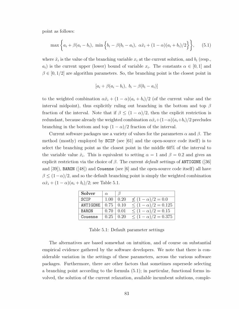
point as follows:

max

ai + β(ai − bi), min

bi − β(bi − ai), αxi + (1− α)(ai + bi)/2

, (5.1)

where xi is the value of the branching variable xi at the current solution, and bi (resp.,

ai) is the current upper (lower) bound of variable xi. The constants α ∈ [0, 1] and

β ∈ [0, 1/2] are algorithm parameters. So, the branching point is the closest point in

[ai + β(ai − bi), bi − β(bi − ai)]

to the weighted combination αxi + (1 − α)(ai + bi)/2 (of the current value and the

interval midpoint), thus explicitly ruling out branching in the bottom and top β

fraction of the interval. Note that if β ≤ (1 − α)/2, then the explicit restriction is

redundant, because already the weighted combination αxi+(1−α)(ai+bi)/2 precludes

branching in the bottom and top (1− α)/2 fraction of the interval.

Current software packages use a variety of values for the parameters α and β. The

method (mostly) employed by SCIP (see [61] and the open-source code itself) is to

select the branching point as the closest point in the middle 60% of the interval to

the variable value xi. This is equivalent to setting α = 1 and β = 0.2 and gives an

explicit restriction via the choice of β. The current default settings of ANTIGONE ([36]

and [39]), BARON ([48]) and Couenne (see [6] and the open-source code itself) all have

β ≤ (1−α)/2, and so the default branching point is simply the weighted combination

αxi + (1− α)(ai + bi)/2; see Table 5.1.

Solver α βSCIP 1.00 0.20 6≤ (1− α)/2 = 0.0ANTIGONE 0.75 0.10 ≤ (1− α)/2 = 0.125BARON 0.70 0.01 ≤ (1− α)/2 = 0.15Couenne 0.25 0.20 ≤ (1− α)/2 = 0.375

Table 5.1: Default parameter settings

The alternatives are based somewhat on intuition, and of course on substantial

empirical evidence gathered by the software developers. We note that there is con-

siderable variation in the settings of these parameters, across the various software

packages. Furthermore, there are other factors that sometimes supersede selecting

a branching point according to the formula (5.1); in particular, functional forms in-

volved, the solution of the current relaxation, available incumbent solutions, comple-

83

mentarity considerations, etc. Our work in this chapter is based solely on analyzing

the volumes of relaxations for triple products, with the goal of helping to inform and

in some cases mathematically support the choice of a branching point.

5.3 Results

In this section, and as we have been doing throughout, we focus on trilinear

monomials. As before, for the variables xi ∈ [ai, bi], i = 1, 2, 3, we assume that the

following conditions hold:

0 ≤ ai < bi for i = 1, 2, 3, and

a1b2b3 + b1a2a3 ≤ b1a2b3 + a1b2a3 ≤ b1b2a3 + a1a2b3,(Ω)

We also recall that because we are only considering non-negative bounds, the

latter part of Ω is equivalent to:

a1b1≤ a2b2≤ a3b3.

Consider what happens when we pick a branching variable, and branch at a given

point: we obtain two subproblems, now with different bounds on the branching vari-

able. The upper bound of the branching variable in the left subproblem becomes the

value of the branching point, as does the lower bound of the branching variable in

the right subproblem. We reconvexify the two subproblems using our chosen method

of convexification (i.e. the full hull or a double McCormick), and we can sum the

volumes from both subproblems to obtain the total volume when branching at that

given point. We are interested in finding the branching point that leads to the least

total volume. For an example of this principle in a lower dimension see Figure 1.2,

which illustrates reconvexifying after branching in sBB. In the context of this dia-

gram, we wish to find the branching point that minimizes the sum of the areas of the

two green regions. Clearly this depends on the choice of convexification method.

Throughout this section, we focus on what happens when we branch on variable

x1. We chose to analyze x1 because some early investigation suggested that branching

on this variable (given that we branch at an optimal point) may result in the least

total volume when compared with branching on x2 or x3. This intuition is merely

based on partial results; however, we do believe that following this work on x1, it

will also be possible to complete the analysis of branching on variable x2 and variable

x3. For the convex-hull convexification, we can see from the structure of the volume

84

function (see Theorem 3.1), that once the analysis has been completed for one of the

variables x2 or x3, completing the last one will be trivial.

We can compute the volume of the relaxation for each of the subproblems using

the appropriate theorem from Chapter 3. To ensure that we compute the appropriate

volumes, we need to check that as the bounds on the branching variable change, we

still respect the labeling Ω. To illustrate this, consider the left subproblem obtained

by branching on variable x1 at some point c1 ∈ [a1, b1]. For this left subproblem, the

lower bound on the branching variable remains the same and the new upper bound is

c1. Intuitively, we can see that if c1 is ‘close’ to b1, then Ω will likely remain satisfied,

however as c1 becomes smaller, there comes a point where eventually the labeling

must change. By simple algebra, we calculate that this critical point is at c1 = a1b2a2

(assuming for now that a2 > 0). We can think about the right subproblem in the

same manner. On the right, the upper bound on the branching variable remains the

same, and the new lower bound is c1. When c1 is close to a1, Ω will likely remain

satisfied, however, as c1 becomes larger, eventually the labeling must change. This

critical point for the right subproblem is at c1 = b1a2b2

.

Therefore, it is natural to think about two cases. First when

b1a2b2≤ a1b2

a2⇐⇒ a22

b22≤ a1b1

⇐⇒ b1a22 ≤ a1b

22,

and second when

b1a2b2

>a1b2a2

⇐⇒ a22b22>a1b1

⇐⇒ b1a22 > a1b

22.

The case of equality, i.e., b1a2b2

= a1b2a2

, is arbitrarily included with Case 1. In fact, when

equality holds, the analysis that follows in the remainder of this chapter is simplified

and it could be contained in either of the cases.

For an illustration of when the labeling must change on one or both of the intervals

to ensure that Ω remains satisfied see Figure 5.2. Finally, we note that we must

consider separately what happens when a2 = 0 because when this happens our case

analysis involves division by zero.

5.3.1 The convex-hull convexification

In this section, we assume that the convexification used is the full convex hull.

We note that because of the structure of the volume function of the convex hull, (see

Theorem 3.1), the second and third variables are interchangeable. This means that

85

Figure 5.1: Variable labeling as the branching point varies in Case 0

(a) Case 1

(b) Case 2

Figure 5.2: Variable labeling as the branching point varies in Case 1 and Case 2

we do not need to consider what happens when the bounds vary enough for x1 to be

relabeled as x3. We complete the analysis by considering the two cases described in

the previous section, however, we first briefly deal with the a2 = 0 case.

5.3.1.1 Case 0: a2 = 0

From the condition Ω, we know that a2 = 0 ⇒ a1 = 0. In this special case,

the labeling for the left subproblem does not change no matter how small the upper

bound becomes. Conversely, the labeling for the right subproblem changes as soon

86

as the lower bound becomes positive. We therefore have the picture shown in Figure

5.1, and only one function to consider over the entire domain, [a1, b1]. As we will see

shortly, this function is a convex quadratic, and therefore it is easy to check that in

this special case the minimizer of this function (later defined as q3), is the midpoint

of the interval.

5.3.1.2 Case 1: b1a2b2≤ a1b2

a2

We define

V (l1, u1, l2, u2, l3, u3) : = (u1 − l1)(u2 − l2)(u3 − l3)× (u1(5u2u3− l2u3 − u2l3 − 3l2l3) + l1(5l2l3 − u2l3 − l2u3 − 3u2u3)) /24

to be the volume of the convex hull with variable lower bounds li and upper bounds,

ui, for i = 1 . . . 3.

Then, for a given problem with initial upper and lower bounds (a1, b1, a2, b2, a3,

b3), the total volume of the two subproblems after branching at point c1, is given by

the following parameterized function:

(5.2)TV (c1) : =

V1(c1) a1 ≤ c1 ≤ b1a2

b2;

V2(c1)b1a2b2≤ c1 ≤ a1b2

a2;

V3(c1)a1b2a2≤ c1 ≤ b1,

where:

V1(c1) := V (a2, b2, a1, c1, a3, b3) + V (c1, b1, a2, b2, a3, b3),

V2(c1) := V (a2, b2, a1, c1, a3, b3) + V (a2, b2, c1, b1, a3, b3),

V3(c1) := V (a1, c1, a2, b2, a3, b3) + V (a2, b2, c1, b1, a3, b3).

This is a piecewise-quadratic function in c1. It is straightforward to check that the

function is continuous over its domain. Furthermore, by observing that the leading

coefficient of each piece is non-negative for all parameter values satisfying Ω, we

conclude that each piece is convex.

The leading coefficient of V1(c1) is:(b3 − a3)(b2 − a2)(8b2b3 − 6a2a3 − 2a2b3)

24≥ 0.

The leading coefficient of V2(c1) is:

(b3 − a3)(b2 − a2)(6b2b3 + 2b2a3 − 6a2a3 − 2a2b3)

24≥ 0.

87

The leading coefficient of V3(c1) is:(b3 − a3)(b2 − a2)(6b2b3 + 2b2a3 − 8a2a3)

24≥ 0.

Figure 5.3 gives some intuition of what this function could look like.

Figure 5.3: Illustration of a continuous piecewise-quadratic function

Now that we know that TV (c1) has this structure, to find the minimizer over the

domain [a1, b1], we can simply find the minimizer on each of the three pieces and

pick the point with the least function value. Because we have convex functions, the

minimum of a given piece will either occur at the global minimizer of the function

(if this occurs over the appropriate subdomain), or at one of the end points of the

subdomain. Therefore, to find the minimizer for a given segment, we first find the

minimizer of the function over the entire real line and check if it occurs in the interval;

if so, it is the minimizer, if not, we examine the interval end points to obtain the

minimizer. We can then compare the function value of the minimizer of each of the

three pieces to find the minimizer of TV (c1), i.e., the branching point that obtains

the least total volume.

We compute the following:

The minimum of V1(c1) occurs at:

c1 =3a1a2a3 + a1a2b3 − a1b2a3 − 3a1b2b3 + 4b1a2a3 − 4b1b2b3

2(3a2a3 + a2b3 − 4b2b3)=: q1.


c1 =a1 + b1

2=: q2.

88


c1 =4a1a2a3 − 4a1b2b3 + 3b1a2a3 + b1a2b3 − b1b2a3 − 3b1b2b3

2(4a2a3 − b2a3 − 3b2b3)=: q3.

Therefore, the candidate points for the minimizer are a1,b1a2b2

, a1b2a2

, b1, q1, q2 and

q3. We can immediately discard a1 and b1 because these are both equivalent to not

branching. By branching and reconvexifying over the two subproblems, we can never

do worse with regard to volume. Therefore, we have five points to consider. For a

given set of parameters, it is straightforward to evaluate and check which of these five

points is the minimizer. However, making use of the following observations, we can

further reduce the possibilities.

If q1 were to be the global minimizer, then it must fall in the appropriate subdo-

main, i.e., it must be that q1 ≤ b1a2b2

. However, by Lemma 5.8 (see §5.5), in Case 1

we always have q1 ≥ b1a2b2

. Therefore, we can discard q1 as a candidate point for the

minimizer because for it to be the minimizer this quantity would have to be exactly

equal to b1a2b2

, which is already on the list of candidate points.

Now, consider the quantities:

q1 −a1 + b1

2=

(b3 − a3)(b1a2 − a1b2)2(4b2b3 − a2b3 − 3a2a3)

≥ 0, (5.3)

and

q3 −a1 + b1

2=

(a3 − b3)(b1a2 − a1b2)2(3b2b3 + b2a3 − 4a2a3)

≤ 0. (5.4)

We therefore have:

q1 ≥ q2 =a1 + b1

2≥ q3. (5.5)

From this, we can observe that if q3 ≥ a1b2a2

, then q2 ≥ q3 ≥ a1b2a2

, and therefore q3 is

the minimizer. This is because neither q1 nor q2 fall in their key intervals; furthermore,

by definition of q3 as the minimizer of V3, we must have that V3(q3) ≤ V3

(a1b2a2

), and

by Lemma 5.5 (see §5.5) we know that V3

(a1b2a2

)≤ V2

(b1a2b2

).

If this does not occur, i.e. q3 <a1b2a2

, then if b1a2b2≤ a1+b1

2≤ a1b2

a2, the midpoint q2 is

the minimizer. This is because under these conditions, q2 is the only minimizer that

occurs in the ‘correct’ function piece, and by definition of q2 as the minimizer of V2,

the function value is not more than at either of the end points.

Otherwise, if none of the above occurs (i.e., none of the intervals contain their

function global minimizer), we have that a1b2a2

is the minimizer by Lemma 5.5 (see

§5.5).

89

As an interesting side point, we also note that if it were possible to have q1 ≤ b1a2b2

,

then q3 ≤ q2 ≤ q1 ≤ b1a2b2

, and therefore q1 would be the minimizer. This is because

neither q2 nor q3 would fall in their key intervals; furthermore, by definition of q1 as

the minimizer of V1, we have that V1(q1) ≤ V1

(b1a2b2

), and by Proposition 5.4 (see

§5.5) we know that V1(q1) ≤ V2

(a1b2a2

). However, by Lemma 5.8 (see §5.5) we have

already discarded this case.

5.3.1.3 Case 2: b1a2b2

> a1b2a2

In this second case, for a given problem with initial upper and lower bounds (a1,

b1, a2, b2, a3, b3), the total volume of the two subproblems after branching at point

c1, is given by the following parameterized function (this is similar, but distinct, from

the function in Case 1):

(5.6)T V (c1) : =

V1(c1) a1 ≤ c1 ≤ b1a2

b2;

V4(c1)b1a2b2≤ c1 ≤ a1b2

a2;

V3(c1)a1b2a2≤ c1 ≤ b1,

where V1(c1) and V3(c1) are defined as before and:

V4(c1) := V (a1, c1, a2, b2, a3, b3) + V (c1, b1, a2, b2, a3, b3).

Again, this is a piecewise-quadratic function in c1, and it is simple to check that the

function is continuous over its domain. Furthermore, by observing that the leading

coefficient of each piece is non-negative for all parameter values satisfying Ω, we know

that each piece is convex.

The leading coefficient of V4(c1) is:(b3 − a3)(b2 − a2)(8b2b3 − 8a2a3)

24≥ 0.

Therefore, we can take the same approach as before to find the minimizer: first

find the minimizer for each segment. We do this by finding the minimizer for the

appropriate function over the whole real line and checking if it occurs in the segment.

If it does, we have found the minimizer for that segment, if not, we examine the

interval end points. We then compare the minimum in each of the three sections to

find the branching point that obtains the least volume.

From our analysis of Case 1, we know that the minimums of V1(c1) and V3(c1)

occur at q1 and q3 respectively. We compute that the minimum of V4(c1) occurs at

90

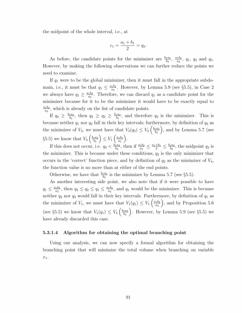
the midpoint of the whole interval, i.e., at

c1 =a1 + b1

2= q2.

As before, the candidate points for the minimizer are b1a2b2

, a1b2a2

, q1, q2 and q3.

However, by making the following observations we can further reduce the points we

need to examine.

If q1 were to be the global minimizer, then it must fall in the appropriate subdo-

main, i.e., it must be that q1 ≤ a1b2a2

. However, by Lemma 5.9 (see §5.5), in Case 2

we always have q1 ≥ a1b2a2

. Therefore, we can discard q1 as a candidate point for the

minimizer because for it to be the minimizer it would have to be exactly equal toa1b2a2

, which is already on the list of candidate points.

If q3 ≥ b1a2b2

, then q2 ≥ q3 ≥ b1a2b2

, and therefore q3 is the minimizer. This is

because neither q1 nor q2 fall in their key intervals; furthermore, by definition of q3 as

the minimizer of V3, we must have that V3(q3) ≤ V3

(b1a2b2

), and by Lemma 5.7 (see

§5.5) we know that V3

(b1a2b2

)≤ V1

(a1b2a2

).

If this does not occur, i.e. q3 <b1a2b2

, then if a1b2a2≤ a1+b1

2≤ b1a2

b2, the midpoint q2 is

the minimizer. This is because under these conditions, q2 is the only minimizer that

occurs in the ‘correct’ function piece, and by definition of q2 as the minimizer of V4,

the function value is no more than at either of the end points.

Otherwise, we have that b1a2b2

is the minimizer by Lemma 5.7 (see §5.5).

As another interesting side point, we also note that if it were possible to have

q1 ≤ a1b2a2

, then q3 ≤ q2 ≤ q1 ≤ a1b2a2

, and q1 would be the minimizer. This is because

neither q2 nor q3 would fall in their key intervals. Furthermore, by definition of q1 as

the minimizer of V1, we must have that V1(q1) ≤ V1

(a1b2a2

), and by Proposition 5.6

(see §5.5) we know that V1(q1) ≤ V4

(b1a2b2

). However, by Lemma 5.9 (see §5.5) we

have already discarded this case.

5.3.1.4 Algorithm for obtaining the optimal branching point

Using our analysis, we can now specify a formal algorithm for obtaining the

branching point that will minimize the total volume when branching on variable

x1.

91

Data: (a1, b1, a2, b2, a3, b3)

Result: Branching point for variable x1 resulting in least total volume

1 initialization

2 q2 := a1+b12

3 q3 := 4a1a2a3−4a1b2b3+3b1a2a3+b1a2b3−b1b2a3−3b1b2b32(4a2a3−b2a3−3b2b3)

4 if a2 = 0 then // Case 0 (see §5.3.1.1)5 return q3(= q2)

6 end

7 else

8 if a1b2a2≥ b1a2

b2then // Case 1 (see §5.3.1.2)

9 if q3 ≥ a1b2a2

then

10 return q3

11 end

12 else if q2 ≥ b1a2b2

and q2 ≤ a1b2a2

then

13 return q2

14 else

15 return a1b2a2

16

17 end

18 else // Case 2 (see §5.3.1.3)19 if q3 ≥ b1a2

b2then

20 return q3

21 end

22 else if q2 ≥ a1b2a2

and q2 ≤ b1a2b2

then

23 return q2

24 else

25 return b1a2b2

26

27 end

28 endAlgorithm 1: Optimal branching point for x1

5.3.1.5 Some examples

We can illustrate these piecewise-quadratic functions for the possible outcomes of

Algorithm 1. In this illustration, we focus on Case 1, and therefore Figure 5.4 shows

92

the function TV (c1) over the domain [a1, b1]. The red curve illustrates an example

where the minimizer of V3(c1), (i.e. q3), falls in the relevant interval, and therefore is

the minimizer over our whole domain. The blue curve illustrates an example where q3

does not fall in this interval, however the midpoint, q2, falls in between the quantitiesb1a2b2

and a1b2a2

and is therefore the required minimizer. The green curve illustrates an

example where neither of the above happens, and therefore the breakpoint between

the function V2(c1) and the function V3(c1) is the minimizer. In this example we are

in Case 1, and therefore this point is a1b2a2

.

Figure 5.4: Picture to illustrate the possible outcomes of Algorithm 1 in Case 1

It is important to note that each of the cases in Algorithm 1 actually can occur.

Unfortunately, the plots of the ‘real’ functions do not display the key details as clearly

as our illustration, so we do not include them here. However, it is easy to check the

following:

• An example of a red curve (minimum occurs at q3) is (a1 = 1, b1 = 35, a2 = 2,

93

b2 = 12, a3 = 12, b3 = 35).

• An example of a blue curve (minimum occurs at q2) is (a1 = 1, b1 = 34, a2 = 2,

b2 = 35, a3 = 12, b3 = 35).

• An example of a green curve (minimum occurs at a1b2a2

) is (a1 = 1, b1 = 8,

a2 = 5, b2 = 22, a3 = 1, b3 = 4).

Furthermore, an example of Case 2, where the minimum occurs at the breakpoint

between the function V4 and the function V3, i.e. the point b1a2b2

is (a1 = 1, b1 = 13,

a2 = 1, b2 = 2, a3 = 2, b3 = 4). Finally, a simple example of Case 0, is the special

case (a1 = 0, b1 = 1, a2 = 0, b2 = 1, a3 = 0, b3 = 1). In Figure 5.5 we can see the plot

of this function and the minimum, which falls at the midpoint. In Case 0 we always

have q1 = q2 = q3 = a1+b12

.

0 0.1 0.2 0.3 0.4 0.5 0.6 0.7 0.8 0.9 1

0.15

0.16

0.17

0.18

0.19

0.2

0.21

Figure 5.5: Plot of the total volume function for parameter values:(a1 = 0, b1 = 1, a2 = 0, b2 = 1, a3 = 0, b3 = 1)

5.3.1.6 Global convexity of our piecewise-quadratic function over its do-

main

We have seen that each piece of TV (c1) and T V (c1) is a convex quadratic function.

However, this does not imply that the functions are convex over the whole domain,

94

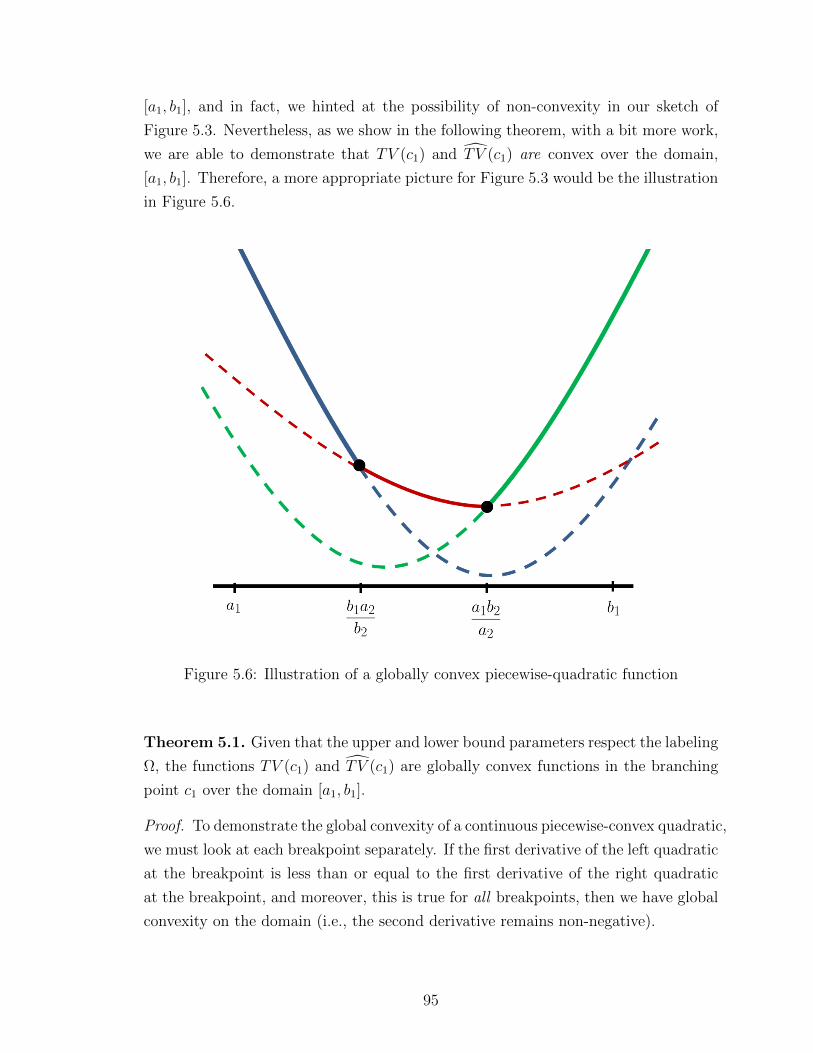
[a1, b1], and in fact, we hinted at the possibility of non-convexity in our sketch of

Figure 5.3. Nevertheless, as we show in the following theorem, with a bit more work,

we are able to demonstrate that TV (c1) and T V (c1) are convex over the domain,

[a1, b1]. Therefore, a more appropriate picture for Figure 5.3 would be the illustration

in Figure 5.6.

Figure 5.6: Illustration of a globally convex piecewise-quadratic function

Theorem 5.1. Given that the upper and lower bound parameters respect the labeling

Ω, the functions TV (c1) and T V (c1) are globally convex functions in the branching

point c1 over the domain [a1, b1].

Proof. To demonstrate the global convexity of a continuous piecewise-convex quadratic,

we must look at each breakpoint separately. If the first derivative of the left quadratic

at the breakpoint is less than or equal to the first derivative of the right quadratic

at the breakpoint, and moreover, this is true for all breakpoints, then we have global

convexity on the domain (i.e., the second derivative remains non-negative).

95

The functions TV (c1) and T V (c1) are both continuous on [a1, b1]. Furthermore,

they each have two breakpoints: one at b1a2b2

, and the other at a1b2a2

. Therefore, to

demonstrate global convexity over [a1, b1] for each function, we have two breakpoints

to consider in each case.

Global convexity of TV (c1): First, we compare the first derivatives of V1 and

V2 at the breakpoint b1a2b2

:

dV2dc1

(b1a2b2

)− dV1dc1

(b1a2b2

)=

1

12b1(b3 − a3)2(b2 − a2)2 ≥ 0.

Secondly, we compare the first derivatives of V2 and V3 at breakpoint a1b2a2

:

dV3dc1

(a1b2a2

)− dV2dc1

(a1b2a2

)=

1

12a1(b3 − a3)2(b2 − a2)2 ≥ 0.

These quantities are both non-negative; therefore, we observe that TV (c1) is glob-

ally convex over the domain [a1, b1].

Global convexity of T V (c1): First, we compare the first derivatives of V1 and

V4 at the breakpoint a1b2a2

:

dV4dc1

(a1b2a2

)− dV1dc1

(a1b2a2

)=

1

12a1(b3 − a3)2(b2 − a2)2 ≥ 0.

Secondly, we compare the first derivatives of V4 and V3 at the breakpoint b1a2b2

:

dV3dc1

(b1a2b2

)− dV4dc1

(b1a2b2

)=

1

12b1(b3 − a3)2(b2 − a2)2 ≥ 0

These quantities are both non-negative; therefore, we observe that T V (c1) is also

globally convex over the domain [a1, b1].

5.3.1.7 Bounds on where the optimal branching point can occur

We have seen in §5.2 that software employ methods to avoid selecting a branching

point that falls too close to either endpoint of the interval. Therefore, a natural issue

to consider is whether this minimizer can fall close to either of the endpoints. We want

to know how likely it is that solvers are routinely precluding the “best” branching

point. The following propositions give some insight to this issue and show that, in

fact, software is unlikely to be cutting off the optimal branching point.

96

Proposition 5.2. The branching point for variable x1 that obtains the least volume,

never occurs at a point in the interval greater than the midpoint.

Proof. If a2 = 0, then we are in Case 0, and the minimizer is at the midpoint, which

is clearly no greater than the midpoint.

If a1b2a2≥ b1a2

b2, then we are in Case 1. If q3 ≥ a1b2

a2, then q3 is the minimizer, but

we know that q3 ≤ a1+b12

(see 5.4). If q2 = a1+b12

falls in the interval[b1a2b2, a1b2a2

],

then the midpoint is the minimizer. If it does not, then (i) a1b2a2

is the minimizer,

and (ii) it must be that either that a1+b12

> a1b2a2

, in which case our claim is valid, ora1+b1

2< b1a2

b2≤ a1b2

a2. We will show by contradiction that this cannot be the case.

For contradiction assume that:

a1 + b12

<b1a2b2

anda1 + b1

2<a1b2a2

.

This implies:

2b1a2 − b1b2 − a1b2 = b1(a2 − b2) + (b1a2 − a1b2) > 0, and

2a1b2 − a1a2 − b1a2 = a1(b2 − a2) + (a1b2 − b1a2) > 0.

Now let X := b2−a2 and Y := b1a2−a1b2 (note that both X and Y are non-negative).

Therefore we can write our assumption as:

b1(−X) + Y > 0 and a1(X) + (−Y ) > 0,

which implies

Y > b1X and Y < a1X,

a contradiction. Therefore, in Case 1 the minimizer must be no larger than the

midpoint.

We make a similar argument for Case 2. Here a1b2a2

< b1a2b2

. If q3 ≥ b1a2b2

, then q3

is the minimizer, but we know that q3 ≤ a1+b12

(see 5.4). If q2 = a1+b12

falls in the

interval[a1b2a2, b1a2b2

], then the midpoint is the minimizer. If it does not, then (i) b1a2

b2

is the minimizer, and (ii) it must be that either that a1+b12

> b1a2b2

, in which case our

claim is valid, or a1+b12

< a1b2a2

< b1a2b2

. However, we have just shown by contradiction

that this cannot be the case. Therefore, in Case 2 the minimizer must be no larger

than the midpoint.

97

This proposition gives an upper bound on the fraction through the interval the

minimizer can fall (namely 12). Furthermore, this bound is sharp, given that we know

examples when the minimizer is exactly at the midpoint. It would be nice to also

obtain a sharp lower bound on this fraction. By demonstrating that the minimizer

cannot fall too close to the end points of the interval, we are providing evidence

to back up software’s current choice of branching point, as discussed in §5.2. The

following proposition gives a lower bound on this fraction when a2 6= 0, (when a2 = 0,

we know that the minimizer will be exactly at the midpoint).

Proposition 5.3. Given upper and lower bound parameters (a1, b1, a2, b2, a3, b3)

satisfying Ω, and a2 6= 0. The branching point for variable x1 that obtains the least

volume, never occurs at a point in the interval less than

min

max

a1(b2 − a2)a2(b1 − a1)

,b1a2 − a1b2b1b2 − a1b2

,1

2

of the way through the interval.

Proof. There are four candidate points where the minimizer can occur. Namely,

q2 = a1+b12

, q3,a1b2a2

, and b1a2b2

. Therefore

min

a1 + b1

2, q3,

a1b2a2

,b1a2b2

,

is a trivial lower bound on this minimizer.

We know that if q3 is the minimizer, then we must have q3 ≥ a1b2a2

(Case 1), or

q3 ≥ b1a2b2

(Case 2), so we can discard this point.

Additionally, we know that if a1b2a2

is the minimizer, then we have a1b2a2≥ b1a2

b2(Case

1), and if b1a2b2

is the minimizer, then we have b1a2b2

> a1b2a2

(Case 2).

Therefore we have that a lower bound on the minimizer is:

min

max

a1b2a2

,b1a2b2

,a1 + b1

2

.

Moreover, a lower bound for the fraction of the interval where this point can fall is:

min

max

a1b2a2− a1

b1 − a1,b1a2b2− a1

b1 − a1

,a1+b1

2− a1

b1 − a1

= min

max

a1(b2 − a2)a2(b1 − a1)

,b1a2 − a1b2b1b2 − a1b2

,1

2

.

98

We note that this lower bound is unlikely to be sharp. Consider the case where

a1 = 0, a2 = ε > 0 and b2 = 1. This bound becomes ε, and is therefore not particularly

informative, given that we can make ε as close to zero as we wish. However, we have

checked millions of examples and are yet to find an example where the minimizer

occurs less than ∼ 0.45 of the way through the interval. It would be nice to sharpen

this bound, and our computations indicate that this should be possible.

5.3.2 The best double-McCormick convexification

Unlike ANTIGONE ([37]) and BARON ([49]), some software does not use the explicit

convex hull for trilinear monomials, but instead employs repeated McCormick convex-

ifications to obtain a relaxation; see SCIP ([61]) and Couenne ([6]). Here, we describe

some partial branching-point analysis for the best double-McCormick relaxation P3

(the relaxation with the least volume). We do note that currently SCIP and Couenne

do not always use P3; rather, their choice of which double McCormick is arbitrary.

However, because of our results from Chapter 3, we choose to focus on P3. As we did

in §5.3.1, we assume throughout that we branch on variable x1.

When analyzing the branching point for the double-McCormick convexification,

it is important to note that variables x2 and x3 are not interchangeable. This is

because of the structure of the volume function of P3 (see Theorem 3.4). This means

that we do need to consider the what happens when the bounds of x1 vary enough

for x1 to be relabeled as x3, and the case analysis becomes more complicated than

in the convex-hull analysis. The original Case 1 (recall Figure 5.2) splits into three

further cases, while Case 2 remains as only one case. The number of pieces of the

piecewise functions increase for all cases. See Figure 5.7 for an illustration (as before,

the a3 = 0 and/or a2 = 0 cases will need to be handled separately).

99

(a) Case 1a

(b) Case 1b

(c) Case 1c

(d) Case 2

Figure 5.7: Case analysis for P3

100

It is clear that the for the double-McCormick convexification, even when only

considering the case analysis, the situation is much more complex. We would like to

perform the same analysis that we did for the convex-hull case. Namely: construct

the appropriate piecewise functions for each case; establish the convexity of each piece

(for each case); find a closed form expression for the global minimizer of each piece.

Using this information, we would then be able to specify an algorithm to: (i) check

if the global minimizer falls in the appropriate segment of the interval, and if not,

check the end points to find the minimizer over that segment and then (ii) compare

the minimums of each segment to find the global minimizer. This could be done for

each case.

However, because in this section we present only a partial analysis, we will focus

on the segment where the branching point is such that none of the variables need to

be relabeled. This is the middle segment of Case 2. We define the relevant function

for this segment of the interval, and note that it is no longer a quadratic. However,

we are able to establish that it is convex, and therefore for a given problem we will be

able to efficiently calculate the minimizer (and minimum). Unfortunately, in general,

we are unable to get a closed-form expression for the minimizer, but with a bit of

work, we are able to obtain a rather small window for where the minimum will occur.

To begin, we define

VDM(l1, u1, l2, u2, l3, u3) : =

((u1 − l1)(u2 − l2)(u3 − l3)

× (u1(5u2u3 − l2u3 − u2l3 − 3l2l3) + l1(5l2l3 − u2l3 − l2u3 − 3u2u3))

24

)

+(u1 − l1)(u2 − l2)2(u3 − l3)2 (5(l1u1u2 − l1u1l2) + 3(u21l2 − l21u2))

24(u1u2 − l1l2),

to be the volume of the relaxation P3, with variable lower bounds li and upper

bounds, ui, for i = 1 . . . 3.

Then, for a given problem with initial upper and lower bounds (a1, b1, a2, b2, a3,

b3), the total volume of the two subproblems after branching at point c1 (given that

we have a1b2a2≤ c1 ≤ b1a2

b2), is described by the following parameterized function:

TVDM(c1) = VDM(a1, c1, a2, b2, a3, b3) + VDM(c1, b1, a2, b2, a3, b3).

This function is not a quadratic, but it is convex. See Theorem 5.10 (§5.5) for the

proof of convexity.

101

As noted, we are unable to obtain a closed form expression for the minimizer of

this function, but we are able to obtain a small window for where the minimum will

occur. In particular, we establish that the minimizer must be strictly greater than

the midpoint. For this proof see Proposition 5.11 (§5.5). We also establish that the

furthest right this minimizer can occur is 1/√

3 ≈ 0.5773503 of the way through the

interval. For this proof see Theorem 5.12 (§5.5).

Furthermore, we can find examples where the minimum occurs very close to the

midpoint of the interval. For example, with ai = 1000, bi = 1001, for all i, the

minimum occurs at c1 ≈ 1000.500008. We can also find examples where the minimum

occurs exactly 1/√

3 of the way through the interval. For the special case of ai = 0

and bi = 1 for i = 1, 2, 3, we find that the minimum of the function is obtained when

branching at c1 = 1/√

3 ≈ 0.5773503. Therefore, our result that the minimizer occurs

somewhere between 0.5 of the way and 1/√

3 ≈ 0.5773503 of the way through the

interval is essentially sharp.

By identifying and analyzing the appropriate piecewise functions for the other

possible cases described by Figure 5.7, we expect to be able to obtain an algorithm,

in the spirit of Algorithm 1, that would output the optimal branching point for x1

when using the relaxation P3.


In this section we have produced a simple algorithm for obtaining the optimal

branching point when using the convex-hull convexification and branching on vari-

able x1. We have provided a sharp upper bound on where in the interval the minimizer

can occur, and we have also obtained a lower bound for this fraction. We have compu-

tational evidence to suggest that this lower bound can be sharpened, thus providing

analysis that backs up software’s current choice of branching point. Furthermore,

we have shown that the piecewise-quadratic functions we have been considering are

globally convex over their entire domain.

We have begun the analysis for obtaining the optimal branching point when using

the best double-McCormick convexification and branching on variable x1, but this

case is far more complex. Alongside completing the double-McCormick analysis for

x1, it would be a natural next step to obtain results for branching on x2 or x3 using

either convexification.

102

5.5 Technical propositions, lemmas, and theorems

In this section we state the propositions, lemmas, and theorems used for the

analysis, along with their proofs.

5.5.1 Convex-hull convexification

Proposition 5.4. Given that the upper and lower bound parameters respect the

labeling Ω, and b1a2b2≤ a1b2

a2,

V1(q1) ≤ V2

(a1b2a2

)= V3

(a1b2a2

).

Proof. It is easy to check that V2

(a1b2a2

)= V3

(a1b2a2

).

V2

(a1b2a2

)− V1(q1) =

(b3 − a3)(b2 − a2)48(4b2b3 − a2b3 − 3a2a3)a22

×(pa21 + qa1 + r

),

where

p =(− 3a2a3 − a2b3 + b2a3 + 3b2b3

)×(

− 3a32a3 − a32b3 + 13a22b2a3 + 7a22b2b3 − 12a2b22a3 − 20a2b

22b3 + 16b32b3

)=(− 3a2a3 − a2b3 + b2a3 + 3b2b3

)×(

(−3a32 + 13a22b2 − 12a2b22)a3 + (−a32 + 7a22b2 − 20a2b

22 + 16b32)b3

),

q = 4a2b1(2a22a3 − 3a2b2a3 − 3a2b2b3 + 4b22b3)(3a2a3 + a2b3 − b2a3 − 3b2b3),

r = 4a22b21(a2a3 + a2b3 − 2b2b3)

2.

To show that V2

(a1b2a2

)− V1(q1) is non-negative for all parameters satisfying Ω,

we will show that pa21 + qa1 + r ≥ 0 for all parameters satisfying Ω.

We observe:((−a32 + 7a22b2 − 20a2b

22 + 16b32)b3 + (−3a32 + 13a22b2 − 12a2b

22)a3

)=: b3Y + a3Z,

where

Y + Z = 4(b2 − a2)(2b2 − a2)2 ≥ 0,

and

Y =

(b2 − a2

)(4b2(b2 − a2) + 12b22 + a22

)+ 2a22b2 ≥ 0.

103

Therefore, by Lemma 3.12 we have that b3Y + a3Z is non-negative and so p is

non-negative. From this we know that pa21 + qa1 + r is a convex function in a1 and

we can find the minimizer by setting the derivative to zero and solving for a1. The

minimum occurs at

a1 =2b1a2(2a

22a3 − 3a2b2a3 − 3a2b2b3 + 4b22b3)

(−3a32a3 − a32b3 + 13a22b2a3 + 7a22b2b3 − 12a2b22a3 − 20a2b22b3 + 16b32b3).

Substituting this in to pa21 + qa1 + r, we obtain that the minimum value of this

quadratic is:

4a22b21(b3 − a3)(b2 − a2)3(3a2a3 + a2b3 − 4b2b3)

2

(−3a32a3 − a32b3 + 13a22b2a3 + 7a22b2b3 − 12a2b22a3 − 20a2b22b3 + 16b32b3).

We have already shown that the denominator is non-negative, and it is easy to

see that the numerator is non-negative for all values of the parameters satisfying Ω.

Therefore pa21 + qa1 + r ≥ 0, and consequently, V2

(a1b2a2

)− V1(q1) ≥ 0 as required.

Lemma 5.5. Given that the upper and lower bound parameters respect the labeling

Ω, and b1a2b2≤ a1b2

a2,

V1

(b1a2b2

)= V2

(b1a2b2

)≥ V2

(a1b2a2

)= V3

(a1b2a2

)


(b1a2b2

)= V2

(b1a2b2

)and V2

(a1b2a2

)= V3

(a1b2a2

).

Furthermore,

V2

(b1a2b2

)− V2

(a1b2a2

)=

(b3 − a3)(b2 − a2)2(b1a2 − a1b2)(a1b22 − a22b1)(−3a2a3 − a2b3 + b2a3 + 3b2b3)

12a22b22

≥ 0,

as required.


labeling Ω, and b1a2b2

> a1b2a2

,

V1(q1) ≤ V4

(b1a2b2

)= V3

(b1a2b2

).

104


(b1a2b2

)= V3

(b1a2b2

).

V4

(b1a2b2

)− V1(q1) =

(b3 − a3)(b2 − a2)48(4b2b3 − a2b3 − 3a2a3)b22

×(pa21 + qa1 + r

),

where

p = b22(5b2b3 − b2a3 − a2b3 − 3a2a3)2,

q = 8b1b2(6a22a3 + 2a22b3 − 3a2b2a3 − 9a2b2b3 + b22a3 + 3b22b3)(b2b3 − a2a3),

r = 16b21(−3a32a3 − a32b3 + 3a22b2a3 + 5a22b2b3 − a2b22a3 − 4a2b22b3 + b32b3)(b2b3 − a2a3).

To show this is non-negative for all parameters satisfying Ω, we will show pa21 +

qa1 + r ≥ 0 for all parameters satisfying Ω.

Firstly, we observe that

p = b22(5b2b3 − b2a3 − a2b3 − 3a2a3)2 ≥ 0.

From this we know that pa21 + qa1 + r is a convex function in a1, and we can find the

minimizer by setting the derivative to zero and solving for a1. The minimum occurs

at

a1 =4b1(6a

22a3 + 2a22b3 − 3a2b2a3 − 9a2b2b3 + b22a3 + 3b22b3)(a2a3 − b2b3)

b2(3a2a3 + a2b3 + b2a3 − 5b2b3)2.

Substituting this in to pa21 + qa1 + r, we obtain that the minimum value of this

quadratic is:

16b21(b3 − a3)(b2 − a2)3(b2b3 − a2a3)(3a2a3 + a2b3 − 4b2b3)2

(3a2a3 + a2b3 + b2a3 − 5b2b3)2,

which is non-negative for all parameters satisfying Ω. Therefore pa21 + qa1 + r ≥ 0,

and consequently, V4

(b1a2b2

)− V1(q1) ≥ 0, as required.

Lemma 5.7. Given that the upper and lower bound parameters respect the labeling

Ω, and b1a2b2

> a1b2a2

,

V1

(a1b2a2

)= V4

(a1b2a2

)≥ V4

(b1a2b2

)= V3

(b1a2b2

).

105


(a1b2a2

)= V4

(a1b2a2

)and V4

(b1a2b2

)= V3

(b1a2b2

).

Furthermore,

V4

(a1b2a2

)−V4

(b1a2b2

)=

(b3 − a3)(b2 − a2)2(b1a22 − a1b22)(b1a2 − a1b2)(b2b3 − a2a3)3a22b

22

≥ 0,

as required.

Lemma 5.8. Given that the parameters satisfy the conditions Ω, and furthermore,b1a2b2≤ a1b2

a2, we have

q1 ≥b1a2b2

.

Proof. From the proof of Proposition 5.2, we know that the midpoint, q2, cannot be

smaller than both a1b2b1

and b1a2b2

. Therefore we have:

q2 ≥ min

a1b2b1

,b1a2b2

,

and because we saw in 5.5 that q1 ≥ q2 we also have

q1 ≥ min

a1b2b1

,b1a2b2

.

Therefore, under the conditions of the lemma, q1 ≥ b1a2b2

as required.

Lemma 5.9. Given that the parameters satisfy the conditions Ω, and furthermore,b1a2b2≥ a1b2

a2, we have

q1 ≥a1b2a2

.

Proof. We saw in the proof of Lemma 5.8 that

q1 ≥ min

a1b2b1

,b1a2b2

.

Therefore, under the conditions of the lemma, q1 ≥ a1b2a2

as required.

106

5.5.2 Double-McCormick convexification

Theorem 5.10. Given that the upper and lower bound parameters respect the la-

beling Ω, the total volume function:

TVDM(c1) = VDM(a1, c1, a2, b2, a3, b3) + VDM(c1, b1, a2, b2, a3, b3)

is a convex function in the branching point c1, on the domain [a1, b1].

Proof. It is natural to try and show that each summand in the theorem statement is

convex in c1 on the domain [a1, b1]; but this is not the case. Instead, we let

VDM(c1, b1, a2, b2, a3, b3) =: s1 + s2,

and

VDM(a1, c1, a2, b2, a3, b3) =: s3 + s4,

where:

s1 : = (b1 − c1)(b2 − a2)(b3 − a3)×b1(5b2b3 − a2b3 − b2a3 − 3a2a3) + c1(5a2a3 − b2a3 − a2b3 − 3b2b3)

24,

s2 : =(b1 − c1)(b2 − a2)2(b3 − a3)2(3a2b21 − 5a2b1c1 + 5b1b2c1 − 3b2c

21)

24(b1b2 − c1a2),

s3 : = (c1 − a1)(b2 − a2)(b3 − a3)×c1(5b2b3 − a2b3 − b2a3 − 3a2a3) + a1(5a2a3 − b2a3 − a2b3 − 3b2b3)

24,

s4 : =(c1 − a1)(b2 − a2)2(b3 − a3)2(−3a21b2 − 5a1a2c1 + 5a1b2c1 + 3a2c

21)

24(b2c1 − a1a2).

Now, to show that TVDM(c1) = VDM(a1, c1, a2, b2, a3, b3) + VDM(c1, b1, a2, b2, a3, b3) is

convex in c1, we will show that s1 + s2 + s3 is convex in c1, and that s4 is convex in

c1, both over the domain [a1, b1].

Proof of convexity of s1 + s2 + s3

Taking the second derivative of s1 + s2 + s3 with respect to c1 we obtain:

107

(b2 − a2)(b3 − a3)12(b1b2 − c1a2)3

×((8a42a3 + 3a32a3b2 − 11a32b2b3 − 3a22a3b

22 +

3a22b22b3)c

31 + (−24a32a3b1b2 − 9a22a3b1b

22 + 33a22b1b

22b3 + 9a2a3b1b

32 −

9a2b1b32b3)c

21 + (24a22a3b

21b

22 + 9a2a3b

21b

32 − 33a2b

21b

32b3 − 9a3b

21b

42 +

9b21b42b3)c1 + 3a42a3b

31 − 3a42b

31b3 − 11a32a3b

31b2 + 11a32b

31b2b3 +

18a22a3b31b

22 − 18a22b

31b

22b3 − 26a2a3b

31b

32 + 18a2b

31b

32b3 + 8a3b

31b

42

).

It is clear that the first multiplicand is non-negative for all c1 ∈ [a1, b1] (and

parameters satisfying Ω). The second multiplicand is a cubic in c1. By taking the

first derivative of this cubic and setting it equal to zero, we can solve for c1 and

obtain the stationary points. In doing so, we find that there is one repeated root

and therefore one stationary point at c1 = b1b2/a2. Because this cubic has only one

stationary point, we know that it is monotone in c1.

Consider substituting c1 = b1 into this cubic. In doing so, we obtain the quantity

b31(b2 − a2)3 ((b2 + 3a2)(b3 − a3) + 8(b2b3 − a2a3)) ,

which is non-negative for all values of the parameters satisfying Ω.

Substituting c1 = 0 into this cubic, we obtain

b31

(b3(11a32b2+18a2b

32−18a22b

22−3a42)+a3(3a

42+8b42+18a22b

22−26a2b

32−11a32b2)

). (5.7)

We use Lemma 3.12, with:

A = b3,

B = a3,

C = 11a32b2 + 18a2b32 − 18a22b

22 − 3a42 = (18a2b

22 + 3a32)(b2 − a2) + 8a32b2, and

D = 3a42 + 8b42 + 18a22b22 − 26a2b

32 − 11a32b2,

which implies: C+D = 8b32(b2− a2) ≥ 0, to see that 5.7 is non-negative for all values

of the parameters satisfying Ω.

Because the cubic is monotone, we conclude that it is non-negative for all c1 ∈[0, b1] and therefore for all c1 ∈ [a1, b1]. Consequently, the second derivative of s1 +

s2 + s3 with respect to c1 is non-negative on the domain c1 ∈ [a1, b1], and s1 + s2 + s3

is convex.

108

Proof of convexity of s4

Taking the second derivative of s4 with respect to c1 we obtain

(b2 − a2)2(b3 − a3)2

12(c1b2 − a1a2)3×(

(3a2b22)c

31 − (9a1a

22b2)c

21 + (9a21a

32)c1 − 8a31a

32 + 10a31a

22b2 − 8a31a2b

22 + 3a31b

32

).

It is clear that the first multiplicand is non-negative for all c1 ∈ [a1, b1]. The

second multiplicand is a cubic in c1; by taking the first derivative of this cubic and

setting it equal to zero, we can solve for c1 and obtain the stationary points. In

doing so, we find that there is one repeated root and therefore one stationary point

at c1 = a1a2/b2. Because this cubic has only one stationary point, we know that it is

monotone in c1. By considering the leading term of this cubic and seeing that it is

non-negative, we know that this function is non-decreasing.

Substituting c1 = a1 into this cubic, we obtain

a31(3b2 + a2)(b2 − a2)2,

which is non-negative for all values of the parameters satisfying Ω.

Because the cubic is non-decreasing, we conclude that it is non-negative for all

c1 ∈ [a1,∞) and therefore for all c1 ∈ [a1, b1]. Consequently, the second derivative

of s4 with respect to c1 is non-negative over the domain [a1, b1], and therefore s4 is

convex.

Consequently (s1+s2+s3)+s4 = VDM(a1, c1, a2, b2, a3, b3)+VDM(c1, b1, a2, b2, a3, b3)

is a convex function in c1 over the domain [a1, b1] as required.


labeling Ω, the minimum of the convex function

TVDM(c1) = VDM(a1, c1, a2, b2, a3, b3) + VDM(c1, b1, a2, b2, a3, b3)

over the domain c1 ∈ [a1, b1], occurs at some value of c1 > (a1 + b1)/2.

Proof. Consider the value of the first derivative at the midpoint (a1 + b1)/2:

(b1 − a1)3(b2 − a2)3(b3 − a3)2(3a22 − 2a2b2 + 3b22)((a21a2 − b21b2) + 3a1b1(a2 − b2))

24(b1b2 + a1b2 − 2a1a2)2(2b1b2 − a1a2 − b1a2)2.

109

We can see that for all parameters satisfying Ω this quantity is negative (we can claim

negativity and not just non-positivity because we require bi > ai). Therefore at the

midpoint the convex function is still decreasing, and hence the minimum occurs when

c1 > (a1 + b1)/2.

Theorem 5.12. Given that the upper and lower bound parameters respect the la-

beling Ω, the minimum of the convex function

TVDM(c1) = VDM(a1, c1, a2, b2, a3, b3) + VDM(c1, b1, a2, b2, a3, b3),

over the domain c1 ∈ [a1, b1], occurs at some value of c1 ≤ a1+(b1−a1)/√

3. Moreover,

this interval cannot be tightened any further from the right.

Proof. Consider the value of the first derivative at the point c1 = a1 + (b1 − a1)/√

3:

(2√

3− 3)(b1 − a1)(b2 − a2)(b3 − a3)× g12(b2a1

√3− b2

√3b1 + 3a1a2 − 3b2a1)2(a2

√3b1 − b2

√3b1 + 2a1a2 + a2b1 − 3b1b2)2

,

(5.8)

where g is a complicated function of the parameters a1, b1, a2, b2, a3, b3.

We now think of g as a polynomial in a2, parameterized by a1, b1, b2, a3 and b3.

g(a2) = γ5a52 + γ4a

42 + γ3a

32 + γ2a

22 + γ1a2 + γ0,

where:

γ5 :=

(− 54√

3a31a3b1 + 6√

3a31b1b3 + 9√

3a21a3b21 − 33

√3a21b

21b3

− 63√

3a1a3b31 + 63

√3a1b

31b3 − 54a41a3 + 6a41b3 − 54a31a3b1

+ 6a31b1b3 − 48a21b21b3 − 108a1a3b

31 + 108a1b

31b3

),

γ4 :=

(− 24√

3a41a3b2 − 8√

3a41b2b3 + 120√

3a31a3b1b2 + 72√

3a31b1b2b3

+ 3√

3a21a3b21b2 + 165

√3a21b

21b2b3 + 273

√3a1a3b

31b2 − 241

√3a1b

31b2b3

+ 24√

3a3b41b2 − 24

√3b41b2b3 + 78a41a3b2 + 66a41b2b3

+ 156a31a3b1b2 + 36a31b1b2b3 + 54a21a3b21b2 + 282a21b

21b2b3

+ 462a1a3b31b2 − 414a1b

31b2b3 + 42a3b

41b2 − 42b41b2b3

),

110

γ3 :=

(− 8√

3a41a3b22 + 72

√3a41b

22b3 + 40

√3a31a3b1b

22 − 248

√3a31b1b

22b3

+ 78√

3a21a3b21b

22 − 486

√3a21b

21b

22b3 − 526

√3a1a3b

31b

22

+ 366√

3a1b31b

22b3 − 88

√3a3b

41b

22 + 80

√3b41b

22b3 + 14a41a3b

22

− 174a41b22b3 − 128a31a3b1b

22 − 144a31b1b

22b3 + 168a21a3b

21b

22 − 888a21b

21b

22b3

− 908a1a3b31b

22 + 636a1b

31b

22b3 − 154a3b

41b

22 + 138b41b

22b3

),

γ2 :=

(56√

3a41a3b32 − 88

√3a41b

32b3 − 108

√3a31a3b1b

32 + 140

√3a31b1b

32b3

− 366√

3a21a3b21b

32 + 774

√3a21b

21b

32b3 + 490

√3a1a3b

31b

32 − 218

√3a1b

31b

32b3

+ 144√

3a3b41b

32 − 104

√3b41b

32b3 − 78a41a3b

32 + 142a41b

32b3

+ 84a31a3b1b32 + 140a31b1b

32b3 − 660a21a3b

21b

32 + 1236a21b

21b

32b3

+ 840a1a3b31b

32 − 328a1b

31b

32b3 + 246a3b

41b

32 − 182b41b

32b3

),

γ1 :=

(− 24√

3a41a3b42 + 24

√3a41b

42b3 − 34

√3a31a3b1b

42 + 66

√3a31b1b

42b3

+ 393√

3a21a3b21b

42 − 537

√3a21b

21b

42b3 − 195

√3a1a3b

31b

42 + 3

√3a1b

31b

42b3

− 104√

3a3b41b

42 + 48

√3b41b

42b3 + 24a41a3b

42 − 24a41b

42b3

+ 6a31a3b1b42 − 102a31b1b

42b3 + 456a21a3b

21b

42 − 648a21b

21b

42b3

− 216a1a3b31b

42 − 120a1b

31b

42b3 − 198a3b

41b

42 + 102b41b

42b3

),

γ0 :=

(36a3b

52a

31b1√

3− 36b52b3a31b1√

3− 117a3b52a

21b

21

√3 + 117b52b3a

21b

21

√3

+ 21a3b52a1b

31

√3 + 27b52b3a1b

31

√3 + 24a3b

52b

41

√3− 114a3b

52a

21b

21

+ 162b52b3a21b

21 − 6a3b

52a1b

31 + 54b52b3a1b

31 + 48a3b

52b

41

).

It is clear from 5.8 that the derivative at the point c1 = a1 + (b1 − a1)/√

3 is

non-negative if and only if g is non-negative. We will show that for all values of the

parameters satisfying Ω, we have g(a2) ≥ 0 on the interval [0, b2].

To do this, we first construct a mapping of the interval [0, b2] to the interval

[0,∞), (see [47]). This mapping results in a second polynomial in a2 (we refer to this

as g(a2)), also parameterized by a1, b1, b2, a3 and b3. Furthermore, if g(a2) ≥ 0 over

the interval [0,∞) then we know that g(a2) will be non-negative over [0, b2]. Using

Descartes’ Rule of Signs, we establish that if each of the coefficients in the polynomial

111

g(a2) are non-negative then there is no real root of g(a2) contained in (0,∞). In what

follows, we show that the coefficients in g(a2) are in fact non-negative and furthermore,

g(0) is non-negative. Therefore g(a2) is non-negative over [0,∞), and hence g(a2) is

non-negative over [0, b2].

As described in [47], the mapping that we require is:

F (x) := (x+ 1)nF

(lx+ u

x+ 1

),

where n is the degree of the highest term in F and l (respectively u) is the lower

(upper) bound on the variable x.

Therefore, in our notation, we consider the mapping

g(a2) := (a2 + 1)5 × g(

b2a2 + 1

).

This gives us the polynomial

g(a2) = δ5a52 + δ4a

42 + δ3a

32 + δ2a

22 + δ1a2 + δ0,

where:

δ5 :=√

3b52b1

(36a1(b

21 − a21)(b3 − a3) + (38

√3 + 117)a21b1(b3 − a3) + 16

√3a21b1b3

+ (57−√

3)a1b21a3 + (18

√3− 9)a1b

21b3 + (16

√3 + 24)b31a3

),

δ4 := (√

3− 1)b52

(24a41(b3 − a3) + b1

((123 + 75

√3)(b31 − a31)(b3 − a3)

+ a1(99 +√

3)(b21 − a21)(b3 − a3) + (32√

3a21b3 + (104√

3 + 168)b21a3)(b1 − a1)

+ (a21b1(73√

3 + 153) + a1b21(63√

3− 9))(b3 − a3)

+ ((80√

3 + 192)a1b1)(b1b3 − a1a3)))

,

δ3 :=40√

3− 18

1119b52(b1 − a1)

(1119(b31 − a31)(b3 − a3) + (496

√3− 672)a21b3(b1 − a1)

+ (a21b1(111 + 1490√

3) + a1b21(1635 + 152

√3) + b31(138 + 804

√3))(b3 − a3)

+ (a1b1(2736 + 112√

3) + b21(2400 + 1852√

3))(b1b3 − a1a3)),

δ2 :=76− 16

√3

313b52(b1 − a1)2

((b21(709 + 314

√3) + a1b1(292

√3− 178)

112

+ a21(369− 120√

3))(b3 − a3) + (b1(428 + 156√

3) + a1(120√

3− 56))(b1b3 − a1a3)),

δ1 := 8(√

3− 1)b52(b1 − a1)3(

((8 + 6√

3)b1 + (3−√

3)a1)(b3 − a3)

+ (√

3 + 1)(b1b3 − a1a3)),

δ0 := 16b52(b1 − a1)4(b3 − a3).

By assumption, the conditions Ω hold. Because of this, (and the way we have

chosen to factor them), it is easy to check that δi ≥ 0, for i = 0, . . . , 5. Therefore, by

Descartes’ Rule of Signs, we have that g(a2) has no real root over the interval [0,∞).

Furthermore,

g(0) = 16b52(b1 − a1)4(b3 − a3) ≥ 0.

Therefore, g(a2) is non-negative over the interval [0,∞), and consequently, from the

definition of our mapping ([47]), g is non-negative over the interval a2 ∈ [0, b2].

From this we have that the derivative of TVDM(c1) = VDM(a1, c1, a2, b2, a3, b3) +

VDM(c1, b1, a2, b2, a3, b3) is non-negative at the point c1 = a1 + (b1 − a1)/√

3, and

therefore the minimizer of this convex function cannot be to the right of this point.

Furthermore, we observed in §5.3.2 that when ai = 0 and bi = 1 for all i, the minimum

of TVDM(c1) = VDM(a1, c1, a2, b2, a3, b3) + VDM(c1, b1, a2, b2, a3, b3) occurs exactly at

c1 = 1/√

3. Therefore this result is sharp.

113

BIBLIOGRAPHY

[1] C.S. Adjiman, S. Dallwig, C.A. Floudas, and A. Neumaier. A global optimizationmethod, αBB, for general twice-differentiable constrained NLPs: I. Theoreticaladvances. Computers & Chemical Engineering, 22(9):1137–1158, 1998.

[2] S. Akturk, A. Atamturk, and S. Gurel. A strong conic quadratic reformulation formachine-job assignment with controllable processing times. Operations ResearchLetters, 37(3):187–191, 2009.

[3] F. Al-Khayyal and J. Falk. Jointly constrained biconvex programming. Mathe-matics of Operations Research, 8(2):273–286, 1983.

[4] F. Ardila, C. Benedetti, and J. Doker. Matroid polytopes and their volumes.Discrete & Computational Geometry, 43(4):841–854, 2010.

[5] X. Bao, A. Khajavirad, N.V. Sahinidis, and M. Tawarmalani. Global optimiza-tion of nonconvex problems with multilinear intermediates. Mathematical Pro-gramming Computation, 7(1):1–37, 2015.

[6] P. Belotti, J. Lee, L. Liberti, F. Margot, and A. Wachter. Branching and boundstightening techniques for non-convex MINLP. Optimization Methods & Software,24(4-5):597–634, 2009.

[7] R.R. Boorstyn and H. Frank. Large-scale network topological optimization. IEEETransactions on Communications, 25(1):29–47, 1977.

[8] G. Brightwell and P. Winkler. Counting linear extensions is #P-complete. InProceedings of the Twenty-third Annual ACM Symposium on Theory of Comput-ing, STOC ’91, pages 175–181, New York, NY, USA, 1991. ACM.

[9] S. Burer and A. N. Letchford. Non-convex mixed-integer nonlinear programming:A survey. Surveys in Operations Research and Management Science, 17:97–106,2012.

[10] K. Burggraf, J. De Loera, and M. Omar. On Volumes of Permutation Polytopes,pages 55–77. Springer International Publishing, Heidelberg, 2013.

[11] S. Cafieri, J. Lee, and L. Liberti. On convex relaxations of quadrilinear terms.Journal of Global Optimization, 47:661–685, 2010.

114

[12] A. Costa and L. Liberti. Relaxations of multilinear convex envelopes: Dual isbetter than primal. In R. Klasing, editor, Experimental Algorithms, volume 7276of Lecture Notes in Computer Science, pages 87–98. Springer Berlin Heidelberg,2012.

[13] S. Dey, M. Molinaro, and Q. Wang. Approximating polyhedra with sparse in-equalities. Mathematical Programming, 154(1):329–352, 2015.

[14] E.D. Dolan and J.J. More. Benchmarking optimization software with perfor-mance profiles. Mathematical Programming, 91(2):201–213, 2002.

[15] M. Dyer, A. Frieze, and R. Kannan. A random polynomial-time algorithm forapproximating the volume of convex bodies. J. ACM, 38(1):1–17, January 1991.

[16] A. Fugenschuh, H. Homfeld, H. Schulldorf, and S. Vigerske. Mixed-integer non-linear problems in transportation applications. In H. Rodrigues, editor, Proceed-ings of the 2nd International Conference on Engineering Optimization (+CD-rom), 2010.

[17] B. Grunbaum. Convex polytopes. Springer-Verlag, New York, 2nd edition, 2003.

[18] B. Grunbaum and V. P. Sreedharan. An enumeration of simplicial 4-polytopeswith 8 vertices. Journal of Combinatorial Theory, 2(4):437–465, June 1967.

[19] O. Gunluk, J. Lee, and R. Weismantel. MINLP strengthening for separableconvex quadratic transportation-cost UFL. Technical report RC24213 (W0703-042), IBM Research Division, March 2007.

[20] O. Gunluk and J. Linderoth. Perspective relaxation of mixed integer nonlin-ear programs with indicator variables. In Proceedings of the 13th InternationalConference on Integer Programming and Combinatorial Optimization, IPCO’08,pages 1–16. Springer-Verlag, 2008.

[21] B.A. Hendrickson and M.H. Wright. Mathematical research challenges in opti-mization of complex systems department of energy workshop report, December7-8 2006.

[22] M. Jach, D. Michaels, and R. Weismantel. The convex envelope of (n-1)-convexfunctions. SIAM Journal on Optimization, 19(3):1451–1466, 2008.

[23] C.-W. Ko, J. Lee, and E. Steingrımsson. The volume of relaxed Boolean-quadricand cut polytopes. Discrete Mathematics, 163(1-3):293–298, 1997.

[24] J. Lee. Mixed integer nonlinear programming: Some modeling and solutionissues. IBM Journal of Research and Development, 51(3/4):489–497, 2007.

[25] J. Lee and W. Morris. Geometric comparison of combinatorial polytopes. Dis-crete Applied Mathematics, 55:163–182, 1994.

115

[26] J. Lee and D. Skipper. Volume computation for sparse boolean quadric relax-ations. arXiv:1703.02444, https://arxiv.org/abs/1703.02444, 2017.

[27] M.A. Lejeune and F. Margot. Solving chance-constrained optimization problemswith stochastic quadratic inequalities. Operations Research, 64(4):939–957, 2016.

[28] X. Li, E. Armagan, A. Tomasgard, and P.I. Barton. Stochastic pooling prob-lem for natural gas production network design and operation under uncertainty.AIChE Journal, 57(8):2120–2135, 2010.

[29] L. Liberti, S. Cafieri, and D. Savourey. The reformulation-optimization softwareengine. In K. Fukuda, J. Hoeven, M. Joswig, and N. Takayama, editors, Math-ematical Software — ICMS 2010, volume 6327 of Lecture Notes in ComputerScience, pages 303–314. Springer Berlin Heidelberg, 2010.

[30] L. Liberti, S. Cafieri, and F. Tarissan. Reformulations in mathematical program-ming: A computational approach. In A. Abraham, A. Hassanien, P. Siarry, andA. Engelbrecht, editors, Foundations of Computational Intelligence Volume 3,volume 203 of Studies in Computational Intelligence, pages 153–234. SpringerBerlin Heidelberg, 2009.

[31] J. Luedtke, M. Namazifar, and J. Linderoth. Some results on the strength ofrelaxations of multilinear functions. Mathematical Programming, 136:325–351,2012.

[32] G.P. McCormick. Computability of global solutions to factorable nonconvex pro-grams: Part I. Convex underestimating problems. Mathematical Programming,10:147–175, 1976.

[33] C.A. Meyer and C.A. Floudas. Trilinear monomials with mixed sign domains:Facets of the convex and concave envelopes. Journal of Global Optimization,29:125–155, 2004.

[34] C.A. Meyer and C.A. Floudas. Trilinear monomials with positive or negativedomains: Facets of the convex and concave envelopes. Frontiers in Global Opti-mization, pages 327–352, 2004.

[35] C.A. Meyer and C.A. Floudas. Convex envelopes for edge-concave functions.Mathematical Programming, 103(2, Ser. B):207–224, 2005.

[36] R. Misener. private communication, August 2016.

[37] R. Misener and C. A. Floudas. ANTIGONE: Algorithms for coNTinuous / Inte-ger Global Optimization of Nonlinear Equations. Journal of Global Optimization,2014. DOI: 10.1007/s10898-014-0166-2.

[38] R. Misener and C.A. Floudas. Advances for the pooling problem: modeling,global optimization, and computational studies survey. Applied ComputationalMathematics, 8(1):3–22, 2009.

116

https://arxiv.org/abs/1703.02444

[39] R. Misener and C.A. Floudas. Glomiqo: Global mixed-integer quadratic opti-mizer. Journal of Global Optimization, 57(1):3–50, 2013.

[40] H. Nagarajan, M. Lu, E. Yamangil, and R. Bent. Tightening McCormickrelaxations for nonlinear programs via dynamic multivariate partitioning.arXiv:1606.05806, https://arxiv.org/abs/1606.05806, 2016.

[41] A. Perold. Large-scale portfolio optimization. Management Science, 30:1143–1160, 1984.

[42] A. Rikun. A convex envelope formula for multilinear functions. Journal of GlobalOptimization, 10:425–437, 1997.

[43] R.T. Rockafellar. Lagrange multipliers and optimality. SIAM Review, 35(2),June 1993.

[44] A.E. Rosenbluth, S.J. Bukofsky, M.S. Hibbs, K. Lai, A.F. Molless, R.N. Singh,and A.K.K. Wong. Optimum mask and source patterns to print a given shape.In Proceedings of the XIV SPIE Conference on Optical Microlithography, volume4346, pages 486–502, 2001.

[45] H.S. Ryoo and N.V. Sahinidis. A branch-and-reduce approach to global opti-mization. Journal of Global Optimization, 8(2):107–138, 1996.

[46] H.S. Ryoo and N.V. Sahinidis. Analysis of bounds for multilinear functions.Journal of Global Optimization, 19(4):403–424, 2001.

[47] M. Sagraloff. On the complexity of the Descartes method when using approxi-mate arithmetic. Journal of Symbolic Computation, 65:79–110, 2014.

[48] N.V. Sahinidis. private communication, August 2016.

[49] N.V. Sahinidis. BARON 15.6.5: Global Optimization of Mixed-Integer NonlinearPrograms, User’s Manual, 2015.

[50] H. Schichl and A. Neumaier. Interval analysis on directed acyclic graphs forglobal optimization. Journal of Global Optimization, 33(4):541–562, 2005.

[51] R. Schneider. Convex bodies: the Brunn-Minkowski theory, volume 44 of En-cyclopedia of Mathematics and its Applications. Cambridge University Press,Cambridge, 1993.

[52] R. Schneider. Convex bodies: the Brunn-Minkowski theory, volume 151 of En-cyclopedia of Mathematics and its Applications. Cambridge University Press,Cambridge, expanded edition, 2014.

[53] E.M.B. Smith and C.C. Pantelides. A symbolic reformulation/spatial branch-and-bound algorithm for the global optimisation of nonconvex MINLPs. Com-puters & Chemical Engineering, 23:457–478, 1999.

117

https://arxiv.org/abs/1606.05806

[54] A.M. Sofi, M. Mamat, S.Z. Mohid, M.A.H. Ibrahim, and N. Khalid. Performanceprofile comparison using matlab. In Proceedings of International Conference onInformation Technology & Society, 2015.

[55] E. Speakman and J. Lee. On sBB branching for trilinear monomials. In A. Rocha,M. Costa, and E. Fernandes, editors, Proceedings of the XIII Global OptimizationWorkshop (GOW16), pages 81–84, 2016. ISBN: 978-989-20-6764-3.

[56] E. Speakman and J. Lee. Quantifying double McCormick. To appear in: Math-ematics of Operations Research, 2017.

[57] E. Speakman, H. Yu, and J. Lee. Experimental validation of volume-based com-parison for double McCormick. To appear in: The proceedings of the FourteenthInternational Conference on Integration of Artificial Intelligence and OperationsResearch Techniques in Constraint Programming (CPAIOR), 2017.

[58] R.P. Stanley. Two poset polytopes. Discrete & Computational Geometry, 1(1):9–23, 1986.

[59] E. Steingrımsson. A decomposition of 2-weak vertex-packing polytopes. DiscreteComputational Geometry, 12(4):465–479, 1994.

[60] M. Tawarmalani and N.V. Sahinidis. Convexification and global optimization incontinuous and mixed-integer nonlinear programming: theory, algorithms, soft-ware and applications, volume 65 of Nonconvex Optimization and Its Applica-tions. Kluwer Academic Publishers, Dordrecht, 2002.

[61] S. Vigerske and A. Gleixner. SCIP: Global optimization of mixed-integer non-linear programs in a branch-and-cut framework. Technical Report 16-24, ZIB,Takustr.7, 14195 Berlin, 2016.

[62] X. Vu, H. Schichl, and D. Sam-Haroud. Interval propagation and search ondirected acyclic graphs for numerical constraint solving. Computational Opti-mization and Applications, 45(4):499–531, 2009.

118

Volumetric Guidance for Handling Triple Products in ...

Documents

Transcript of Volumetric Guidance for Handling Triple Products in ...