Volume 48 / Issue 3 / November 2017 - fdrsinc.org · Journal of Food Distribution Research Volume...
78
Transcript of Volume 48 / Issue 3 / November 2017 - fdrsinc.org · Journal of Food Distribution Research Volume...

Volume 48 / Issue 3 / November 2017

© 2017 Food Distribution Research Society (FDRS). All rights reserved.
i
Food Distribution Research Society 2017 Officers and Directors
President: Ramu Govindasamy – Rutgers University President-Elect: Kimberly Morgan – Virginia Tech University Past President: Kynda Curtis – Utah State University
Vice Presidents:
Education: Kathy Kelley – Pennsylvania State University Programs: Margarita Velandia – University of Tennessee Communications: Jonathan Baros – North Carolina State University Research: Dawn Thilmany – Colorado State University Membership: Samuel D. Zapata – Texas AgriLife Extension Service Logistics & Outreach: Ronald L. Rainey – University of Arkansas Student Programs: Lurleen Walters – Mississippi State University Secretary-Treasurer: Clinton Neill – Virginia Tech University
Editors:
JFDR Refereed Issues: Christiane Schroeter – California Polytechnic State University Martha Sullins – Colorado State University R. Karina Gallardo – Washington State University
Newsletter: Lindsey Higgins – California Polytechnic State University
© 2017 Food Distribution Research Society (FDRS). All rights reserved.
ii
Journal of Food Distribution Research Volume XLVII I Number 3
November 2017
ISSN 0047-245X The Journal of Food Distribution Research has an applied, problem-oriented focus on the flow of food products and services through wholesale and retail distribution systems. Related areas of interest include patterns of consumption, impacts of technology on processing and manufacturing, packaging and transport, data and information systems in the food and agricultural industry, market development, and international trade in food products and agricultural commodities. Business, agricultural, and applied economic applications are encouraged. Acceptable methodologies include survey, review, and critique; analysis and synthesis of previous research; econometric or other statistical analysis; and case studies. Teaching cases will be considered. Issues on special topics may be published based on requests or on the editors’ initiative. Potential usefulness to a broad range of agricultural and business economists is an important criterion for publication. The Journal of Food Distribution Research (JFDR) is a publication of the Food Distribution Research Society, Inc. (FDRS). The journal is published three times a year (March, July, and November). JFDR is refereed in its July and November issues. A third, non-refereed issue contains Research Reports and Research Updates presented at FDRS’s annual conference. Members and subscribers also receive the Food Distribution Research Society Newsletter, normally published twice a year. JFDR is refereed by a review board of qualified professionals (see Editorial Review Board, at left). Manuscripts should be submitted to the FDRS editors (see back cover for Manuscript Submission Guidelines). The FDRS accepts advertising of materials considered pertinent to the purposes of the Society for both the journal and the newsletter. Contact the V.P. for Membership for more information. Lifetime membership is $400; one-year professional membership is $45; three-year professional membership is $120; student membership is $15 a year; junior membership (graduated in last five years) is $15 and company/business membership is $140. Send change of address notifications to
Samuel Zapata Texas AgriLife Extension Service 2401 E. Business 83 Weslaco, TX 78596 Phone: (956) 5581; e-mail: [email protected]
Copyright © 2017 by the Food Distribution Research Society, Inc. Copies of articles in the Journal may be non-commercially re-produced for the purpose of educational or scientific advancement. Printed in the United States of America. Indexing and Abstracting Articles are selectively indexed or abstracted by:
AGRICOLA Database, National Agricultural Library, 10301 Baltimore Blvd., Beltsville, MD 20705. CAB International, Wallingford, Oxon, OX10 8DE, UK. The Institute of Scientific Information, Russian Academy of Sciences, Baltijskaja ul. 14, Moscow A219, Russia.
Editors Editors, JFDR: Christiane Schroeter, California Polytechnic
Martha Sullins, Colorado State University R. Karina Gallardo, Washington State University
Technical Editor: Amy Bekkerman, [email protected] Editorial Review Board Allen, Albert, Mississippi State University (emeritus) Boys, Kathryn, North Carolina State University Bukenya, James, Alabama A&M University Cheng, Hsiangtai, University of Maine Chowdhury, A. Farhad, Mississippi Valley State University Dennis, Jennifer, Oregon State University Elbakidze, Levan, West Virginia State University Epperson, James, University of Georgia-Athens Evans, Edward, University of Florida Flora, Cornelia, Iowa State University Florkowski, Wojciech, University of Georgia-Griffin Fonsah, Esendugue Greg, University of Georgia-Tifton Govindasamy, Ramu, Rutgers University Haghiri, Morteza, Memorial University-Corner Brook, Canada Harrison, R. Wes, Louisiana State University Herndon, Jr., Cary, Mississippi State University Hinson, Roger, Louisiana State University Holcomb, Rodney, Oklahoma State University House, Lisa, University of Florida Hudson, Darren, Texas Tech University Litzenberg, Kerry, Texas A&M University Mainville, Denise, Denise Mainville Consulting, LLC Malaga, Jaime, Texas Tech University Mazzocco, Michael, Verdant Partners, LLC Meyinsse, Patricia, Southern Univ. /A&M College-Baton Rouge Muhammad, Andrew, USDA Economic Research Service Nalley, Lanier, University of Arkansas-Fayetteville Ngange, William, North Dakota State University Novotorova, Nadehda, Augustana College Parcell, Jr., Joseph, University of Missouri-Columbia Regmi, Anita, USDA Economic Research Service Shaik, Saleem, North Dakota State University Stegelin, Forrest, University of Georgia-Athens Tegegne, Fisseha, Tennessee State University Thornsbury, Suzanne, USDA Economic Research Service Toensmeyer, Ulrich, University of Delaware Tubene, Stephan, University of Maryland-Eastern Shore Wachenheim, Cheryl, North Dakota State University Ward, Clement, Oklahoma State University Wolf, Marianne, California Polytechnic State University Woods-Renck, Ashley, University of Central Missouri Yeboah, Osei, North Carolina A&M State University Food Distribution Research Society http://www.fdrsinc.org/

© 2017 Food Distribution Research Society (FDRS). All rights reserved.
iii
Journal of Food Distribution Research Volume XLVIII, Number 3 / November 2017
Table of Contents
Research 1 Supply Chain Barriers to Healthy, Affordable Produce in Phoenix-Area
Food Deserts Gina Lacagnina, Renee Hughner, Cristina Barroso, Richard Hall, and Christopher Wharton ............................................................................... 1–15
2 Impacts of Food Safety Recalls and Consumer Information on Restaurant Performance J. Ross Pruitt and Rodney B. Holcomb .................... 16–30
3 Consumer Willingness to Pay for Local Wines and Shopping Outlet Preferences Connie Everett, Kim Jensen, David Hughes, and Chris Boyer ...... 31–50
4 Understanding Spending Habits and Buying Behavior of the American Muslim Community: A Pilot Study Oral Capps, Jr., Asma Ahad, and Peter S. Murano ..................................................................................................... 51–74

Journal of Food Distribution Research Volume 48, Issue 3
November 2017 Volume 48, Issue 3
1
Supply Chain Barriers to Healthy, Affordable Produce
in Phoenix-Area Food Deserts
Gina Lacagnina,a Renee Hughner,b Cristina Barroso,c Richard Hall,d and Christopher Whartone!
aCommunity Dietitian, Maricopa County Department of Public Health,
4041 N. Central Ave., Phoenix, AZ 85012 USA
bAssociate Professor, Morrison School of Agribusiness and Resource Management, Arizona State University, 7271 E. Sonoran Arroyo Mall, Mesa, AZ 85212 USA
cAssociate Professor, Department of Public Health,
University of Tennessee, Knoxville, 386 HPER, 1914 Andy Holt Ave., Knoxville, TN 37996 USA
dClinical Professor, College of Nursing and Health Innovation, Arizona State University, 500 N. 3rd Street, Phoenix, AZ 85004 USA
eAssociate Professor and Interim Director, School of Nutrition and Health Promotion,
Arizona State University, 500 N. 3rd Street, Phoenix, AZ 85004 USA
Abstract
Considerable research has demonstrated the connections between food deserts, dietary outcomes, and chronic diseases. Less research exists on upstream challenges that could play a role in the creation and perpetuation of food deserts. This study examines barriers to supplying affordable produce to food deserts. We conducted expert interviews with channel members of a regional produce supply chain to reveal perceived supply chain barriers, which included high distribution costs, lack of perceived consumer demand, and failure to achieve scale economies. Opportunities identified included providing strategic economic incentives, improving retail infrastructure, and working with novel distribution mechanisms such as food hubs. Keywords: community food security, food access, food deserts, food distribution, food security, local food systems, supply chain
!Corresponding author: Tel: 602-827-2773
Email: [email protected]
Lacagnina et al. Journal of Food Distribution Research
November 2017 Volume 48, Issue 3
2
Introduction According to data from the U.S. Department of Agriculture’s Economic Research Service (2017), roughly 19 million people in the United States live in food deserts, low-income urban and rural areas where residents have limited access to healthy, affordable food options (U.S. Department of Agriculture, 2017). People who live in urban food deserts are often required to travel more than one mile to shop at a supermarket or large grocery store, and those in rural food deserts must travel more than 10 miles (U.S. Department of Agriculture, 2017). Residents of food deserts—disproportionately low-income and racial and ethnic minority groups—are also more likely to experience food insecurity and contend with higher rates of overweight, obesity, and their comorbidities, contributing to health disparities in the United States (Morland, Diez Roux, and Wing, 2006; Drewnowski, 2009; Coleman-Jensen, Gregory, and Singh, 2014). This is a particular concern in Arizona, where poverty and food insecurity rates exceed national averages (U.S. Census Bureau, 2015; Wolfersteig et al., 2011). The potential coexistence of food insecurity and obesity is likely the result of considerable barriers to healthy food access coupled with easy access to low-cost, unhealthy fast and convenience foods, among other factors (Larson, Story, and Nelson, 2009; Hilmers, Hilmers, and Dave, 2012). Environmental considerations that limit access to healthy foods include relative distance to supermarkets; access to public or private transportation; and the higher prices, lower variety, and poor quality of fresh fruits and vegetables generally found in smaller neighborhood stores (Chung and Myers, 1999; Hendrickson, Smith, and Eikenberry, 2006; Freedman, 2009; U.S. Department of Agriculture, 2009; Odoms-Young et al., 2012; Larson et al., 2013). Although public health officials and researchers alike have investigated the issue of food deserts since the early 1990s, the variety of problems that contribute to them has not been fully described (Gittelsohn et al., 2008; Hawkes, 2009). In part, it has been difficult to compare studies and draw definitive conclusions on the relationship between physical accessibility to food sources and dietary intake and health consequences due to variations in research methodologies (Larson, Story, and Nelson, 2009). For example, researchers have interpreted the phrase “food desert” in various ways, with some focusing on distance to retail stores alone and others including income level (Gittelsohn et al., 2008). However, studies examining the relationship between the local food environment and health have found that the connection between the two differs by social context. Access to certain food stores by location depends largely on the socioeconomic status and race or ethnicity of a community, raising social and environmental justice concerns (Chung and Myers, 1999; Hendrickson, Smith, and Eikenberry, 2006; Freedman, 2009; Larson, Story, and Nelson, 2009; Hilmers, Hilmers, and Dave, 2012). Many experts have used supermarkets as an indicator of healthy food access because of the variety of fresh foods available at relatively low prices (U.S. Department of Agriculture, 2009). Several studies have found that supermarkets are more common in predominately white and affluent neighborhoods (Morland, Diez Roux, and Wing, 2006; Larson, Story, and Nelson, 2009; Hilmers, Hilmers, and Dave, 2012), while low-income and minority neighborhoods have greater access to convenience stores and fast-food restaurants. On a national level, low-income zip codes are reported to have 30% more convenience stores than higher income areas (Hendrickson, Smith, and Eikenberry, 2006; Hilmers, Hilmers, and Dave, 2012). These stores generally offer
Lacagnina et al. Journal of Food Distribution Research
November 2017 Volume 48, Issue 3
3
relatively inexpensive refined and highly processed foods and very little, if any, fresh fruits, vegetables, or whole grains. Researchers have emphasized the potential importance of working with existing small stores and alternative outlets to improve their fresh food selection, and healthy corner store programs have been implemented across the country to support existing stores to stock and sell healthier options. However, questions remain regarding the long-term sustainability of these fresh food initiatives. A small number of studies have examined the limitations of supplying corner stores with fresh food from the perspective of store owners (Gittelsohn et al., 2008; Larson et al., 2013). These limitations include lack of physical space and equipment needed to store perishable items, the perception of low demand for healthier options, the inability to return unsold perishable items, neighborhood crime, and difficulties negotiating small purchase volumes from suppliers (Gittelsohn et al., 2008; Larson et al., 2013). Some studies have also recognized the potential importance of leveraging the entire supply chain in efforts to improve healthy food access (Gittelsohn et al., 2008; Hawkes, 2009). For example, researchers have suggested including not only retailer perspectives but also food producers and distributors in healthy corner store interventions, as each supply chain entity is interconnected (Gittelsohn et al., 2008). Most food desert research to date has focused on individuals’ perceived barriers to healthy food access as well as characterizations and mapping of food environments (Hill, 1998; Gittelsohn et al., 2008; Freedman, 2009; Larson, Story, and Nelson, 2009). Little research, however, has explored issues further upstream in the supply chain (Hawkes, 2009). Specifically, few studies describe the constraints that representatives of the fresh produce supply chain face in providing healthy food to low-income and food desert areas. A better understanding of how these entities work together may provide valuable insights as to how best to supply communities with fresh, affordable food (Hawkes, 2009). These insights could be potentially important in the Phoenix area, which has considerable urban sprawl and related widespread food deserts as well as particularly high rates of poverty and food insecurity. The objectives of this study were to (1) identify barriers to supplying fresh, affordable produce to Phoenix-area food deserts, and (2) explore current success stories or potential strategies for effectively supplying fresh, affordable produce to Phoenix-area food deserts. These objectives were addressed through in-depth interviews with expert members of the local produce supply chain. Though unique to the Phoenix area, these results may provide insights useful for exploring other urban areas. Methods Participants and Recruitment Procedure In 2015, researchers partnered with experts and representatives of the Arizona food supply chain, who provided the team with contacts for potential interviewees involved in food retail, distribution, and farming in Phoenix, Arizona. This partnership aided in identifying cases for study (the selection of individuals and/or organizations) who were considered “information rich,” offering useful insights related to the objectives of the study. Sampling targeted the local produce supply chain in a geographically confined context, and as a qualitative study the focus remained on identifying emergent themes that may be critical for future investigation rather than
Lacagnina et al. Journal of Food Distribution Research
November 2017 Volume 48, Issue 3
4
generalizable conclusions from a representative sample (Strauss and Corbin, 1990). Potential participants (n=15) all noted Phoenix, AZ, as their primary service area. With their permission, an introductory letter was sent to potential interview participants via email to gauge interest in participation. The letter expressed the research team’s interest in conducting an interview to gain their perspectives on healthy food access issues in food deserts. The potential participants were told they would receive a $50 incentive as compensation for their time and were asked to contact the research team with any questions or concerns or to express interest in participation. Potential participants were given a week to respond, after which a reminder email was sent. All those who responded were enrolled in the study, and an interview date and time was scheduled with each participant. Due to low response rates, researchers also utilized snowball sampling, a purposeful approach in which enrolled study participants identify other potential participants for recruitment in order to gain targeted access to additional supply chain representatives (Patton, 1990). Following each interview, participants were asked whether they could provide information that would connect the research team with other members of the same population, a method primarily used in exploratory research. The Institutional Review Board of Arizona State University approved this study. Interview Design The research team developed a brief demographic survey and semi-structured questionnaire for each interview group. The demographic survey was created to quickly gather data to classify participants within groups. The semi-structured questionnaire was used as the interview guide. As few studies exist regarding perceived supply chain issues in supplying healthy foods in food deserts, we developed a novel questionnaire, which was created using input from experts in agribusiness and food systems and was pilot-tested for clarity among graduate students studying qualitative methods in a research-intensive program. Following this review, supply chain experts at two universities examined the questionnaire for face validity. The interview guide consisted of a series of questions about business operations, perceived distribution challenges, and opinions regarding potential barriers and solutions to supplying produce to underserved areas in Phoenix. The interview moderator was trained prior to conducting fieldwork. Upon arriving at the interview, participants read and signed an informed consent letter that assured participants that their participation would be voluntary and that they could discontinue the interview at any point with no penalty. It also informed participants that the interview would be audio-recorded with their permission and that their responses could be used in future publications. However, their name and their business’s name would not be identified to maintain confidentiality. The interviews were conducted in English and were primarily scheduled to take place at participants’ worksites to facilitate higher recruitment rates. The same researcher was responsible for moderating and audio-recording all interviews. Although interviews were guided by the semi-structured questionnaire, questions were adapted to follow the flow of the conversation. Participants were encouraged to share their honest thoughts and opinions in an attempt to evoke a greater understanding of the topics. Immediately following the interview, the researcher summarized major themes discussed as part of the note-taking process. Interviews averaged one hour in length.
Lacagnina et al. Journal of Food Distribution Research
November 2017 Volume 48, Issue 3
5
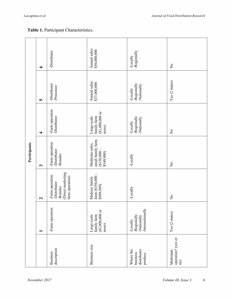
Data Analysis Interviews were transcribed verbatim and proofread for accuracy. Data were organized using a general inductive approach based on the grounded theory method, which has been previously published in similar qualitative research (Thomas, 2006; Freedman, 2009). This inductive approach allows insights to emerge directly from the data as opposed to confirming or denying previously defined hypotheses (Glaser and Strauss, 1967). Data coding was an iterative and collaborative process. Two researchers independently coded six pages of the interview transcripts, each developing a codebook that comprised the code name, abbreviation, definition/explanation, and examples. Researchers then met to compare their coding schemes, discussing agreements and discrepancies of assigned codes to ultimately merge their codebooks. This process was repeated two more times with four new pages of transcripts compared at each meeting. A crude assessment of inter-rater reliability was determined by calculating percentage agreement of the most frequently coded sections. A coding was considered an agreement if both researchers assigned the main idea of a text segment to the same code (Burla et al., 2008). Overall, inter-coder reliability of the transcripts was 90.9%. After establishing reliability, the remaining transcripts were organized using the qualitative data analysis software NVIVO. Similar to the initial coding process, a thematic content analysis was conducted from actual phrases used in the text to identify emerging ideas, patterns, and themes from the dataset based on volume of codes (Glaser and Strauss, 1967). Subtopics were identified for certain categories, and appropriate quotes that conveyed fundamental themes were noted (Thomas, 2006). The process resulted in categories that represented the most important themes from the data. Results Sample Demographics Table 1 displays data from the brief demographics survey, revealing characteristics of the six supply chain representatives who participated in the study. While two participants described their businesses as only one type within the produce supply chain (such as farm operation or distributor), the other four participants selected multiple descriptors. Results from this sample indicate there is not necessarily a clear distinction between supply chain entities. Participants included small, midsize, and large-scale family farms with distribution ranging from local to international. However, all participants described Phoenix-area markets as their primary distribution focus. The small and midsize family farms conducted their own distribution and delivery to outlets such as farmers’ markets, farm stands, community supported agriculture programs, and independent restaurants. The two large-scale family farms hired less-than-truckload shipping, distributed directly, or allowed customers to pick up product from their docks. Primary customers included retail chain supermarkets, small-format grocery stores, and downtown produce brokers or wholesalers who then disseminated some of that product to food service and smaller retailers. One of these participants also sold slightly older produce that would not meet chain store
Lacagnina et al. Journal of Food Distribution Research
November 2017 Volume 48, Issue 3
6
Table 1. Participant Characteristics.
Part
icip
ants
6 -Dis
tribu
tor
Ann
ual s
ales
: $5
0,00
0,00
0
-Loc
ally
-R
egio
nally
No
5 -Dis
tribu
tor
-Pro
cess
or
Ann
ual s
ales
: $3
7,00
0,00
0
-Loc
ally
-R
egio
nally
-N
atio
nally
Yes
(2 st
ates
)
4 -Far
m o
pera
tion
-Dis
tribu
tor
Larg
e-sc
ale
fam
ily fa
rm
($1,
000,
000
or
mor
e)
-Loc
ally
-R
egio
nally
-N
atio
nally
No
3 -Far
m o
pera
tion
-Dis
tribu
tor
-Ret
aile
r
Mod
erat
e-sa
les,
smal
l fam
ily fa
rm
($15
0,00
0 -
$349
,000
)
-Loc
ally
No
2 -Far
m o
pera
tion
-Dis
tribu
tor
-Ret
aile
r (D
irect
mar
ketin
g fa
rm o
pera
tion)
Mid
size
fam
ily
farm
($35
0,00
0 -
$999
,999
)
-Loc
ally
No
1 -Far
m o
pera
tion
Larg
e-sc
ale
fam
ily fa
rm
($1,
000,
000
or
mor
e)
-Loc
ally
-R
egio
nally
-N
atio
nally
-I
nter
natio
nally
Yes
(2 st
ates
)
Bus
ines
s de
scrip
tion
Bus
ines
s siz
e
Whe
re th
e bu
sine
ss
dist
ribut
es
prod
uce
Mul
tista
te
oper
atio
n? (y
es o
r no
)
Lacagnina et al. Journal of Food Distribution Research
November 2017 Volume 48, Issue 3
7
standards to secondary markets in Phoenix and Los Angeles. The distributor/processor delivered product to grocery stores, warehouse clubs, and other major distributors. The customer base of the final distributor included Phoenix-area schools, restaurants, “mom and pop” stores, and other retail markets. In the sections following, direct quotes from participants are followed by fabricated initials to ensure anonymity. Barriers Transportation costs Transportation costs were brought up by nearly all of the participants when asked about produce distribution challenges (noted by 5/6 participants; 28 references total). Several participants specifically mentioned logistical costs as a barrier to servicing smaller retailers or secondary outlets. Respondents noted the cost of the truck, the driver, insurance, fuel, maintenance, and minimum delivery costs as current and potential barriers.
“If it’s trying to schedule freight and trucks and all of that, in the end it almost becomes more trouble than it’s worth from a business sense.” [L.T.] “What are the challenges…um fuel costs, um, expensive delivery equipment, you know, do you need refrigerated trucks and that sort of thing. We don’t have that now but those would be helpful.” [D.R.]
Production Costs Local growers felt that staying in business and thriving as a farm was itself a challenge and described how the costs involved impacted their practices, pricing, and with whom they conducted business (5/6; 18 references). Production costs mentioned included field, labor, and storage prices. These production costs varied in relation to market variability. One grower explained that if a particular item saturated the market, the production costs associated with harvest and storage were often greater than revenue from sales. Hence, several growers opted to leave produce in the field (food waste) or donate produce to charity to minimize production costs and loss of revenue. Several growers described having limited profit margins within the produce supply chain as a result.
“Sometimes it’s actually more expensive for us to sell it than it is for us to just leave it in the field or donate it…It becomes harder and harder to be a farmer because it’s really cost prohibitive.” [L.T.]
Lack of Control Participants described several variables in the produce industry beyond their power of influence, including produce distribution challenges (4/6; 22 references). Respondents expressed this theme in relation to shorter shelf life, variation in produce appearance, weather fluctuations, a variable produce market, and retail stores accepting product. Participants specifically emphasized the diminishing quality of a perishable product and the resulting limits on where produce can be
Lacagnina et al. Journal of Food Distribution Research
November 2017 Volume 48, Issue 3
8
distributed depending on storage space, transportation, and retail standards. Several participants also mentioned how weather impacted growing capabilities and subsequent pricing. Especially on a small scale, production and volume vary to a greater extent than larger-scale production; as such, growers described a limitation on meeting demand for a larger volume of single items because they could not guarantee that level of production, nor did they generally have the capacity to store larger volumes and distribute it efficiently. This issue has been noted in previous work as well (Bloom and Hinrichs, 2011).
“The thing with produce is it’s not widgets. It’s different every day. The product you get in is different every day. Um, one day it could be perfect and the next day you could have bug damage. Um, some vegetables hold up better than others, you know, there’s all kinds of moving parts that affect what you do that you have zero control over…As a farmer you have no control over the weather, you have no control over the market, and you have no control over what the chain stores are gonna buy from you.” [L.T.]
Purchasing Power of the End Customer Participants identified retail customers’ purchasing power as a potential barrier to distributing to underserved areas in the Phoenix Valley (4/6; 15 references). One respondent noted that distribution depends on potential customers’ ability to buy enough product to make it worthwhile for the distributor to stop at the retail location. Several participants mentioned that they preferred to work with large-volume customers, and one participant expressed that their minimum order requirements and inability to break cases made them inaccessible to small food retailers. These findings mirror challenges identified in a previous report about providing fresh produce to small food stores (Laurison, 2014).
“I mean, it would behoove us to work with someone who orders a lot of volume because margins are so low, it is, there are volume items and you do better with volume. But even more than that it’s just the logistics of, ‘hey, we can only sell you two dozen of this, and if you can’t take two dozen, it’s zero or two dozen.’ We have no means to break it up.” [L.T.] “…if they don’t purchase at least 250 dollars’ worth of product, it becomes a loss to us.” [S.J.]
Financial Security Financial security emerged as a subtheme of end customers’ purchasing power (2/6; 7 references). This code represented statements several participants made about preferring to work with customers who provide financial security when it comes to getting paid for their product. One participant also commented that they only worked with business partners who have certain ratings in the “blue book,” which she described as an encyclopedia of company information and business statistics for all areas of farming business, including pay trends, trade practices, and credit scores. This allowed their business to minimize the potential of “getting burned” financially from not being paid for the perishable product they provide.
Lacagnina et al. Journal of Food Distribution Research
November 2017 Volume 48, Issue 3
9
“…with perishable product it’s not like you can take it back. And if that company can’t pay, you have the potential to take a huge loss and possibly never recoup expenses.” [L.T.] “When we’re looking for new business we’re generally looking for really steady opportunities, um, so we’re not necessarily looking for every individual small store.” [L.T.]
Affordability of Produce When asked about potential barriers to selling in underserved areas of Phoenix, five participants brought up the price point of produce (5/6; 11 references). This subtheme emerged as a barrier for both retail stores and customers purchasing fruits and vegetables. Some participants expressed that fresh produce tends to carry a higher price than energy-dense, low-nutrient foods such as potato chips. Several respondents specifically said that their produce prices were higher than processed foods derived from subsidized commodities such as wheat, corn, rice, and soybeans. In addition, small and midsize growers described having a higher pricing structure for their produce because of their smaller size, greater labor inputs, and higher land prices, potentially making them unaffordable for sale in low-income areas.
“What I know of, you know, trouble with the low-income food problems, has to do with limited resources for buying food, so buying the cheapest calories possible…I think it’s gonna take a shift in how we think of food and the value of food and value associated with the cost of food, when you can get a lot more Doritos, you know, for your money than fresh produce…” [D.R.] “…a lot of those places won’t purchase from us, because they can’t afford to purchase that. They need something much more reasonable to give to that customer.” [S.J.]
Strategies Alternative Distribution Channels Alternative distribution channels were identified as important strategies for increasing fresh fruit and vegetable access in low-income Phoenix neighborhoods (5/6; 18 references). Several participants identified the help of a third-party program such as a food hub or non-profit organization to assist with distribution and logistics. Two participants suggested the establishment of mobile markets that carry fresh, affordable produce to food desert neighborhoods. One distributor proposed redirecting food that is safe but would otherwise be wasted to be sold in these areas.
“If there was a non-profit involved that helped facilitate, you know, transporting produce to these areas. Or, um, partnered stores with farms, you know, then yeah, absolutely, but I think it would take something like a third-party to kind of facilitate that…” [L.T.]

Lacagnina et al. Journal of Food Distribution Research
November 2017 Volume 48, Issue 3
10
“…we really need to pull back in and look at some of these smaller format distribution models like food hubs.” [A.H.]
Incentive/Profit Participants identified the need for tax or economic incentives that would lessen the financial risk involved with distributing to low-volume stores (4/6; 14 references). Several participants noted that they would be interested in distributing to small food retailers in food deserts if there were funding to provide them with more efficient storage or transportation equipment, a tax incentive, or a “break-even” opportunity. These types of incentives have been identified in previous studies as important strategies for addressing barriers such as minimum order requirements and delivery fees from the retail perspective but not from perspectives further upstream in the supply chain. For example, many healthy corner store programs across the country offer store owners small stipends to reduce the risk associated with stocking new products such as fresh fruits and vegetables (Laurison, 2014; U.S. Department of Agriculture, 2016).
“…as a company too, you’re out there to be profitable. Um, so if there’s a break even, even to do something like that, that helps the community, then yeah, it’s something that we could do.” [S.J.]
Utilize Existing Infrastructure Two participants suggested utilizing and improving existing distribution systems and retail infrastructure as a strategy for increasing access to fresh, affordable food in low-income neighborhoods (2/6; 6 references). One participant suggested working with existing small food retailers in food desert areas to increase the availability of healthy items, a common public health approach for improving healthy food access (U.S. Department of Agriculture, 2016). Another participant suggested finding out who is already distributing to these areas and whether they would be interested in supplying produce to existing stores to maximize delivery efficiency. Other reports have explored more nuanced strategies for improving existing distribution systems to better serve small food retailers, such as establishing cooperative purchasing agreements among multiple small stores in a community and working with larger institutions such as hospitals and schools to add onto existing fresh produce orders (Laurison, 2014).
“From a distribution standpoint, I’d have to look at the model and see where those deserts are in conjunction with our customer base, and find out who would be willing to look into this as an opportunity to sell more product.” [P.L.] “…you know corner store and convenience stores, the ‘C’ store concepts. I think that’s a great idea because you’re using an existing system and you’re just changing it.” [A.H.]
Additional Insights Food Safety Regulations
Lacagnina et al. Journal of Food Distribution Research
November 2017 Volume 48, Issue 3
11
Many participants discussed food safety regulations, the costs associated with enforcing such regulations, and their impact on business partnerships (4/6; 22 references). While participants acknowledged the importance of food safety, several growers emphasized concerns over the added expense of implementing food safety programs and third-party audits such as Hazard Analysis and Critical Control Points (HACCP), Good Handling Practices (GHP), and Good Agricultural Practices (GAP) (Martinez, 2016). These certifications improve market access opportunities for growers as many distributors, retailers, and foodservice buyers require them as a condition of purchase. However, the documentation and infrastructure required for these certifications can be cost-prohibitive for small produce growers, preventing them from entering new markets. One large-scale grower felt that farmers were most impacted by potential financial implications of food safety issues. This caused them to work with vendors or distributors that could ensure safe transport and storage of their product. Two distributors expressed the need for total accountability from the growers they do business with and acknowledged that this prevented them from working with some small-scale local farmers.
“…it increases costs by a lot and it increases wariness from a farmer to, you know, even grow certain things or work with certain things because of concern.” [L.T.] “Unless the local farmers can, can get us a third-party audit certificate and show that they’re HACCP certified, uh, we stay away from that.” [S.J.]
Donations Nearly all respondents donate excess produce to a network of food banks and saw this as an effective strategy to get produce into low-income areas (5/6; 17 references). Two respondents explained that excess product is typically a result of produce appearance not meeting chain store specifications or greater than expected yields.
“We have always focused on getting our produce into low-income areas by donating and participating in the Statewide Gleaning project…Our gleaning program has allowed us to donate 1.5 – 2 million pounds of produce annually to food banks to distribute out and get into the hands of people who need access to fresh produce.” [A.H.] “If I don’t know where to go with it, it goes to the food bank.” [P.L.]
Discussion To date, little research exists focusing on potential barriers and strategies of the supply chain in relation to food deserts. This study provided novel insight into this important aspect of the issue. In particular, the relations between supply chain entities represented a variety of potential barriers that could contribute to the perpetual lack of healthy, affordable fresh food in food desert areas. Participants perceived numerous obstacles in servicing Phoenix-area food deserts. Several local growers described the lack of control inherent in working with a perishable product, production costs, and market volatility as challenges to simply remaining financially sustainable as a farm.

Lacagnina et al. Journal of Food Distribution Research
November 2017 Volume 48, Issue 3
12
Participants also mentioned several distribution barriers: minimum delivery requirements greater than the needs of the typical small store, an inability to break up case sizes for low-volume orders, transportation costs, and the higher price point of their produce relative to other food options. In addition, many participants expressed how new food safety regulations introduce added costs and uncertainties within farmer-distributor-retailer business partnerships. These results reflect those from similar work conducted by the Food Trust among small store operators (Bentzel et al., 2015). Participants also suggested multiple strategies for overcoming these barriers and other related issues. As financial viability was a common concern among participants, they commonly suggested the need for financial incentives or a “good break-even” to interest them in new business in these areas. Participants also discussed alternative distribution/retail channels such as mobile markets and food hubs as potential strategies for alleviating logistical and transportation costs and improving healthy food accessibility for residents of low-income, low-access areas, among other benefits. As an additional insight, nearly all participants described currently donating excess produce to local food banks as their primary means of distributing fresh fruits and vegetables to low-income communities. These insights may be useful to practitioners and advocates interested in exploring systems solutions to the problem of healthy food access. Examples exist around the United States of local foods initiatives that simultaneously target the dual goals of improved food security and community development (Phillips and Wharton, 2015). Programs include successful food hubs, processing centers, and other novel models of fresh food aggregation and delivery. Further, researchers have explored innovations in local food social entrepreneurship that provide insights into how best to plan the implementation of these types of programs and organizations (Horst et al., 2011). While greater insight and understanding of the issues in the fresh produce supply chain was obtained, this study does have some limitations that provide opportunities for future research. Due to the qualitative, exploratory nature of the study, the results reveal thematic findings but do not intend to offer conclusive answers to the research questions. Also, because of the recruitment methodology and small sample size, the sample is not representative of the larger population. Instead, these findings provide insights into one supply chain stream in order to identify emergent and critical issues that could be explored in future research regarding how pervasive, or generalized, they might be. As such, next steps would be to follow up with a survey informed by these results, in which data obtained could be quantified and extrapolated to a larger population. Conclusion This research provides important insights into the challenges faced by fresh produce supply chain members in servicing food desert areas. Findings from this qualitative, exploratory study also shed light on potential strategies for overcoming such barriers from the supply chain perspective. Although some of the findings are consistent with previous research, such as concerns about cost of operations and lack of control over multiple factors of small-farm operations, other insights have a degree of novelty as the grower and distributor perspective has not been fully represented in the literature. For example, concerns about food safety regulations
Lacagnina et al. Journal of Food Distribution Research
November 2017 Volume 48, Issue 3
13
represent an important concern, and novel opportunity for intervention, from the grower and distributor perspective. Similarly, interest among these groups in alternative distribution strategies, such as food hubs, suggests an openness to new ways of coordinating production to improve access. These data serve to guide further research, which may ultimately better inform policies and programs addressing healthy food access and working toward a more equitable food system. Acknowledgments This study was supported by a USDA Higher Education Grant (#026885-001). The contents of this article are the responsibility of the authors and do not necessarily represent the views of the funding source. References Bentzel, D., S. Weiss, M. Bucknum, and K. Shore. 2015. Healthy Food and Small Stores:
Strategies to Close the Distribution Gap. Philadelphia, PA: The Food Trust.
Bloom, J.D., and C. Hinrichs. 2011. “Moving Local Food through Conventional Food System Infrastructure: Value Chain Framework Comparisons and Insights.” Renewable Agriculture and Food Systems 26(1):13–23.
Burla, L., B. Knierim, J. Barth, K. Liewald, M. Duetz, and T. Abel. 2008. “From Text to Codings: Intercoder Reliability Assessment in Qualitative Content Analysis.” Nursing Research 57(2):113–117.
Coleman-Jensen, A., C. Gregory, and A. Singh. 2014. Household Food Security in the United States in 2013. Washington, DC: U.S. Department of Agriculture, Eeconomic Research Service, Economic Research Report 173, September.
Chung, C., and S.L. Myers. 1999. “Do the Poor Pay More for Food? An Analysis of Grocery Store Availability and Food Price Disparities.” Journal of Consumer Affairs 33(2):276–296.
Drewnowski, A. 2009. “Obesity, Diets, and Social Inequalities.” Nutrition Reviews 67 (Suppl 1):S36–39.
Freedman, D.A. 2009. “Local Food Environments: They’re All Stocked Differently.” American Journal of Community Psychology 44(3–4):382–393.
Gittelsohn, J., M. Franceschini, I. Rasooly, A. Ries, L. Ho, W. Pavlovich, V. Santos, S. Jennings, and K. Frick. 2008. “Understanding the Food Environment in a Low-Income Urban Setting: Implications for Food Store Interventions.” Journal of Hunger & Environmental Nutrition 2(2–3):33–50.

Lacagnina et al. Journal of Food Distribution Research
November 2017 Volume 48, Issue 3
14
Glaser, B.G., and A.L. Strauss. 1967. Discovery of Grounded Theory: Strategies for Qualitative Research. Chicago: Aldine.
Hawkes, C. 2009. “Identifying Innovative Interventions to Promote Healthy Eating Using Consumption-Oriented Food Supply Chain Analysis.” Journal of Hunger & Environmental Nutrition 4(3–4):336–356.
Hendrickson, D., C. Smith, and N. Eikenberry. 2006. “Fruit and Vegetable Access in Four Low-Income Food Deserts Communities in Minnesota.” Agriculture and Human Values 23(3):371–383.
Hill, J. 1998. “Environmental Contributions to the Obesity Epidemic.” Science 280(5368):1371–1374.
Hilmers, A., D.C. Hilmers, and J. Dave. 2012. “Neighborhood Disparities in Access to Healthy Foods and their Effects on Environmental Justice.” American Journal of Public Health 102(9):1644–1654.
Horst, M., E. Ringstrom, S. Tyman, M. Ward, V. Werner, and B. Born. 2011. “Toward a More Expansive Understanding of Food Hubs.” Journal of Agriculture, Food Systems, and Community Development 2(1):209–225.
Larson, C., A. Haushalter, T. Buck, D. Campbell, T. Henderson, and D. Schlundt. 2013. “Development of a Community-Sensitive Strategy to Increase Availability of Fresh Fruits and Vegetables in Nashville’s Urban Food Deserts, 2010–2012.” Preventing Chronic Disease 10:E125.
Larson, N.I., M.T. Story, and M.C. Nelson. 2009. “Neighborhood Environments: Disparities in Access to Healthy Foods in the U.S.” American Journal of Preventive Medicine 36(1):74–81.
Laurison, H.B. 2014. Providing Fresh Produce in Small Food Stores. Oakland, CA: ChangeLab Solutions.
Martinez, S.W. 2016. “Policies Supporting Local Food in the United States.” Agriculture 6(3):43.
Morland, K., A.V. Diez Roux, and S. Wing. 2006. “Supermarkets, Other Food Stores, and Obesity.” American Journal of Preventive Medicine 30(4):333–339.
Odoms-Young, A.M., S.N. Zenk, A. Karpyn, G.X. Ayala, and J. Gittelsohn. 2012. “Obesity and the Food Environment Among Minority Groups.” Current Obesity Reports 1(3):141–151.
Patton, M.Q. 1990. Qualitative Evaluation and Research Methods, 2nd ed. Newbury Park, CA: Sage.

Lacagnina et al. Journal of Food Distribution Research
November 2017 Volume 48, Issue 3
15
Phillips, R., and C. Wharton. 2015. Local Food Systems and Community Well Being. New York: Taylor & Francis.
Strauss, A., and J. Corbin. 1990. Basics of Qualitative Research: Grounded Theory Procedures and Techniques. Newbury Park, CA: Sage.
Thomas, D.R. 2006. “A General Inductive Approach for Analyzing Qualitative Evaluation Data.” American Journal of Evaluation 27(2):237–246.
U.S. Census Bureau. 2015. Arizona: US Census Bureau State City QuickFacts. Washington DC, April.
U.S. Department of Agriculture. 2016. Healthy Corner Stores: Making Corner Stores Healthier Places to Shop. Washington, DC: U.S. Department of Agriculture, Food and Nutrition Service, Report FNS-621, June.
U.S. Department of Agriculture. 2017. Food Access Research Atlas. Washington, DC: U.S. Department of Agriculture, Economic Research Service. Available online: https://www.ers.usda.gov/data-products/food-access-research-atlas/
Wolfersteig, W.L., H. Lewis, T. Musgrave, T. Johnson, T. Wolven, and F.F. Marsiglia. 2011. 2010 Arizona Health Survey: Food, Housing Insecurity and Health. Phoenix: Arizona Health Survey, November.
Journal of Food Distribution Research Volume 48, Issue 3
November 2017 Volume 48, Issue 3
16
Impacts of Food Safety Recalls and
Consumer Information on Restaurant Performance
J. Ross Pruitta! and Rodney B. Holcomb
aAssociate Professor, Department of Agriculture Geosciences, and Natural Resources,
University of Tennessee at Martin, 206 Brehm Hall Martin, TN, 38238 USA
bProfessor, Department of Agricultural Economics
Oklahoma State University, 114 Food & Agricultural Products Center, Stillwater, OK, 74078 USA
Abstract
Consumer expenditures on purchases of food away from home have risen in recent years to comprise nearly half of consumer food budgets. Using the monthly National Restaurant Association Restaurant Performance Index, we seek to determine the factors influencing restaurateurs’ perceptions of their current situation, same-store sales, and customer traffic from July 2002 through March 2017. Macroeconomic variables have little impact on restaurant performance, but concerns about public health perceptions do impact restaurateurs’ outlook. Concerns over the link between meat and poultry consumption and cancer also negatively impact restaurant owners’ perceptions of performance. Keywords: food away from home, food safety, health, nutrition, restaurant performance
!Corresponding author: Tel: (731) 881-7254
Email: [email protected]
Pruitt and Holcomb Journal of Food Distribution Research
November 2017 Volume 48, Issue 3
17
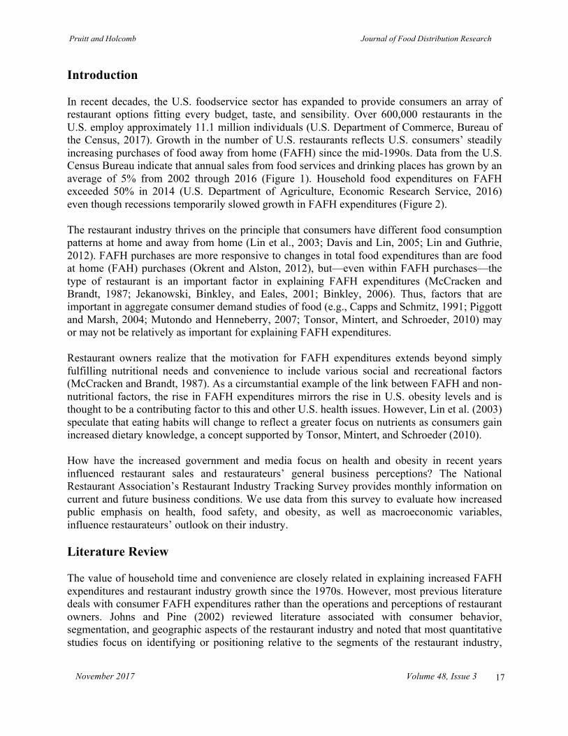
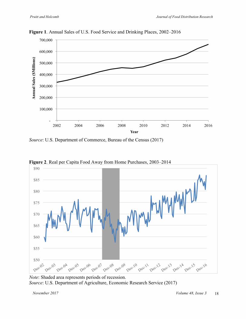
Introduction In recent decades, the U.S. foodservice sector has expanded to provide consumers an array of restaurant options fitting every budget, taste, and sensibility. Over 600,000 restaurants in the U.S. employ approximately 11.1 million individuals (U.S. Department of Commerce, Bureau of the Census, 2017). Growth in the number of U.S. restaurants reflects U.S. consumers’ steadily increasing purchases of food away from home (FAFH) since the mid-1990s. Data from the U.S. Census Bureau indicate that annual sales from food services and drinking places has grown by an average of 5% from 2002 through 2016 (Figure 1). Household food expenditures on FAFH exceeded 50% in 2014 (U.S. Department of Agriculture, Economic Research Service, 2016) even though recessions temporarily slowed growth in FAFH expenditures (Figure 2). The restaurant industry thrives on the principle that consumers have different food consumption patterns at home and away from home (Lin et al., 2003; Davis and Lin, 2005; Lin and Guthrie, 2012). FAFH purchases are more responsive to changes in total food expenditures than are food at home (FAH) purchases (Okrent and Alston, 2012), but—even within FAFH purchases—the type of restaurant is an important factor in explaining FAFH expenditures (McCracken and Brandt, 1987; Jekanowski, Binkley, and Eales, 2001; Binkley, 2006). Thus, factors that are important in aggregate consumer demand studies of food (e.g., Capps and Schmitz, 1991; Piggott and Marsh, 2004; Mutondo and Henneberry, 2007; Tonsor, Mintert, and Schroeder, 2010) may or may not be relatively as important for explaining FAFH expenditures. Restaurant owners realize that the motivation for FAFH expenditures extends beyond simply fulfilling nutritional needs and convenience to include various social and recreational factors (McCracken and Brandt, 1987). As a circumstantial example of the link between FAFH and non-nutritional factors, the rise in FAFH expenditures mirrors the rise in U.S. obesity levels and is thought to be a contributing factor to this and other U.S. health issues. However, Lin et al. (2003) speculate that eating habits will change to reflect a greater focus on nutrients as consumers gain increased dietary knowledge, a concept supported by Tonsor, Mintert, and Schroeder (2010). How have the increased government and media focus on health and obesity in recent years influenced restaurant sales and restaurateurs’ general business perceptions? The National Restaurant Association’s Restaurant Industry Tracking Survey provides monthly information on current and future business conditions. We use data from this survey to evaluate how increased public emphasis on health, food safety, and obesity, as well as macroeconomic variables, influence restaurateurs’ outlook on their industry. Literature Review The value of household time and convenience are closely related in explaining increased FAFH expenditures and restaurant industry growth since the 1970s. However, most previous literature deals with consumer FAFH expenditures rather than the operations and perceptions of restaurant owners. Johns and Pine (2002) reviewed literature associated with consumer behavior, segmentation, and geographic aspects of the restaurant industry and noted that most quantitative studies focus on identifying or positioning relative to the segments of the restaurant industry,
Pruitt and Holcomb Journal of Food Distribution Research
November 2017 Volume 48, Issue 3
18
Figure 1. Annual Sales of U.S. Food Service and Drinking Places, 2002–2016
Source: U.S. Department of Commerce, Bureau of the Census (2017) Figure 2. Real per Capita Food Away from Home Purchases, 2003–2014
Note: Shaded area represents periods of recession. Source: U.S. Department of Agriculture, Economic Research Service (2017)
-
100,000
200,000
300,000
400,000
500,000
600,000
700,000
2002 2004 2006 2008 2010 2012 2014 2016
Ann
ual S
ales
($M
illio
ns)
Year
$50
$55
$60
$65
$70
$75
$80
$85
$90

Pruitt and Holcomb Journal of Food Distribution Research
November 2017 Volume 48, Issue 3
19
reflecting restaurant heterogeneity. Binkley and Bales (1998) stated that availability and population density tend to be more important than demographic factors in determining fast food expenditures. With FAFH expenditures exceeding those for FAH for the first time in 2014 (U.S. Department of Agriculture, Economic Research Service, 2016), studies of consumers’ valuations for convenience and household time have been the primary sources of information on FAFH expenditures and their impacts on the restaurant industry. Jekanowski, Binkley, and Eales (2001) suggested that growth in FAFH expenditures is tied to an increasing supply of restaurants (i.e., availability and options), which decreases the effective cost of the food (i.e., distance traveled plus food cost). This results in what they call an “increasing supply of convenience,” especially for quick-service restaurants, rather than a change in consumer tastes and preferences that would result in increased demand for FAFH expenditures. Research by Binkley and Bales (1998) and Binkley (2006) supports the importance of convenience from a location and time perspective in explaining the increase in FAFH expenditures. This increased supply of convenience corresponds to a period in which women have increasingly become part of the U.S. labor force. Female participation in the labor force approached 60% for most of the first decade of the 2000s but declined slightly during the Great Recession. Although women are less likely to dine out (Binkley, 2006), their labor force participation rate has been used to explain shifts in consumer demand for FAFH and meat products in general (Yen, 1993; Tonsor, Mintert, and Schroeder, 2010). Other factors impacting FAFH demand are general economic conditions, consumer demographics, nutritional knowledge, and eating habits. Lee and Ha (2012) found positive correlations between restaurant industry activity and GDP yet noted that relatively few studies have directly investigated the impacts of economic recessions or key economic indicators on the restaurant industry. Hua, Xiao, and Yost (2013) further noted that the industry “exhibits strong seasonality and cyclical patterns,” meaning that restaurant owners must recognize and develop strategies for various seasons and cycles. Nayga and Capps (1992), Jekanowski, Binkley, and Eales (2001), and Binkley (2006) accounted for income but ignored the impact of economic recessions on demand for FAFH. The diversity in demand for FAFH, and the restaurant options catering to those demands, creates challenges for assessing the impacts of economic conditions on the restaurant industry as a whole (Lee and Ha, 2012; Wang, 2012; Hua, Ziao, and Yost, 2013; Liu, Kasteridis, and Yen, 2013). Concerns about increasing levels of U.S. consumer obesity have often been a motivating factor for “eating out” studies, due to concerns about the nutritional quality of FAFH (Lin and Frazao, 1997; Jekanowski, Binkley, and Eales, 2001; Young and Nestle, 2002). During the period of 2005–2008, nearly one-third of calories consumed in the United States came from FAFH sources (Lin and Guthrie, 2012). Anderson and Matsa (2011) found that consumers adjust their caloric intake following consumption of FAFH, which is consistent with Binkley (2006) and Yen, Lin, and Davis (2008), who stated that greater nutritional knowledge can impact food choices from FAFH sources.
Pruitt and Holcomb Journal of Food Distribution Research
November 2017 Volume 48, Issue 3
20
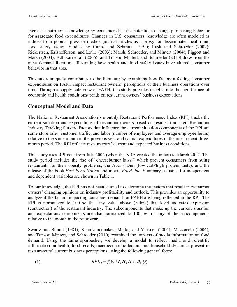
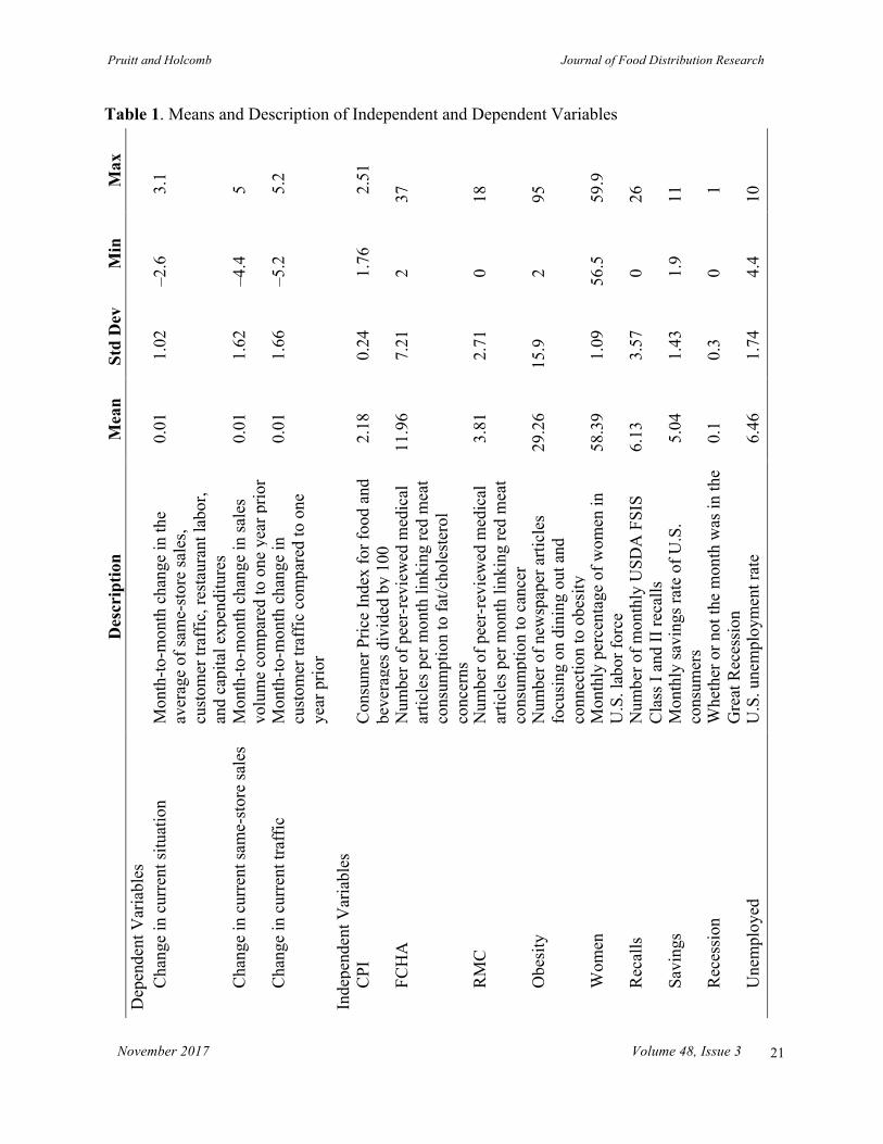
Increased nutritional knowledge by consumers has the potential to change purchasing behavior for aggregate food expenditures. Changes in U.S. consumers’ knowledge are often modeled as indices from popular press or medical journal articles as a proxy for disseminated health and food safety issues. Studies by Capps and Schmitz (1991); Lusk and Schroeder (2002); Rickertsen, Kristofferson, and Lothe (2003); Marsh, Schroeder, and Mintert (2004); Piggott and Marsh (2004); Adhikari et al. (2006); and Tonsor, Mintert, and Schroeder (2010) draw from the meat demand literature, illustrating how health and food safety issues have altered consumer behavior in that area. This study uniquely contributes to the literature by examining how factors affecting consumer expenditures on FAFH impact restaurant owners’ perceptions of their business operations over time. Through a supply-side view of FAFH, this study provides insights into the significance of economic and health conditions/trends on restaurant owners’ business expectations. Conceptual Model and Data The National Restaurant Association’s monthly Restaurant Performance Index (RPI) tracks the current situation and expectations of restaurant owners based on results from their Restaurant Industry Tracking Survey. Factors that influence the current situation components of the RPI are same-store sales, customer traffic, and labor (number of employees and average employee hours) relative to the same month in the previous year and capital expenditures in the most recent three-month period. The RPI reflects restaurateurs’ current and expected business conditions. This study uses RPI data from July 2002 (when the NRA created the index) to March 2017. The study period includes the rise of “cheeseburger laws,” which prevent consumers from suing restaurants for their obesity problems; the Atkins Diet (low-carb/high protein diets); and the release of the book Fast Food Nation and movie Food, Inc. Summary statistics for independent and dependent variables are shown in Table 1. To our knowledge, the RPI has not been studied to determine the factors that result in restaurant owners’ changing opinions on industry profitability and outlook. This provides an opportunity to analyze if the factors impacting consumer demand for FAFH are being reflected in the RPI. The RPI is normalized to 100 so that any value above (below) that level indicates expansion (contraction) of the restaurant industry. The subcomponents that make up the current situation and expectations components are also normalized to 100, with many of the subcomponents relative to the month in the prior year. Swartz and Strand (1981); Kalaitzandonakes, Marks, and Vickner (2004); Mazzocchi (2006); and Tonsor, Mintert, and Schroeder (2010) examined the impacts of media information on food demand. Using the same approaches, we develop a model to reflect media and scientific information on health, food recalls, macroeconomic factors, and household dynamics present in restaurateurs’ current business perceptions, using the following general form:
(1) RPIt-1 = f(V, M, H, HA, R, Q)
Pruitt and Holcomb Journal of Food Distribution Research
November 2017 Volume 48, Issue 3
21
Table 1. Means and Description of Independent and Dependent Variables M
ax
3.1
5
5.2
2
.51
37
18
95
59.9
26
11
1
10
Min
–2
.6
–4.4
–5.2
1
.76
2
0
2
56.5
0
1.9
0
4.4
Std
Dev
1
.02
1.6
2
1.6
6 0
.24
7.2
1
2.7
1
15.9
1.0
9
3.5
7
1.4
3
0.3
1.7
4
Mea
n 0
.01
0.0
1
0.0
1 2
.18
11.9
6
3.8
1
29.2
6
58.3
9
6.13
5.0
4
0.1
6.4
6
Des
crip
tion
Mon
th-to
-mon
th c
hang
e in
the
aver
age
of sa
me-
stor
e sa
les,
cust
omer
traf
fic, r
esta
uran
t lab
or,
and
capi
tal e
xpen
ditu
res
Mon
th-to
-mon
th c
hang
e in
sale
s vo
lum
e co
mpa
red
to o
ne y
ear p
rior
Mon
th-to
-mon
th c
hang
e in
cu
stom
er tr
affic
com
pare
d to
one
ye
ar p
rior
Con
sum
er P
rice
Inde
x fo
r foo
d an
d be
vera
ges d
ivid
ed b
y 10
0 N
umbe
r of p
eer-
revi
ewed
med
ical
ar
ticle
s per
mon
th li
nkin
g re
d m
eat
cons
umpt
ion
to fa
t/cho
lest
erol
co
ncer
ns
Num
ber o
f pee
r-re
view
ed m
edic
al
artic
les p
er m
onth
link
ing
red
mea
t co
nsum
ptio
n to
can
cer
Num
ber o
f new
spap
er a
rticl
es
focu
sing
on
dini
ng o
ut a
nd
conn
ectio
n to
obe
sity
M
onth
ly p
erce
ntag
e of
wom
en in
U
.S. l
abor
forc
e N
umbe
r of m
onth
ly U
SDA
FSI
S C
lass
I an
d II
reca
lls
Mon
thly
savi
ngs r
ate
of U
.S.
cons
umer
s W
heth
er o
r not
the
mon
th w
as in
the
Gre
at R
eces
sion
U
.S. u
nem
ploy
men
t rat
e
Dep
ende
nt V
aria
bles
Cha
nge
in c
urre
nt si
tuat
ion
C
hang
e in
cur
rent
sam
e-st
ore
sale
s
C
hang
e in
cur
rent
traf
fic
Inde
pend
ent V
aria
bles
CPI
F
CH
A
R
MC
O
besi
ty
W
omen
R
ecal
ls
S
avin
gs
R
eces
sion
U
nem
ploy
ed
Pruitt and Holcomb Journal of Food Distribution Research
November 2017 Volume 48, Issue 3
22
where RPIt-1 is the change in the RPI subcomponent in month t from the previous month, V denotes the convenience and value of household time, M is a vector of macroeconomic variables, H is a vector containing health research information, HA is an index of media stories on restaurants, and R is the number of monthly Class I and II recalls issued by the U.S. Department of Agriculture’s Food Safety and Inspection Service (USDA FSIS). Quarterly dummy variables, denoted as Q, are also included for the first, second, and third quarters to account for seasonality in estimated models. For this study, the V vector is the percentage of women in the U.S. labor force from the Bureau of Labor Statistics. Inclusion of this variable is consistent with previous literature as a proxy for the value of household time. Included macroeconomic variables in M are the monthly per capita savings rate from the Bureau of Economic Analysis, the Consumer Price Index for food and beverages,1 the unemployment rate from the Bureau of Labor Statistics, and whether the month was part of a recession according to the National Bureau of Economic Research. These independent macroeconomic variables are consistent with previous literature explaining FAFH purchases. We also include the lagged unemployment rate to capture any lingering effects on restaurateurs’ perceptions of current business outlook based on a period greater than the current and previous monthly employment rates. We seek to examine how factors shown to impact overall food demand impact restaurant owners’ perceptions of current restaurant sales and customer traffic, as measured by the RPI’s subcomponents. Using Class I or Class II recalls from USDA FSIS is consistent with previous literature (Marsh, Schroeder, and Mintert, 2004; Tonsor, Mintert, and Schroeder, 2010), although previous studies segregated recalls by meat type (beef, pork, poultry), whereas we use an aggregate recall number. These two classes of recalls are used due to the possibility these events may result in a health hazard to consumers. The number of recalls occurring in a month may also undermine consumer confidence in the U.S. food supply and directly impact restaurant performance. We considered including recalls from the Food and Drug Administration (FDA) but ultimately decided against it because of the large number of recalls associated with mislabeling and undeclared allergens. FDA recalls also tend to involve a greater number of smaller suppliers and smaller geographic areas of impact relative to the broad-reaching impacts of large-volume recalls in the highly concentrated meat and poultry sector. We created three indices: two in the H vector and one in the HA vector. The two indices in the H vector were a fat, cholesterol, heart disease, and arteriosclerosis (FCHA) index and an index measuring the connection of red meat and poultry consumption with cancer. Each of these two indices was created using a monthly count of the number of articles returned in the Medline database for English-language journals. The FCHA index replicates the previous efforts of Rickertsen, Kristofferson, and Lothe (2003) and Tonsor, Mintert, and Schroeder (2010). To coincide with the RPI, our FCHA index is a monthly article count for ‘{(fat or cholesterol) AND (heart disease or arteriosclerosis) AND (diet)}’. The second index in the H vector was a monthly count of articles in the Medline database of English-language medical journals for the connection between red meat and poultry consumption and cancer (RMC). Search terms used for this RMC variable were ‘{(red meat or poultry) AND (diet) AND (cancer)}’. 1 We thank a reviewer for this suggestion.

Pruitt and Holcomb Journal of Food Distribution Research
November 2017 Volume 48, Issue 3
23
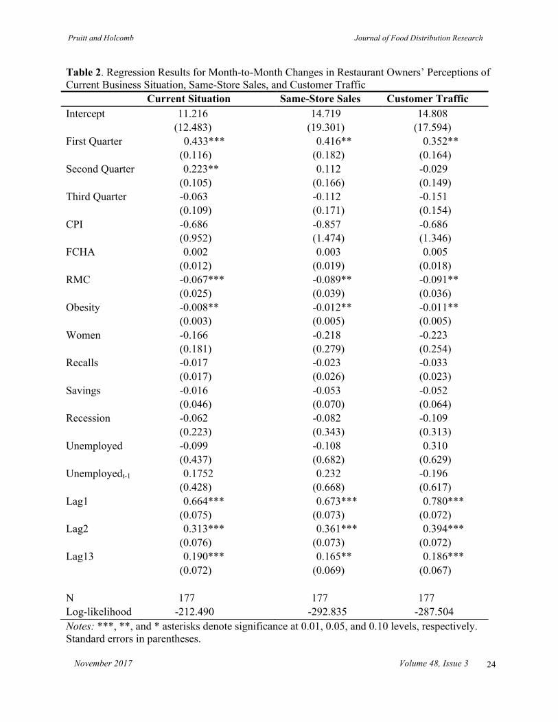
The third index reflects the increased prevalence and concern about obesity levels in the United States, as indicated by monthly U.S. newspaper articles on these topics for the HA vector. Using the Lexis-Nexis database, we searched for ‘{(restaurant or fast food or dining out) AND (obesity) AND NOT (editorial)}’ to determine the total number of articles expressing concern about restaurants and their contribution to obesity. We include the ‘AND NOT (editorial)’ to exclude editorials and letters to the editor, following pre-testing of this search term. Reviews of restaurants and books were also excluded from our final count. Duplicate articles were also removed from the final monthly count. We did not address the monthly change in the RPI value, as the aggregate RPI value is a simple average of the current and expectations components. Furthermore, we do not discuss models for the aggregate expectations index component or the subcomponents of the expectations index due to a lack of significance among independent variables aside from the quarterly dummy variables. The fact that several of the expectations subcomponents are for six months in the future, relative to that month one year prior, may be contribute to a lack of significance among explanatory variables. Additionally, restaurateurs’ future expectations may be based more on hope than true expectations of future business conditions. Results Initial models were estimated in ordinary least squares, but autocorrelation was detected. Subsequent estimations employed maximum likelihood in the PROC AUTOREG module of SAS 9.4. The appropriate number of autocorrelated errors was determined using the “backstep” feature in SAS as well as by testing for conditional heteroskedasticity. Results of the monthly change in the current situations model are shown in Table 2. There is evidence of some seasonal influences in restaurant owners’ business expectations, as the owners’ views of business conditions are statistically significantly higher in the first and second quarter of each year than in the fourth quarter. Including the CPI food and beverage variable resulted in the expected negative impact on restaurant performance, but it was insignificant. Increased medical article counts on the link between red meat and poultry consumption and cancer had a negative impact on the month-to-month change in the current situation of restaurant owners. The number of recalls also had a negative impact on the current restaurant situation, while the number of newspaper articles linking obesity concerns and restaurants also had a small but statistically significant negative impact on the current situation perceptions of owners. Same-Store Sales Volume The results for month-to-month change in same-store sales volume were similar to the results for month-to-month change in aggregate current situation. First quarter expectations for sales and customer traffic were also statistically significantly higher than fourth quarter RPI measures. This may be due to the prevalence of at-home holiday meals and expenditure shifts to holiday shopping that impacted FAFH expenditures and overall restaurant patronage of consumers in the fourth quarter.
Pruitt and Holcomb Journal of Food Distribution Research
November 2017 Volume 48, Issue 3
24
Table 2. Regression Results for Month-to-Month Changes in Restaurant Owners’ Perceptions of Current Business Situation, Same-Store Sales, and Customer Traffic Current Situation Same-Store Sales Customer Traffic Intercept 11.216 14.719 14.808 (12.483) (19.301) (17.594) First Quarter 0.433*** 0.416** 0.352** (0.116) (0.182) (0.164) Second Quarter 0.223** 0.112 -0.029 (0.105) (0.166) (0.149) Third Quarter -0.063 -0.112 -0.151 (0.109) (0.171) (0.154) CPI -0.686 -0.857 -0.686 (0.952) (1.474) (1.346) FCHA 0.002 0.003 0.005 (0.012) (0.019) (0.018) RMC -0.067*** -0.089** -0.091** (0.025) (0.039) (0.036) Obesity -0.008** -0.012** -0.011** (0.003) (0.005) (0.005) Women -0.166 -0.218 -0.223 (0.181) (0.279) (0.254) Recalls -0.017 -0.023 -0.033 (0.017) (0.026) (0.023) Savings -0.016 -0.053 -0.052 (0.046) (0.070) (0.064) Recession -0.062 -0.082 -0.109 (0.223) (0.343) (0.313) Unemployed -0.099 -0.108 0.310 (0.437) (0.682) (0.629) Unemployedt-1 0.1752 0.232 -0.196 (0.428) (0.668) (0.617) Lag1 0.664*** 0.673*** 0.780*** (0.075) (0.073) (0.072) Lag2 0.313*** 0.361*** 0.394*** (0.076) (0.073) (0.072) Lag13 0.190*** 0.165** 0.186*** (0.072) (0.069) (0.067) N 177 177 177 Log-likelihood -212.490 -292.835 -287.504 Notes: ***, **, and * asterisks denote significance at 0.01, 0.05, and 0.10 levels, respectively. Standard errors in parentheses.

Pruitt and Holcomb Journal of Food Distribution Research
November 2017 Volume 48, Issue 3
25
Medical articles linking red meat and poultry to cancer and the number of USDA FSIS recalls had a negative impact on month-to-month changes in same-store sales. The obesity index variable had a stronger, negative impact on sales volumes compared to the aggregate current situation variable. We cannot explain why the fat, cholesterol, and arteriosclerosis (FCHA) index had a small but positive impact on explaining changes in same-stores volume, although the parameter estimates were not statistically significant. Collectively, these findings are consistent with Binkley (2006) and Yen, Lin, and Davis (2008), who stated that greater nutritional knowledge can impact FAFH patterns of consumers. Monthly Customer Traffic As with changes in owners’ current situation assessments and same-store sales, seasonal differences were apparent in customer traffic. Similar to same-store sales, changes in monthly customer traffic were significantly higher during the first quarter than in the fourth quarter. As previously stated, this may be due to the propensity of fourth-quarter holiday meals at home impacting restaurant patronage. The change in monthly customer traffic was negatively impacted by the number of monthly medical articles linking red meat and poultry consumption with cancer. Newspaper articles mentioning the link between restaurants and obesity also exhibited a negative correlation with month-to-month changes in customer traffic. As with the change in the same-store sales dependent variable, the FCHA index exhibited a small but positive (and insignificant) influence on customer traffic. Overall Findings for Unemployment and Women in the Workforce Current unemployment, lagged unemployment, and the percentage of women in the workforce did not significantly impact changes in owners’ current situation perceptions, same-store sales, or customer traffic. Unemployment percentages may not have provided an accurate measure of overall workforce participation during the evaluation period, as the changes in active job seekers resulting from the Great Recession impacted the “true” unemployment measures. Increased female participation in the U.S. labor force had a negative impact on changes in owners’ current situations, same-store sales, and customer traffic. While the parameter estimates were not statistically significant, the negative sign on the coefficients contradicts previous studies. However, over the evaluation period the total magnitude change in female workforce participation was roughly 3%, even considering the impacts of the Great Recession. That lack of variation may suggest a longer-term sustained level of female workforce participation. With women less likely to dine out (Binkley, 2006), our findings suggest that restaurateurs are not being impacted in their current conditions, same-store sales, or customer traffic by the increased female labor-force participation rate. Stated differently, the female labor participation rate has reached a saturation point such that restaurateurs are not impacted by the small changes in the rate seen during our study period. Although recalls included in each of the three models were negative, none was significant. As Knight, Worosz, and Todd (2007) have stated, consumers feel that restaurants were “good” on
Pruitt and Holcomb Journal of Food Distribution Research
November 2017 Volume 48, Issue 3
26
their commitment to food safety. Furthermore, these authors found that commitment to food safety issues did not impact the frequency of eating at restaurants. This confirms our finding of insignificance of recalls impacting restaurateurs’ current conditions, same-store sales, and customer traffic. Similarly, Knight, Worosz, and Todd stated that respondents felt other parts of the supply chain (e.g., processors, manufacturers, and farmers) were more capable of ensuring food safety than restaurants. Conclusions Restaurants continue to be an integral part of U.S. consumers’ food consumption patterns due, in part, to the convenience and diversity of menu options offered. However, the factors that impact restaurant owners’ perceptions of industry performance are not well understood. This study sought to improve our understanding of the roles that health and nutrition information, food safety recalls, and general economic conditions play in restaurant owners’ perceptions of their industry. We find that the number of medical articles examining links between cancer and red meat and poultry consumption and newspaper articles linking restaurants to obesity have negative impacts on month-to-month current outlook, same-store sales, and customer traffic of U.S. restaurants, as measured by the National Restaurant Association’s Restaurant Performance Index. These factors were consistent in their magnitude, regardless of the dependent variable (current situation, same-store sales, or customer traffic). Because restaurants provide entertainment and ambiance in addition to fulfilling consumers’ nutritional needs, the impact of obesity warrants further research efforts. However, information on the number of restaurants included in the monthly RPI is necessary for such efforts. Although the models we estimated included a monthly count of obesity-related articles in U.S. newspapers, similar results were found when a three-month moving average of obesity-related articles was included in the models. There was some evidence of seasonality in restaurateurs’ responses on their current situation, as evidenced by visual analysis of the data in Figure 2. Somewhat surprisingly, most of the macroeconomic variables included were not significant in explaining the month-to-month change in restaurant outlook even during the downturn in FAFH purchases that occurred in the Great Recession. This may be a reflection of the dataset spanning fifteen years―a period over which there was significant growth in the restaurant industry (approximately 20% growth in the number of restaurants and over 37% growth in the number of employees, U.S. Department of Commerce, Bureau of the Census, 2017). As the RPI aggregates information for the industry across the spectrum of restaurant types (fast food to full service), these macroeconomic variables would certainly be felt on by individual restaurants but not necessarily when aggregated. USDA FSIS recalls did not significantly impact the changes in current situation, current same-store sales and customer traffic for restaurants, according to the NRA’s survey findings. It may be that large recalls impact consumer confidence in the whole U.S. food supply, and restaurateurs recognize changes in business patterns, even if the recalls do not directly impact their restaurants. Because the NRA does not release information on monthly survey respondents,

Pruitt and Holcomb Journal of Food Distribution Research
November 2017 Volume 48, Issue 3
27
it is not possible to know whether recall notices have different impacts on independently operated restaurants and restaurant franchises. Restaurants have undoubtedly adjusted their offerings and marketing strategies in recent years to align with consumer concerns about health and nutrition issues. Glanz et al. (2007) noted that, in general, restaurants have changed their menu options to appeal to consumers looking for healthier (e.g., low-fat, low-carb, high-fiber) food options. Ellison, Lusk, and Davis (2013) found that calorie labels on restaurant menus can impact the purchasing decisions of consumers, especially those who tend to be less health conscious. Relatedly, Hwang, Lee, and Lin (2016) found that promoting health labels/claims on menus positively impacts consumers’ willingness to pay for the items carrying those labels/claims. Chandon and Wansink (2007) suggested that these efforts can lead to consumers’ perceptions of “health halos” ascribed to certain restaurants, even if consumers’ overall expenditures and caloric intakes are higher at those “health halo” restaurants. Future research would benefit from more details about the restaurants participating in the RPI surveys to better understand their core operational models and marketing philosophies. The time period for this analysis covered a wide range of food trends and events: the Atkins Diet and overall low-carb movement, the book Fast Food Nation, legislation requiring calorie contents restaurant menus, laws banning restaurants from being liable from consumer obesity claims, and increased demand for protein. It is possible that restaurant owners realize their core consumers are self-selecting for restaurants that meet their beliefs about health, food safety, nutrition, and portion control. This study represents a first step in assessing the restaurant industry’s self-view as a large and growing nutrition provider for the nation. Subsequent research might focus on the future roles of various restaurant types in meeting the food needs of U.S. consumers. References Adhikari, M., L. Paudel, J. Houston, K.P. Paudel, and J. Bukenya. 2006. “The Impact of
Cholesterol Information on Meat Demand: Application of an Updated Cholesterol Index.” Journal of Food Distribution Research 37(2):60–69.
Anderson, M.L., and D.A. Matsa. 2011. “Are Restaurants Really Supersizing America?” American Economic Journal: Applied Economics 3(1):152–188.
Binkley, J.K. 2006. “The Effect of Demographic, Economic, and Nutrition Factors on the Frequency of Food Away from Home.” Journal of Consumer Affairs 40(2):372–391.
Binkley, J.K., and J. Bales. 1998. “Demand for Fast Food across Metropolitan Areas.” Journal of Restaurant and Food Service Marketing 3(1):37–50.
Capps, O., Jr., and J.D. Schmitz. 1991. “A Recognition of Health and Nutrition Factors in Food Demand Analysis.” Western Journal of Agricultural Economics 16(1):21–35.

Pruitt and Holcomb Journal of Food Distribution Research
November 2017 Volume 48, Issue 3
28
Chandon, P., and B. Wansink. 2007. “The Biasing Health Halos of Fast-Food Restaurant Health Claims: Lower Calorie Estimates and Higher Side-Dish Consumption Intentions.” Journal of Consumer Research 34(3):301–314.
Davis, C.G., and B.-H. Lin. 2005. Factors Affecting U.S. Beef Consumption. Washington, DC: U.S. Department of Agriculture, Economic Research Service, LDP-M-135-02, October.
Ellison, B., J.L. Lusk, and D. Davis. 2013. “Looking at the Label and Beyond: The Effects of Calorie Labels, Health Consciousness, and Demographics on Caloric Intake in Restaurants.” International Journal of Behavioral Nutrition and Physical Activity 10:21.
Glanz, K., K. Resnicow, J. Seymour, K. Hoy, H. Stewart, M. Lyons, and J. Goldberg. 2007. “How Major Restaurant Chains Plan Their Menus: The Role of Profit, Demand, and Health.” American Journal of Preventive Medicine 32(5):383–388.
Hua, N., Q. Xiao, and E. Yost. 2013. “An Empirical Framework of Financial Characteristics and Outperformance in Troubled Economic Times.” International Journal of Contemporary Hospitality Management 25(6):945–964.
Hwang, J., K. Lee, and T. Lin. 2016. “Ingredient Labeling and Health Claims Influencing Consumer Perceptions, Purchase Intentions, and Willingness to Pay.” Journal of Foodservice Business Research 19(4):352–367.
Jekanowski, M.D., J.K. Binkley, and J.S. Eales. 2001. “Convenience, Accessibility, and the Demand for Fast Food.” Journal of Agricultural and Resource Economics 26(1):58–74.
Johns, N., and R. Pine. 2002. “Consumer Behaviour in the Food Service Industry: A Review.” International Journal of Hospitality Management 21(2):119–134.
Kalaitzandonakes, N., L.A. Marks, and S.S. Vickner. 2004. “Media Coverage of Biotech Foods and Influence on Consumer Choice.” American Journal of Agricultural Economics 86(5):1238–1246.
Knight, A.J., M.R. Worosz, and E.C.D. Todd. 2007. “Serving Food Safety: Consumer Perceptions of Food Safety at Restaurants.” International Journal of Contemporary Hospitality Management 19(6):476–484.
Lee, K., and I. Ha. 2012. “Exploring the Impacts of Key Economic Indicators and Economic Recessions in the Restaurant Industry.” Journal of Hospitality Marketing and Management 21(3):330–343.
Lin, B.-H., and E. Frazao. 1997. “Nutritional Quality of Foods at and Away from Home.” Food Review 20(2):33–40.
Pruitt and Holcomb Journal of Food Distribution Research
November 2017 Volume 48, Issue 3
29
Lin, B.-H., and J. Guthrie. 2012. Nutritional Quality of Food Prepared at Home and Away from Home, 1997-2008. Washington, DC: U.S. Department of Agriculture, Economic Research Service, EIB-105, December.
Lin, B.-H., J.N. Variyam, J. Allshouse, and J. Cromartie. 2003. Food and Agricultural Commodity Consumption in the United States: Looking Ahead to 2020. Washington, DC: U.S. Department of Agriculture, Economic Research Service, AER-820, February.
Liu, M., P. Kasteridis, and S. Yen. 2013. “Who Are Consuming Food Away from Home and Where? Results from the Consumer Expenditure Surveys.” European Review of Agricultural Economics 40(1):191–213.
Lusk, J.L., and T.C. Schroeder. 2002. “Effects of Meat Recalls on Futures Market Prices.” Agricultural and Resource Economics Review 31(1):47–58.
Marsh, T.L., T.C. Schroeder, and J. Mintert. 2004. “Impacts of Meat Product Recalls on Consumer Demand in the USA.” Applied Economics 36(9):897–909.
Mazzocchi, M. 2006. “No News is Good News: Stochastic Parameters versus Media Coverage Indices in Demand Models after Food Scares.” American Journal of Agricultural Economics 88(3):727–741.
McCracken, V., and J. Brandt. 1987. “Household Consumption of Food Away from Home: Total Expenditure and by Type of Food Facility.” American Journal of Agricultural Economics 69(2):274–284.
Mutondo, J.E., and S.R. Henneberry. 2007. “A Source-Differentiated Analysis of U.S. Meat Demand.” Journal of Agricultural and Resource Economics 32(3):515–533.
Nayga, R.M., Jr., and O. Capps, Jr. 1992. “Analysis of Food Away from Home and Food at Home Consumption: A Systems Approach.” Journal of Food Distribution Research 23(3):1–10.
Okrent, A.M., and J.M. Alston. 2012. The Demand for Disaggregated Food-Away-From-Home and Food-at-Home Products in the United States. Washington, DC: U.S. Department of Agriculture, Economic Research Service, ERR-139, August.
Piggott, N.E., and T.L. Marsh. 2004. “Does Food Safety Information Impact U.S. Meat Demand?” American Journal of Agricultural Economics 86(1):154–174.
Rickertsen, K., D. Kristofferson, and S. Lothe. 2003. “Effects of Health Information on Nordic Meat and Fish Demand.” Empirical Economics 28(2):249–273.
Swartz, D.G., and I.E. Strand. 1981. “Avoidance Costs Associated with Imperfect Information: The Case of Kepone.” Land Economics 57(2):139–150.
Pruitt and Holcomb Journal of Food Distribution Research
November 2017 Volume 48, Issue 3
30
Tonsor, G.T., J.R. Mintert, and T.C. Schroeder. 2010. “U.S. Meat Demand: Household Dynamics and Media Information Impacts.” Journal of Agricultural and Resource Economics 35(1):1–17.
U.S. Department of Agriculture, Economic Research Service. 2016. U.S. Food-Away-From-Home Sales Topped Food-At-Home Sales in 2014. Available online: https://www.ers.usda.gov/data-products/chart-gallery/gallery/chart-detail/?chartId=58364
U.S. Department of Agriculture, Economic Research Service. 2017. Food Expenditures. Available online: https://www.ers.usda.gov/data-products/food-expenditures/
U.S. Department of Commerce, Bureau of the Census. 2017. 2015 County Business Patterns. Available online: https://www.census.gov/programs-surveys/cbp.html
Wang, X. 2012. “How Different Types of Restaurants Behaved Differently through the Recent Recession: An Analysis of Stock Market and Financial Ratios.” MS thesis, Iowa State University.
Yen, S.T., B.-H. Lin, and C.G. Davis. 2008. “Consumer Knowledge and Meat Consumption at Home and Away from Home.” Food Policy 33(6):631–639.
Yen, S.T. 1993. “Working Wives and Food Away from Home: The Box-Cox Double Hurdle Model.” American Journal of Agricultural Economics 75(4):884–895.
Young, L.R., and M. Nestle. 2002. “The Contribution of Expanding Portion Sizes to the U.S. Obesity Epidemic.” American Journal of Public Health 92(2)246–249.
Journal of Food Distribution Research Volume 48, Issue 3
November 2017 Volume 48, Issue 3
31
Consumer Willingness to Pay for Local Wines
and Shopping Outlet Preferences
Connie Everett,a Kim Jensen,b! David Hughes,c and Chris Boyerd
aTerritory Business Manager, Cattle and Equine, Zoetis Inc.,
10 Sylvan Way, Parsippany, NJ 07054 USA
bProfessor, Department of Agricultural Economics, University of Tennessee, 302 Morgan Hall, 2621 Morgan Circle,
Knoxville, TN 37996 USA
cProfessor and Greever Chair of Excellence, Department of Agricultural Economics, University of Tennessee, 302 Morgan Hall, 2621 Morgan Circle,
Knoxville, TN 37996 USA
dAssociate Professor, Department of Agricultural Economics, University of Tennessee, 302 Morgan Hall, 2621 Morgan Circle,
Knoxville, TN 37996 USA
Abstract
Tennessee recently changed its wine-marketing laws to allow wine sales in food-retailing facilities, and industry implications are still emerging. Using data from 500 wine consumers in Tennessee, this study measures willingness to pay for a Tennessee-labeled wine sold from the anticipated retail outlet. Results show consumers would pay a premium for a Tennessee red or white wine. Older females are more likely to anticipate purchasing Tennessee wine at grocery stores, convenience-oriented lower-income consumers at big box stores, and price-conscious consumers at warehouse clubs. Keywords: consumer, food shopping outlets, local wines, multivariate probit, probit, willingness to pay
!Corresponding author: Tel: 865-974-7481
Email: [email protected]
Author and Author Journal of Food Distribution Research
November 2017 Volume 48, Issue 3
32
Background and Objectives According to a recent Nielsen Newswire Report (2015), the number of U.S. grocery stores selling wine expanded from fewer than 28,000 in 2010 to more than 30,000 in 2014. The report also notes that, by 2014, 42% of U.S. consumer wine sales were from grocery stores. Tennessee’s wine laws also changed in 2014, allowing wine sales in retail food stores, starting in July 2016 and subject to approval by local voters (Tennessee SB 837) (Tennessee Legislature, 2014).1 Prior to this legislative change, wines for at-home consumption could only be sold through 592 beer/liquor/wine stores and wineries in Tennessee (US Census Bureau, 2013); the new law expanded the market channels for all wines, including Tennessee-produced wine. Sales of Tennessee-produced wines have primarily been driven by tourism at wineries. The state’s wine-marketing law changed the availability of Tennessee wines and the potential for tourism-based revenues for these wineries. It is therefore important to understand local consumers’ willingness to pay (WTP) for a Tennessee-produced and labeled wine and the influence that anticipated food-retailing outlets (such as grocery stores, big box stores, and wholesale clubs) will have on the purchase of Tennessee-labeled wines. This will help Tennessee wineries build consumer preference profiles for Tennessee-labeled wines as well as determine how consumer WTP might vary across retail shopping outlets. These results could also have implications for states that do not currently allow wine sales in food-retailing outlets (Balter, 2017). The objectives of this study are to
a) provide a measure of in-state wine consumers’ WTP for Tennessee-labeled wine (both red and white);
b) provide measures of the influence of demographics, wine preferences, past shopping patterns, and attitudes on consumers’ likelihood of choosing a Tennessee wine and their WTP for Tennessee wines;
c) determine the retail outlets at which respondents anticipate purchasing Tennessee wines; d) provide measures of the influence of demographics, wine preferences, past shopping
patterns, and attitudes on retail outlets where consumers anticipate purchasing Tennessee wines (grocery stores, big box stores, warehouse clubs, wineries, and liquor/wine stores); and
e) compare WTP for local wines according to whether a consumer anticipates purchasing Tennessee wines at specified shopping outlets.
1Under the law, retail food stores can include grocery stores, big box stores, and wholesale clubs where at least 20% of sales are from the retail sale of food and food ingredients, with at least 1,200 square feet of retail space. Such sales have been approved in all larger cities in Tennessee. As of March 2017, 635 out of 1,351 grocery stores in the state were selling wine (Marcum, 2017).

Author and Author Journal of Food Distribution Research
November 2017 Volume 48, Issue 3
33
Prior Research Studies of Consumer Preferences for Local Wines Several studies have examined consumer preferences for locally or state-produced wines (Steiner, 2000; Brooks, 2001; Kolyesnikova, Dodd, and Duhan, 2008; Thiene et al., 2013; Thach and Chang, 2015; Woods et al., 2015; Soulek, Dodd, and Velikova, 2016). In a U.S. survey, Thach and Chang (2015) found that only 21% of respondents said state or origin was often a factor in their wine purchase decisions. Furthermore, some evidence suggests that willingness to try and/or purchase locally produced wines may vary by state. For example, Woods et al. (2015) examined local wine preferences in the northern Appalachian states and found that Tennessee consumers were less likely than Ohio consumers to have tried a local wine. Notably, Ohio wines could be purchased in grocery stores, but Tennessee wines were not sold in grocery stores at the time of the study. Thus, Ohio wines likely had more retail-level exposure to consumers than Tennessee wines. Several studies have examined the influence of demographics and attitudes on preferences for local wines. Woods et al. (2015) found that 39% of survey respondents had tried a state/local wine in the past 12 months and 34% had purchased one. They found that male, ethnically white, non-urban consumers and those with higher wine expenditures were more likely to have tried a state/local wine. Wine expenditures were found to increase at a decreasing rate with higher income and education levels. Consumers stating they often or always purchased local were more likely to try a local wine. Woods et al. (2015) found that males, frequent wine consumers, those with preferences for buying local foods, and those with wine knowledge had higher expenditures on local wines. Kolyesnikova, Dodd, and Duhan (2008) examined consumer preferences for Texas wines in a 2006 survey of Texans over age 21 who had consumed wine in the past 12 months. They identified four market clusters: local enthusiasts, local detractors, local advocates, and local non-advocates, with the largest proportion (over 40%) being local enthusiasts. Examining demographics, consumption patterns, and preferences revealed differences across these clusters. The local enthusiasts segment consisted of a higher percentage of wine consumers whose highest level of education was high school diploma and who tended to prefer blush/rose and sweet wines. The local detractors segment had the largest proportion of people with graduate degrees, household incomes of over $140,000, and the most frequent wine consumption, preferring red and dry wines. Soulek, Dodd, and Velikova (2016) conducted a follow-up survey of Texans over age 21 who had consumed wine in the past 12 months. Their results showed that preferences for sweet wines had decreased among the Texas respondents compared to the 2006 survey, while preferences for Texas wines increased by over 7%, suggesting a decrease in local detractors during the 2006 to 2016 time period (Soulek, Dodd, and Velikova, 2016). Other studies have shown that quality attributes can be linked to geographic indicators (GI), such as grape variety, which can impact the price premium of wine (Brooks, 2001; Steiner, 2000; Thiene et al., 2013). Thus, a price premium for a bottle of wine with a GI label may be a response to the quality of grapes grown in that region as well as an effort to create value based on the state or region of production.
Author and Author Journal of Food Distribution Research
November 2017 Volume 48, Issue 3
34
Location of Shopping Outlets As noted by Woods et al. (2013), Appalachian wineries tend to rely primarily on tourism visits and on-site sales. While wine tourism behavior has been studied extensively, the transition between winery sales and sales at food-retail outlet stores has not. In a national survey, Thach and Chang (2015) found that the most frequently selected sales outlet was a liquor/wine store followed by grocery stores, discount or warehouse clubs, and winery tasting rooms. 30% of study respondents said they almost always purchase wine in a liquor/wine store, while about 17% said they almost always purchase wine in a grocery store. Olsen et al. (2015) grouped southern U.S. wine consumers according to wine-variety-seeking behaviors based on a series of Likert-scale questions about preferences for a variety of wines. Questions included agreement with statements that consumers liked to try the most unusual wines, wines with which they were not familiar, exotic wines, wines from different countries, and other statements about variety-seeking attitudes. Among southern U.S. wine consumers, variety-seeking wine drinkers were more likely to be younger, pay more for wine, prefer more varietals, consider themselves to be more knowledgeable, and purchase wine in more locations than moderately variety-seeking or variety-avoiding consumers. The three groups did not differ in their purchasing frequency at grocery stores, but high variety seekers indicated they purchased wine at specialized wine stores and winery tasting rooms more often than moderate- or low-variety-seeking consumers. Scarpa, Thiene, and Galletto (2009) found evidence of variation in WTP for Prosecco depending on the purchase outlet. The highest wine purchase frequencies and WTP estimates occurred at restaurants, bars, and taverns, and nearly three-fifths of all respondents stated that they never bought wine in supermarkets. Survey findings have also suggested that winery shoppers are middle-aged or older, and many have a college education (Scarpa, Thiene, and Galletto, 2009; Bruwer and Lesschaeve, 2012; Getz and Brown, 2006). Winery shoppers view the winery visit as a total experience (Getz and Brown, 2006; Beames, 2003; Charters and Ali-Knight, 2002; O’Neill and Charters, 2004). Corsi, Cohen, and Lockshin (2014) studied store images of retail outlets for wine in the minds of Chinese consumers. Their research showed that local retailers had higher perceived levels of service in shopping for wines, while big box retailers were less recognized for such service. However, big box stores were characterized as having a good selection of wines that were easy to find on the shelf, had a good return policy, and were a good value for the money. Based on their results, it might be expected that low-price-seeking, convenience-oriented wine consumers who are less concerned about service might be more likely to shop for wines at big box stores. Economic Modeling Willingness to Pay for a Tennessee-Labeled Wine The application of Random Utility Models allows utility to be associated with each alternative in the consumer’s choice set (McFadden, 1974). This study assumes that consumers derive utility from purchasing Tennessee wines such that 𝑈!"#$%&,! = 𝑢(𝑝!"#$%&,! ,𝑋!",!) and from

Author and Author Journal of Food Distribution Research
November 2017 Volume 48, Issue 3
35
purchasing California wines such that 𝑈!"#$%&,! = 𝑢(𝑝!"#$%& ,𝑋!",!). The prices of the wines are represented by p, while X includes demographic and attitudinal variables for each consumer. Consumer i would select the Tennessee wine if their utility when paying 𝑝!"#$"%,! were at least as great as when paying 𝑝!"#$%&,! or
(1) 𝑈!"#$%&,!(𝑝!"#$%&,! ,𝑋!",!) ≥ 𝑈!"#$%&,! (𝑝!"#$%& ,𝑋!",!).
While utility cannot be observed, an observed indicator binary variable, TNWinei, is 1 when the difference in utility between choosing the Tennessee wine and the base (California wine) is positive (𝑈(𝑝!"#$%&,! ,𝑋!",!) - 𝑈(𝑝!"#$%& ,𝑋!",!)>0) and 0 otherwise (McFadden, 1974).2 Using a probit model, the probability for choosing the Tennessee wine can be expressed as
(2) 𝑃𝑟(𝑇𝑁𝑊𝐼𝑁𝐸!=1) = Pr [𝑈!"#$%&,! 𝑌! − 𝑝!"#$%&,! ,𝑋!",! + 𝜀!] ≥ [ 𝑈!"#$%&,! (𝑌!; 𝑝!"#$%& ,𝑋!",! + 𝜀!] = Pr (𝑋!",! + 𝜀! > 𝑝!"#$%&,!)
= Pr [!!!>
(!!"#$%&'! !!"#$%&,!!!!"! !!",!)
!
= 1−Φ(!!"#$%&'
! !!"#$%&,!!!!"! !!",!)
!,
where 𝑌! is household income, 𝜀! is the error term (where 𝜀!∿ 𝑁(0, 𝜎!)), and Φ is the standard normal distribution (Greene, 2011). The 𝛽!" are the nonprice parameters to be estimated that are associated with 𝑋!",!, the consumer socioeconomic, demographic, and attitudinal variables. The 𝛽! is the parameter of the price of Tennessee wine (𝑝!).
An individual’s WTP reflects how much premium s/he would pay for a Tennessee wine relative to a California wine, while utility remains unchanged. Parameter estimates from the probit model are then used to quantify Tennessee consumers’ WTP for the Tennessee-labeled wine, which is calculated as
(3) 𝑊𝑇𝑃! = !!!"
! !!",!!!"#$%&'
,
where 𝑊𝑇𝑃 is the estimated WTP; 𝛽!"! 𝑋!",! represents the sum of the products of the nonprice coefficients and the nonprice variables; and 𝛽!"#$%&' represents the estimated coefficient for price (Greene, 2011). The WTP estimates and 95% confidence intervals are calculated using the 2According to the Wine Institute, California produces about 85% of U.S. wines (Wine Institute, 2017a). Furthermore, California’s shipments within the U.S. in 2016 represented about a 60% share of the U.S. wine market (Wine Institute, 2017b). Since California wines have such a large share of the market, it was believed that offering a California wine as an alternative choice provided a more realistic choice set than wines from an unspecified origin.

Author and Author Journal of Food Distribution Research
November 2017 Volume 48, Issue 3
36
Krinsky–Robb (1986) method. The variable names and descriptions for 𝑋!",!; the price variable, 𝑝!; and the dependent variables, 𝑇𝑁𝑊𝑖𝑛𝑒!, are presented in Table 1. The marginal effect of the jth variable on the probability that the individual selects the Tennessee wine is
(4) !!"#$[!"#$%!!!!]
!!!"= 𝜙(𝛽!"! 𝑋!",! + 𝛽!"#$%&'
! 𝑝𝑇𝑁𝑊𝑖𝑛𝑒! ) ∗ 𝛽!,
where 𝜙 is the density of the standard normal distribution.
The significance of the overall model is evaluated with a log likelihood ratio test (LLR) against an intercept-only model. In addition, the percentage correctly classified provides a measure of the predictive capabilities of the model. An LLR test is also used to examine whether separate probit models should be estimated for the red and white wine choice sets or whether the two groups can be modeled together as combined.3
Outlet Choices for Purchasing Tennessee-Labeled Wine In order to obtain measures of where those choosing a Tennessee wine might expect to purchase it, respondents were asked whether they would “likely purchase a Tennessee-labeled wine” at a variety of food and/or wine retail outlets (grocery store, big box store, warehouse club, winery, and liquor/wine store). Consumers were not asked to pick a single outlet where they believed they would be most likely to purchase Tennessee wines. Respondents could indicate that they would likely purchase Tennessee wine at none, one, more than one, or all of these outlets. Because respondents could indicate multiple outlets where they might be likely to purchase Tennessee wines, a multivariate probit was used to capture the correlations across the error terms between each shopping outlet equation. Consumer i is hypothesized to shop for a Tennessee-labeled wine at shopping outlet m (where m is 1 = Grocery, 2 = Big Box, 3=Warehouse, 4 = Winery, 5 = Liquor/Wine Store) if the utility (𝑆!,!∗ ) from doing so exceeds the utility of not shopping at that particular type of outlet for Tennessee-labeled wine (𝑆!,!∗ ). Thus, the outlets where consumers would shop for Tennessee-labeled wine are assumed to contribute to consumer i’s utility, as
(5) 𝑆!,!∗ = 𝑓 𝜓′𝑍!,! ,𝑚 = 1,… ,𝑀
where consumer i will choose alternative m if
3 The LLR test is conducted by comparing the LLR from a model with a dummy representing red wine choice sets interacted with all the explanatory variables (LLu) with that from a model without these interactions (LLr). The test statistic is calculated as -2*(LLr-LLu), where LLR ∼ χ2 with k degree of freedom at 𝛼=0.05, where k is the number of interacted variables. If the calculated value is greater than the critical value, the red and white wine models should be estimated separately.
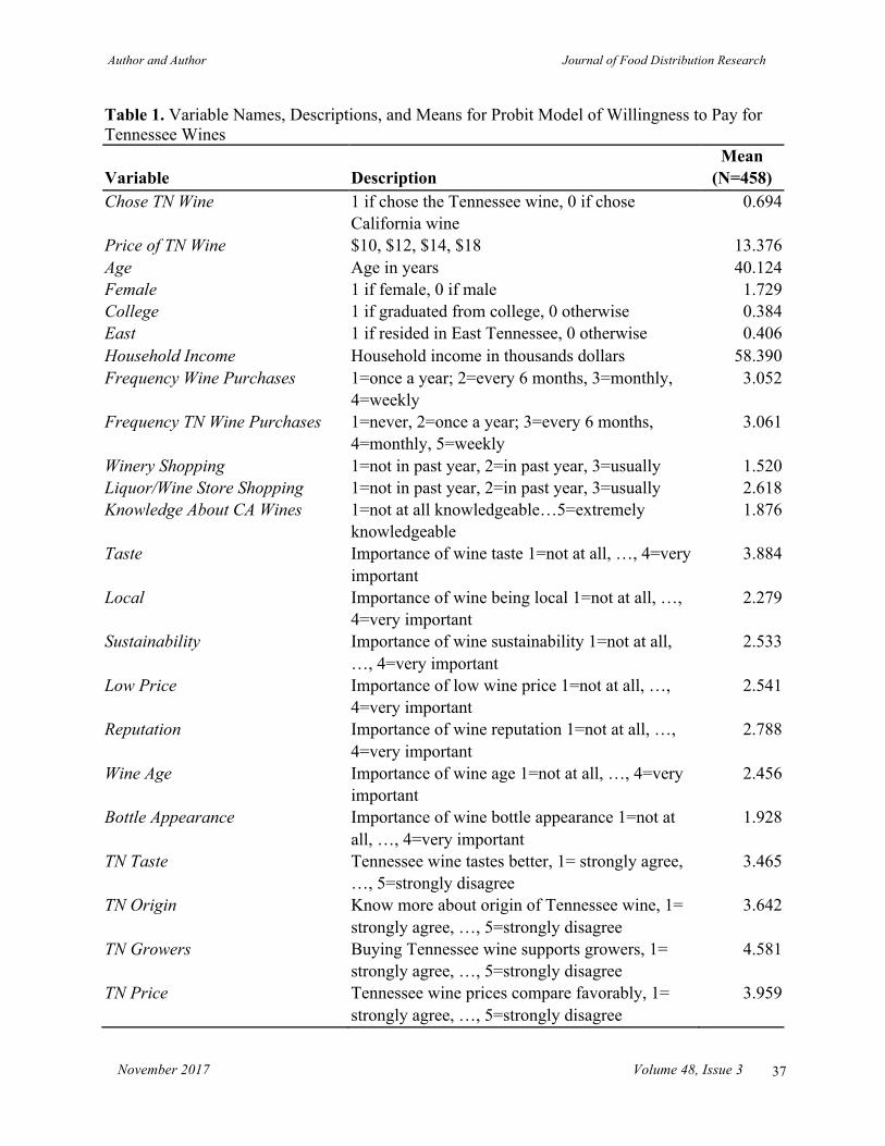
Author and Author Journal of Food Distribution Research
November 2017 Volume 48, Issue 3
37
Table 1. Variable Names, Descriptions, and Means for Probit Model of Willingness to Pay for Tennessee Wines
Variable Description Mean
(N=458) Chose TN Wine 1 if chose the Tennessee wine, 0 if chose
California wine 0.694
Price of TN Wine $10, $12, $14, $18 13.376 Age Age in years 40.124 Female 1 if female, 0 if male 1.729 College 1 if graduated from college, 0 otherwise 0.384 East 1 if resided in East Tennessee, 0 otherwise 0.406 Household Income Household income in thousands dollars 58.390 Frequency Wine Purchases 1=once a year; 2=every 6 months, 3=monthly,
4=weekly 3.052
Frequency TN Wine Purchases 1=never, 2=once a year; 3=every 6 months, 4=monthly, 5=weekly
3.061
Winery Shopping 1=not in past year, 2=in past year, 3=usually 1.520 Liquor/Wine Store Shopping 1=not in past year, 2=in past year, 3=usually 2.618 Knowledge About CA Wines 1=not at all knowledgeable…5=extremely
knowledgeable 1.876
Taste Importance of wine taste 1=not at all, …, 4=very important
3.884
Local Importance of wine being local 1=not at all, …, 4=very important
2.279
Sustainability Importance of wine sustainability 1=not at all, …, 4=very important
2.533
Low Price Importance of low wine price 1=not at all, …, 4=very important
2.541
Reputation Importance of wine reputation 1=not at all, …, 4=very important
2.788
Wine Age Importance of wine age 1=not at all, …, 4=very important
2.456
Bottle Appearance Importance of wine bottle appearance 1=not at all, …, 4=very important
1.928
TN Taste Tennessee wine tastes better, 1= strongly agree, …, 5=strongly disagree
3.465
TN Origin Know more about origin of Tennessee wine, 1= strongly agree, …, 5=strongly disagree
3.642
TN Growers Buying Tennessee wine supports growers, 1= strongly agree, …, 5=strongly disagree
4.581
TN Price Tennessee wine prices compare favorably, 1= strongly agree, …, 5=strongly disagree
3.959
Author and Author Journal of Food Distribution Research
November 2017 Volume 48, Issue 3
38
(6) 𝑆!,!∗ ≥ 𝑆!,!∗ . The explanatory variables (𝑍!) hypothesized to influence shopping location include respondent demographics, past wine shopping patterns, and attitudes about products (see variable descriptions in Table 2). The probability of anticipating shopping for Tennessee-labeled wine at particular outlets among wine shoppers who would purchase a Tennessee-labeled wine is estimated using a multivariate probit model:
(7) 𝑆!,!∗ = 𝜓ˊ𝑍!,! + 𝜖!,!, m = 1, ..., M
(8) 𝑆!,!∗ = 1 if 𝑆!,!∗ > 0 and 0 otherwise where 𝜖!,! are the random error terms distributed as multivariate normal, each with a mean of zero and covariance matrix V, where 𝑉!" = 1 if m=n or 𝐾!"𝐾!" 𝜌!" otherwise. Note that 𝜌!" are the correlations between error terms from equations m and n and 𝐾!" = 2𝑆!" − 1 for each i, k=1,…, M. The method of estimation is simulated maximum likelihood (Cappellari and Jenkins, 2003). Survey and Data
The survey panel was obtained through the online hosting service, Qualtrics, which recruited panelists who were Tennessee residents, 21 years or older, and wine consumers. A total of 500 survey responses was collected through the online survey platform in September of 2015. A copy of the survey instrument is available from the authors upon request. A map of counties in which respondents were located is shown in Figure 1.
Figure 1. Locations of the Tennessee Wine Survey Respondents
The survey was divided into several sections. In the first section, respondents were asked about their wine purchase and consumption habits, including questions about wine purchasing frequency and use of wine shopping venues (winery/vineyards or liquor/wine stores). The second section asked respondents to rate the importance of wine attributes such as taste/flavor, whether it was locally produced, price, sustainability, and its age.
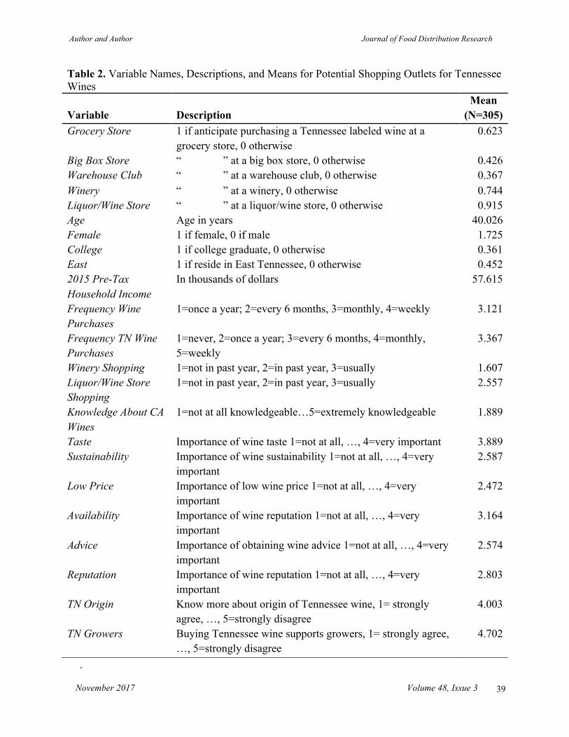
Author and Author Journal of Food Distribution Research
November 2017 Volume 48, Issue 3
39
Table 2. Variable Names, Descriptions, and Means for Potential Shopping Outlets for Tennessee Wines
Variable Description Mean
(N=305) Grocery Store 1 if anticipate purchasing a Tennessee labeled wine at a
grocery store, 0 otherwise 0.623
Big Box Store “ ” at a big box store, 0 otherwise 0.426 Warehouse Club “ ” at a warehouse club, 0 otherwise 0.367 Winery “ ” at a winery, 0 otherwise 0.744 Liquor/Wine Store “ ” at a liquor/wine store, 0 otherwise 0.915 Age Age in years 40.026 Female 1 if female, 0 if male 1.725 College 1 if college graduate, 0 otherwise 0.361 East 1 if reside in East Tennessee, 0 otherwise 0.452 2015 Pre-Tax Household Income
In thousands of dollars 57.615
Frequency Wine Purchases
1=once a year; 2=every 6 months, 3=monthly, 4=weekly 3.121
Frequency TN Wine Purchases
1=never, 2=once a year; 3=every 6 months, 4=monthly, 5=weekly
3.367
Winery Shopping 1=not in past year, 2=in past year, 3=usually 1.607 Liquor/Wine Store Shopping
1=not in past year, 2=in past year, 3=usually 2.557
Knowledge About CA Wines
1=not at all knowledgeable…5=extremely knowledgeable 1.889
Taste Importance of wine taste 1=not at all, …, 4=very important 3.889 Sustainability Importance of wine sustainability 1=not at all, …, 4=very
important 2.587
Low Price Importance of low wine price 1=not at all, …, 4=very important
2.472
Availability Importance of wine reputation 1=not at all, …, 4=very important
3.164
Advice Importance of obtaining wine advice 1=not at all, …, 4=very important
2.574
Reputation Importance of wine reputation 1=not at all, …, 4=very important
2.803
TN Origin Know more about origin of Tennessee wine, 1= strongly agree, …, 5=strongly disagree
4.003
TN Growers Buying Tennessee wine supports growers, 1= strongly agree, …, 5=strongly disagree
4.702
.

Author and Author Journal of Food Distribution Research
November 2017 Volume 48, Issue 3
40
In the third section, respondents were presented a choice experiment for Tennessee labeled wines (red or white) compared to California wines (red or white) depending on whether they indicated a red or white wine preference. A preference was randomly assigned if none had been indicated. Those who indicated they would purchase a Tennessee-labeled wine were asked about their anticipated shopping outlets for Tennessee wines, including newly available outlets (grocery stores, big box store, and warehouse clubs) and previously existing winery and liquor/wine store outlets. Respondents were asked whether they would likely purchase Tennessee wine at the following types of outlets: warehouse, winery, liquor/wine store, internet, grocery store, or big box store.
The fourth section asked respondents to rate the importance of factors influencing their decision of whether to select a Tennessee wine, including taste, patronage to local growers, and knowing more about the origin of the wine. The final survey section included demographic questions such as household income and respondents’ age, gender, and education level.
For the choice experiment, the sample was divided into two groups, depending on whether the consumer expressed a preference for red or white wines. If they expressed no preference, they were randomly assigned to a white or red wine experiment. Respondents were reminded of their budget constraint prior to answering the wine choice set question.4 The respondent was then presented a hypothetical buying scenario in which they were asked to choose between a “base” wine―represented by a California produced and labeled wine―and a Tennessee-produced and labeled wine. Figure 2 presents an example choice set for the Tennessee-labeled wine compared to the California-labeled wine. While the California wine price was held constant at $12 per bottle, the price of the Tennessee-labeled wine was allowed to vary across respondents, at prices of $10, $12, $14, and $18 per bottle. Note that the sample for the white wine experiment was divided into the four price levels, as was the red wine experiment, so each respondent was presented with one of the four price levels for the Tennessee wine.
In a 2014 survey of U.S. wine consumers, Thach and Olsen (2015) found that 35% of respondents spent $10–$15 per bottle, while 38% spent less than $10 and 27% spent more than $15. However, the Tennessee-labeled wine prices used in this study were similar to prices from an analysis of Virginia wines in which red and white Virginia wines were determined to be sold to either a super-premium ($10–$13.99 per bottle) or ultra-premium (>$14 per bottle) market segment (Ferreira and Ferreira, 2013). These price tiers were also found to be consistent with wines of comparable reputation in which niche branding and product loyalty were not considered in the pricing (Jarvis and Goodman, 2005). Additionally, a pretest using local participants was conducted to prior to fielding the online survey that, in part, examined pricing.
4 The reminder read “Before making your decision, consider your household budget. Consider thoroughly how the cost associated with your wine purchase will affect your budget, so that you are certain that you are actually willing to pay the cost associated with the alternative you choose.”

Author and Author Journal of Food Distribution Research
November 2017 Volume 48, Issue 3
41
Figure 2. Choice Set of Tennessee or California Wine Alternative A Alternative B Alternative C
Price $14.00/ bottle $12.00/ bottle
Label
I prefer
Figure 3. Percent Stating They Would Purchase the Tennessee-Labeled Wine Over the $12/Bottle California Wine.
82.54% 81.42%
66.67%
45.05%
0%
10%
20%
30%
40%
50%
60%
70%
80%
90%
$10.00 $12.00 $14.00 $18.00
Perc
ent
Cho
osin
g Te
nnes
see-
Lab
eled
W
ine
Ove
r th
e $1
2/B
ottle
Cal
iforn
ia
Win
e
Price of Tennessee-Labeled Wine (N=458)

Author and Author Journal of Food Distribution Research
November 2017 Volume 48, Issue 3
42
Results Willingness to Pay for Tennessee Red or White Wines A total of 458 respondents replied to the questions necessary for conducting the modeling analysis. Of the choice sets modeled, 52.6% of these were red wine choice sets. The LLR test comparing the model with the red wine choice set dummy interactions revealed that the hypothesis of the interaction coefficients being jointly 0 could not be rejected: –2(LLr–LLu)=28.53 < critical value of 𝜒!/!" !",!!.!"
! =35.17l. Hence the red and white dataset were estimated jointly. The estimated means for the variables included in the WTP model for the Tennessee-labeled wines are shown in Table 1. As shown in Table 1, 69.43% of the respondents indicated they would choose the Tennessee wine over the California wine. The percent of respondents choosing the Tennessee wine at each price level are displayed in Figure 3. Notably, at $10 per bottle, about 82.54% would choose the Tennessee wine. However, at $18 per bottle, this drops to 45.05%. The estimated probit model for the WTP for the Tennessee-labeled wines is presented in Table 3. As indicated by the LLR test against an intercept-only model, the estimated model is significant at the 95% confidence level. As expected, the sign on price of the Tennessee-labeled wine was significant and negative. The marginal effect shown in the fourth column suggests that, for each dollar increase in a Tennessee-labeled wine, the probability of choosing the Tennessee-labeled wine drops by 3.3%. Other variables that negatively influence the probability of choosing the Tennessee wine to a significant degree are Liquor/Wine Store Shopping, knowledge about California wines (Knowledge About CA Wines), importance of sustainability of wines (Sustainability), low wine price (Low Price), wine reputation (Reputation), and wine bottle appearance (Appear). These results suggest that low-price shoppers and reputation shoppers may be less willing to pay a premium for Tennessee-labeled wines. Holding all else constant, a person who usually shops for wine at liquor/wine stores was about 11% less likely to be willing to pay for Tennessee-labeled wine compared to a wine consumer who has not shopped for wine at a liquor/wine store in the past year. A person who is extremely knowledgeable about California wines was 15.9% less likely to choose the Tennessee wine compared to a person who considers themselves not knowledgeable about California wines. Price-concerned wine shoppers were more than 9% less likely to choose the Tennessee-labeled wine. Interestingly, wine consumers who were more concerned about sustainability and wine reputation were also less likely to select the Tennessee-labeled wine. This result could suggest a lack of knowledge about how Tennessee wine grapes are produced relative to California wines as well as beliefs that Tennessee-labeled wines do not have the same reputation as California wines. Variables with significantly positive influence included being from the eastern region of the state (East), household income (Household Income), respondent’s belief that Tennessee-produced wines taste better (TN Taste), the respondent knowing more about the origin of Tennessee wines (TN Origin), his or her belief that purchasing Tennessee wines helps local growers (TN Grower),

Author and Author Journal of Food Distribution Research
November 2017 Volume 48, Issue 3
43
Table 3. Estimated Probit Model for Willingness to Pay for Tennessee-Labeled Wine Variable Est. Coeff. Std. Err. Marg. Eff. Std. Err. Intercept 0.327 1.278 Price of TN Wine -0.151 0.026 *** -0.033 0.005 *** Age 0.009 0.006 0.002 0.001 Female -0.077 0.191 -0.017 0.041 College -0.208 0.180 -0.045 0.039 East 0.404 0.164 *** 0.087 0.035 *** Household Income 0.004 0.002 * 0.001 0.000 ** Frequency Wine Purchases -0.001 0.105 0.000 0.023 Frequency TN Wine Purchases 0.331 0.083 *** 0.071 0.017 *** Winery Shopping -0.046 0.138 -0.010 0.030 Liquor/Wine Store Shopping -0.256 0.135 ** -0.055 0.029 ** Knowledge About CA Wines -0.184 0.120 ** -0.040 0.026 ** Taste -0.165 0.249 -0.036 0.054 Local 0.215 0.103 ** 0.046 0.022 ** Sustainability -0.191 0.111 * -0.041 0.024 * Low Price -0.142 0.092 * -0.031 0.020 * Reputation -0.160 0.098 * -0.034 0.021 * Wine Age -0.002 0.109 0.000 0.024 Bottle Appearance -0.202 0.098 ** -0.044 0.021 ** Taste 0.360 0.096 *** 0.078 0.020 *** TN Origin 0.159 0.074 *** 0.034 0.016 *** TN Growers 0.227 0.111 ** 0.049 0.024 ** TN Price 0.233 0.081 *** 0.050 0.017 *** Percent Correctly Classified 83.84% Pseudo R2 0.3801 N (458) LLR Test (22 df)=214.32*** Mean WTP for Tennessee Wine=$18.27, LCL=$16.81, UCL=$20.91 Notes: *** indicates significance at 𝛼=0.01, ** at 𝛼=0.05, and * at 𝛼=0.15. believing that Tennessee wines were priced favorably (TN Price), and knowing that wines were local (Local). In addition, more frequent prior purchases of Tennessee-labeled wines (Frequency TN Wine Purchases) have a positive influence on the respondent choosing a Tennessee wine. The marginal effects show that wine consumers in eastern Tennessee are 8.7% more likely to choose Tennessee wine than consumers from other parts of the state. Each additional thousand dollars of household income increases the probability of selecting Tennessee wine by 0.1%. A wine consumer who already purchases a Tennessee-labeled wine weekly is 28.6% more likely to choose the Tennessee-labeled wine in the choice set than someone who has not purchased Tennessee-labeled wines in the past. Among reasons for selecting Tennessee wines, taste (TN
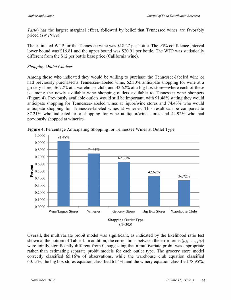
Author and Author Journal of Food Distribution Research
November 2017 Volume 48, Issue 3
44
Taste) has the largest marginal effect, followed by belief that Tennessee wines are favorably priced (TN Price). The estimated WTP for the Tennessee wine was $18.27 per bottle. The 95% confidence interval lower bound was $16.81 and the upper bound was $20.91 per bottle. The WTP was statistically different from the $12 per bottle base price (California wine). Shopping Outlet Choices Among those who indicated they would be willing to purchase the Tennessee-labeled wine or had previously purchased a Tennessee-labeled wine, 62.30% anticipate shopping for wine at a grocery store, 36.72% at a warehouse club, and 42.62% at a big box store―where each of these is among the newly available wine shopping outlets available to Tennessee wine shoppers (Figure 4). Previously available outlets would still be important, with 91.48% stating they would anticipate shopping for Tennessee-labeled wines at liquor/wine stores and 74.43% who would anticipate shopping for Tennessee-labeled wines at wineries. This result can be compared to 87.21% who indicated prior shopping for wine at liquor/wine stores and 44.92% who had previously shopped at wineries. Figure 4. Percentage Anticipating Shopping for Tennessee Wines at Outlet Type
Overall, the multivariate probit model was significant, as indicated by the likelihood ratio test shown at the bottom of Table 4. In addition, the correlations between the error terms (ρ21, …, ρ54) were jointly significantly different from 0, suggesting that a multivariate probit was appropriate rather than estimating separate probit models for each outlet type. The grocery store model correctly classified 65.16% of observations, while the warehouse club equation classified 60.15%, the big box stores equation classified 61.4%, and the winery equation classified 78.95%.
91.48%
74.43%
62.30%
42.62% 36.72%
0.0000
0.1000
0.2000
0.3000
0.4000
0.5000
0.6000
0.7000
0.8000
0.9000
1.0000
Wine/Liquor Stores Wineries Grocery Stores Big Box Stores Warehouse Clubs
Perc
ent
Shopping Outlet Type (N=305)
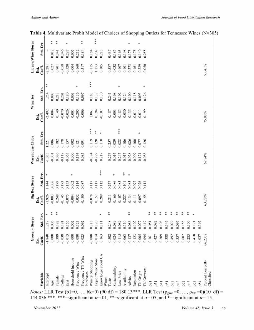
Author and Author Journal of Food Distribution Research
November 2017 Volume 48, Issue 3
45
Table 4. Multivariate Probit Model of Choices of Shopping Outlets for Tennessee Wines (N=305) L
iquo
r/W
ine
Stor
es
Std.
Err
. **
**
* **
***
* *
–2.
373
0.01
2 0.
341
0.34
6 0.
287
0.00
5 0.
212
0.18
4
0.18
4 0.
207
0.21
3
0.43
7 0.
185
0.16
3 0.
198
0.17
3 0.
175
0.14
0 0.
255
Est
. C
oeff
. -2
.281
0.
027
0.80
1 -0
.058
-0
.520
0.
004
-0.1
60
0.51
7
-0.1
15
1.15
3 0.
105
-0.5
87
-0.0
32
0.10
7 0.
101
-0.2
73
-0.1
61
0.22
9 -0
.050
95
.41%
Win
erie
s
Std.
Err
. **
* ***
* *
1.
254
0.00
7 0.
213
0.20
1 0.
180
0.00
3 0.
136
0.09
7
0.18
3 0.
137
0.13
0
0.24
1 0.
108
0.10
2 0.
124
0.10
0 0.
118
0.09
3 0.
126
Est
. C
oeff
.
-2.4
92
0.00
4 0.
140
-0.0
70
-0.0
26
0.00
1 -0
.205
0.
006
1.06
1 0.
194
-0.1
07
0.18
7 0.
003
-0.1
85
0.03
0 0.
135
-0.0
11
-0.0
11
0.19
9 75
.08%
War
ehou
se C
lubs
Std.
Err
. **
* **
* **
* *
1.
221
0.00
6 0.
182
0.17
8 0.
157
0.00
2 0.
121
0.09
1
0.11
9 0.
120
0.11
0
0.25
7 0.
089
0.08
8 0.
106
0.08
6 0.
100
0.07
7 0.
126
Est
. C
oeff
. -1
.035
-0
.001
0.
076
-0.1
18
-0.0
65
0.00
0 0.
134
0.08
5
-0.3
74
-0.2
79
0.21
7
0.27
7 0.
014
0.24
7 -0
.017
0.
028
-0.0
09
-0.1
21
-0.0
88
69.8
4%
Big
Box
Sto
res
Std.
Err
. * * ***
* **
*
1.
144
0.00
6 0.
179
0.17
3 0.
153
0.00
2 0.
114
0.08
7
0.11
7 0.
117
0.11
2
0.24
7 0.
086
0.08
5 0.
101
0.08
5 0.
097
0.07
6 0.
113
Est
. C
oeff
. -1
.926
-0
.003
0.
248
-0.1
45
-0.0
75
-0.0
04
0.05
2 -0
.100
-0.0
78
0.15
7 0.
289
0.21
1 -0
.166
0.
107
0.22
7 -0
.134
-0
.111
-0
.097
0.
155
63.2
8%
Gro
cery
Sto
res
Std.
Err
. * ** * **
* **
**
** * ** * **
** * ** * ** * ** * ** * *
1.
217
0.00
6 0.
182
0.18
1 0.
156
0.00
2 0.
123
0.09
2
0.11
8 0.
120
0.11
1
0.24
8 0.
089
0.08
9 0.
110
0.08
6 0.
102
0.07
7 0.
117
0.05
1 0.
082
0.10
3 0.
146
0.07
9 0.
097
0.15
5 0.
100
0.17
1 0.
192
Est
. C
oeff
.
-1.8
40
0.00
0 0.
389
-0.0
38
-0.0
13
0.00
0 -0
.080
-0
.023
-0.0
88
-0.0
14
0.16
3
0.50
2 -0
.024
0.
115
-0.0
63
-0.1
37
-0.1
23
-0.0
05
0.09
5 0.
761
0.42
7 0.
209
0.38
8 0.
492
0.33
7 0.
602
0.28
3 0.
418
-0.0
37
66.2
3%
Var
iabl
e In
terc
ept
Age
Fe
mal
e C
olle
ge
East
H
ouse
hold
Inco
me
Freq
uenc
y W
ine
Purc
hase
s Fr
eque
ncy
TN W
ine
Purc
hase
s W
iner
y Sh
oppi
ng
Liqu
or/W
ine
Stor
e Sh
oppi
ng
Kno
wle
dge
abou
t CA
W
ines
Ta
ste
Sust
aina
bilit
y Lo
w P
rice
Ava
ilabi
lity
Adv
ice
Rep
utat
ion
TN O
rigin
TN
Gro
wer
s ρ2
1 ρ3
1 ρ4
1 ρ5
1 ρ3
2 ρ4
2 ρ5
2 ρ4
3 ρ5
3 ρ5
4 Pe
rcen
t Cor
rect
ly
Cla
ssifi
ed
Notes: LLR Test (b1=0, …, bk=0) (90 df) = 180.13***. LLR Test (ρgwc =0, …, ρbw =0)(10 df) = 144.036 ***. ***=significant at 𝛼=.01, **=significant at 𝛼=.05, and *=significant at 𝛼=.15.

Author and Author Journal of Food Distribution Research
November 2017 Volume 48, Issue 3
46
The estimated marginal probability of consumers indicating they would shop for Tennessee-labeled wines at the grocery store was 60.06%, 37.43% at warehouse clubs, 43.07% at big box stores, and 72.67% at wineries. The model predicted that about 16.52% were willing to shop at any of these outlets, and less than 9.38% would shop at none of them. Age (Age) and female gender (Female) have positive effects on shopping for Tennessee-labeled wines in grocery stores and liquor/wine stores. Consumers located in the eastern part of the state (East) indicated that they would be less likely to shop for Tennessee-labeled wines at liquor/wine stores. Those making more frequent wine purchases (Frequency of Wine Purchases) indicated that they would be less likely to shop for Tennessee-labeled wines at wineries; however, those who more frequently purchase Tennessee-labeled wines indicated they would be more likely to shop for them at liquor/wine stores. Frequency of shopping for wines at any winery has a positive effect on shopping for Tennessee-labeled wines at wineries but a negative effect on shopping for Tennessee wines at warehouse clubs. A similar pattern holds for shopping frequency for wines at liquor/wine stores. Those interested in purchasing Tennessee-labeled wines and more knowledgeable about California wines were more likely to shop for Tennessee-labeled wines at grocery stores, big box stores, and warehouse clubs. This result may suggest that these shoppers would be comparing Tennessee-labeled wines with California wines where food products are sold. With respect to wine attributes, importance of taste positively affects shopping for wines at grocery stores, while importance of sustainability negatively influences shopping for Tennessee-labeled wines at big box stores. The results suggest that shoppers driven by low prices are more likely to shop for Tennessee-labeled wines at warehouse clubs but less likely to shop for them at wineries. Wine being readily available positively influences the likelihood that respondents would shop for Tennessee-labeled wines at big box stores, while wanting to obtain wine advice negatively influences the likelihood of shopping for Tennessee-labeled wines at grocery, big box, and liquor/wine stores. Knowing the origin of Tennessee wines positively influences shopping for those wines at liquor/wine stores, as expected. However, the importance of such knowledge negatively influences shopping for Tennessee wines at warehouse clubs. Furthermore, consumers who placed importance on Tennessee wines helping Tennessee grape growers are more likely to shop for Tennessee wines at wineries. The results suggest that lower income, convenience-oriented shoppers who are less concerned about sustainability and obtaining wine advice are more likely to shop for Tennessee wines at big box stores. Those shopping for Tennessee wines at grocery stores are more likely to be female and interested in wine taste but not concerned about obtaining advice. Warehouse club shoppers looking for Tennessee wines will likely be concerned with low price and be more knowledgeable about California wines but will be less likely to have already shopped for wines at wineries or liquor/wine stores and be less concerned about knowing where Tennessee wines are produced. The results suggest that winery shoppers and liquor/wine store shoppers will continue to shop for Tennessee wines at these locations. Those shopping for Tennessee wines at wineries are less concerned about low prices and more concerned about Tennessee wines benefiting local farmers. Liquor/wine store shoppers were more likely to be older, female, living in middle and west Tennessee, and more frequent Tennessee wine consumers who are concerned about where Tennessee wines come from.
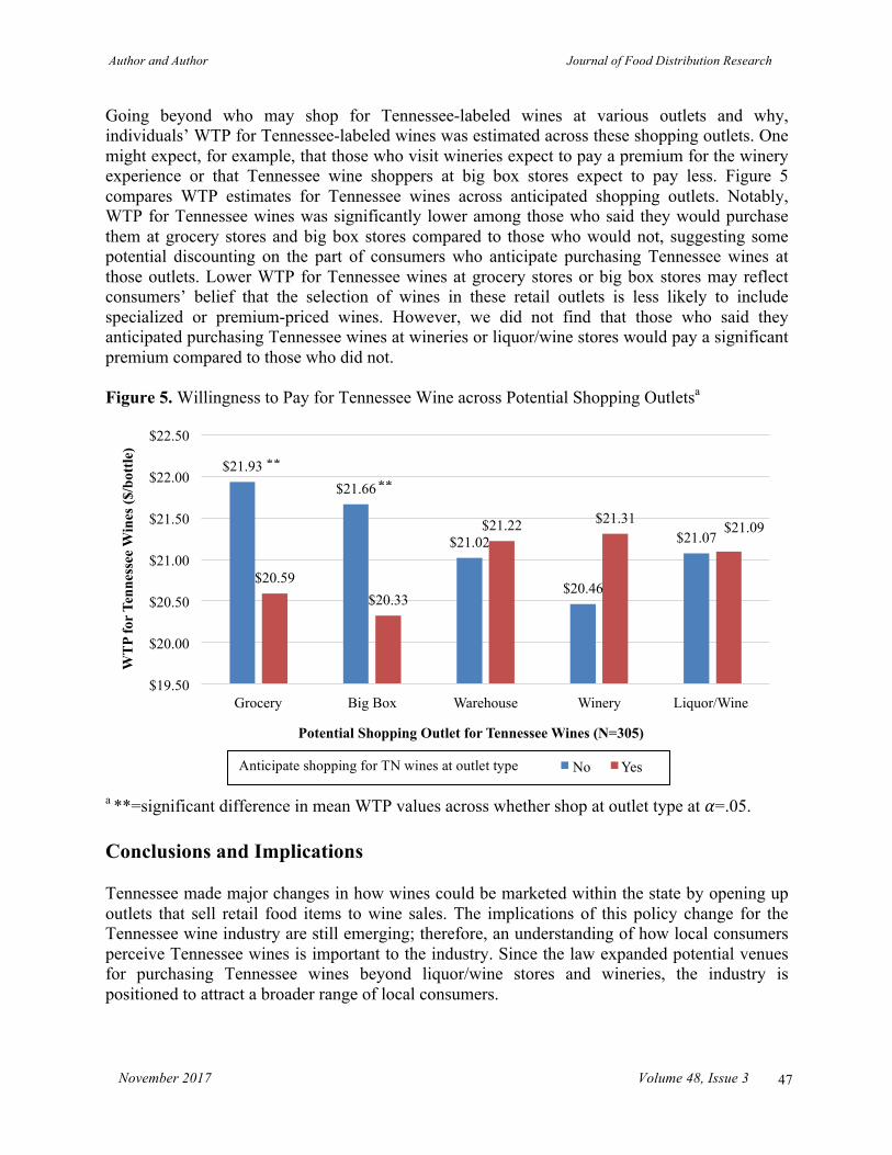
Author and Author Journal of Food Distribution Research
November 2017 Volume 48, Issue 3
47
Going beyond who may shop for Tennessee-labeled wines at various outlets and why, individuals’ WTP for Tennessee-labeled wines was estimated across these shopping outlets. One might expect, for example, that those who visit wineries expect to pay a premium for the winery experience or that Tennessee wine shoppers at big box stores expect to pay less. Figure 5 compares WTP estimates for Tennessee wines across anticipated shopping outlets. Notably, WTP for Tennessee wines was significantly lower among those who said they would purchase them at grocery stores and big box stores compared to those who would not, suggesting some potential discounting on the part of consumers who anticipate purchasing Tennessee wines at those outlets. Lower WTP for Tennessee wines at grocery stores or big box stores may reflect consumers’ belief that the selection of wines in these retail outlets is less likely to include specialized or premium-priced wines. However, we did not find that those who said they anticipated purchasing Tennessee wines at wineries or liquor/wine stores would pay a significant premium compared to those who did not. Figure 5. Willingness to Pay for Tennessee Wine across Potential Shopping Outletsa
a **=significant difference in mean WTP values across whether shop at outlet type at 𝛼=.05. Conclusions and Implications Tennessee made major changes in how wines could be marketed within the state by opening up outlets that sell retail food items to wine sales. The implications of this policy change for the Tennessee wine industry are still emerging; therefore, an understanding of how local consumers perceive Tennessee wines is important to the industry. Since the law expanded potential venues for purchasing Tennessee wines beyond liquor/wine stores and wineries, the industry is positioned to attract a broader range of local consumers.
$21.93 $21.66
$21.02
$20.46
$21.07
$20.59 $20.33
$21.22 $21.31 $21.09
$19.50
$20.00
$20.50
$21.00
$21.50
$22.00
$22.50
Grocery Big Box Warehouse Winery Liquor/Wine
WT
P fo
r Ten
ness
ee W
ines
($/b
ottle
)
Potential Shopping Outlet for Tennessee Wines (N=305)
No Yes Anticipate shopping for TN wines at outlet type
** **

Author and Author Journal of Food Distribution Research
November 2017 Volume 48, Issue 3
48
A choice set experiment revealed that some consumers who stated that they would choose Tennessee-labeled wine still anticipated purchasing Tennessee wines at wineries and liquor/wine stores, while others indicated a willingness to buy them at newly available outlets (grocery stores, big box stores, and warehouse clubs). Consumer demographics and attitudes play significant roles in where Tennessee wine shoppers would expect to purchase local wines. Older females who are taste-conscious shoppers but don’t feel a strong need for advice on buying wine and consider themselves more knowledgeable about California wines are more likely to shop for Tennessee wines at the grocery store. Big box store shoppers tend to be lower-income consumers who value the convenience of shopping for Tennessee wines at these venues but don’t feel a strong need for information about wine and consider themselves more knowledgeable about California wines. Warehouse shoppers value low prices but, again, consider themselves more knowledgeable about California wines. Interestingly, prior winery and liquor/wine store shopping behavior for Tennessee wines were both negatively related to shopping for those wines at warehouse clubs. One possibility is that warehouse shoppers may have been more likely to cross state lines to purchase wines in bulk from out-of-state warehouse clubs. Past purchase patterns for wines at wineries and liquor/wine stores had strong influences on continued shopping for Tennessee wines at these same outlets. Wineries proved to be the only outlet where the role of Tennessee wines in helping local farmers appeared to influence anticipated shopping, suggesting these consumers still view the winery as strongly tied to wine grape growers. Even with access to larger grocery retail, big box, and warehouse club chains, it may be difficult to change shopping preference for local wines, since differences in WTP for local wines at these outlets are still unknown. In these locations, consumers could face a variety of wine choices (including California wines, about which many consumers consider themselves to be more knowledgeable). The results from this study suggest that consumers who anticipated purchasing Tennessee wines at grocery stores and big box stores had lower WTP values than those who did not intend to use these outlets. At the time of our survey, only wineries and liquor/wine stores were available to wine shoppers in Tennessee. Therefore, no pricing data were available for Tennessee wines in food-retail facilities at the time of the survey, which would have allowed a price comparison to wines sold at wineries and liquor/wine stores. As Tennessee wines can now be sold in these outlets, future research might examine the extent to which local wines are being sold in food-retailing outlets. Future research might also examine the pricing of wines across food-retailing outlets compared to wineries and liquor/wine stores as well as consumer expectations about pricing and marketing of local wines at food-retailing outlets. Acknowledgments Support for the research presented in this article was provided by the Tennessee Farm Winegrowers Alliance, U.S. Department of Agriculture Rural Development-Tennessee Office, and the Tennessee Department of Agriculture. References Balter, E. 2017. “Wine Legislation Roundup: A Consumer's Guide to 2017 State Politics.”
Wine Spectator, March 28. Available online: http://www.winespectator.com/webfeature/show/id/Wine-Legislation-Roundup-2017
Author and Author Journal of Food Distribution Research
November 2017 Volume 48, Issue 3
49
Beames, G. 2003. “The Rock, the Reef and the Grape: The Challenges of Developing Wine Tourism in Regional Australia.” Journal of Vacation Marketing 9:205–212.
Brooks, E. 2001. “Counties as Brands: International Trade in Wine.” Paper presented at the Conference of the Vineyard Data Quantification Society, St. Helena, CA, May 21–22.
Bruwer, J., and I. Lesschaeve. 2012. “Wine Tourists’ Destination Region Brand Image Perception and Antecedents: Conceptualization of a Winescape Framework.” Journal of Travel and Tourism Marketing 29:611–628.
Cappellari, L., and S. Jenkins. 2003. “Multivariate Probit Regression Using Simulated Maximum Likelihood,” STATA Journal 3(3):278–294.
Charters, S., and J. Ali-Knight. 2002. “Who Is The Wine Tourist?” Tourism Management 23(3):311–319.
Corsi, A., J. Cohen, and L. Lockshin. 2014. “Store Image Perception of Retail Outlets for Wine in China.” Paper presented at the Academy of Wine Business Research 8th International Conference, Geisenheim, Germany, June 28–30. Available online http://academyofwinebusiness.com/wp-content/uploads/2014/07/CH01_Corsi_Armando.pdf
Ferreira, J., and G. Ferreira. “Pricing Strategies for Virginia Wineries.” AAEC Extension Update, Virginia Tech University. Available online: http://news.cals.vt.edu/fbm-update/2013/08/08/pricing-strategies-for-virginia-wineries/
Getz, D., and G. Brown. 2006. “Critical Success Factors for Wine Tourism Regions: A Demand Analysis.” Tourism Management 27(1):146–158.
Greene, W. 2011. Econometric Analysis, 7th ed. Upper Saddle River, NJ: Prentice Hall.
Jarvis, W., and S. Goodman. 2005. “Effective Marketing of Small Brands: Niche Positions, Attribute Loyalty and Small Brands.” Journal of Product and Brand Management 14(5):292–299.
Krinsky, I., and A. Robb. 1986. “On Approximating the Statistical Properties of Elasticities.” Revue of Economics and Statistics 68:715–719.
Kolyesnikova, N., T. Dodd, and D. Duhan. 2008."Consumer Attitudes towards Local Wines in an Emerging Region: A Segmentation Approach." International Journal of Wine Business Research 20(4):321–334.
Marcum, E. 2017. “Tennessee Grocery Stores Say Wine Sales a Success.” USA Today Network – Tennessee, March 17. Available online: https://www.usatoday.com/story/money/business/2017/03/17/tennessee-grocery-stores-say-wine-sales-success/99211156/
McFadden, D. 1974. Conditional Logit Analysis of Qualitative Choice Behavior. In P. Zarembka, ed. Frontiers in Econometrics. New York: Academic Press, pp. 105–142.
Nielsen Company. 2015. “Grapes of Worth: How Supermarkets are Becoming Local Wine Shops” Newswire, February 19. Available online: http://www.nielsen.com/us/en/insights/news/2015/grapes-of-worth-how-supermarkets-are-becoming-local-wine-shops.html
Author and Author Journal of Food Distribution Research
November 2017 Volume 48, Issue 3
50
Olsen, J., T. Atkin. L. Thach, and S. Cuellar. 2015."Variety Seeking by Wine Consumers in the Southern States of the US.” International Journal of Wine Business Research 27(4): 260–280.
O’Neill, M., and S. Charters. 2000. “Service Quality at the Cellar Door: Implications for Western Australia’s Developing Wine Tourism Industry.” Managing Service Quality: An International Journal 10(2):112–122.
Scarpa R., M. Thiene, and L. Galletto. 2009. “Consumers’ WTP for Wine with Certified Origin: Preliminary Results from Latent Classes Based on Attitudinal Response.” Journal of Food Products Marketing 15(3):231–248.
Soulek, K., T. Dodd, and N. Velikova. 2016. “Consumer Attitudes toward Texas Wine: A Comparative Report 2006–2016.” Texas Wine Marketing Research Institute, College of Human Sciences, Texas Tech University, November. Available online: http://www.depts.ttu.edu/hs/texaswine/docs/Consumer-Attitudes-Towards-Texas-Wine.pdf
Steiner, B. 2000. “In Vino Veritas: Does Origin Truly Matter? The Socio-Economics of Origin Labelled Products in Agri-Food Supply Chains: Spatial, Institutional and Coordination Aspects.” Actes et Communications 17:100–115.
Tennessee Legislature. 2014. Senate Bill 837, An Act to amend Tennessee Code Annotated, Title 2 and Title 57, Relative to Alcoholic Beverages. 108th Tennessee General Assembly. Available online: http://www.capitol.tn.gov/Bills/108/Bill/SB0837.pdf
Thach, L. and K. Chang. 2015. “2015 Survey of American Wine Consumer Preferences.” Wine Business, November 11. Available online: https://www.winebusiness.com/news/?go=getArticle&dataid=160722
Thach, L., and J. Olsen. 2015. “Profiling the High Frequency Wine Consumer by Price Segmentation in the US Market.” Wine Economics and Policy 4(1):53–59.
Thiene, M., L. Galletto, R. Scarpa, and V. Boatto. 2013. “Determinants of WTP for Prosecco Wine.” British Food Journal 115(2):279–299
U.S. Census Bureau. 2013 County Business Patterns. Washington, DC: U.S. Census Bureau. Available online: https://www.census.gov/data/datasets/2013/econ/cbp/2013-cbp.html
Wine Institute. 2017a. “US/California Wine Production.” Available online: https://www.wineinstitute.org/resources/statistics/article83
Wine Institute. 2017b. “2016 California Wine Sales in U.S. Hit New Record: 238 Million Cases with Retail Value of $34.1 Billion.” Available online: http://www.wineinstitute.org/resources/pressroom/05012017
Woods, T., X. Deng, L. Nogueira, and S. Yang. 2015. “Local Wine Expenditure Determinants in the Northern Appalachian States.” Journal of Food Distribution Research 46(2):30–50.
Woods, T., L. Noguiera, and S. Yang. 2013. “Linking Wine Consumers to the Consumption of Local Wines and Winery Visits in the Northern Appalachian States.” International Food and Agribusiness Management Review 16(4):181–205.

Journal of Food Distribution Research Volume 48, Issue 3
November 2017 Volume 48, Issue 3
51
Understanding Spending Habits and Buying Behavior of the
American Muslim Community: A Pilot Study
Oral Capps, Jr.,a! Asma Ahad,b and Peter S. Muranoc
aExecutive Professor and Regents Professor, Department of Agricultural Economics
Texas A&M University 600 John Kimbrough Blvd, Suite 371, College Station, TX 77843 USA
bDirector of Halal Market Development,
Islamic Food and Nutrition Council of America 777 Busse Highway, Park Ridge, IL 60068 USA
cAssociate Professor, Department of Nutrition and Food Science
Texas A&M University 188 Cater-Mattil, College Station, TX 77843 USA
Abstract
This study provides a baseline for the spending habits and buying preferences of American Muslims lacking in the extant literature. We examine American Muslims’ food and beverage spending habits and buying behaviors with regard to halal products using a survey of 195 individuals from the Chicago metropolitan area and a discrete choice modeling framework. The chief drivers in the decision to purchase food and beverage items were the purchase of halal beef, the amount spent weekly in grocery stores, the frequency of hosting Ramadan, household income and size, and ethnicity (in that order). Keywords: American Muslims, food and beverage choices, probit/logit analysis
!Corresponding author: Tel: (979) 845-8492
Email: [email protected]
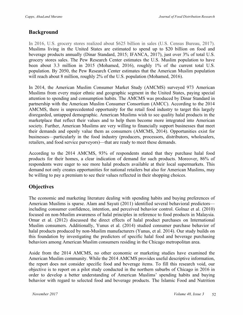
Capps, Ahad,and Murano Journal of Food Distribution Research
November 2017 Volume 48, Issue 3
52
Background In 2016, U.S. grocery stores realized about $625 billion in sales (U.S. Census Bureau, 2017). Muslims living in the United States are estimated to spend up to $20 billion on food and beverage products annually (Dinar Standard, 2015; IFANCA, 2017), just over 3% of total U.S. grocery stores sales. The Pew Research Center estimates the U.S. Muslim population to have been about 3.3 million in 2015 (Mohamed, 2016), roughly 1% of the current total U.S. population. By 2050, the Pew Research Center estimates that the American Muslim population will reach about 8 million, roughly 2% of the U.S. population (Mohamed, 2016). In 2014, the American Muslim Consumer Market Study (AMCMS) surveyed 973 American Muslims from every major ethnic and geographic segment in the United States, paying special attention to spending and consumption habits. The AMCMS was produced by Dinar Standard in partnership with the American Muslim Consumer Consortium (AMCC). According to the 2014 AMCMS, there is unprecedented opportunity for the retail food industry to target this largely disregarded, untapped demographic. American Muslims wish to see quality halal products in the marketplace that reflect their values and to help them become more integrated into American society. Further, American Muslims are very willing to financially support businesses that meet their demands and openly value them as consumers (AMCMS, 2014). Opportunities exist for businesses—particularly in the food industry (producers, processors, distributors, wholesalers, retailers, and food service purveyors)—that are ready to meet these demands. According to the 2014 AMCMS, 93% of respondents stated that they purchase halal food products for their homes, a clear indication of demand for such products. Moreover, 86% of respondents were eager to see more halal products available at their local supermarkets. This demand not only creates opportunities for national retailers but also for American Muslims, may be willing to pay a premium to see their values reflected in their shopping choices. Objectives The economic and marketing literature dealing with spending habits and buying preferences of American Muslims is sparse. Alam and Sayuti (2011) identified several behavioral predictors—including consumer confidence, intention, and perceived behavior control. Golnaz et al. (2010) focused on non-Muslim awareness of halal principles in reference to food products in Malaysia. Omar et al. (2012) discussed the direct effects of halal product purchases on International Muslim consumers. Additionally, Yunus et al. (2014) studied consumer purchase behavior of halal products produced by non-Muslim manufacturers (Yunus, et al. 2014). Our study builds on this foundation by investigating the predictors of specific halal food and beverage purchasing behaviors among American Muslim consumers residing in the Chicago metropolitan area. Aside from the 2014 AMCMS, no other economic or marketing studies have examined the American Muslim community. While the 2014 AMCMS provides useful descriptive information, the report does not consider specific food and beverage items. To fill this research void, our objective is to report on a pilot study conducted in the northern suburbs of Chicago in 2016 in order to develop a better understanding of American Muslims’ spending habits and buying behavior with regard to selected food and beverage products. The Islamic Food and Nutrition
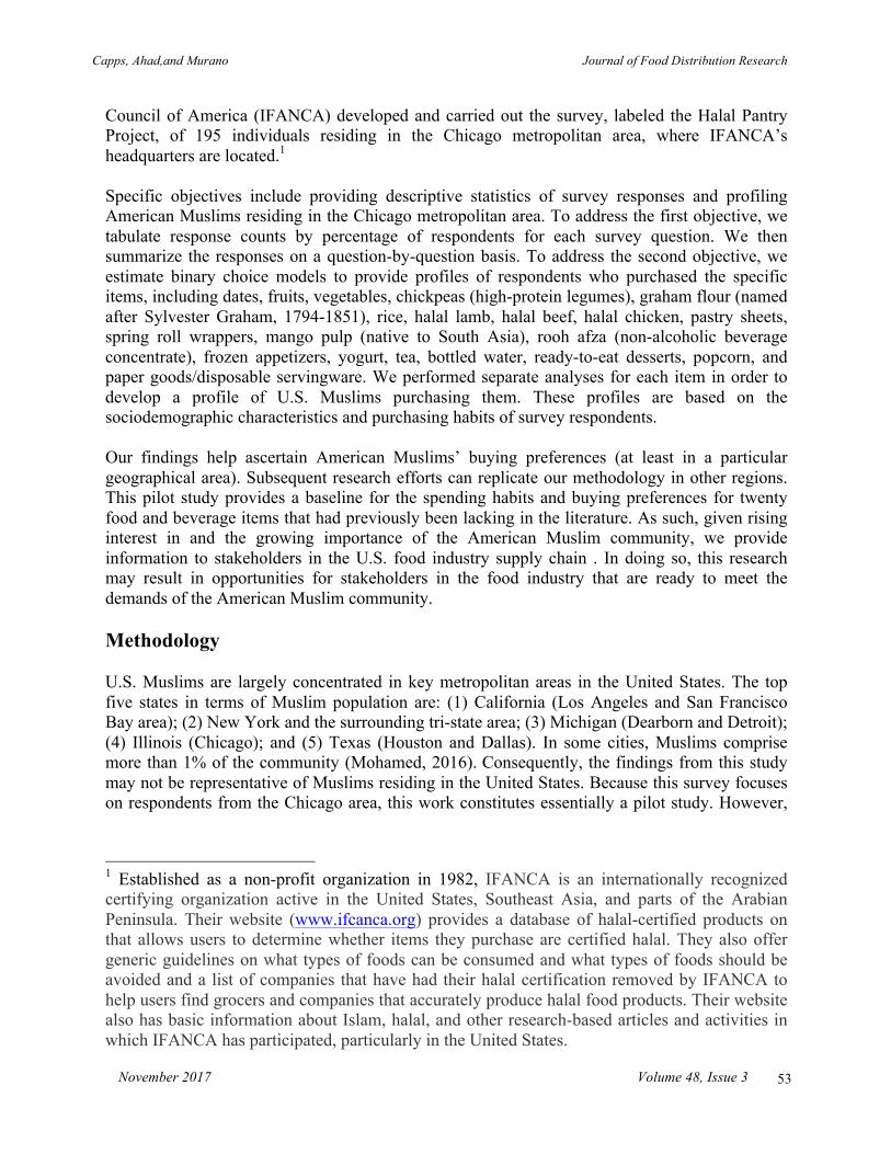
Capps, Ahad,and Murano Journal of Food Distribution Research
November 2017 Volume 48, Issue 3
53
Council of America (IFANCA) developed and carried out the survey, labeled the Halal Pantry Project, of 195 individuals residing in the Chicago metropolitan area, where IFANCA’s headquarters are located.1 Specific objectives include providing descriptive statistics of survey responses and profiling American Muslims residing in the Chicago metropolitan area. To address the first objective, we tabulate response counts by percentage of respondents for each survey question. We then summarize the responses on a question-by-question basis. To address the second objective, we estimate binary choice models to provide profiles of respondents who purchased the specific items, including dates, fruits, vegetables, chickpeas (high-protein legumes), graham flour (named after Sylvester Graham, 1794-1851), rice, halal lamb, halal beef, halal chicken, pastry sheets, spring roll wrappers, mango pulp (native to South Asia), rooh afza (non-alcoholic beverage concentrate), frozen appetizers, yogurt, tea, bottled water, ready-to-eat desserts, popcorn, and paper goods/disposable servingware. We performed separate analyses for each item in order to develop a profile of U.S. Muslims purchasing them. These profiles are based on the sociodemographic characteristics and purchasing habits of survey respondents. Our findings help ascertain American Muslims’ buying preferences (at least in a particular geographical area). Subsequent research efforts can replicate our methodology in other regions. This pilot study provides a baseline for the spending habits and buying preferences for twenty food and beverage items that had previously been lacking in the literature. As such, given rising interest in and the growing importance of the American Muslim community, we provide information to stakeholders in the U.S. food industry supply chain . In doing so, this research may result in opportunities for stakeholders in the food industry that are ready to meet the demands of the American Muslim community. Methodology U.S. Muslims are largely concentrated in key metropolitan areas in the United States. The top five states in terms of Muslim population are: (1) California (Los Angeles and San Francisco Bay area); (2) New York and the surrounding tri-state area; (3) Michigan (Dearborn and Detroit); (4) Illinois (Chicago); and (5) Texas (Houston and Dallas). In some cities, Muslims comprise more than 1% of the community (Mohamed, 2016). Consequently, the findings from this study may not be representative of Muslims residing in the United States. Because this survey focuses on respondents from the Chicago area, this work constitutes essentially a pilot study. However,
1 Established as a non-profit organization in 1982, IFANCA is an internationally recognized certifying organization active in the United States, Southeast Asia, and parts of the Arabian Peninsula. Their website (www.ifcanca.org) provides a database of halal-certified products on that allows users to determine whether items they purchase are certified halal. They also offer generic guidelines on what types of foods can be consumed and what types of foods should be avoided and a list of companies that have had their halal certification removed by IFANCA to help users find grocers and companies that accurately produce halal food products. Their website also has basic information about Islam, halal, and other research-based articles and activities in which IFANCA has participated, particularly in the United States.
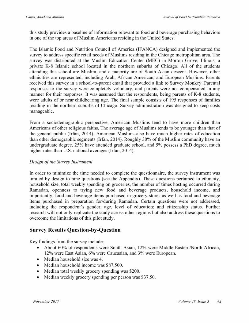
Capps, Ahad,and Murano Journal of Food Distribution Research
November 2017 Volume 48, Issue 3
54
this study provides a baseline of information relevant to food and beverage purchasing behaviors in one of the top areas of Muslim Americans residing in the United States. The Islamic Food and Nutrition Council of America (IFANCA) designed and implemented the survey to address specific retail needs of Muslims residing in the Chicago metropolitan area. The survey was distributed at the Muslim Education Center (MEC) in Morton Grove, Illinois, a private K-8 Islamic school located in the northern suburbs of Chicago. All of the students attending this school are Muslim, and a majority are of South Asian descent. However, other ethnicities are represented, including Arab, African American, and European Muslims. Parents received this survey in a school-to-parent email that provided a link to Survey Monkey. Parental responses to the survey were completely voluntary, and parents were not compensated in any manner for their responses. It was assumed that the respondents, being parents of K-8 students, were adults of or near childbearing age. The final sample consists of 195 responses of families residing in the northern suburbs of Chicago. Survey administration was designed to keep costs manageable. From a sociodemographic perspective, American Muslims tend to have more children than Americans of other religious faiths. The average age of Muslims tends to be younger than that of the general public (Irfan, 2014). American Muslims also have much higher rates of education than other demographic segments (Irfan, 2014). Roughly 30% of the Muslim community have an undergraduate degree, 25% have attended graduate school, and 5% possess a PhD degree, much higher rates than U.S. national averages (Irfan, 2014). Design of the Survey Instrument In order to minimize the time needed to complete the questionnaire, the survey instrument was limited by design to nine questions (see the Appendix). These questions pertained to ethnicity, household size, total weekly spending on groceries, the number of times hosting occurred during Ramadan, openness to trying new food and beverage products, household income, and importantly, food and beverage items purchased in grocery stores as well as food and beverage items purchased in preparation for/during Ramadan. Certain questions were not addressed, including the respondent’s gender, age, level of education; and citizenship status. Further research will not only replicate the study across other regions but also address these questions to overcome the limitations of this pilot study. Survey Results Question-by-Question Key findings from the survey include:
• About 60% of respondents were South Asian, 12% were Middle Eastern/North African, 12% were East Asian, 6% were Caucasian, and 3% were European.
• Median household size was 4. • Median household income was $87,500. • Median total weekly grocery spending was $200. • Median weekly grocery spending per person was $37.50.

Capps, Ahad,and Murano Journal of Food Distribution Research
November 2017 Volume 48, Issue 3
55
• 62% of respondents spent more on groceries during Ramadan than in other months.2 • Among those who spent more on groceries during Ramadan, the median additional
amount spent was $200.2 • Close to 60% of respondents hosted 1 to 4 times during Ramadan, while close to 30% did
not host at all.2 • About 95% of respondents were open to trying new food and beverage products. • The most popular food and beverage items in terms of the percentage of respondents
purchasing were (1) fruits (98%); (2) vegetables (97%); (3) rice (93%); (4) halal chicken (92%); (5) yogurt (88%); (6) tea (84%); (7) halal beef (81%); (8) halal lamb (68%); (9) chickpeas (58%); (10) bottled water (54%); and (11) popcorn (53%).
• The least popular food and beverage items in terms of the percentage of respondents purchasing were: (1) rooh afza (15%); (2) spring roll wrappers (27%); (3) mango pulp (28%); (4) pastry sheets (35%); (5) graham flour (37%); (6) frozen appetizers (37%); (7) dates (41%); and (8) ready-to-eat desserts (45%).
Figures 1–10 present survey responses details.
2 Ramadan typically falls between late May and late June and lasts approximately 30 days. Fasting during Ramadan, called sawm, is one of the five pillars of Islam that are important to Muslims. The physical fast takes place daily from sunrise to sunset. Before dawn, those observing Ramadan will gather for a pre-fast meal called suhoor; at dusk, the fast will be broken with a meal called iftar. Both meals may be communal, but the iftar is an especially social affair when extended families gather to eat and mosques welcome the needy with food. Focusing on Ramadan allows us to capture potential differences in purchases of selected foods and beverages during and outside this period of time.
Caucasian 6% African American
2%
Middle Eastern/North African
12%
South Asian 57%
East Asian 12%
African 0%
Hispanic 1%
European 3%
Other 6%
N/A 1%
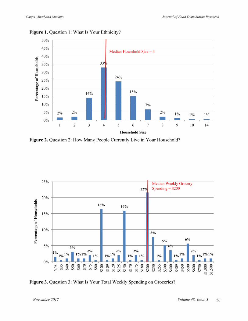
Capps, Ahad,and Murano Journal of Food Distribution Research
November 2017 Volume 48, Issue 3
56
Figure 1. Question 1: What Is Your Ethnicity?
Figure 2. Question 2: How Many People Currently Live in Your Household?
Figure 3. Question 3: What Is Your Total Weekly Spending on Groceries?
2% 2%
14%
33%
24%
15%
7%
2% 1% 1% 1% 0%
5%
10%
15%
20%
25%
30%
35%
40%
45%
50%
1 2 3 4 5 6 7 8 9 10 14
Perc
enta
ge o
f Hou
seho
lds
Household Size
2% 1% 1%
3%
1% 1% 2%
1%
16%
1% 1% 2%
16%
1% 2%
1%
22%
8%
1%
5% 4%
1% 1%
6%
2% 1% 1% 1%
0%
5%
10%
15%
20%
25%
N/A
$3
5 $4
0 $5
0 $6
0 $7
0 $7
5 $8
0 $1
00
$109
$1
20
$125
$1
50
$170
$1
75
$180
$2
00
$250
$2
55
$300
$4
00
$409
$4
50
$500
$6
00
$750
$1
,000
$1
,500
Perc
enta
ge o
f Hou
seho
lds
Median Weekly Grocery Spending = $200
Median Household Size = 4
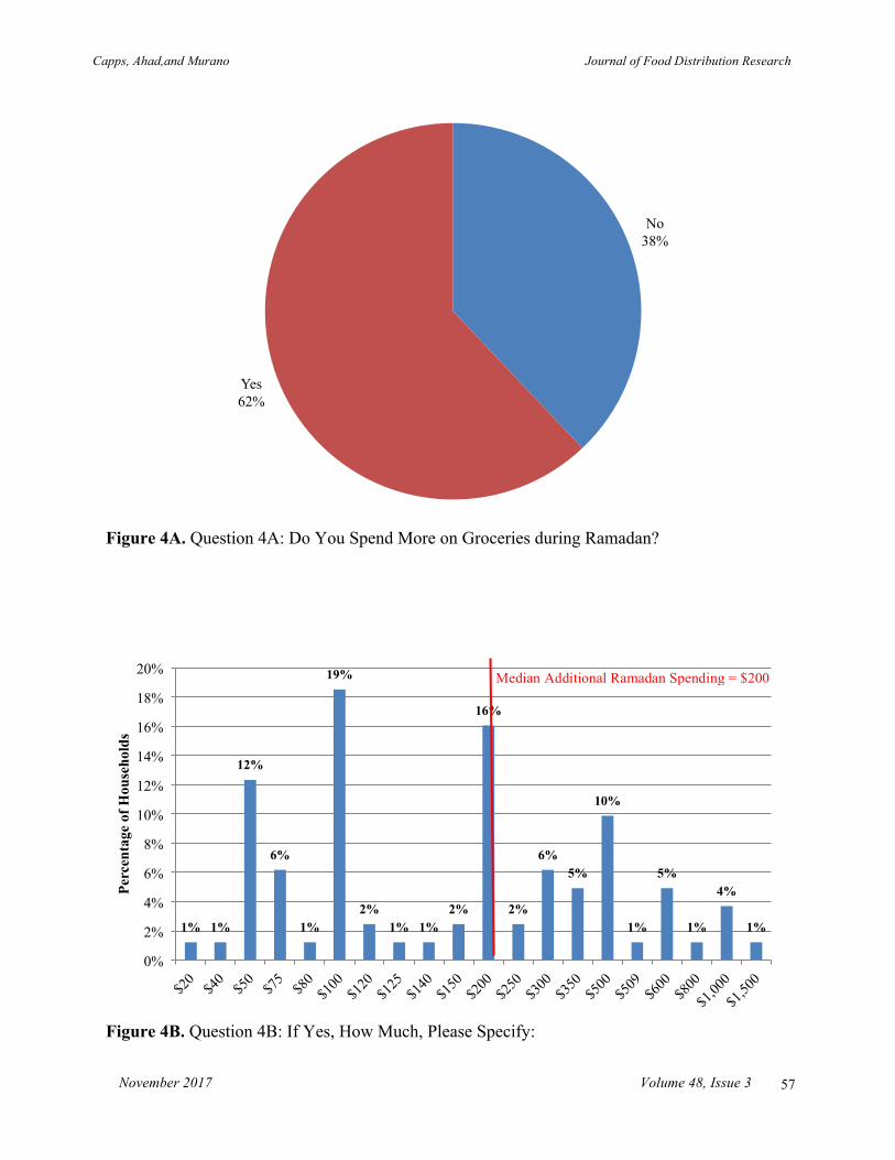
Capps, Ahad,and Murano Journal of Food Distribution Research
November 2017 Volume 48, Issue 3
57
Figure 4A. Question 4A: Do You Spend More on Groceries during Ramadan?
Figure 4B. Question 4B: If Yes, How Much, Please Specify:
No 38%
Yes 62%
1% 1%
12%
6%
1%
19%
2% 1% 1%
2%
16%
2%
6% 5%
10%
1%
5%
1%
4%
1%
0%
2%
4%
6%
8%
10%
12%
14%
16%
18%
20%
Perc
enta
ge o
f Hou
seho
lds
Median Additional Ramadan Spending = $200

Capps, Ahad,and Murano Journal of Food Distribution Research
November 2017 Volume 48, Issue 3
58
Figure 5. Question 5: How Many Times Do You Host during the Month of Ramadan?
Figure 6. Question 6: I Am Open to Trying New Food and Beverage Items?
28%
17% 19%
13%
9%
6%
2% 1%
2% 3%
1%
0%
5%
10%
15%
20%
25%
30%
0 1 2 3 4 5 6 7 8 10 12
Perc
enta
ge o
f Hou
seho
lds
No, 5%
Yes, 94%
N/A, 1%
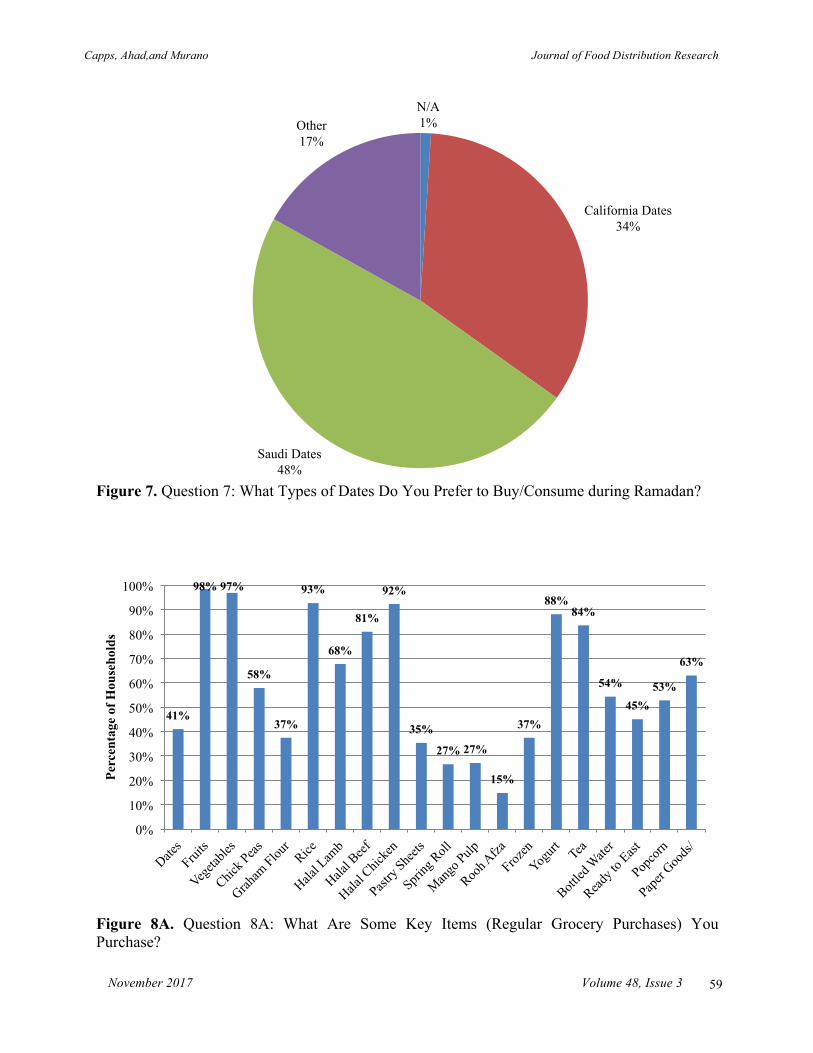
Capps, Ahad,and Murano Journal of Food Distribution Research
November 2017 Volume 48, Issue 3
59
Figure 7. Question 7: What Types of Dates Do You Prefer to Buy/Consume during Ramadan?
Figure 8A. Question 8A: What Are Some Key Items (Regular Grocery Purchases) You Purchase?
N/A 1%
California Dates 34%
Saudi Dates 48%
Other 17%
41%
98% 97%
58%
37%
93%
68%
81%
92%
35%
27% 27%
15%
37%
88% 84%
54%
45% 53%
63%
0%
10%
20%
30%
40%
50%
60%
70%
80%
90%
100%
Perc
enta
ge o
f Hou
seho
lds
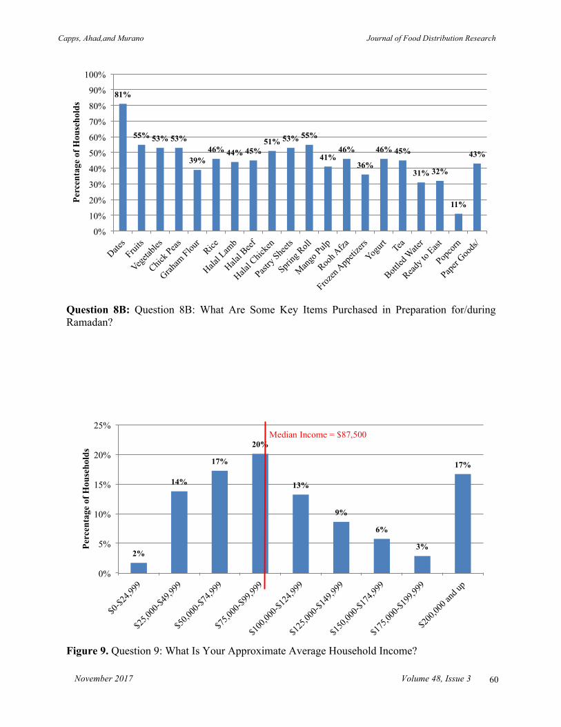
Capps, Ahad,and Murano Journal of Food Distribution Research
November 2017 Volume 48, Issue 3
60
Question 8B: Question 8B: What Are Some Key Items Purchased in Preparation for/during Ramadan?
Figure 9. Question 9: What Is Your Approximate Average Household Income?
81%
55% 53% 53%
39% 46% 44% 45%
51% 53% 55%
41% 46%
36%
46% 45%
31% 32%
11%
43%
0%
10%
20%
30%
40%
50%
60%
70%
80%
90%
100% Pe
rcen
tage
of H
ouse
hold
s
2%
14%
17%
20%
13%
9%
6%
3%
17%
0%
5%
10%
15%
20%
25%
Perc
enta
ge o
f Hou
seho
lds
Median Income = $87,500
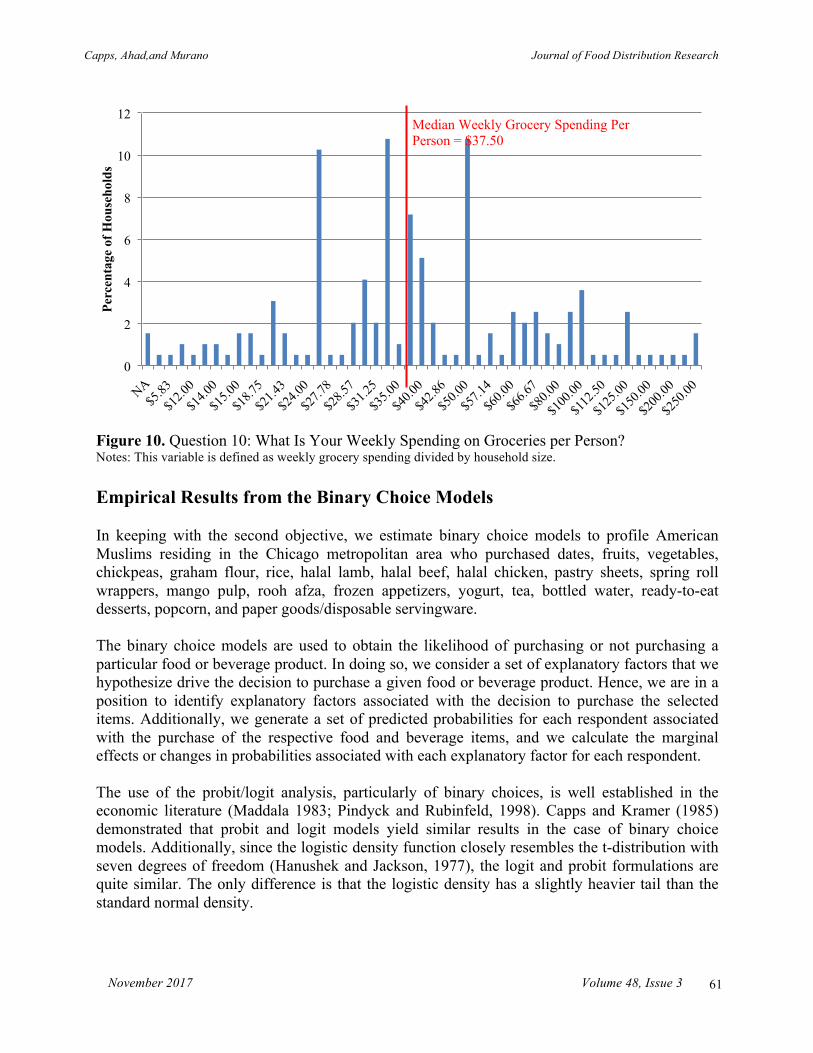
Capps, Ahad,and Murano Journal of Food Distribution Research
November 2017 Volume 48, Issue 3
61
Figure 10. Question 10: What Is Your Weekly Spending on Groceries per Person? Notes: This variable is defined as weekly grocery spending divided by household size. Empirical Results from the Binary Choice Models In keeping with the second objective, we estimate binary choice models to profile American Muslims residing in the Chicago metropolitan area who purchased dates, fruits, vegetables, chickpeas, graham flour, rice, halal lamb, halal beef, halal chicken, pastry sheets, spring roll wrappers, mango pulp, rooh afza, frozen appetizers, yogurt, tea, bottled water, ready-to-eat desserts, popcorn, and paper goods/disposable servingware. The binary choice models are used to obtain the likelihood of purchasing or not purchasing a particular food or beverage product. In doing so, we consider a set of explanatory factors that we hypothesize drive the decision to purchase a given food or beverage product. Hence, we are in a position to identify explanatory factors associated with the decision to purchase the selected items. Additionally, we generate a set of predicted probabilities for each respondent associated with the purchase of the respective food and beverage items, and we calculate the marginal effects or changes in probabilities associated with each explanatory factor for each respondent. The use of the probit/logit analysis, particularly of binary choices, is well established in the economic literature (Maddala 1983; Pindyck and Rubinfeld, 1998). Capps and Kramer (1985) demonstrated that probit and logit models yield similar results in the case of binary choice models. Additionally, since the logistic density function closely resembles the t-distribution with seven degrees of freedom (Hanushek and Jackson, 1977), the logit and probit formulations are quite similar. The only difference is that the logistic density has a slightly heavier tail than the standard normal density.
0
2
4
6
8
10
12 Pe
rcen
tage
of H
ouse
hold
s Median Weekly Grocery Spending Per Person = $37.50

Capps, Ahad,and Murano Journal of Food Distribution Research
November 2017 Volume 48, Issue 3
62
In this analysis, we fit both models (logit and probit) to the survey data. Additionally, we consider three functional forms associated with the logit/probit models: (1) the quadratic functional form (linear and quadratic terms for weekly grocery spending, household income, and household size as well as the interaction of household income and household size); (2) the linear functional form (only linear terms for the amount of weekly grocery spending, household income, and household size); and (3) the semi-logarithmic functional form (logarithmic transformations of the amount of weekly grocery spending, household income, and household size). These functional forms are not uncommon in the literature (e.g., Prais and Houthakker, 1955). The quadratic and semi-logarithmic functional forms are designed to capture potential non-linear relationships between the amount of weekly grocery spending, household income, and household size and the decision to purchase the various food and beverage items. Based on model selection criteria—namely AIC (Akaike Information Criterion), SIC (Schwarz Information Criterion), and HQC (Hannan-Quinn Criterion)—as well as log-likelihood and McFadden R2 statistics, we identified the appropriate functional form and binary choice model. For each food and beverage item the quadratic functional form was judged to be best based on the aforementioned criteria. For six of the food and beverage items (halal chicken, halal beef, bottled water, rice, ready-to-eat desserts, and yogurt) the logit model outperformed the probit model. For twelve of the food and beverage items (halal lamb, chickpeas, dates, frozen appetizers, graham flour, mango pulp, paper goods, pastry sheets, popcorn, rooh afza, spring roll wrappers, and tea), the probit model outperformed the logit model. Because roughly 98% of survey respondents reported purchasing fruits and vegetables, the lack of non-buyers with whom to compare buyers prohibited the estimation of the probit/logit models for these items. The probit model rests on the standard normal probability density function and the cumulative standard normal distribution function:
𝑓(𝑍!) =12𝜋
𝑒!!!!
!
(1) 𝑃! 𝑦! = 1 = 𝐹 𝑍! = 2𝜋 !!!!!!! 𝑒 − !! !
!𝑑𝑠
𝑍! = 𝑥!′𝛽
The logit model rests on the logistic probability density function and the cumulative logistic distribution function:
𝑓(𝑍!) = 𝑒!!/( 1+ 𝑒!! !) (2) P! y! = 1 = F Z! = e!!/(1+ e!!)
𝑍! = 𝑥!′𝛽 In the respective binary choice models, the dependent variable 𝑦! corresponds to the choice of purchasing or not purchasing any one of the aforementioned food and beverage products. Hence, 𝑦! can take only two values: 0 (for non-purchase) and 1 (for purchase). The index 𝑍! is a linear combination of all explanatory variables (𝑥!) in the model multiplied by their respective estimated coefficients.

Capps, Ahad,and Murano Journal of Food Distribution Research
November 2017 Volume 48, Issue 3
63
The explanatory variables considered in this analysis were: (1) the amount spent weekly in grocery stores; (2) the square of the amount spent weekly in grocery stores; (3) household size; (4) the square of household size; (5) the frequency of Ramadan hosting; (6) household income; (7) the square of household income; (8) the interaction of household income with household size; (9) ethnicity/race (included categories are South Asian, East Asian, European, and Middle Eastern/North African; the reference category was all other ethnicities/races); (10) the amount of additional spending during Ramadan; (11) openness to trying new food and beverage products; (12) whether dates were purchased during Ramadan (yes or no, included categories and California dates and Saudi dates; the reference category is other dates); (13) the purchase of halal beef (yes or no); (14) the purchase of halal chicken (yes or no) and (15) the purchase of halal lamb (yes or no). Because of missing entries from survey respondents for particular questions, the econometric analysis is conditional on 169 responses. The estimation of the logit/probit models rests on the use of maximum likelihood estimation. We use EVIEWS 8.0 as the software package to estimate the coefficients associated with the set of explanatory variables. Any estimated coefficient is deemed to be statistically different from zero provided the accompanying p-value is <0.10, the assumed level of significance in this study. Nearly all pairwise correlations among the explanatory variables from the quadratic functional form had an absolute value of <0.3. However, notable pairwise correlations were evident for weekly grocery spending and the square of weekly grocery spending (0.8964), household size \and the square of household size (0.9472), household income and the square of household income (0.9799), the interaction of household size and household income and household income (0.8449), and the interaction of household size and household income and the square of household income (0.8250). Belsley, Kuh, and Welsch (1980) point out that better diagnostics for collinearity among the explanatory variables include variance inflation factors (VIFs), condition indices, and variance decomposition proportions. On the basis of this information, no degrading collinearity (i.e., lack of redundant variables) was present. Hence, we are in a position to disentangle the impacts of the respective explanatory variables in the decision to purchase the food and beverage items included in the survey.3 Endogeneity may arise due to fact that the set of explanatory factors includes the decision to purchase chicken, lamb, and beef (respectively) in the binary choice models. We attempted to circumvent this issue by using instrument variables. Specifically, we replaced the actual values for the explanatory variables corresponding to the decision to purchase beef, chicken, and lamb (either 0 or 1) with predicted values based on first-stage estimates of all exogenous variables. That is, we estimated three additional binary choice models concerning the decision to purchase beef, chicken, and lamb as a function of all exogenous variables. The ensuing predicted values were probabilities that, by design, must be between 0 and 1. Essentially we used a two-stage estimation procedure in an attempt to combat potential endogeneity.4 3 We do not include the correlation matrix or the Belsley-Kuh-Welsh diagnostics due to space limitations. This information is available from the authors upon request. 4 Despite this effort, problems were evident with this procedure. First, the goodness-of-fit statistics associated with the first-stage binary choices models were not statistically different from zero. That is, the p-values of the chi-squared likelihood ratio statistics were 0.8497 (for

Capps, Ahad,and Murano Journal of Food Distribution Research
November 2017 Volume 48, Issue 3
64
Once the β coefficients are obtained via the use of maximum likelihood, estimates then are available for each index value, Zi=𝑥!!𝛽. Subsequently, once the index values are calculated, the probability of purchasing any food or beverage product is calculated for each respondent. The marginal effect for any explanatory variable is given by
(3) !!!!!!"
= 𝑓 𝑥!!𝛽 𝛽, where 𝑓(𝑥!!𝛽) is the probability density function for the respective binary choice model (see equations 1 and 2), 𝛽 corresponds to the set of estimated coefficients from the maximum likelihood procedure, i refers to the respondent in the sample, and xik refers to the value of the kth explanatory variable for the ith respondent. We assess the goodness-of-fit through the use of a chi-squared test and the McFadden R2 measure (McFadden, 1984). We also rely on prediction-success tables to validate the binary choice models. All of these metrics are standard in the evaluation of binary choice models (Pindyck and Rubinfeld, 1998). To formulate a prediction-success table, it is necessary to employ a decision rule for correct classifications of outcomes. Conventionally, if the predicted probability is ≤0.5, then the predicted outcome is Yi=0 (the respondent is predicted not to purchase). On the other hand, if the predicted probability is >0.5, then the predicted outcome is Yi=1 (the respondent is predicted to purchase). See Maddala (1983) and Pindyck and Rubinfeld (1998) to support this contention. However, Park and Capps (1997) point out that the appropriate cutoff may not necessarily be 0.5. Arguments have been made for the decision rule to be the ratio of the number of observations (respondent for which Yi=1) to the total number of observations. We adopt this decision rule in deriving the prediction-success table. Given space limitations, we report estimation results of the logit model for halal chicken in detail, including parameter estimates, standard errors, t-statistics, and p-values (Table 1). The logit/probit results for the remaining food and beverage items are available from the authors upon request.. The McFadden R2 metric is 0.5766, indicative of exceptional explanatory power of this binary choice model, especially since the data used in the econometric analysis are cross-sectional. The model explains a statistically significant amount of variation based on the likelihood ratio statistic of 49.94 with 17 degrees-of-freedom. The accompanying p-value of the likelihood ratio statistic, which follows a chi-squared distribution, is 0.000043.
halal chicken), 0.2187 (for halal beef), and 0.3769 (for halal lamb). Consequently, we were not able to identify any of the exogenous variables as instruments. Second, replacing the actual values for the explanatory variables that corresponded to the decision to purchase beef, chicken, and lamb (either 0 or 1) with predicted values based on first-stage estimates of all exogenous variables led to irreconcilable collinearity problems. Because of these problems, we believe the best course of action is to use the actual values for the explanatory variables (either 0 or 1) that correspond to the decision to purchase beef, chicken, and lamb. As such, we recognize the possibility of biased parameter estimates because of potential endogeneity.
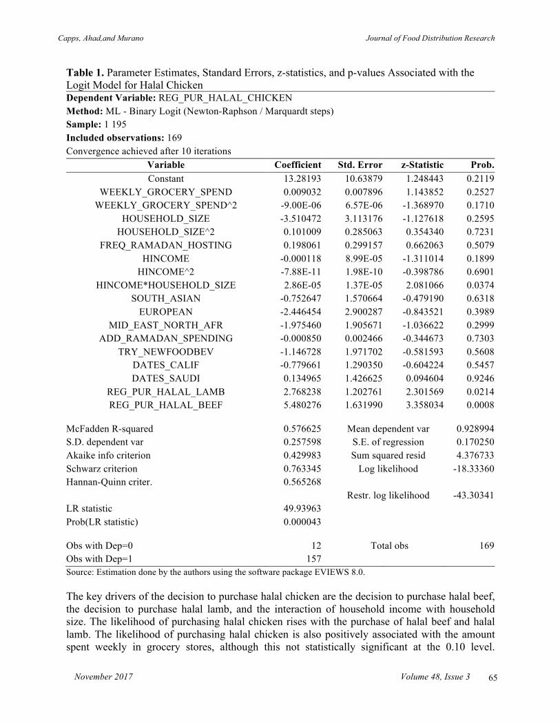
Capps, Ahad,and Murano Journal of Food Distribution Research
November 2017 Volume 48, Issue 3
65
Table 1. Parameter Estimates, Standard Errors, z-statistics, and p-values Associated with the Logit Model for Halal Chicken Dependent Variable: REG_PUR_HALAL_CHICKEN Method: ML - Binary Logit (Newton-Raphson / Marquardt steps) Sample: 1 195 Included observations: 169 Convergence achieved after 10 iterations
Variable Coefficient Std. Error z-Statistic Prob. Constant 13.28193 10.63879 1.248443 0.2119
WEEKLY_GROCERY_SPEND 0.009032 0.007896 1.143852 0.2527 WEEKLY_GROCERY_SPEND^2 -9.00E-06 6.57E-06 -1.368970 0.1710
HOUSEHOLD_SIZE -3.510472 3.113176 -1.127618 0.2595 HOUSEHOLD_SIZE^2 0.101009 0.285063 0.354340 0.7231
FREQ_RAMADAN_HOSTING 0.198061 0.299157 0.662063 0.5079 HINCOME -0.000118 8.99E-05 -1.311014 0.1899
HINCOME^2 -7.88E-11 1.98E-10 -0.398786 0.6901 HINCOME*HOUSEHOLD_SIZE 2.86E-05 1.37E-05 2.081066 0.0374
SOUTH_ASIAN -0.752647 1.570664 -0.479190 0.6318 EUROPEAN -2.446454 2.900287 -0.843521 0.3989
MID_EAST_NORTH_AFR -1.975460 1.905671 -1.036622 0.2999 ADD_RAMADAN_SPENDING -0.000850 0.002466 -0.344673 0.7303
TRY_NEWFOODBEV -1.146728 1.971702 -0.581593 0.5608 DATES_CALIF -0.779661 1.290350 -0.604224 0.5457 DATES_SAUDI 0.134965 1.426625 0.094604 0.9246
REG_PUR_HALAL_LAMB 2.768238 1.202761 2.301569 0.0214 REG_PUR_HALAL_BEEF 5.480276 1.631990 3.358034 0.0008
McFadden R-squared 0.576625 Mean dependent var 0.928994 S.D. dependent var 0.257598 S.E. of regression 0.170250 Akaike info criterion 0.429983 Sum squared resid 4.376733 Schwarz criterion 0.763345 Log likelihood -18.33360 Hannan-Quinn criter. 0.565268 Restr. log likelihood -43.30341 LR statistic 49.93963 Prob(LR statistic) 0.000043
Obs with Dep=0 12 Total obs 169 Obs with Dep=1 157 Source: Estimation done by the authors using the software package EVIEWS 8.0. The key drivers of the decision to purchase halal chicken are the decision to purchase halal beef, the decision to purchase halal lamb, and the interaction of household income with household size. The likelihood of purchasing halal chicken rises with the purchase of halal beef and halal lamb. The likelihood of purchasing halal chicken is also positively associated with the amount spent weekly in grocery stores, although this not statistically significant at the 0.10 level.

Capps, Ahad,and Murano Journal of Food Distribution Research
November 2017 Volume 48, Issue 3
66
Ethnicity/race, frequency of hosting during Ramadan, openness to trying new foods and beverages, and the decision to purchase dates during Ramadan are not statistically significant factors in the decision to purchase halal chicken. The marginal effects are calculated for each explanatory variable and for each respondent. We report the average of the marginal effects across respondents, highlighting the results for the statistically significant drivers of the decision to purchase halal chicken. The probability of purchasing halal chicken rises by 13.7 basis points if the decision is made to purchase halal lamb. The probability of purchasing halal chicken rises by 27.1 basis points if the decision is made to purchase halal beef. The probability of purchasing halal chicken rises by 3.5 basis points for every unit change in household size. The probability of purchasing halal chicken does not change appreciably due to changes in household income or to changes in the amount spent weekly in grocery stores. Based on the calculated marginal effects, the profile of any Muslim in the Chicago metropolitan area purchasing halal chicken rests primarily on their purchase of halal lamb or halal beef and household size . Nearly 93% of the survey respondents purchased halal chicken. Hence, in the derivation of the prediction-success table (Table 2), the cutoff probability for classification purposes is 0.93. That is, we predict that the ith respondent will purchase halal chicken if the probability of doing so exceeds 0.93. Within sample, the logit model correctly classifies the decision to not purchase halal chicken 11 out of 12 times, with 91.67% accuracy. Within sample, the logit model correctly classifies the decision to purchase halal chicken 140 out of 157 times, with 89.17% accuracy. Overall, within sample, the model correctly classifies all decisions 151 out of 169 times, with 89.35% accuracy. Thus, we validate that the logit model does extremely well in correctly classifying the decision to purchase halal chicken and the decision not to purchase halal chicken. Table 2. Prediction-Success Outcomes for the Decision to Purchase Halal Chicken Actual y=1 Actual y=0 Predicted y=1 140 1 Predicted y=0 17 11
Source: Calculations by the authors. Given space limitations, Table 3 summarizes the logit/probit results for the remaining food and beverage items from this survey. Significant coefficients associated with the respective set of explanatory factors are listed along with +/- signs of the estimated coefficients. Key determinants concerning the decision to purchase the remaining food and beverage items were as follows:5 Purchase of halal beef was a driver of the decision to purchase halal lamb, graham flour, mango pulp, paper goods, pastry sheets, popcorn, rice, rooh afza, spring roll wrappers, and tea. Purchase of halal lamb was a driver of the decision to purchase mango pulp, rice, ready-to-eat desserts, and yogurt. Purchase of halal chicken was a determinant of the decision to purchase halal beef and halal lamb. The amount spent weekly in grocery stores influenced the decision to purchase halal beef, bottled water, paper goods, pastry sheets, rice, tea, and yogurt. Household size was a driver in the decision to purchase halal beef, dates, rooh afza, and yogurt. Household income was a determinant of the decision to purchase halal beef, chickpeas, graham flour, pastry sheets, rice, 5 Recall that it was not possible to estimate binary choice models for fruit and vegetables . Virtually the entire sample from the Chicago metropolitan area purchased these items.
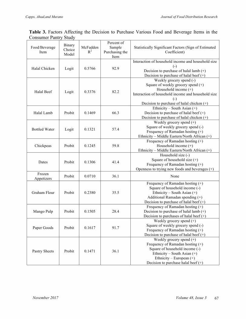
Capps, Ahad,and Murano Journal of Food Distribution Research
November 2017 Volume 48, Issue 3
67
Table 3. Factors Affecting the Decision to Purchase Various Food and Beverage Items in the Consumer Pantry Study
Food/Beverage Item
Binary Choice Model
McFadden R2
Percent of Sample
Purchasing the Item
Statistically Significant Factors (Sign of Estimated Coefficient)
Halal Chicken Logit 0.5766 92.9
Interaction of household income and household size (-)
Decision to purchase of halal lamb (+) Decision to purchase of halal beef (+)
Halal Beef Logit 0.3376 82.2
Weekly grocery spend (-) Square of weekly grocery spend (+)
Household income (+) Interaction of household income and household size
(-) Decision to purchase of halal chicken (+)
Halal Lamb Probit 0.1469 66.3 Ethnicity – South Asian (+)
Decision to purchase of halal beef (+) Decision to purchase of halal chicken (+)
Bottled Water Logit 0.1321 57.4
Weekly grocery spend (+) Square of weekly grocery spend (-) Frequency of Ramadan hosting (+)
Ethnicity – Middle Eastern/North African (+)
Chickpeas Probit 0.1245 59.8 Frequency of Ramadan hosting (+)
Household income (+) Ethnicity – Middle Eastern/North African (+)
Dates Probit 0.1306 41.4
Household size (-) Square of household size (+)
Frequency of Ramadan hosting (+) Openness to trying new foods and beverages (+)
Frozen Appetizers Probit 0.0710 36.1 None
Graham Flour Probit 0.2380 35.5
Frequency of Ramadan hosting (+) Square of household income (-)
Ethnicity – South Asian (+) Additional Ramadan spending (+)
Decision to purchase of halal beef (+)
Mango Pulp Probit 0.1505 28.4 Frequency of Ramadan hosting (+)
Decision to purchase of halal lamb (+) Decision to purchases of halal beef (+)
Paper Goods Probit 0.1617 91.7
Weekly grocery spend (+) Square of weekly grocery spend (-) Frequency of Ramadan hosting (+)
Decision to purchase of halal beef (+)
Pastry Sheets Probit 0.1471 36.1
Weekly grocery spend (+) Frequency of Ramadan hosting (+)
Square of household income (-) Ethnicity – South Asian (+)
Ethnicity – European (+) Decision to purchase halal beef (+)

Capps, Ahad,and Murano Journal of Food Distribution Research
November 2017 Volume 48, Issue 3
68
Popcorn Probit 0.1808 53.8
Ethnicity – East Asian (+) Openness to trying new foods and beverages (+)
Decision to purchase California dates during Ramadan (-)
Decision to purchase Saudi dates during Ramadan (-)
Decision to purchase of halal beef (+)
Rice Logit 0.3755 92.9
Weekly grocery spend (-) Square of weekly grocery spend (+)
Household income (+) Square of household income (-)
Decision to purchase California dates during Ramadan (-)
Decision to purchase of halal beef (+) Decision to purchase of halal lamb (+)
Rooh Afza Probit 0.1907 14.2 Square of household size (-) Decision to purchase of halal beef (+)
Ready-to-eat-Desserts Logit 0.0819 46.2
Decision to purchase California dates during Ramadan (-)
Decision to purchase Saudi dates during Ramadan (-)
Decision to purchase of halal lamb (+)
Spring Roll Wrappers Probit 0.1492 25.4
Frequency of Ramadan hosting (+) Square of household income (-)
Ethnicity – South Asian (+) Ethnicity – Middle Eastern/North African (+)
Decision to purchase of halal beef (+)
Tea Probit 0.1629 84.6
Weekly grocery spend (-) Square of weekly grocery spend (+)
Household size (+) Decision to purchase of halal beef (+)
Yogurt Logit 0.2509 87.6
Weekly grocery spend (-) Household size (+)
Ethnicity – South Asian (+) Additional Ramadan spending (+)
Decision to purchase of halal lamb (+)
Capps, Ahad,and Murano Journal of Food Distribution Research
November 2017 Volume 48, Issue 3
69
and spring roll wrappers. Ethnicity was important in the decision to purchase halal lamb, bottled water, chickpeas, graham flour, pastry sheets, popcorn, spring roll wrappers, and yogurt. Frequency of hosting Ramadan was a factor in the decision to purchase bottled water, chickpeas, dates, graham flour, mango pulp, paper goods, pastry sheets, and spring roll wrappers. Openness to trying new foods and beverages was a driver of the decision to purchase dates and popcorn, while additional spending for Ramadan was a driver of the decision to purchase graham flour and yogurt. Moreover, purchase of dates during Ramadan was important in the decision to purchase popcorn, rice, and ready-to-eat desserts. No explanatory factors influenced the decision to purchase frozen appetizers. Concluding Remarks Although the literature concerning Muslim consumers and halal food purchasing behavior is limited, previous studies have identified several behavioral predictors—including consumer confidence, intention, and perceived behavior control—and subjective norms. Several studies have focused on the international community of Muslims, and one study described consumer purchase behavior of halal products produced by non-Muslim manufacturers. Our study builds on this foundation by investigating sociodemographic factors and habits related to purchases of specific halal food and beverage products by American Muslim consumers residing in the northern suburbs of Chicago. A majority of respondents in our survey spent more on groceries during Ramadan than in other months; we also observed statistical significance for multiple explanatory factors regarding the decision to purchase the food and beverage items in this study. The chief drivers, in terms of the number of statistically significant coefficients, in the decision to purchase the respective food and beverage items were the purchase of halal beef, the amount spent weekly in grocery stores, the frequency of hosting Ramadan, household income, household size, and ethnicity (in that order). The purchase of halal chicken, openness to trying new foods and beverages, additional grocery spending during Ramadan, and the purchase of dates during Ramadan were influencers for only two or three of the food and beverage items studied. This study helps ascertain the buying preferences of American Muslims at least for a particular geographical area. Our study was limited in scope, being restricted to one urban geographical location, yet it provides a snapshot of purchasing behavior in a segment of American Muslim consumers. In subsequent research efforts, the methodology should be replicated in other regions to broaden the dataset and achieve greater representation of this population. This pilot study provides a baseline for spending habits and buying preferences for twenty food and beverage items which had been lacking in the extant literature. Given the rise in interest in and the growing importance of the Muslim community in the United States, this information is of value to stakeholders in the U.S. food industry supply chain. Developing business potential in the halal food industry worldwide is currently receiving much attention. Consequently, applications of the results from our research may provide strategic opportunities for stakeholders in the food industry who are poised to meet the demands of the American Muslim community.
Capps, Ahad,and Murano Journal of Food Distribution Research
November 2017 Volume 48, Issue 3
70
Acknowledgments This research was funded by the Islamic Food and Nutrition Council of America. References Alam, S.S, and N.M. Sayuti. 2011. “Applying the Theory of Planned Behavior (TPB) in
Halal Food Purchasing.” International Journal of Commerce and Management 21(1), 8–20.
American Muslim Consumer Consortium. 2015. “American Muslim Consumer Market Study – Session I.” AMCC 2014 meeting, Newark NJ, 15 November. Available online: http://2014.americanmuslimconsumer.com/
Belsley, D., E. Kuh, and R. Welsch, 1980. Regression Diagnostics: Identifying Influential Data and Sources of Collinearity. New York: Wiley.
Capps Jr., O., and R.A. Kramer. 1985. “Analysis of Food Stamp Participation Using Qualitative Choice Models.” American Journal of Agricultural Economics 67(1): 49–59.
Dinar Standard. 2015. “The Muslim Green: American Muslim Market Study 2014/15.” New York. Available online: http://www.dinarstandard.com/american-market-2014/
EVIEWS. Available online: http://www.eviews.com
Golnaz, R., M. Zainalabidin, S. Mad Nasir, and F.C. Eddie Chiew. 2010. “Non-Muslims’ Awareness of Halal Principles and Related Food Products in Malaysia.” International Food Research Journal 17: 667–674.
Hanushek, J., and E. Jackson. 1977. Statistical Methods for Social Scientists. New York: Academic Press.
Irfan, M. 2014. “Muslim Buying Power.” Muslim Observer. Available online: http://muslimobserver.com/muslim-buying-power-new-consumer-survey-highlights-muslim-american-spending-power-increased-demand-for-ethical-islamic-goods/
Islamic Food and Nutrition Council of America. Available online: http://www.ifanca.org/
Maddala, G.S. 1983. Limited Dependent and Qualitative Variables in Econometrics. Cambridge: Cambridge University Press.
McFadden, D. 1984. “Econometric Analysis of Qualitative Response Models.” in Z. Griliches and M. Intriligator, eds., Handbook of Econometrics, Volume 2, Amsterdam: North Holland, pp. 1395–1457.

Capps, Ahad,and Murano Journal of Food Distribution Research
November 2017 Volume 48, Issue 3
71
Mohamed, B. 2016. “A New Estimate of the U.S. Muslim Population.” Pew Research Center. Available online: http://pewrsr.ch/1PfaUs5
Omar, K.M, NK.N. Mat, G.A. Imhemed, F.M.A. Ali. 2012. “The Direct Effects of Halal Product Actual Purchase Antecedents among the International Muslim Consumers.” American Journal of Economics Special Issue: 87–92.
Park, J.L., and O. Capps Jr. 1997. “The Demand for Prepared Meals by U.S. Households.” American Journal of Agricultural Economics 79(3): 814–824.
Pindyck, R.S., and D. L. Rubinfeld. 1998. Econometric Models and Economic Forecasts, 4th ed. New York: McGraw-Hill.
Prais, S.J., and H.S. Houthakker. 1955. The Analysis of Family Budgets. Cambridge: Cambridge University Press.
U.S. Census Bureau. 2017. Advance Monthly Retail Trade Report. Washington, DC: U.S. Census Bureau, October 13. Available online: https://www.census.gov/retail/index.html
Yunus, N.S.N.M., W.E.W. Rashid, N.M. Ariffin, and N. M. Rahid. 2014. “Muslim's Purchase Intention towards Non-Muslim's Halal Foods Packaged by Food Manufacturers,” Procedia - Social and Behavioral Sciences 130:145–154.
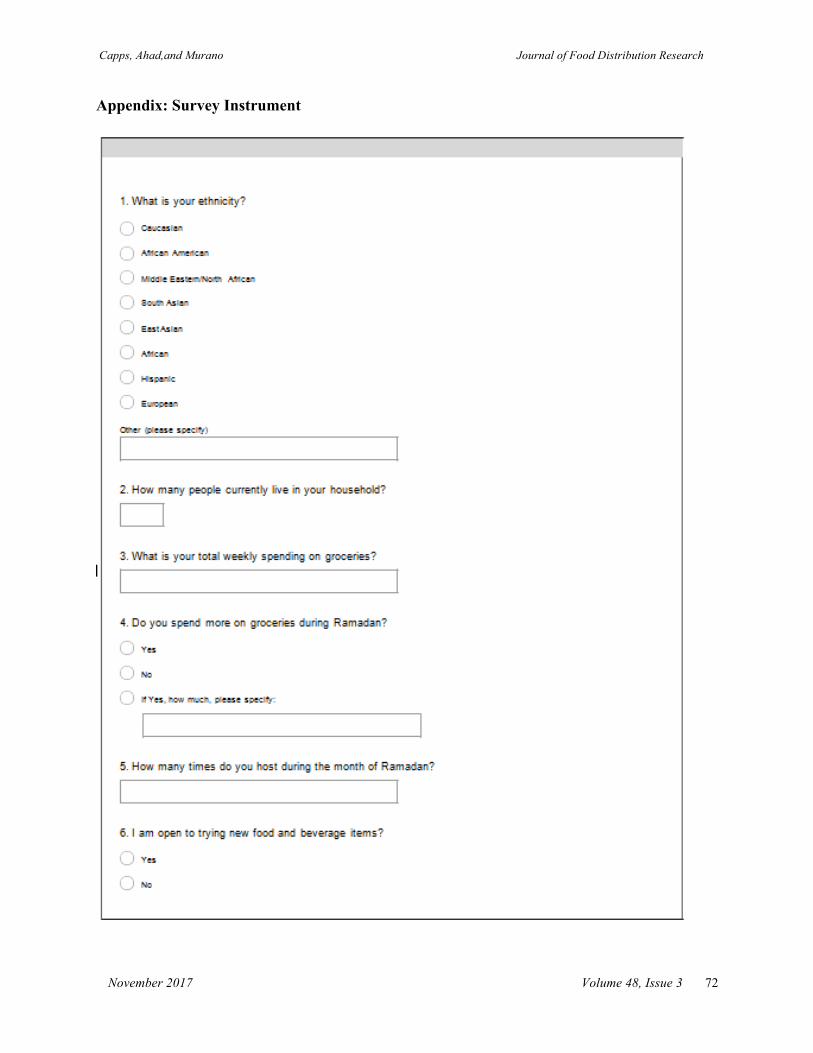
Capps, Ahad,and Murano Journal of Food Distribution Research
November 2017 Volume 48, Issue 3
72
Appendix: Survey Instrument

Capps, Ahad,and Murano Journal of Food Distribution Research
November 2017 Volume 48, Issue 3
73
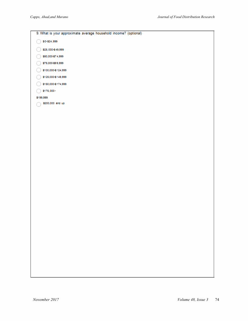
Capps, Ahad,and Murano Journal of Food Distribution Research
November 2017 Volume 48, Issue 3
74