VOLTAGE STABILITY ANALYSIS OF POWER

SYSTEMS USING THE CONTINUATION METHOD

Code: 19.003

A. D. Vasquez, T. Sousa

Federal University of ABC, Brasil

1

1. Objectives

2. Introduction

3. The Voltage Stability

5. The Continuation Power Flow

6. Voltage Stability Margin (VSM)

7. Tests and Results

8. Discussion

9. Conclusions

Summary

2

Inclusion of renewable energy sources in the system.

Impacts in the normal functioning of electric grids, caused by the

integration of intermittent sources in the system.

Voltage stability researching based in the determination of the

maximum loading of the electrical power system.

Application of the continuation method to the power flow problem

to improve the simulations performance.

Computing the algorithm by parallel programation techniques to

decrease the simulation time.

Objectives

3

GROWING PLANNING AND VOLTAGE

DEMAND OPERATION SECURITY

TRANSFER OF LARGE

AMOUNTS OF POWER OPERATION IN CONTINUATION

STRESSFUL POWER FLOW

ECONOMIC AND CONDITIONS (CPF)

ENVIRONMENTAL P-V Curve drawing and

REQUIREMENTS computation of the system

Maximum Loading Point (MLP)

- Voltage stability margin and modal analysis studies;

- Determining effective measurements for strengthening the system;

- Analysis of static phenomenon such as the voltage stability.

Introduction

4

Ability of a power system to maintain acceptable 𝑉𝑖 (𝑖 = 1,… ,𝑁𝐵) under

normal conditions and after being subjected to a disturbance.

Disturbances

CAUSED BY Increase in load demand

Change in system condition

There is a need for analytical tools capable of:

Predicting voltage collapse in complex networks;

Accurately quantifying stability margins and power transfer limits;

Identifying voltage-weak points and areas susceptible to voltage

instability;

Identifying key contribution factors and sensitivities that provide insight

into system characteristics to assist in developing remedial actions.

The Voltage Stability

5

Captures “snapshots” of system conditions at various

time frames along the time-domain trajectory

Static analysis of voltage stability involves the static model

of the power system and it is based on the modal analysis

of the power flow Jacobian matrix, as shown in (1)

∆𝑃𝑃𝑄,𝑃𝑉∆𝑄𝑃𝑄

=𝐽𝑃𝜃 𝐽𝑃𝑉𝐽𝑄𝜃 𝐽𝑄𝑉

∙∆𝜃∆𝑉𝑃𝑄

(1)

A. Static Analysis

6

This theory is used to describe changes in the qualitative structures of the

phase portrait when certain system parameters change.

SADDLE-NODE BIFURCATION Point of voltage collapse

A saddle-node bifurcation is the disappearance of a

system equilibrium as parameters change slowly.

The saddle-node bifurcation occurs when a stable

equilibrium at which the power system operates disappears.

𝑓 𝑥, 𝜆 = 𝑥 = 𝜆 − 𝑥2 (2)

system state

system parameter

B. Bifurcation Theory

7

Using the continuation method, a solution branch

around the turning point can be tracked without

difficulties. The CPF captures the path-following

feature by means of a predictor-corrector scheme

that adopts locally parameterized continuation

techniques to trace the Power Flow solution paths. Adapted from [7].

Reformulation of Power Flow (PF) Equations

The PF equations are reformulated including a

load parameter λ.

Δ𝑃𝑖 = 𝑃𝐺𝑖 𝜆 − 𝑃𝐿𝑖 𝜆 − 𝑃𝑇𝑖 = 0 (3)

Δ𝑄𝑖 = 𝑄𝐺𝑖 𝜆 − 𝑄𝐿𝑖 𝜆 − 𝑄𝑇𝑖 = 0 (4)

The Continuation Power Flow

8

Fig. 1. Predictor-corrector scheme used in the CPF.

The entire set of

equations is

denoted as 𝐹 and

the problem can be

expressed as (5). 𝐹 𝛿, 𝑉, 𝜆 = 0 0 𝑜𝑢 𝟏 ≤ 𝜆 ≤ 𝜆𝑐𝑟𝑖𝑡𝑖𝑐𝑎𝑙 (5)

𝑭𝜹 𝑭𝑽 𝑭𝝀

𝒅𝜹𝒅𝑽𝒅𝝀

= 𝟎 (6)

If the index 𝑘 represents the continuation parameter position and it is

chosen properly, the tangent vector is determined as the solution by (7).

𝑭𝜹 𝑭𝑽 𝑭𝝀

𝒆𝒌𝒕 =

𝟎𝒕𝒌

, 𝒕𝒌 = ±𝟏 (7)

𝜹𝒑

𝑽𝒑

𝝀𝒑 𝒋+𝟏

=𝜹𝑽𝝀 𝒋

+ 𝝈𝒋

𝒅𝜹𝒅𝑽𝒅𝝀

(8)

𝝈𝒋 𝒏𝒆𝒘=

𝝈𝒋 𝒐𝒍𝒅

𝒕 (9)

A. Prediction Step

9

Tangent predictor technique

Predicted Solution

Step Size

The original set of equations is

augmented by one equation that

specifies the value of one of the state

variables. The 𝑘𝑡ℎ element has a

proper value considering that 𝑥𝑘 = 𝜂

and the new set of equations will be

as follows in (10).

𝐹(𝑥)𝑥𝑘 − 𝜂

= 0 (10)

Once the original equations system is

altered by an additional equation and

one additional state variable is

involved, a corrector method (NR) is

used to solve the system.

B. Local Parameterization

and Corrector Step

10

C. The Critical Bus

Identification

P and Q transmission is very close

to the limit value.

The voltage control actions in a

critical bus may have opposite

consequences than expected

More sensitive due to

disturbances in the power system.

Mathematically, using the tangent

vector method, the critical bus will be

denoted by the index 𝑐 and will be

obtained by (11).

𝑐 ← 𝑚𝑎𝑥𝜕𝑉1

𝜕𝜆,𝜕𝑉2

𝜕𝜆, …

𝜕𝑉𝑛

𝜕𝜆 (11)

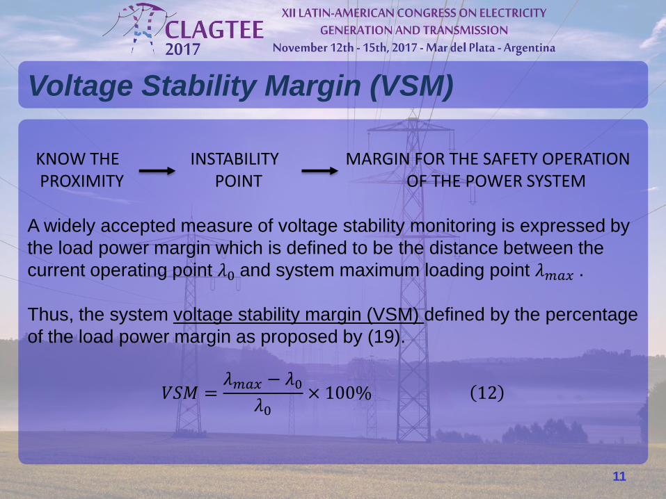
KNOW THE INSTABILITY MARGIN FOR THE SAFETY OPERATION PROXIMITY POINT OF THE POWER SYSTEM A widely accepted measure of voltage stability monitoring is expressed by

the load power margin which is defined to be the distance between the

current operating point 𝜆0 and system maximum loading point 𝜆𝑚𝑎𝑥 .

Thus, the system voltage stability margin (VSM) defined by the percentage

of the load power margin as proposed by (19).

𝑉𝑆𝑀 =𝜆𝑚𝑎𝑥 − 𝜆0

𝜆0× 100% 12

Voltage Stability Margin (VSM)

11

IEEE-57-bus Test System

Fig. 2. Diagram for the IEEE 57-bus test system.

Test and Results

12

1 1.05 1.1 1.15 1.2 1.250.8

0.82

0.84

0.86

0.88

0.9

0.92

0.94

0.96

0.98

1

Load ()

Vo

ltag

e m

ag

nitu

de

[p

u]

PV Curve

Critical bus: Bus31

7 Generators

15 LTCs 65 transmission elements

42 loads

Fig. 3. Voltage Profile in the critical bus for original IEEE 57-bus test system.

VSM= 17.68%

Case 1: Distributed Generator (DG) in B-31

For the first test case, a large generator with

50 [MW] and 30 [MVAr] in the original critical

bus of the system is incorporated.

Fig. 4. Voltage Profile in the critical bus for Case 1.

Critical Bus: 25

VSM= 28.68%

13

Case 2: DG in a High Load Area

In the northeast area of the system is

concentrated the 48.24% of the active load

and 26.53% of the reactive For this reason,

the same DG is allocated in the B-37.

Fig. 5. Voltage Profile in the critical bus for Case 2.

Critical Bus: 31

VSM= 28.16%

1 1.05 1.1 1.15 1.2 1.25 1.3 1.35 1.41.06

1.07

1.08

1.09

1.1

1.11

1.12

Load ()

Vo

ltag

e m

ag

nitu

de

[pu

]

PV Curve

Critical bus: Bus25

1 1.05 1.1 1.15 1.2 1.25 1.3 1.35 1.40.93

0.94

0.95

0.96

0.97

0.98

0.99

1

Load ()

Vo

ltag

e m

ag

nitu

de

[pu

]

PV Curve

Critical bus: Bus31

Case 3: DG in a distant bus from the original

generation: A bus is selected in the middle

of the mesh transmission network. Thus, for

guarantee its similar distance with all the

generators located in the original system:

Bus 36.

Fig. 6. Voltage Profile in the critical bus for Case 3.

Critical Bus: 31

VSM= 28.70%

14

Case 4: 2 DG’s connected in strategic buses

The additional generation for the system is

included using two identical distributed

generators. Each of them injects 25 [MW]

and 15 [MVAr] to the system and are

allocated in buses 36 and 37.

Fig. 7. Voltage Profile in the critical bus for Case 4.

Critical Bus: 31

VSM= 35.93%

1 1.05 1.1 1.15 1.2 1.25 1.3 1.35 1.40.96

0.97

0.98

0.99

1

1.01

1.02

Load ()

Vo

ltag

e m

ag

nitu

de

[p

u]

PV Curve

Critical bus: Bus31

1 1.05 1.1 1.15 1.2 1.25 1.3 1.35 1.4 1.45

0.97

0.98

0.99

1

1.01

1.02

Load ()

Vo

ltag

e m

ag

nitu

de

[p

u]

PV Curve

Critical bus: Bus31

The Case 4 obtains the best stability scenario where the VSM has the

greatest value, increasing from 17.68% in the original case to 35.93% and

the final magnitude voltage in the critical bus (bus 31) is 0.98 [pu].

This results shows injection of distributed generation in strategic points of

the system affects directly the voltage stability margin and the voltage

profile of the buses in the system.

Based in this information, it is possible to affirm that is better divide the

power injection in a mesh system than concentrate the distributed

generation just in a strategic bus. Thus, using different criteria for selecting

strategic connection points in the system and installing the same total

additional power distributed in these points, the voltage stability improves

considerably.

Discussion

15

The CPF methodology is considering a computational simulation tool to

aid in operating, planning and investment decisions in power systems.

The injection of active power and compensation of reactive power in

the system was studied using different allocations for the same

apparent power.

The best criteria to include distributed generation in the system is

selecting more than one injection point in different areas of the system

and divide the total apparent power in these connection points.

The simulation time for this system using parallel programation

techniques corresponds to 2.66 milliseconds.

The future work consists in improving this time, including a Graphic

Processing Unit in the methodology to process the information in large

transmission and distribution systems.

Conclusions

16

17

Thank you !