Volatility Regime-Switching and Linkage among GCC … · volatility regimes. Correlations of the...
22
1 Paper Prepared for the 11 th ERF Conference on December 16-18, 2004 Volatility Regime-Switching and Linkage among GCC Stock Markets Shawkat Hammoudeh Drexel University Philadelphia, PA Kyongwook Choi Ohio University Athens, OH Abstract. The GCC stock markets vary in terms of sensitivity to the magnitude of return volatility and the duration of volatility, regardless of the volatility regime and the return component. Among the GCC market, risk-averse investors and traders in the Oman and Saudi Arabia markets should particularly demand higher premiums for the extra volatility sensitivity during fad times than investors in the other markets. In terms of duration of volatility, investors and policy makers in the Kuwait, Bahrain and Saudi Arabia should be aware of the longer duration of this volatility during the fad times. All GCC returns move in the same direction whether in terms of total return, fundamentals or fads under both volatility regimes. Correlations of the stock returns and their components with each other and with the oil price return are also weak, suggesting that country particularities in addition to the oil price return influence the stock component returns. JEL Classification: C22; F3; Q49 Keywords : Volatility; Markov switching; Permanent and transitory components; Transition Probability
Transcript of Volatility Regime-Switching and Linkage among GCC … · volatility regimes. Correlations of the...

1
Paper Prepared for the 11th ERF Conference on December 16-18, 2004
Volatility Regime-Switching and Linkage among GCC Stock Markets
Shawkat Hammoudeh Drexel University Philadelphia, PA
Kyongwook Choi Ohio University
Athens, OH
Abstract. The GCC stock markets vary in terms of sensitivity to the magnitude of return
volatility and the duration of volatility, regardless of the volatility regime and the return
component. Among the GCC market, risk-averse investors and traders in the Oman and
Saudi Arabia markets should particularly demand higher premiums for the extra volatility
sensitivity during fad times than investors in the other markets. In terms of duration of
volatility, investors and policy makers in the Kuwait, Bahrain and Saudi Arabia should be
aware of the longer duration of this volatility during the fad times. All GCC returns move
in the same direction whether in terms of total return, fundamentals or fads under both
volatility regimes. Correlations of the stock returns and their components with each other
and with the oil price return are also weak, suggesting that country particularities in
addition to the oil price return influence the stock component returns.
JEL Classification: C22; F3; Q49 Keywords: Volatility; Markov switching; Permanent and transitory components; Transition Probability

2
Volatility Regime-Switching and Linkage among GCC Stock Markets
1. Introduction
Fads or speculative attacks are short- lived phenomena that affect the world’s
stock markets such as the October 1997 crash of the US market and the 1982 crash of the
Kuwait market. In these crashes the markets experience large drop in stock prices and
dramatic jump in volatility. Shocks in the fads are caused by noisy trades how bid prices
away from the fundamentals due to changes in price misperceptions (De Long et al,
1990). Although the fad volatility usually reverts to normal levels quickly, this transitory
volatility can cause tremendous damage to wealth and social wellbeing. Moreover,
increases in risk would raise the cost of capital and may retard economic growth in the
long-run. Therefore, it is important to consider an economic variable such as a stock
return in terms of its permanent or fundamental component, and its transitory or fad
components to determine the expected durability of the fad volatility relative to the
fundamental volatility and examine the impact of each of these components on the
volatility of the return.
The recent literature also studies the decomposition of the stock return within the
state-space framework that allows for volatility transition between regimes for the return
itself and for each of its components. Several authors have proposed different methods of
decomposing a time series into permanent and transitory components. Nelson and Plosser
(1982) matched a model consisting of transitory and permanent components to an
autocorrelation function to determine the relative sizes of these two components. Watson

3
(1986) and Clark (1987) used the conventional unobserved component model (without
Markov-switching) to decompose GNP into these two components. Campbell and
Mankiw (1987), employing an ARMA representation of a time series, estimated the
impact of a shock on long-run forecasts to weigh up he relative importance of the two
components.
More recent methods examined the decomposition by focusing on mean reversion
in stock returns. Fama and French (1988) used an autoregressive test and found mixed
results on the existence of mean reversion in the transitory and permanent components.
Kim and Kim (1996) and Kim and Nelson (1999) examined the relative importance of the
two components within the framework of the space state model with Markov-switching
heteroscedasticity. This model can capture the short term dynamics that might not
otherwise be captured by the other methods such as the autoregression test of Fama and
French (1988) and the conventional unobserved component models of Watson (1986) and
Clark (1987). Bhar and Hamori (2004) applied Kim and Kim (1996) model to the some
of OECD countries. Other studies that use the space-state model with a Markov regime-
switching process to model volatility and shifts in return regimes but without the
component decomposition include Hamilton and Susman (1994)1, McCarthy and Najand
(1995), Chu et al (1996), Schaller and van Norden (1997) and among others.
This study uses the empirical model of Kim and Kim (1996) and Bhar and
Hamori (2004) to examine the volatility of the decomposed stock returns of members of
the Gulf Cooperation Council (GCC). The six-member GCC includes: Bahrain, Kuwait,
1 For earlier research, see Hamilton (1989), Turner et al (1989) and Glosten et al (1993).

4
Oman, Qatar, Saudi Arabia and United Arab Emirates (UAE)2. The market capitalization
of the GCC markets as a group was about US$ 172 billion at the end of 2002, and since
then has been rapidly rising because of high oil prices and of strong movement towards
privatization. These markets have strong future gain potential because of their ownership
of huge oil reserves. They together account for 16% of the world output and possess 47%
of the world’s oil reserves. In 2002 when most of the world’s stock markets dropped
drastically and realized huge losses, most of the GCC countries made substantial gains
and have continued this strong gain through 2004.
Recent research on the GCC stock markets uses the error-correction model to
examine co-movements and interactions of the returns (Hammoudeh and Eleisa, 2004;
and Malik and Hammoudeh, 2004). No attempt has been made to examine the mean
reversion of the two components that make up the returns of these GCC markets while
allowing for volatility regime switching. Therefore, the desired objectives of this paper
can be summarized as follows:
1. To decompose the stock returns of the GCC stock markets into permanent and
transitory components;
2. To measure the switch in volatility between the high and low variance regimes for
both the permanent and transitory components of the stock returns;
3. To measure the expected duration of the volatility, in terms of trading weeks, of
the high and low variance regimes of the transitory component.
2 Qatar is not included because its stock market was established in 1997, which does not provide an appropriate long enough time series.

5
4. To measure the correlation between the volatilities of the individual GCC stock
markets to ascertain whether or not these markets move in the same or opposite
direction; and
5. To measure the correlation of volatility of the individual GCC stock markets and
oil markets to determine if they move in the same direction.
The findings suggest that there are two significant volatility-switching regimes in
both components of the stock returns for all the GCC countries. They also show
differences in the sensitivity to the return volatility and the duration of volatility across
regimes and return components and across the markets. In particular the results
emphasize the sensitivity of the Oman and Saud i markets to shocks during fad times in
the high volatility regime which is of particular interest to this study. Shocks also persist
longer in the Kuwait, Bahrain and Oman markets in the high volatility fad regime. We
should also note that shocks in the fundamentals have very long expected durations
exceeding the durations of shocks in the fads. Overall, these results suggest that the GCC
countries are very different when it comes to return on financial investment. Thus,
investors should do their homework before investing in these countries. Moreover, the
persistence and magnitude of extra volatility in certain markets (e.g., Oman and Kuwait)
calls on policy makers to introduce financial hedge instruments (e.g., options, futures) to
help investors ride the volatility waves that could persist for several months. They should
reduce volatility because of its impact on the cost of capital and economic growth.
Traders should also demand higher premiums for investing in stock markets that are
relatively more volatile such as the Oman market. The findings will provide traders and

6
investors in the GCC markets with information that may enable them to distinguish
between markets and ask for higher compensations in some markets than others.
The results also indicate that the markets are not highly correlated in the return itself,
and the permanent and transitory components between the GCC markets, compared for
example with Germany, Japan, UK and the United States (Bhar and Hamori, 2004).
These results suggest there are some gains from portfolio diversification among particular
GCC markets particula rly between Saudi Arabia and UAE, and between and Oman and
Bahrain.
The correlations of the returns and their components with the oil price for the
countries are also weak, suggesting that country particularities also influence the
component returns. The weakest correlation is between the oil price return and the Oman
and Kuwait total returns. The Kuwait market has a negative correlation with the oil price
return in the fads, emphasizing the importance of speculative attacks and the presence of
hot hands in this market. This information is useful for local as well as for international
investors
2. Descriptive Statistics
The Gulf Cooperation Council (GCC) consists of six members including Bahrain,
Kuwait, Oman, Qatar, Saudi Arabia and United Arab Emirates. We used in this study
weekly time series on the Bahrain Stock Exchange index (BSE), Kuwait Stock Exchange
index (KSE), the Oman Muscat Securities Market index (MSM), the Saudi stock market
index (Tadawal) and the UAE National Bank of Abu Dhabi index (NBAD). As indicated
above, the market capitalization of the GCC markets as a group was about US$ 172

7
billion at the end of 2002. These stock markets display low to moderate valuations
compared to the stock markets in the United States and other major world markets
(Hammoudeh and Eleisa, 2004)
The series for these indices were directly obtained from the respective stock
exchanges. The data for these series covers the period February 15, 1994 to December
25, 2001. The sample period was determined primarily by the availability of the data on
the five Gulf equity markets. Still, this sample period includes the Mexican 1994 crisis,
the July 1997 East Asian crisis, the 1998 collapse of oil prices, the 1999 oil price and
Asian economy recovery, the adoption of the target zone oil pricing mechanism in
February 2000, and the New York September 2001 bombing. The rate of return on for
each country’s each stock index is calculated as a log-differenced
prices, 1(log( ) log( )) 100t t tr P P −= − × , where tP is the stock price index for each country.
Comparing the volatilities of the five GCC stock indices and the Dow as defined
by the coefficient of variation, Table 1 shows that the GCC stock returns on average are
less volatile than the DOW which could be due to the isolation of these markets and the
difference in the types of traders participating in them; the only exception is the Omani
index (MSM) which is the most volatile of them all. It also shows that the six stock
returns are generally more volatile than the five spot and futures oil price returns.
However, the US DOW return is highly skewed to the left, while the GCC returns are
moderately skewed to the right. This means that there is a higher probability for investors
to get positive returns from the GCC markets rather than negative returns, as is the case
in developed and some other emerging markets (Harvey and Siddique, 1999). An
expectation of positive rather than negative returns in a portfolio of oil-sensitive GCC
8
stocks is a manifestation of anticipated higher compensation for the higher risk associated
with a narrowly diversified portfolio.
A stylized fact of individual financial time series is that they are non-stationary in
levels and stationary in the first differences; that is, they are I(1). In particular, shocks in
the level of an I(1) series are permanent whereas shocks to the first difference are
transitory. Two unit root tests, namely the augmented Dickey-Fuller (ADF) test and the
Phillips-Perron (PP) test, are utilized to test for the I(1) property3. Both of these tests
investigate the presence of a stochastic trend in the individual series.
The tests are first conducted in the natural logarithms of the levels of the spot oil
price variable and the five GCC stock index variables. Both tests show that all of the oil
and financial series are non-stationary in levels at the 5% significance level. They are
then carried out in first differences of the logarithms and the results of the tests suggest
that all of the individual series in first differences are stationary at the 5% significance
level4. In conclusion, all the series have a single unit root or are integrated of degree one,
I (1). Thus, all classical regressions using the level data, instead of first differences, will
produce spurious estimation results.
3. Empirical Model
As indicated above, we use the unobserved-component model with Markov-
switching heteroskedasticity (UC-MS model) by Kim (1993) and Kim and Kim (1996).
There are several benefits to adapting this model. First, we can incorporate regime shifts
3 We also used the KPSS test (1992), which confirmed that all the individual series are I(1), except MSMI. 4 The results of both the ADF and PP test are available on request.
9
in variance structures within the permanent and transitory framework. Second, Kim
(1993) points out that the ARCH and Markov-switching heteroskedasticity is that in the
case of the former the unconditional variance is constant but the latter for the
unconditional variance itself is subject to the regime change. Kim (1993) applied the
model to investigate the link between inflation and its uncertainty. He assumes that
inflation consists of a permanent and transitory component and decomposes two
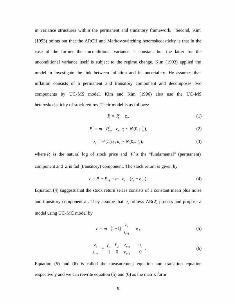
components by UC-MS model. Kim and Kim (1996) also use the UC-MS
heteroskedasticity of stock returns. Their model is as follows:
* ,t t tP P z= + (1)
* * 21 , ~ (0, ),t t t t etP P e e Nµ σ−= + + (2)
2( ) , ~ (0, ),t t t utz L u u N σ= Ψ (3)
where tP is the natural log of stock price and *tP is the “fundamental” (permanent)
component and tz is fad (transitory) component. The stock return is given by
1 1( ).t t t t t tr P P e z zµ− −= − = + + − (4)
Equation (4) suggests that the stock return series consists of a constant mean plus noise
and transitory component tz . They assume that tz follows AR(2) process and propose a
model using UC-MC model by
1
[1 1] ,tt t
t
zr e
zµ
−
= + − +
(5)
11 2
1 2
.1 0 0
t t t
t t
z z uz z
φ φ −
− −
= +
(6)
Equation (5) and (6) is called the measurement equation and transition equation
respectively and we can rewrite equation (5) and (6) as the matrix form

10
t t ty H eµ β= + + (7)
1t t tF vβ β −= + (8)
where Markov-switching variances are two shocks related to the permanent and
transitory components.
2 2 21 1 1(1 ) ,et t et t eS Sσ σ σ= − + (9)
2 2 22 0 21(1 ) ,ut t u utS Sσ σ σ= − + (10)
where the two independent unobserved state variables, 1tS and 2tS , evolve according to
first order, discrete, two-state Markov processes with following transition probabilities
which determine the regime.
[ ] [ ]1 1 1 00 1 1 1 11Pr 0 | , 0 ,P r 1 | , 1t t t tS S p S S p− −= = = = = =
2 2, 1 00 2 2, 1 11Pr 0 | 0 ,Pr 1 | 1t t t tS S q S S q− −= = = = = = (11)
We can estimate the parameters by Kalman filter and Kim (1993)’s mixed collapsing
method. For more detail estimation procedure, refer to Kim and Kim (1996), and Kim
and Nelson (1998).
To identify the permanent and transitory component and its relationship within
GCC countries, we set the model as follows:
t t tr cτ= + (12)
0 1 1( ) , (0,1),t t t tQ Q S Nτ µ ε ε= + + : (13)
0 1 2( ) ( ) , (0,1),t t t tL c h h S e e Nφ = + : (14)
where tτ is the permanent part of the return and tc is the transitory (or temporary) part of
the return and we assume that it follows AR(1) process. The parameter 1h and 1Q indicate
11
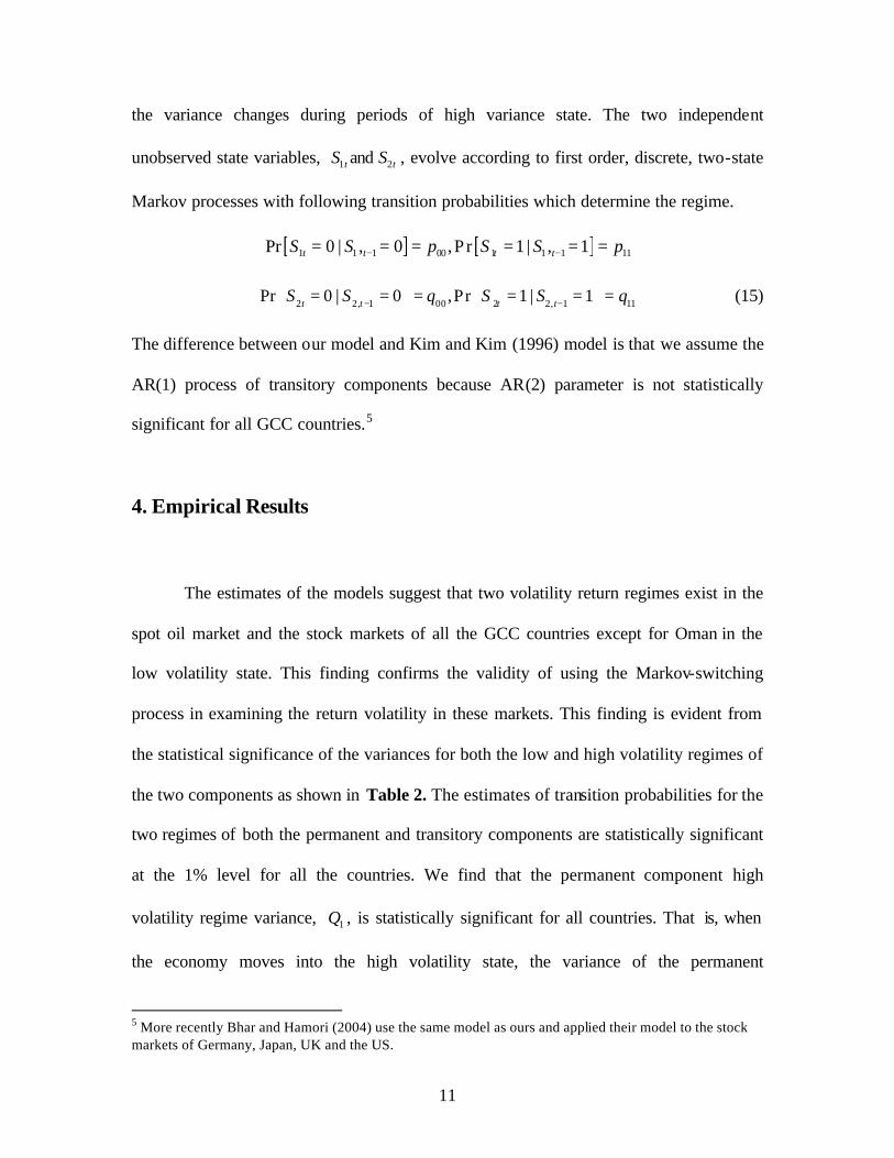
the variance changes during periods of high variance state. The two independent
unobserved state variables, 1tS and 2tS , evolve according to first order, discrete, two-state
Markov processes with following transition probabilities which determine the regime.
[ ] [ ]1 1 1 00 1 1 1 11Pr 0 | , 0 ,P r 1 | , 1t t t tS S p S S p− −= = = = = =
2 2, 1 00 2 2, 1 11Pr 0 | 0 ,Pr 1 | 1t t t tS S q S S q− −= = = = = = (15)
The difference between our model and Kim and Kim (1996) model is that we assume the
AR(1) process of transitory components because AR(2) parameter is not statistically
significant for all GCC countries.5
4. Empirical Results
The estimates of the models suggest that two volatility return regimes exist in the
spot oil market and the stock markets of all the GCC countries except for Oman in the
low volatility state. This finding confirms the validity of using the Markov-switching
process in examining the return volatility in these markets. This finding is evident from
the statistical significance of the variances for both the low and high volatility regimes of
the two components as shown in Table 2. The estimates of transition probabilities for the
two regimes of both the permanent and transitory components are statistically significant
at the 1% level for all the countries. We find that the permanent component high
volatility regime variance, 1Q , is statistically significant for all countries. That is, when
the economy moves into the high volatility state, the variance of the permanent
5 More recently Bhar and Hamori (2004) use the same model as ours and applied their model to the stock markets of Germany, Japan, UK and the US.

12
component of the return increases for those countries significantly. We can evaluate the
magnitude of the overall variance of the permanent component variances by the adding
the low and high state variances. The permanent component of oil price return shows the
highest variance.
The estimates of the parameters of the weekly transitory component suggest
several implications. First, the transitional probability for both high and low volatility
regimes are statistically significant for all countries and the oil price returns. Second, in
our sample, the transitory low variance state, 00q is higher than 11q which suggest that the
low volatility state dominates the high volatility state. In other words, the transitory shock
is short lived. The expected durations of the high volatility state (of transitory
component) for Bahrain, Kuwait, Oman, UAE, and Saudi are 22.2, 62.5, 7.0, 4.6 and 3.4
weeks, respectively as shown in Table 3, having an average of about 19.9. On the other
hand, the expected durations of the low volatility state (of transitory component) for
Bahrain, Kuwait, Oman, UAE, and Saudi are 66.7, 250.0, 15.2, 18.5 and 27.0 weeks,
respectively, having an average of about 75.4 weeks. The high volatility state variance is
higher than the low volatility state variance for all countries and it is clear that during the
high volatility state the uncertainty is much higher for those stock markets.
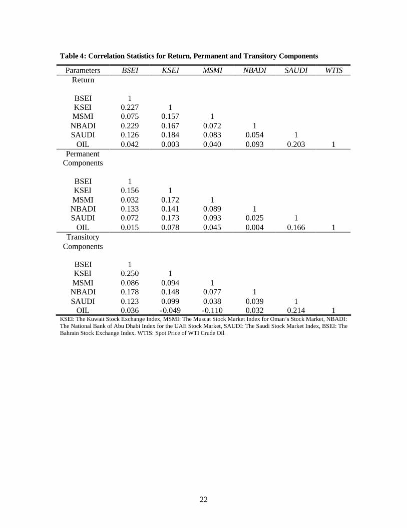
Table 4 shows the weekly correlation patterns for the return itself and its
permanent and transitory components between individual GCC countries. The correlation
patterns are positive for all the three returns measures, implying that these returns move
together in the short- and long-runs. This should not be surprising because these countries
are located in the same geographical region and share many common social and
economic characteristics including high dependence on the oil revenues. The highest

13
correlation in returns is between Bahrain and UAE (0.229), and between Bahrain and
Kuwait (0.227), implying that these two countries have the highest, same direction
movements in returns which makes these markets the least eligible candidates among the
GCC markets for portfolio diversification. Kuwaiti and UAE companies are listed on the
Bahrain stock Exchange. Still these return correlations are significantly low if compared
to those between Germany, Japan, UK and the US as reported in Bhar and Hamori
(2004), in the light of the GCC ‘s high dependence on oil. The lowest return correlation is
between Saudi and UAE (0.054), implying that these two countries are better candidate to
be combined in diversification-based portfolios when returns are in the high volatility
regime. However, the correlations for the permanent components provide different
results. The highest fundamental correlation is between Kuwait and Saudi Arabia (0.173).
This may be explained by the relatively high correlation between these countries’
fundamentals and that of the oil price. The lowest fundamental correlation is between
Saudi Arabia and UAE. In contrast to Saudi Arabia, the UAE fundamental has very low
correlation with the oil price returns. In terms of the transitory component, the highest
correlation is between Bahrain and Kuwait (0.250), and the lowest is between Oman and
Saudi Arabia (0.038).
As mentioned above, the GCC weekly return correlations with the oil spot price
return are surprisingly low for all GCC countries. This means that the oil price is only
one factor that moves the GCC stock markets on a weekly basis. The highest correlation
with the oil price return is for Saudi Arabia, which is the largest oil exporter in the world.
This correlation in terms of: the stock return itself is 0.203; the fundamental is 0.166; and
the transitory is 0.214. The lowest oil correlation for the fundamental is for UAE which is
14
also affected by regional tourism as well as by oil revenues. UAE has only one emirate
among its six united emirates that is a major oil exporter. It is surprising that Kuwait has
the lowest correlation for the return itself. However, it is possible that on weekly basis
and in a market that is highly sensitive to fads that the oil connection is weak.
5. Conclusions
Since the study clearly shows that there exist two volatility regimes in the two
components of all stock returns of the GCC countries, then risk-averse investors should
demand different compensations depending on the state of the economy and the shocks in
the components. Those GCC investors should ask for higher compensation in the high
volatility state regardless whether the shock hits the fundaments or the fads. Moreover,
sensitivity to return volatility during fad times is much higher than the volatility
sensitivity due to shocks in the fundamentals regardless of the return regime. It seems
that at times of increases in fads and speculative attacks noisy traders experience changes
in price misperceptions and that considerably increases the risk in all the GCC markets.
Thus those investors should ask for much higher premiums during fad times. .
Since sensitivity to return volatility varies across the GCC markets depending on
the state of the economy and the component of the return, the risk-averse investors in the
Oman market should particularly ask for the highest premium among the five GCC
markets during the high volatility state of the fad component, followed by investors in the
Saudi and the UAE markets. The Omani market should consider introducing financial
hedge instruments that can protect investors during fad times. The lowest fad premium

15
should go to investors in the Bahrain market which is more integrated with the world
stock market than the other GCC markets.
The spot oil market plays a very important factor in determining the returns of the
GCC stocks particularly during changes in the fundamentals and the fads. The additional
oil variance for both components is higher than that fo r most of the GCC markets. This
may explain why Bahrain, which is basically a non oil producing country, has the lowest
volatility sensitivity during fads.
The GCC markets also vary in the duration of volatility across regimes and for the
two components. Oman and Saudi Arabia have longer volatility durations as a result of
shocks in the fundaments such as the oil market than all those markets. In this case risk–
averse investors and traders in these two countries should opt for longer term investments
than in the other market to ride the volatility. Macroeconomic policy makers in these
countries should also be aware of the longer volatility and makes policies in times of fads
that stabilize the stock markets especially during speculative attacks in the oil market.
In terms of movements of the returns, all GCC returns move in the same direction
whether in terms of total return, fundamentals or fads under both volatility regimes,
suggesting that they are commoved by a common factor such as political stability,
liquidity and/or the oil price in the short and long-runs. The highest movements are
between Kuwait and Bahrain, and Bahrain and UAE which makes these markets the least
eligible candidates for portfolio diversification among the GCC markets. There are also
relatively high correlation between Kuwait and Saudi Arabia. Overall the correlations
among the GCC whether in terms of to the return itself, the fundamental and the fad are
low, suggesting that these countries are very different when it comes to return on

16
financial investment. Thus, investors should do their homework before investing in these
countries. Saudi Arabia has the highest correlation with the spot oil price but in general
the oil correlation weak, confirming the above point that there are country particularities
that influence the stock returns in addition to the oil price.
17
References:
Bhar, R. and Hamori, S. 2004. Empirical characteristics of the permanent and transitory components of stock returns: Analysis in a Markov-switching heteroscedasticity framework. Economic letters, forthcoming. Campbell, J. Y and Mankiew, N. G. 1987. Are output fluctuation transitory? Quarterly Journal of Economics 102, 857-880. Chu, C.-S., Santoni, G. J., and Liu, T. 1996. Stock market volatility and regime shifts in returns. Information Sciences 94, 179-190. Clark, P. K. 1987. The cyclical component of the US economic activity, Quarterly Journal of Economics 102, 797-814. De Lond, J. B., Shleifer, A., L. H., Summes, L. H. and Waldmann, R. J., 1990. Noise trader risk in financial markets. Journal of political economy, 98, 703-738. Fama, E. F. and French, K. R. 1988. Permanent and temporary components of stock prices. Journal of political economy, 96, 246-273. Glosten, L. K., Jagannathan, R. and Runkle, D. E. 1993. On the relation between the expected value and the volatility of the nominal excess return on stocks. Journal of Finance 48(5), 1779-1801. Hamilton, J. D. 1989. A new approach to the economic analysis of nopnstationary time series and the business cycle. Econometrica 57(2), 357-384. Hamilton J.D. and Susmel, R., 1994. Autoregressive conditional heteroscedasticity and changes in regime. Journal of Econometrics 64, 307–333. Hammoudeh, S. and Elesia, E. 2004. Dynamic relationships among GCC stock markets and NYMEX oil futures. Contemporary Economic Policy 22 (2), 250-269.
Hammoudeh, S. and Malik, F. 2004, Shock and volatility transmission in the NYMEX oil, US and Gulf equity markets. Paper presented at the Middle East Economic Association Meeting, San Diego, CA. Harvey, C. R. znd A. Siddique, 1999. Autoregressive conditional skewness. Journal of Financial Quantitative Analysis 43, 465 –487. Kim, C. J. 1993. Unobserved-component time series models with Markov-switching: Changes in regime and the link between inflation rates and inflation uncertainty. Journal of Business and Economic Statistics 11, 341-349.
18
Kim, C.J., and Kim, M. J. 1996. Transient fads and the crash of ’87. Journal of Applied Econometrics 11, 41-58. Kim, C. J., and Nelson, C. R. 1999. State Space Models with Regime Switching, Classical and Gibbs Sampling Approach with Application. The MIT Press, Cambridge, MA. Nelsson, C. R., and Plosser, C. I. 1982. Trends and Random walks in macroeconomic time series: Some evidence and implications. Journal of Monetary Economics 10, 139-162. McCarthy, J. and Najand, N.1995. State space modeling of linkages among international markets. Journal of Multinational Financial Management 5, 1-9. Porterba, J. M. and Summers, L. H. 1988. Mean reversion in stock prices: Evidence and implications. Journal of Financial Economics 22, 27-59. Schaller, H. and van Norden, S. 1997. Regime-switching in stock market returns. Applied Financial Economics 7, 177-191. Turner, R. F., Startz, R. and Nelson, C. F. 1989. A Markov model of heteroskedasticity, risk, and learning in the stock market, Journal of Financial Economics. 25, 3-22 . Watson, M. W. 1986.Univariate detrending methods with stochastic trends. Journal of Monetary Economics 18, 49-75.

19
Table 1: Descriptive Statistics of the GCC Stock Index and Spot Oil Price Returns
Notes: All variables are first differences of logs, and thus they represent rates of return. KSEI: The Kuwait Stock Exchange Index, MSMI: The Muscat Stock Market Index for Oman’s Stock Market, NBADI: The National Bank of Abu Dhabi Index for the UAE Stock Market, SAUDI: The Saudi Stock Market Index, BSEI: The Bahrain Stock Exchange Index. WTIS: Spot Price of WTI Crude Oil. a C.V. is called Coefficient of Variation, which is defined as the standard deviation divided by the mean.
Statistics BSEI KSEI MSMI NBADI SAUDI DOWI WTIS
Mean 0.983 1.612 1.927 1.329 1.002 1.972 21.121
Maximum 1.418 2.783 4.376 2.463 1.528 2.943 36.750
Minimum 0.679 0.393 1.000 0.878 0.675 0.921 10.860
Std. Dev. 0.192 0.482 0.767 0.338 0.223 0.664 5.460
C.Va 0.195 0.299 0.398 0.254 0.223 0.337 0.259
Skewness 0.149 0.610 1.387 0.979 0.596 -0.216 0.570
Kurtosis 1.885 2.655 4.319 3.601 2.123 1.572 2.702
Jarque-Bera 22.802 27.550 161.648 71.874 37.503 38.119 23.800
Probability 0.000 0.000 0.000 0.000 0.000 0.000 0.000

20
Table 2: Estimation of Permanent and Transitory Components of GCC Stock Return
Parameters BSEI KSEI MSMI NBADI SAUDI WTIS 0µ̂ -0.042
(0.049) 0.057
(0.090) 0.130
(0.093) 0.038
(0.065) 0.127
(0.089) 0.156 (0.207)
φ 0.320a (0.090)
0.323b (0.136)
0.343a (0.084)
0.747a (0.066)
0.211 (0.208)
-0.219b (0.109)
0Q 0.001 (0.001)
0.469 (0.335)
0.711a (0.083)
0.175a (0.038)
0.899c (0.528)
1.362 (1.177)
1Q 1.754a (0.226)
1.088a (0.241)
0.770a (0.083)
0.747a (0.137)
0.885a (0.289)
2.303b (0.913)
0h 0.602a (0.045)
0.802a (0.231)
0.001 (0.001)
0.199a (0.026)
0.900c (0.528)
1.674c (0.919)
1h 1.247a (0.258)
1.140a (0.372)
3.829a (0.361)
2.292a (0.372)
2.713a (0.703)
3.638a (0.849)
11p̂ 0.789a (0.126)
0.959a (0.029)
0.997a (0.004)
0.944a (0.033)
0.989a (0.010)
0.996a (0.005)
00p̂ 0.904a (0.038)
0.951a (0.031)
0.986a (0.011)
0.949a (0.028)
0.995a (0.005)
0.973a (0.020)
11q̂ 0.955a (0.042)
0.984a (0.016)
0.857a (0.070)
0.782a (0.101)
0.706a (0.119)
0.973a (0.018)
00q̂ 0.985a (0.016)
0.996a (0.005)
0.934a (0.028)
0.946a (0.022)
0.963a (0.022)
0.975a (0.015)
Log Likelihood 651.39 766.77 854.21 508.02 817.83 1229.58 Note that a, b and c denotes rejection of the hypothesis at the 1%, 5% and 10% levels respectively. Standard errors are given in parentheses below the parameter estimates. BSEI: The Bahrain Stock Exchange Index, KSEI: The Kuwait Stock Exchange Index, MSMI: The Muscat Stock Market Index for Oman’s Stock Market, NBADI: The National Bank of Abu Dhabi Index for the UAE Stock Market, SAUDI: The Saudi Stock Market Index, WTIS: Spot Price of WTI Crude Oil.

21
Table 3: Volatility Duration for Permanent and Transitory Components
Duration BSEI KSEI MSMI NBADI SAUDI WTIS Permanent Components
Low volatility 10.42 20.41 71.43 19.61 16.67 37.04 High volatility 4.74 24.5 333.33 17.86 90.91 250.00
Transitory Components
Low volatility 66.67 250.00 15.15 18.52 27.03 40.00 High volatility 22.22 62.50 6.99 4.59 3.40 37.03
Notes: Duration is measured in weeks as 1/(1- probability). BSEI: The Bahrain Stock Exchange Index., KSEI: The Kuwait Stock Exchange Index, MSMI: The Muscat Stock Market Index for Oman’s Stock Market, NBADI: The National Bank of Abu Dhabi Index for the UAE Stock Market, SAUDI: The Saudi Stock Market Index, WTIS: Spot Price of WTI Crude Oil.
22
Table 4: Correlation Statistics for Return, Permanent and Transitory Components
Parameters BSEI KSEI MSMI NBADI SAUDI WTIS Return
BSEI 1 KSEI 0.227 1 MSMI 0.075 0.157 1 NBADI 0.229 0.167 0.072 1 SAUDI 0.126 0.184 0.083 0.054 1
OIL 0.042 0.003 0.040 0.093 0.203 1 Permanent
Components
BSEI 1 KSEI 0.156 1 MSMI 0.032 0.172 1 NBADI 0.133 0.141 0.089 1 SAUDI 0.072 0.173 0.093 0.025 1
OIL 0.015 0.078 0.045 0.004 0.166 1 Transitory
Components
BSEI 1 KSEI 0.250 1 MSMI 0.086 0.094 1 NBADI 0.178 0.148 0.077 1 SAUDI 0.123 0.099 0.038 0.039 1
OIL 0.036 -0.049 -0.110 0.032 0.214 1 KSEI: The Kuwait Stock Exchange Index, MSMI: The Muscat Stock Market Index for Oman’s Stock Market, NBADI: The National Bank of Abu Dhabi Index for the UAE Stock Market, SAUDI: The Saudi Stock Market Index, BSEI: The Bahrain Stock Exchange Index. WTIS: Spot Price of WTI Crude Oil.