Volatility in the Indian Financial Market Before, During ... · Volatility in the Indian Financial...

Volatility in the Indian Financial Market Before, During and After the Global Financial Crisis

Praveen Kulshreshtha

Indian Institute of Technology Kanpur, India

Aakriti Mittal Indian Institute of Technology Kanpur, India

The ARCH/GARCH time series models are employed to examine the volatility in the Indian financial market during 2000-14, by using all eight Indian stock indices, i.e. BSE SENSEX, BSE 100, BSE 200, BSE 500, CNX NIFTY, CNX 100, CNX 200 and CNX 500. The impact of the global financial crisis on the volatility of returns is analyzed by splitting the time series into three phases: the pre-crisis period (2000-06), the crisis period (2007-10) and the post-crisis period (2011-14). The best fitted model is used to predict the conditional variance of the differenced series of returns, which is found to be stationary. INTRODUCTION

The US housing bubble burst of 2008 had serious economic consequences not only in the USA, but also in many developing and emerging economies such as India. The crisis also affected financial markets globally. From 2004 to 2007, the volatility in the US financial market, as measured by S&P 500 volatility and the Chicago Board Options Exchange Market Volatility Index (VIX), was below the long-term average (Manda, 2010). However, the global financial crisis of 2008 led to a sharp decline in asset prices, the correlation between asset prices increased significantly and global financial markets (for instance, the Indian stock market) became extremely volatile, as highlighted by the following facts (Manda, 2010; Thomas, 2009):

(a) 2008 owners of stocks in the USA suffered losses of about $8 trillion, as the value of stocks declined from $20 trillion to $12 trillion.

(b) S&P 500 lost about 56% of its value, from its peak of October, 2007 to the trough of March, 2009.

(c) During the crisis, VIX volatility index more than tripled. (d) There was a huge withdrawal from the Indian stock market, mainly by the Foreign Institutional

Investors (FIIs). This led to a net outflow of portfolio investments in the Indian stock market, to the tune of $16 billion, between February, 2008 and September, 2008.

High volatility in a financial market creates a great degree of uncertainty regarding returns from

financial investment, and hence, leads to a large degree of risk associated with investment in the market. Investors are hesitant to make heavy investments in stocks and their savings can be adversely affected. Low investment in stocks results in lack of availability of funds for businesses, which are thus unable to

Journal of Accounting and Finance Vol. 15(3) 2015 141

procure productive capital easily. Hence, high volatility in a financial market lowers productive investment in an economy and the growth of the economy is adversely affected. Therefore, it is important to study the volatility in a financial market, both in the short-run and long-run. Also, a study of volatility is very important for proper formulation of economic policies related to financial markets.

Volatility in the financial markets has been analyzed extensively for developed countries as well as for developing economies such as India. However, in studies pertaining to the volatility in the Indian financial market, little emphasis has been laid on studying and comparing the volatility in all the stock price indices of the country’s two stock exchanges, namely, Bombay Stock Exchange (BSE) and National Stock Exchange (NSE).

In this study, we focus on analyzing and comparing the volatility of returns in each of the eight Indian stock price indices, namely, BSE SENSEX, BSE 100, BSE 200, BSE 500, CNX NIFTY, CNX 100, CNX 200 and CNX 500, during 2000-14. We also analyze the impact of the global financial crisis on the volatility of returns in India’s two premier stock indices, namely, BSE SENSEX and CNX NIFTY. To accomplish this, we split the BSE SENSEX and CNX NIFTY time series into three phases: the pre-crisis period (2000-06), the crisis period (2007-10) and the post-crisis period (2011-14).

A sound empirical analysis of market volatility requires an appropriate econometric model that helps explain the changes in asset prices over time. The Autoregressive Conditional Heteroskedasticity (ARCH) and Generalized Autoregressive Conditional Heteroskedasticity (GARCH) time series models can elucidate the volatility in a financial time series and its characteristics such as volatility clustering (Zivot and Wang, 2006). Therefore, we use the ARCH and GARCH models to analyze the volatility in the Indian financial market.

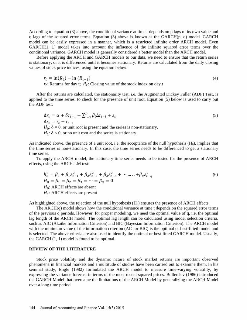
Volatility clustering refers to the tendency of asset prices to fluctuate in manner such that large changes (of either sign) in asset prices follow large changes, while small changes (of either sign) in asset prices follow small changes. This feature is clearly exhibited in the Indian financial market, as illustrated by Table 1, Figure 1 and Figure 2 below, which plot the daily returns of BSE SENSEX and CNX NIFTY stock indices during 2000-14:

TABLE 1 TALLY OF DAY-WISE REPRESENTATION WITH CORRESPONDING YEARS

Representation Years

0-1000 2000-04 1000-2000 2004-08 2000-3000 2008-12 3000-4000 2012-14

FIGURE 1

PLOT OF DAILY RETURNS OF BSE SENSEX

142 Journal of Accounting and Finance Vol. 15(3) 2015

FIGURE 2 PLOT OF DAILY RETURNS OF CNX NIFTY

The rest of the paper is organized as follows: The next section describes the methodology of time series modeling and analysis that is used in the study. The relevant literature is reviewed in Section 3. The results of our empirical analysis are presented and discussed in Section 4. Lastly, Section 5 concludes the paper. METHODOLOGY OF TIME SERIES MODELING AND ANALYSIS

To model financial time series and stylized facts such as volatility clustering, the ARCH model is found to be suitable. It can be easily observed from Figures 1 and 2 above that the current and previous levels of volatility are positively correlated. The correlation, or rather, autocorrelation (as the values of same variable at different points of time are correlated) can be parameterized using the ARCH model, which expresses the conditional variance of the error term as a function of the previous values of the squared error term.

𝑦𝑡 = 𝛼1 + 𝑢𝑡 𝑢𝑡~𝑁(0,ℎ𝑡2) (1) ℎ𝑡2 = 𝛽0 + 𝛽1𝜀𝑡−12 + 𝛽2𝜀𝑡−22 + 𝛽3𝜀𝑡−32 + ⋯… . . +𝛽𝑞𝜀𝑡−𝑞2 (2)

Equation (1) above depicts the basic regression equation, in which yt is the dependent variable, which represents the daily returns in terms of a given stock index, and ut depicts the random error term. Also, conditional on the information available at time (t-1), the random error term ut is normally distributed, with zero mean and variance ht

2 (which is referred to as the conditional variance of ut). Equation (2) above postulates that the conditional variance of the random error term ut (ht

2) depends on q lags of the squared error terms (εt-q

2). The above model is referred to as the ARCH(q) model. As the conditional variance (ht

2) and the squared error terms (εt-q2) are always non-negative, it is required that all the

coefficients of the squared error terms in equation (2) above (i.e. β1, β2,…, βq) are non-negative, so that the conditional variance is always non-negative.

The GARCH model expresses the conditional variance of the random error term (ht2) as a function of

its own past values and the squared error terms of previous periods, as illustrated by the equation below:

ℎ𝑡2 = 𝛽0 + 𝛽1𝜀𝑡−12 + 𝛽2𝜀𝑡−22 + 𝛽3𝜀𝑡−32 + ⋯+ 𝛽𝑞𝜀𝑡−𝑞2 + 𝛾1ℎ𝑡−12 + 𝛾2ℎ𝑡−22 + ⋯+ 𝛾𝑝ℎ𝑡−𝑝2 (3)


According to equation (3) above, the conditional variance at time t depends on p lags of its own value and q lags of the squared error terms. Equation (3) above is known as the GARCH(p, q) model. GARCH model can be easily expressed in a manner, which is a restricted infinite order ARCH model. Even GARCH(1, 1) model takes into account the influence of the infinite squared error terms over the conditional variance. GARCH model is generally considered a better model than the ARCH model.

Before applying the ARCH and GARCH models to our data, we need to ensure that the return series is stationary, or it is differenced until it becomes stationary. Returns are calculated from the daily closing values of stock price indices, using the equation below:

𝑟𝑡 = ln(𝑅𝑡) − ln (𝑅𝑡−1) (4) 𝑟𝑡: Returns for day t; 𝑅𝑡: Closing value of the stock index on day t

After the returns are calculated, the stationarity test, i.e. the Augmented Dickey Fuller (ADF) Test, is

applied to the time series, to check for the presence of unit root. Equation (5) below is used to carry out the ADF test:

∆𝑟𝑡 = 𝛼 + 𝛿𝑟𝑡−1 + ∑ 𝛽𝑖∆𝑟𝑡−𝑖𝑝𝑖=1 + 𝜀𝑡 (5)

∆𝑟𝑡 = 𝑟𝑡 − 𝑟𝑡−1 𝐻0: δ = 0, or unit root is present and the series is non-stationary. 𝐻1: δ < 0, or no unit root and the series is stationary.

As indicated above, the presence of a unit root, i.e. the acceptance of the null hypothesis (H0), implies that the time series is non-stationary. In this case, the time series needs to be differenced to get a stationary time series.

To apply the ARCH model, the stationary time series needs to be tested for the presence of ARCH effects, using the ARCH-LM test:

ℎ𝑡2 = 𝛽0 + 𝛽1𝜀𝑡−12 + 𝛽2𝜀𝑡−22 + 𝛽3𝜀𝑡−32 + ⋯… . . +𝛽𝑞𝜀𝑡−𝑞2 (6) 𝐻0 = 𝛽1 = 𝛽2 = 𝛽3 = ⋯ = 𝛽𝑞 = 0 𝐻0: ARCH effects are absent 𝐻1: ARCH effects are present

As highlighted above, the rejection of the null hypothesis (H0) ensures the presence of ARCH effects.

The ARCH(q) model shows how the conditional variance at time t depends on the squared error terms of the previous q periods. However, for proper modeling, we need the optimal value of q, i.e. the optimal lag length of the ARCH model. The optimal lag length can be calculated using model selection criteria, such as AIC (Akaike Information Criterion) and BIC (Bayesian Information Criterion). The ARCH model with the minimum value of the information criterion (AIC or BIC) is the optimal or best-fitted model and is selected. The above criteria are also used to identify the optimal or best-fitted GARCH model. Usually, the GARCH (1, 1) model is found to be optimal. REVIEW OF THE LITERATURE

Stock price volatility and the dynamic nature of stock market returns are important observed phenomena in financial markets and a multitude of studies have been carried out to examine them. In his seminal study, Engle (1982) formulated the ARCH model to measure time-varying volatility, by expressing the variance forecast in terms of the most recent squared prices. Bollerslev (1986) introduced the GARCH Model that overcame the limitations of the ARCH Model by generalizing the ARCH Model over a long time period.


Several researchers have studied the volatility in the financial markets before, during or after the recent global financial crisis. Manda (2010) analyzed the impact of the global financial crisis on the stock market volatility in the USA. She found that the stock market in USA was relatively calm during 2004 to 2007, i.e. before the global financial crisis, since the market volatility, as captured by the volatility in the S&P 500 and VIX indices, remained below the long-term average during the above period. However, she found that the market volatility in USA increased significantly during the global financial crisis.

Similarly, many researchers have analyzed the volatility in the Indian financial market, before, during or after the global financial crisis. Pandey (2003) compared the performances of conditional and unconditional volatility estimators by analysing high frequency data pertaining to the CNX NIFTY stock index, collected over a period of 3 years (1999-2001). The results showed that although the conditional estimators were less biased, the unconditional extreme-value estimators were more efficient and their forecasts were better than the forecasts based on the conditional estimators.

Karmakar (2005) forecasted the volatility in the Indian financial market using the GARCH (1, 1) model, which was found to be the best fitting model for data pertaining to BSE SENSEX and CNX NIFTY stock indices. He also evaluated the model individually for all the 50 companies included in the CNX NIFTY stock index and observed that the model captured the stylized facts concerning the volatility in the Indian stock market, such as leverage effect and volatility clustering, quite accurately.

Kumar (2006) analyzed the Indian stock and forex markets with the help of 10 volatility forecasting models, and compared their performance on the basis of symmetric and asymmetric errors. His results showed that GARCH (4, 1) and GARCH (5, 1) models performed well for the Indian stock market and forex market respectively. Goudarzi and Ramanarayanan (2010) used the BSE 500 stock index, sampled over a period of 10 years, to study the volatility in the Indian stock market. They incorporated various features of the Indian stock market volatility, such as fat tails and volatility clustering, through the GARCH (1, 1) model.

Mishra (2010) studied the stock return volatility in the Indian capital market during 1991-2009 by using GARCH models. He observed that sudden changes in market volatility pose greater danger to the economic and financial stability of India than sustained changes in the Indian capital market. He found the Threshold GARCH (TGARCH) model to be the most suitable for predicting the volatility in the Indian capital market.

Chakrabarti and Nathan (2013) worked with autoregressive neural networks and forecasted the daily volatility in the Indian capital market with higher accuracy as compared to the GARCH(1, 1) model. They also observed that only 5-6 lag periods were sufficient to predict the market volatility efficiently. On the other hand, Vijayalaxmi and Gaur (2013) examined the BSE and NSE stock price indices, and attempted to capture the asymmetry and volatility of the financial market through the best fitting model. They found that the Threshold ARCH model (TARCH) and the Power ARCH model (PARCH) were the best fitting models. DATA, RESULTS AND INTERPRETATION

Daily closing values of all the eight Indian stock price indices, i.e. BSE SENSEX, BSE 100, BSE 200, BSE 500, CNX NIFTY, CNX 100, CNX 200 and CNX 500, were collected for the period 2000-14, using the NSE database (http://www.nseindia.com/), the BSE database (http://www.bseindia.com/) and Yahoo Finance (https://in.finance.yahoo.com/). More specifically, over 3500 daily observations of each stock index, spanning the period January, 2000 to May, 2014, were used for the analysis. Returns were calculated using equation (4) above. The STATA statistical package was used to conduct the time series data analysis.

The time series for all eight stock indices were tested for stationarity using the ADF test and were found to be non-stationary. Therefore, each stock index time series was differenced to obtain a stationary time series. The ARCH LM test was carried out for all differenced time series, which showed that ARCH effects are present in all the eight stock index time series. Different lag lengths for the ARCH model were tried for each differenced time series. AIC and BIC were used to pick the optimal or best-fitted ARCH


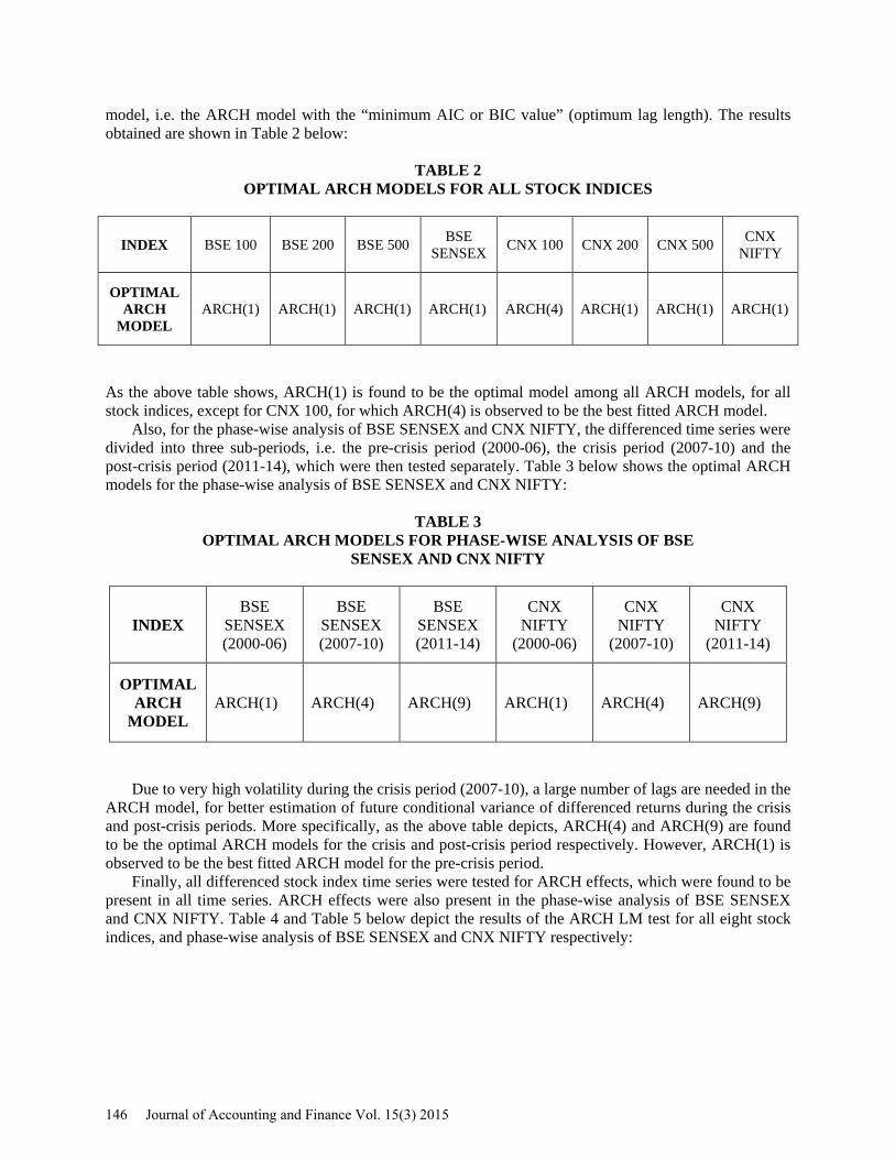
model, i.e. the ARCH model with the “minimum AIC or BIC value” (optimum lag length). The results obtained are shown in Table 2 below:

TABLE 2

OPTIMAL ARCH MODELS FOR ALL STOCK INDICES

INDEX BSE 100 BSE 200 BSE 500 BSE SENSEX CNX 100 CNX 200 CNX 500 CNX

NIFTY

OPTIMAL ARCH

MODEL ARCH(1) ARCH(1) ARCH(1) ARCH(1) ARCH(4) ARCH(1) ARCH(1) ARCH(1)

As the above table shows, ARCH(1) is found to be the optimal model among all ARCH models, for all stock indices, except for CNX 100, for which ARCH(4) is observed to be the best fitted ARCH model.

Also, for the phase-wise analysis of BSE SENSEX and CNX NIFTY, the differenced time series were divided into three sub-periods, i.e. the pre-crisis period (2000-06), the crisis period (2007-10) and the post-crisis period (2011-14), which were then tested separately. Table 3 below shows the optimal ARCH models for the phase-wise analysis of BSE SENSEX and CNX NIFTY:

TABLE 3

OPTIMAL ARCH MODELS FOR PHASE-WISE ANALYSIS OF BSE SENSEX AND CNX NIFTY

INDEX BSE

SENSEX (2000-06)

BSE SENSEX (2007-10)


CNX NIFTY

(2000-06)

CNX NIFTY

(2007-10)

CNX NIFTY

(2011-14)

OPTIMAL ARCH

MODEL ARCH(1) ARCH(4) ARCH(9) ARCH(1) ARCH(4) ARCH(9)

Due to very high volatility during the crisis period (2007-10), a large number of lags are needed in the ARCH model, for better estimation of future conditional variance of differenced returns during the crisis and post-crisis periods. More specifically, as the above table depicts, ARCH(4) and ARCH(9) are found to be the optimal ARCH models for the crisis and post-crisis period respectively. However, ARCH(1) is observed to be the best fitted ARCH model for the pre-crisis period.

Finally, all differenced stock index time series were tested for ARCH effects, which were found to be present in all time series. ARCH effects were also present in the phase-wise analysis of BSE SENSEX and CNX NIFTY. Table 4 and Table 5 below depict the results of the ARCH LM test for all eight stock indices, and phase-wise analysis of BSE SENSEX and CNX NIFTY respectively:


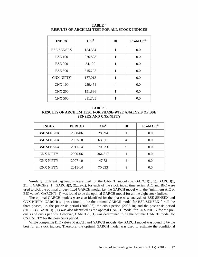
TABLE 4 RESULTS OF ARCH LM TEST FOR ALL STOCK INDICES

INDEX Chi2 Df Prob>Chi2

BSE SENSEX 154.334 1 0.0

BSE 100 226.828 1 0.0

BSE 200 34.129 1 0.0

BSE 500 315.205 1 0.0

CNX NIFTY 177.013 1 0.0

CNX 100 259.454 4 0.0

CNX 200 191.896 1 0.0

CNX 500 311.705 1 0.0

TABLE 5 RESULTS OF ARCH LM TEST FOR PHASE-WISE ANALYSIS OF BSE

SENSEX AND CNX NIFTY

INDEX PERIOD Chi2 Df Prob>Chi2

BSE SENSEX 2000-06 285.94 1 0.0

BSE SENSEX 2007-10 63.611 4 0.0

BSE SENSEX 2011-14 70.633 9 0.0

CNX NIFTY 2000-06 364.517 1 0.0

CNX NIFTY 2007-10 47.78 4 0.0

CNX NIFTY 2011-14 70.633 9 0.0

Similarly, different lag lengths were tried for the GARCH model (i.e. GARCH(1, 1), GARCH(1, 2),…, GARCH(2, 1), GARCH(2, 2),...etc.), for each of the stock index time series. AIC and BIC were used to pick the optimal or best-fitted GARCH model, i.e. the GARCH model with the “minimum AIC or BIC value”. GARCH(1, 1) was found to be the optimal GARCH model for all the eight stock indices.

The optimal GARCH models were also identified for the phase-wise analysis of BSE SENSEX and CNX NIFTY. GARCH(1, 1) was found to be the optimal GARCH model for BSE SENSEX for all the three phases, i.e. the pre-crisis period (2000-06), the crisis period (2007-10) and the post-crisis period (2011-14). GARCH(1, 1) was also identified as the optimal GARCH model for CNX NIFTY for the pre-crisis and crisis periods. However, GARCH(3, 1) was determined to be the optimal GARCH model for CNX NIFTY for the post-crisis period.

While comparing BIC values of ARCH and GARCH models, the GARCH model was found to be the best for all stock indices. Therefore, the optimal GARCH model was used to estimate the conditional


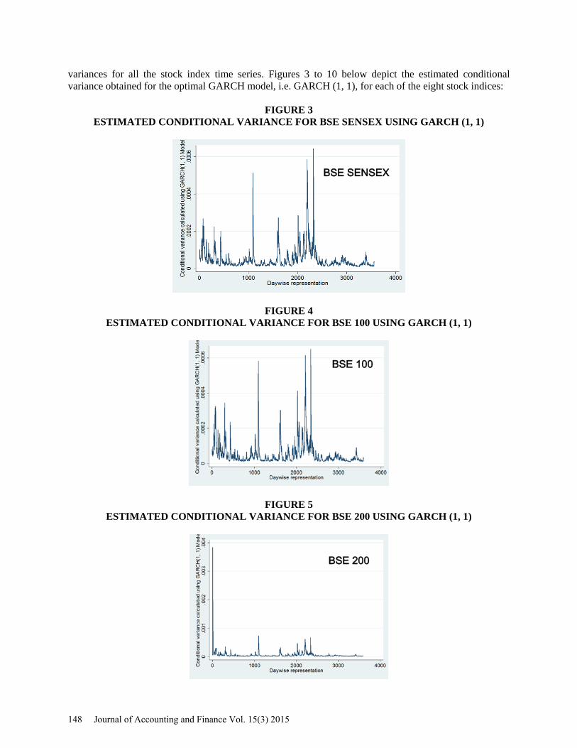
variances for all the stock index time series. Figures 3 to 10 below depict the estimated conditional variance obtained for the optimal GARCH model, i.e. GARCH (1, 1), for each of the eight stock indices:

FIGURE 3

ESTIMATED CONDITIONAL VARIANCE FOR BSE SENSEX USING GARCH (1, 1)

FIGURE 4 ESTIMATED CONDITIONAL VARIANCE FOR BSE 100 USING GARCH (1, 1)


BSE SENSEX

BSE 100

BSE 200



FIGURE 7 ESTIMATED CONDITIONAL VARIANCE FOR CNX NIFTY USING GARCH (1, 1)

FIGURE 8 ESTIMATED CONDITIONAL VARIANCE FOR CNX 100 USING GARCH (1, 1)

BSE 500

CNX NIFTY

CNX 100




Similarly, the optimal GARCH models were used to estimate the conditional variances for the BSE SENSEX and CNX NIFTY stock indices for the phase-wise analysis, during each of the three phases. The results are illustrated in Figures 11 to 16 below:

FIGURE 11

ESTIMATED CONDITIONAL VARIANCE FOR BSE SENSEX (2000-06) USING GARCH (1, 1)

CNX 500

CNX 200



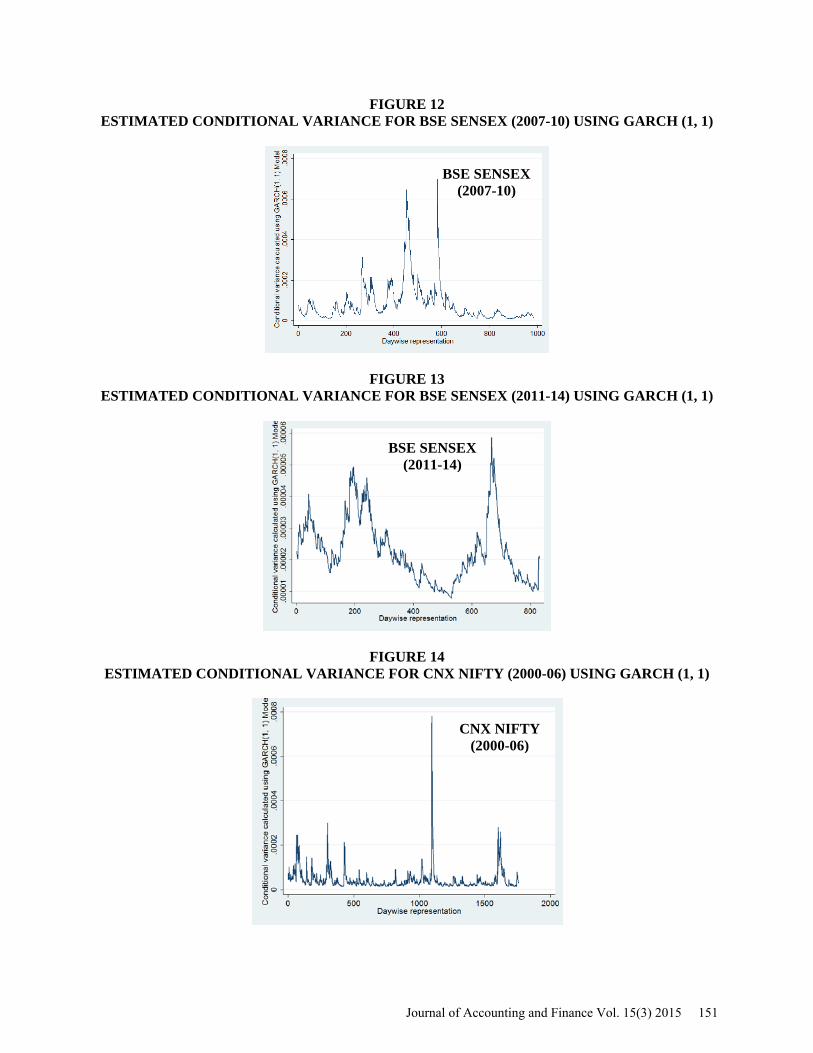
FIGURE 12 ESTIMATED CONDITIONAL VARIANCE FOR BSE SENSEX (2007-10) USING GARCH (1, 1)

FIGURE 13 ESTIMATED CONDITIONAL VARIANCE FOR BSE SENSEX (2011-14) USING GARCH (1, 1)

FIGURE 14 ESTIMATED CONDITIONAL VARIANCE FOR CNX NIFTY (2000-06) USING GARCH (1, 1)


CNX NIFTY (2000-06)





CONCLUSION

The study shows that ARCH effects are present in all differenced time series (which are stationary) for all the eight Indian stock indices, and hence, ARCH and GARCH modeling can be applied to study volatility in the Indian financial market, using the eight stock prices indices as the proxy for the Indian financial market. ARCH(1) is found to be the optimal model among all ARCH models, for all stock indices, except for CNX 100, for which ARCH(4) is observed to be the best fitted ARCH model. The study indicates that GARCH(1, 1) is the optimal GARCH model for all the eight Indian stock indices.

In the phase-wise analysis of BSE SENSEX and CNX NIFTY stock indices, GARCH(1, 1) is the optimal model for both stock indices in the three phases, except for the CNX NIFTY stock index in the post-crisis period (2011-14), for which GARCH (3, 1) is found to be the best fitted model. Due to very high volatility during the crisis period (2007-10), a large number of lags are needed in the ARCH model, for better estimation of future conditional variance during the crisis and post-crisis periods. More specifically, ARCH(4) and ARCH(9) are found to be the optimal ARCH models for the crisis and post-

CNX NIFTY (2007-10)

CNX NIFTY (2011-14)


crisis period respectively. However, ARCH(1) is observed to be the best fitted ARCH model for the pre-crisis period.

Thus, we can conclude that extreme volatility during the crisis period has affected the volatility in the Indian financial market for a long duration. The study focused on ARCH and GARCH models, but they cannot account for leverage effects, i.e. the tendency for volatility to increase more following a large price fall than following a price rise of the same magnitude, although they can account for volatility clustering in the stock index time series. Asymmetric GARCH modeling can be used to analyze the above effects. REFERENCES Bollerslev, T. (1986). Generalized autoregressive conditional heteroskedasticity. Journal of

Econometrics, 31, (3), 307-327. Chakrabarti, B. B. & Nathan, O. B. (2013). Estimating stock index volatility in India (IIM Calcutta

Working Paper 725). Kolkata, India: Indian Institute of Management, Calcutta. Retrieved from http://financelab.iimcal.ac.in/resdoc/WPS%20725.pdf

Engle, R. F. (1982). Autoregressive conditional heteroskedasticity with estimates of the variance of United Kingdom inflation. Econometrica, 50, (4), 987-1007.

Goudarzi, H. & Ramanarayanan, C. S. (2010). Modelling and estimation of volatility in the Indian stock market. International Journal of Business and Management, 5, (2), 85-98.

Karmakar, M. (2005). Modeling conditional volatility of the Indian stock markets. Vikalpa, 30, (3), 21-37.

Kumar, S. S. S. (2006). Forecasting volatility: Evidence from Indian stock and forex markets (IIM Kozhikode Working Paper 08/FIN/2006/06). Kozhikode, India: Indian Institute of Management, Kozhikode. Retrieved from https://www.iimk.ac.in/websiteadmin/FacultyPublications/ WorkingPapers/ForecastingVolatility.pdf

Manda, K. (2010). Stock market volatility during the 2008 financial crisis (Master’s thesis, New York University). Retrieved from https://www.stern.nyu.edu/sites/default/files/assets/documents /uat_024308.pdf

Mishra, P. K. (2010). A GARCH model approach to capital market volatility: The case of India. Indian Journal of Economics and Business, 9, (3), 631-641.

Pandey, A. (2003). Modeling and forecasting volatility in Indian capital markets (IIM Ahmedabad Working Paper 2003-08-03). Ahmedabad, India: Indian Institute of Management, Ahmedabad. Retrieved from http://www.iimahd.ernet.in/assets/snippets/workingpaperpdf/2003-08-03ajaypandey.pdf

Thomas, J. J. (2009). India and the global financial crisis: Some lessons and the way forward. Paper presented at Annual Money and Finance Conference, held at Indira Gandhi Institute of Development Research, Mumbai, India. Retrieved from http://www.igidr. ac.in/conf/money/mfc-11/Thomas_Jayan.pdf

Vijayalakshmi, S. & Gaur, S. (2013). Modeling volatility: Indian stock and foreign exchange markets. Journal of Emerging Issues in Economics, Finance and Banking, 2, (1), 583-598.

Zivot, E. & Wang, J. (2006). Modeling financial time series with s-plus (2nd ed.). New York, NY: Springer.


Volatility in the Indian Financial Market Before, During ... · Volatility in the Indian Financial...

Documents

Transcript of Volatility in the Indian Financial Market Before, During ... · Volatility in the Indian Financial...