Volatility. Downloads Today’s work is in: matlab_lec04.m Functions we need today: simsec.m,...
26
Volatility
-
Upload
ian-bainum -
Category
Documents
-
view
217 -
download
0
Transcript of Volatility. Downloads Today’s work is in: matlab_lec04.m Functions we need today: simsec.m,...

Volatility

Downloads
Today’s work is in: matlab_lec04.m
Functions we need today: simsec.m, simsecJ.m, simsecSV.m
Datasets we need today: data_msft.m

Homework 1
function r=simsec(mu,sigma,T);x=randn(T,1); for t=1:T; r(t,1)=exp(mu+sigma*x(t))-1;end;

Simulate Simple Process
>>data_msft;>>subplot(2,1,1); hist(msft(:,4),[-.2:.01:.2]);>>sigma=std(msft(:,4)); >>mu=mean(msft(:,4))-.5*sigma^2;
T=length(msft); >>r=simsec(mu,sigma,T);>>disp([mean(msft(:,4)) mean(r)]);>>disp([std(msft(:,4)) std(r)]);>>disp([skewness(msft(:,4)) skewness(r)]);>>disp([kurtosis(msft(:,4)) kurtosis(r)]);>>subplot(2,1,2); hist(r,[-.2:.01:.2]);


Compare simulated to actual
Mean, standard deviation, skewness match well
Kurtosis (extreme events) does not match well
Actual has much more mass in the tails (fat tails)
This is extremely important for option pricing!
CLT fails when tails are “too” fat

ModellingVolatility
How to make tales fatter? Add jumps to log normal distribution to
make tails fatter Jumps also help with modeling default Make volatility predictable: Stochastic volatility, governed by state
variable ARCH process (2003 Nobel prize, Rob
Engle)

Jumps
R(t)=exp(µ+σ*X(t)+J(t)) J(t)=J1 with p1, J2 with p2, 0 with 1-p1-p2
>>nlow=sum(msft(:,4)<-.1);>>nhigh=sum(msft(:,4)>.1);>>[T a]=size(msft);>>p1=nlow/T; p2=nhigh/T; >>J1=-.15; J2=.15;
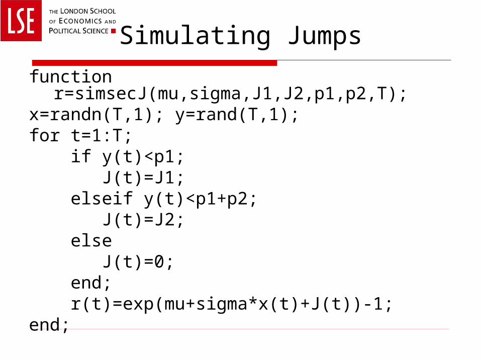
Simulating Jumps
function r=simsecJ(mu,sigma,J1,J2,p1,p2,T);x=randn(T,1); y=rand(T,1);for t=1:T; if y(t)<p1; J(t)=J1; elseif y(t)<p1+p2; J(t)=J2; else J(t)=0; end; r(t)=exp(mu+sigma*x(t)+J(t))-1;end;

Simulating Jumps
>>r=simsecJ(mu,sigma,J1,J2,p1,p2,T);>>disp([mean(msft(:,4)) mean(r)]);>>disp([std(msft(:,4)) std(r)]);>>disp([skewness(msft(:,4)) skewness(r)]);>>disp([kurtosis(msft(:,4)) kurtosis(r)]);>>subplot(2,1,2); hist(r,[-.2:.01:.2]); %Note that kurtosis of simulated now
matches actual


Stochastic Volatility
Suppose volatility was not constant, but changed through time and was predictable
This is very realistic, volatility tends to be much higher during recessions than expansions; high volatility tends to predict high volatility
That is sigma is replaced by sigma(t)=f(Z(t)) where Z(t) is a random variable

Moving Average
When we have a long time series of data we can calculate the local average a few points around each point in time, this is called a moving average
We will write code to calculate a moving average and use it to analyze stochastic volatility (to be used later as well)

Moving Average
>>T1=floor(T/7); ma=zeros(T1,2);>>for i=1:T1; in=(i-1)*7+1:(i-1)*7+7; ma(i,1)=std(msft(in,4)); ma(i,2)=mean(msft(in,4).^2); for j=1:7; t=(i-1)*7+j; ma(i,2)=ma(i,2)+(msft(t,4)^2)/7; end; end;>>disp(corrcoef(ma(:,1),ma(:,2)));

>>subplot(3,1,1); plot(ma(:,1));>>subplot(3,1,2); plot(ma(:,2));>>WN=exp(randn(T1,1)); subplot(3,1,3); plot(WN);

regress()
regcoef=regress(Y,X) regresses vector time series Y on multiple time series in X
regcoef contains the regression coefficients Y must be Tx1, X must be TxN where N is the
number of regressors If you want a constant in your regression, first
column of X must be all 1’s ie y(t)=A+B*x(t), than Y=[y(1); y(2); … y(T)], X=[1 x(1); 1 x(2); … 1 x(T)] [a1 a2]=regress(Y,X) gives coefficients in a1, and
95% bounds in a2 [a1 a2 a3 a4 a5]=regress(Y,X) gives coefficients
in a1, 95% bounds in a2, R2 in a5(1)

No predictability in WN
>>X=[ones(T1-1,1) WN(1:T1-1,1)];>>Y=WN(2:T1,1);>>[regcoef sterr a3 a4 rsq]=regress(Y,X);>>disp([regcoef sterr]);
Note regcoef(2) is close to zero and sterr(2,:) is not significant disp(rsq(1));
Note, R2 is close to zero

Predictability in Volatility
>>X=[ones(T1-1,1) ma(1:T1-1,2)];>>Y=ma(2:T1,2);>>[regcoef sterr a3 a4 rsq]=regress(Y,X);>>disp([regcoef sterr]);%Note regcoef(2) is positive and significant!>>disp(rsq(1));%Note, R2 is 14.86%!%Even with a simple linear model we get%predictability! Can you think of better models?

Scatter Plot
>>subplot(2,1,1); plot(WN(1:T1-1,1),WN(2:T1,1),'.'); >>subplot(2,1,2); plot(ma(1:T1-1,2),ma(2:T1,2),'.');

Discrete, Markov volatility
sigma(t)=.015 or .025 (daily) When sigma(t)=.015, it will be .015 with
probability .9 tomorrow, and will be .025 with probability .1 tomorrow
When sigma(t)=.025, it will be .025 with probability .9 tomorrow, and will be .015 with probability .1 tomorrow
Transition probability matrix: [.9 .1; .1 .9] This is a 2-state Markov process, it is
predictable, when sigma(t) is high, it is likely to stay high

AR(1) Volatility
Let Z(t) be a normal rv Let W(t)=ρSW(t-1)+σSZ(t) This is called an AR(1) process, as you can
see it is predictable, W(t) is expected to be high when W(t-1) is high
Let σ(t)=µS+W(t) Do you see any problems with this process? If σS=0 than σ(t)=µS so constant vol If ρS=0 than σ(t) is i.i.d. and there is no
persistence in vol
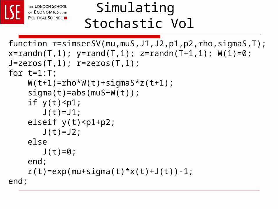
Simulating Stochastic Vol
function r=simsecSV(mu,muS,J1,J2,p1,p2,rho,sigmaS,T);x=randn(T,1); y=rand(T,1); z=randn(T+1,1); W(1)=0;J=zeros(T,1); r=zeros(T,1);for t=1:T; W(t+1)=rho*W(t)+sigmaS*z(t+1); sigma(t)=abs(muS+W(t)); if y(t)<p1; J(t)=J1; elseif y(t)<p1+p2; J(t)=J2; else J(t)=0; end; r(t)=exp(mu+sigma(t)*x(t)+J(t))-1;end;

Moving Averageof Simulated
sigmaS=.0025; rho=.96;r=simsecSV(mu,sigma,J1,J2,p1,p2,rho,sigmaS,T);T1=floor(T/7); masim=zeros(T1,2);for i=1:T1; in=(i-1)*7+1:(i-1)*7+7; masim(i,1)=std(r(in,1)); masim(i,2)=mean(r(in,1).^2); for j=1:7; t=(i-1)*7+j; masim(i,2)=masim(i,2)+(r(t,1)^2)/7; end;end;

>>X=[ones(T1-1,1) masim(1:T1-1,1)]; Y=masim(2:T1,1);>>[regcoef sterr a3 a4 rsq]=regress(Y,X);>>disp([regcoef sterr]); disp(rsq(1));>>subplot(2,1,1); plot(ma(:,1))>>subplot(2,1,2); plot(masim(:,1));

OptionalHomework (2)
Use the function from Homework (1) to simulate Microsoft daily returns for a period of a year many times, over and over again
Each time record the total return for the year This is called Monte-Carlo simulation How likely is it that Microsoft loses 30% in one year? How
likely is it to lose 40%? Separate the worst 5% of years from the next 95%. What is
the value lost at the 5% break? This is called Value at Risk, it is a commonly used risk measure
How sensitive is Value at Risk to jump parameters? Jump events are quite rare, do you think they are easy to estimate?

OptionalHomework (3)
Extend the model by adding stochastic volatility, try both the discrete Markov and the AR(1) process (AR(1) case done in class in file simsecSV.m)
How does this change kurtosis and likelyhood of tail events?
Plot a time series of squared Microsoft returns and squared simulated returns (with and without stochastic volatility)
Does it look like high times are followed by high times in the data? In the model with no stochastic vol? In the model with stochastic vol?
Do you see any problems with the AR(1) formulation for volatility?
Does Value at Risk change during high volatility and low volatility times?